how to use security analysis to improve portfolio...

How to Use Security Analysis to Improve Portfolio SelectionAuthor(s): Jack L. Treynor and Fischer BlackReviewed work(s):Source: The Journal of Business, Vol. 46, No. 1 (Jan., 1973), pp. 66-86Published by: The University of Chicago PressStable URL: http://www.jstor.org/stable/2351280 .

Accessed: 17/01/2013 08:44

Your use of the JSTOR archive indicates your acceptance of the Terms & Conditions of Use, available at .http://www.jstor.org/page/info/about/policies/terms.jsp

.JSTOR is a not-for-profit service that helps scholars, researchers, and students discover, use, and build upon a wide range ofcontent in a trusted digital archive. We use information technology and tools to increase productivity and facilitate new formsof scholarship. For more information about JSTOR, please contact [email protected].

.

The University of Chicago Press is collaborating with JSTOR to digitize, preserve and extend access to TheJournal of Business.

http://www.jstor.org

This content downloaded on Thu, 17 Jan 2013 08:44:23 AMAll use subject to JSTOR Terms and Conditions

http://www.jstor.org/action/showPublisher?publisherCode=ucpress

http://www.jstor.org/stable/2351280?origin=JSTOR-pdf

http://www.jstor.org/page/info/about/policies/terms.jsp


Jack L. Treynor and Fischer Black"

How to Use Security Analysis to Improve Portfolio Selection

It has been argued convincingly in a series of papers on the Capital Asset Pricing Model that, in the absence of insight generating expectations different from the market consensus, the investor should hold a replica of the market portfolio.' A number of empirical papers have demonstrated that portfolios of more than 50-100 randomly selected securities tend to correlate very highly with the market portfolio, so that, as a practical matter, replicas are relatively easy to obtain. If the investor has no special insights, therefore, he has no need of the elaborate balancing algorithms of Markowitz and Sharpe.2 On the other hand if he has special insights, he will get little, if any, help from the portfolio-balancing literature on how to translate these insights into the expected returns, variances, and covariances the algorithms require as inputs.

What was needed, it seemed to us, was exploration of the link between conventional subjective, judgmental, work of the security analyst, on one hand-rough cut and not very quantitative-and the essentially objective, statistical approach to portfolio selection of Markowitz and his successors, on the other.

The void between these two bodies of ideas was made manifest by our inability to answer to our own satisfaction the following kinds of questions: Where practical is it desirable to so balance a portfolio between long positions in securities considered underpriced and short positions in securities considered overpriced that market risk is completely eliminated (i.e., hedged)? Or should one strive to diversify a portfolio so completely that only market risk remains? As this implies, in the highly diversified portfolio market sensitivity in individual securities seems to contribute directly to market sensitivity in the overall portfolio, whereas other sources of return variability in individual securities seem to average out. Does this mean that the latter sources

* Editor, Financial A nalysts Journal; professor of finance, University of Chicago; and executive director, Center for Research in Security Prices.

1. William F. Sharpe, "Capital Asset Prices: A Theory of Market Equi- librium under Conditions of Risk," Journal of Finance 19, no. 3 (September 1964): 425-42; John Lintner, "The Valuation of Risk Assets and the Selection of Risky Investments in Stock Portfolios and Capital Budgets," Review of Economics and Statistics 57, no. 1 (February 1954): 13-37; and Jack L. Treynor's paper, "Toward a Theory of the Market Values of Risky Assets" (unpublished, 1961).

2. Harry Markowitz, Portfolio Selection: Efficient Diversification of In- vestments (New York: John Wiley & Sons, 1959; New Haven, Conn.: Yale Uni- versity Press, 1970); and William Sharpe, "A Simplified Model for Portfolio Analysis," Management Science 9 (January 1963): 277-93.

66



67 Security Analysis to Improve Portfolio

of variability are unimportant in portfolio selection? When balancing risk against expected return in selection of individual securities, what risk and what return are relevant? Will increasing the number of securities analyzed improve the diversification of the optimal portfolio? Is any measure of the contribution of security analysis to portfolio performance invariant with respect to both levering and turnover? How do analysts' opinions enter in security selection? Is there any simple way to characterize the quality of security analysis that will tell us when one analyst can be expected to make a greater contribution to a portfolio than another? What role, if any, does confidence in an analyst's forecasts have in portfolio selection? This paper offers answers to these questions.

The paper has a normative flavor. We offer no apologies for this. In some cases, institutional practice and, in some cases, law are short- sighted; in all cases they reflect what is by anybody's standard an old- fashioned idea of what the investment management business is all about. If we tried to develop a body of theory which reflected some of the constraints imposed institutionally and legally, it would inevitably be a theory with a very short life expectancy. Our model is based on an idealized world in which there are no restrictions on borrowing, or on selling securities short; in which the interest rate on loans is equal to the interest rate on short-term assets such as savings accounts; and in which there are no taxes. We expect that the major conclusions derived from the model will largely be valid, however, even with the constraints and frictions of the real world. Those that are not valid can usually be modified to fit the constraints that actually exist.

Certain recent research has suggested that professional investment managers really have not been very successful,' but we make the assumption that security analysis, properly used, can improve portfolio performance. This paper is directed toward finding a way to make the best possible use of the information provided by security analysts.

The basic fact from which we build is one that a number of writers have recognized-namely, that there is a high degree of comovement among security prices. Perhaps the simplest model of covari- ability among securities is Sharpe's Diagonal Model. As Sharpe sees it, "The major characteristic of the Diagonal Model is the assumption that the returns of various securities are related only through common relationships with some basic underlying factor. . . . This model has two virtues: it is one of the simplest which can be constructed without assuming away the existence of interrelationships among securities and there is considerable evidence that it can capture a large part of such interrelationships."4 This paper takes Sharpe's Diagonal Model as its

3. Michael Jensen, "The Performance of Mutual Funds in the Period 1945- 1964," Journal of Finiance 23 (May 1968): 389-416.

4. See Sharpe, n. 2.



68 The Journal of Business

starting point; we accept without change the form of the Diagonal Model and most of Sharpe's assumptions.

Use of the Diagonal Model for portfolio selection implies de- parture from equilibrium in the sense of all investors having the same information (and appraising it similarly)-as, for example, is assumed in some versions of the Capital Asset Pricing Model. The viewpoint in this paper is that of an individual investor who is attempting to trade profitably on the difference between his expectations and those of a monolithic market so large in relation to his own trading that market prices are unaffected by it. Throughout, we ignore the costs of buying and selling. This makes it possible for us to treat the portfolio-selection problem as a single-period problem (implicitly assuming a one-period utility function as given), in the tradition of Markowitz, Sharpe, et al. We believe that these costs are often substantial and, if incorporated into this analysis, would modify certain of our results substantially.

D E F I N I T I O N S

Following Lintner, we define the excess return on a security for a given time interval as the actual return on the security less the interest paid on short-term risk-free assets over that interval.

A regression of the excess return on a security against the market's excess return gives two regression factors. The first is the market sensitivity, or "beta," of the security; and, except for sample error, the second should be zero. We define the explained return on the security over a given time interval to be its market sensitivity times the market's excess return over the interval.

We define the independent return to be the excess return minus the explained return. The independent return, because of the properties of regression, is statistically independent of the market's excess return. Our model assumes that the "independent" returns of different securities are almost, but not quite, statistically independent. The "risk premium" on the ith security is equal to the security's market sensitivity times the market's expected excess return. Symbols for these concepts are defined as:

r riskless rate of return,

xi return on the ith security,

y- excess return on the ith security,

Ym excess return on the market,

bi market sensitivity of the ith security,

biym explained, or systematic, return on ith security,

zi independent return on ith security.

Let E [ ] and var [ ] represent the expectation and variance, respectively, of the variable in brackets. Then define



69 Security A nalysis to Improve Portfolio

Zi E[zi],

Y1n E[ym1].

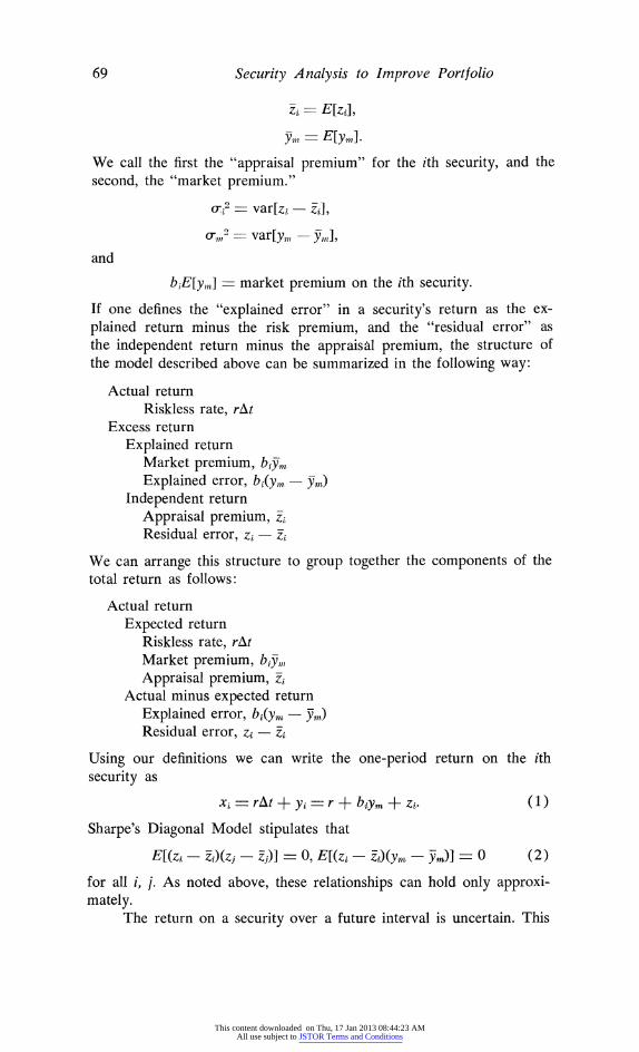
We call the first the "appraisal premium" for the ith security, and the second, the "market premium."

r7q,= var[zi -Zi,

02,2 var[yM -yell]

and

biE[y,,,] - market premium on the ith security.

If one defines the "explained error" in a security's return as the explained return minus the risk premium, and the "residual error" as the independent return minus the appraisal premium, the structure of the model described above can be summarized in the following way:

Actual return Riskless rate, rAt

Excess return Explained return

Market premium, b-y1,1 Explained error, bi(yn, -Y)

Independent return Appraisal premium, z- Residual error, zI -Z

We can arrange this structure to group together the components of the total return as follows:

Actual return Expected return

Riskless rate, rAt Market premium, by-1, Appraisal premium, Z-;

Actual minus expected return Explained error, bj(y,, - Yi) Residual error, Zi -Z

Using our definitions we can write the one-period return on the ith security as

xi rAt + yi r + biym +zi. (+1 )

Sharpe's Diagonal Model stipulates that

E[(zj - -)(zj - j)]- 0, E[(zj - )(ynL - 0 (2)

for all i, j. As noted above, these relationships can hold only approximately.

The return on a security over a future interval is uncertain. This




paper shares with Markowitz the mean-variance approach, implying normal return distributions. There is fairly conclusive evidence that the distribution is not normal, but that its behavior is similar to that of a normal distribution, so the model assumes a normal distribution as an approximation to the actual distribution. The qualitative results of the model should not be affected by this approximation, but the quantitative results should be modified somewhat to reflect the actual distribution.

However one defines "risk" in terms of the probability distribution of portfolio return, the distribution, being approximately normal, is virtually determined by its mean and variance. But under the assumptions noted here (finite variances and independence) the mean and variance of portfolio return depend only on the means and variances of independent returns for specific securities and on the explained return (and, of course, on the portfolio weights). On the other hand, risk in the specific security is significant to the investor only as it affects portfolio risk. Hence it is tempting to identify risk in the ith security with the elements in the security that contribute to portfolio variance-the variance of the independent return 0,2 ("specific risk") and the variance of explained return b 2 a .2 ("market risk"). In what follows, we will occasionally yield to this temptation.

Let the fraction of the investor's capital devoted to the ith security be hi. Using symbols defined above, the one-period return on his portfolio is

n n

Zhixi- rAt (Zhi h 1

n n

Z hi (yi + rAt) - rAt (Z h1 ) (3)

n

rAt +- L h-jyj. i=l

We note that, although there are three sources of return on the individual security-the riskless return, the explained return, and the independent return-only two of these are at stake in portfolio selection. Hence- forth we shall ignore the first term in equation (3).

Understanding the way in which portfolio mean and variance are influenced by selection decisions requires expansion of security return into all its elements. Excess return on the portfolio, expressed in terms of the individual securities held, is

n n

hibiym, + hizi. (4)

Evidently we have only n degrees of freedom-the portfolio weights




hi, with i - 1, . . ., n-in selecting among n + 1 sources of return. Since the market asset can always be freely bought or sold to acquire an explicit position hmn in the market asset, when we take this into account we have for the excess portfolio return the expression

?b n

(hm + Z hibi) ym + hizi. (5) i=1 i=1

It is obvious that availability of the market asset makes it possible to achieve any desired exposure to market risk, approximately inde- pendently of any decisions regarding desired exposure to independent returns on individual securities. In effect, we then have n + 1 mutually independent securities, where

n

hnw + I hm, + Adhibi, /ui =E(z+), i =1,.., n, /Jn+l =E[ym] (6) i=1

If we apply these conventions and run our summations from 1 to n + 1, we have for the mean and variance of the portfolio return, respectively,

n+1 n+1

fJ p hui p2 >ii: h2,O2. (7)

We take as our objective minimizing GP2 while holding [p fixed. We form the Lagrangian

n+1 n+1 2?2

Zh 2 A (8) i~~~l ~i=l

introducing the undetermined multiplier A, differentiate with respect to hi, and set the result equal to zero:

2hi 0-,2 -2 Xui ?. (9)

Solving for hi we have

hi A/Ot2 (10)

Substituting this result in equation (7) we have

n+1 n+1

/up A E J i72/0i2,0rp2= X2

E {i 2/c-4j2.(1 i==1 i=1

We see from (11) that the value of the multiplier X is given by

X = -2/Jp. (12)

The optimum position hi in the ith security (i 1, . . ., n) is given by equation (13):

hi = _. i = 1, . . ., n. (13) Up (r*




In order to obtain an expression for the optimal position hm in the market portfolio, we recall that

Uj.n+? E[ym] =lun

0r2 n+l varyy] = -l

and substitute these expressions together with the definitions of hl+ from equation (5) in (11) to obtain

n

Z hfbi + hm (14) i= 1

Multiplying both members of (10) by bi and summing we have

-hjb.; - E b1j/o-12, (15)

which can be substituted in (14) to give

hill A Z F/cX~) (16)

It was apparent in equation (5) that market risk enters the portfolio both in the form of an explicit investment in the market portfolio and implicitly in the selection of individual securities, the returns from which covary with the market. Equation (13) says "take positions in securities 1, . , n purely on the basis of expected independent return and variance." The resulting exposure to market risk is disregarded.

Equation (16) provides us with an expression for the optimal investment in an explicit market portfolio. This investment is designed to complement the market position accumulated in the course of taking positions in individual securities solely with regard to their independent returns. Under the assumptions of the Diagonal Model, position in the market follows the same rule as position in individual securities; but because market position is accumulated as a by-product of positions in individual securities, explicit investment in the market as a whole is limited to making up the difference between the optimal market position and the by-product accumulation (which may, of course, be negative, requiring an explicit position in the market that is short, rather than long).

Equation (16) suggests that the optimal portfolio can usefully be thought of as two portfolios: (1) a portfolio assembled purely with regard for the means and variances of independent returns of specific securities and possessing an aggregate exposure to market risk quite incidental to this regard; and (2) an approximation to the market portfolio. Positions in the first portfolio are zero when appraisal premiums are zero. Since the special information on which expected independent returns are based typically propagates rapidly, becoming fully dis-




counted by the market and eliminating the justification for positions based on this information, the first portfolio will tend to experience a significant amount of trading. Accordingly, we call it the "active portfolio."

It is clear from equation (10) that changes in the investor's attitude' toward risk bearing (X), or in his market expectations (do),

or in the degree of market risk (-m,2)-which, as we shall see, depends on how well he can forecast the market-have no effect on the proportions of the active portfolio.

The Capital Asset Pricing Model suggests that any premium for risk bearing will be associated with market, rather than specific risk. If investors in the aggregate are risk averse, then an investment in the market asset-explicit or implicit-offers a premium. We call this particular source of market premium "risk premium"-as opposed to "market premium" deriving from the investor's attempts to forecast fluctuations in the general market level. When all the appraisal premiums are zero, the optimal portfolio is therefore the market portfolio -even if the investor has no power to forecast the market. We shall call a portfolio devoid of specific risk "perfectly diversified." In other words, in our usage "perfect diversification" does not mean the absence of risk, nor does it mean an optimally balanced portfolio, except in the case of zero appraisal premiums.

In general, a given security may play two different roles simultaneously: (1) A temporary position based entirely on expected independent return (appraisal premium) and appraisal risk. As price fluctuates and the investor's information changes, the optimum position changes. (2) A position resulting purely from the fact that the security in question constitutes part of the market portfolio. The latter position changes as market expectations change but is virtually independent of expectations regarding independent return on the security. Hence we call the approximation to the market portfolio employed to achieve the desired level of systematic risk the "passive portfolio." The literal interpretation of equation (16) is that a desired explicit market position hMrb would be achieved by adding positions in individual securities in the proportions in which they are represented in the market as a whole. For example, let the fraction of the market as a whole comprised by the ith security be h?,. Then an explicit market position h.n can be achieved by taking positions h,,h ,, in the individual securities. These positions are, of course, in addition to positions taken with regard to specific return. Overall positions are then given by combining positions desired for fulfilling the two functions of bearing appraisal and market risk:

n

hi A -h miZ)nl J12 blL,/Oi2) + /UTi,-2 (17)

This is the result one would get by solving the Markowitz formula-




tion, under the assumptions of the Diagonal Model, in the absence of constraints. But it is not a solution of much practical interest, because approximations to the market portfolio add very little additional specific risk while being vastly cheaper to acquire than an exact pro rata replica of the market.

A practical interpretation of equation (16) is that portfolio selection can be thought of as a three-stage process, in which the first stage is selection of an active portfolio to maximize the appraisal ratio, the second is blending the active portfolio with a suitable replica of the market portfolio to maximize the Sharpe ratio, and the third entails scaling positions in the combined portfolio up or down through lending or borrowing while preserving their proportions. Because the investor's attitude toward risk bearing comes into play at the third stage, and only at the third stage, a second-stage definition of "goodness" that dis- regards differences in attitude toward risk bearing from one investor to another is possible.5

THE SHARPE AND APPRAISAL R A T I O S

From equation (10) we have, for the optimal holdings, hi - X/(r/, where, for the optimal second-stage portfolio, we have

n+1

Iu A, - 2/ Oi2

n+1 (18)

O-p2 - X2 E ki2/'i 2.

i=

How good is the resulting portfolio? A relationship between expected excess return and variance of return is obtained by forming

n+1

2 AX2 ( -i 2/i2) E (19)

X2 n+1

X2 ZzH2/ O.2 *= 1

The resulting ratio is essentially the square of a measure of goodness proposed by William Sharpe;6 we shall call it the Sharpe ratio. It is obviously independent of scale. The right hand expression readily partitions into two terms, one of which depends only on market forecasting and the other of which depends only on forecasting independent returns for specific securities:

5. See, for example, William Sharpe, "Mutual Fund Performance," Journal of Business 39 (January 1966): 119-38. %

6. Ibid.




%2n+I /02? 1 + Z /C<2/Oi2 0,P2 ~~~~~i=1

It is easily shown by writing out the numerator and denominator, and then simplifying as in equation (19), that the second term of (19) is the ratio of appraisal premium, squared, to appraisal variance. This number is obviously invariant with respect to changes in the holdings in the active portfolio by a scale factor, hence of shifts in emphasis between the active and passive portfolios. It measures how far one has to depart from perfect diversification to obtain a given level of expected independent return. Because it summarizes the potential contribution of security appraisal to the portfolio, we call it the appraisal ratio.

Consider, for example, two portfolio managers with the same information about specific securities and the same skill in balancing exposure to specific returns. One can generate a larger appraisal premium than the other simply by taking large positions in specific securities (relative to the market). Hence appraisal premium (as, for example, measured by the Jensen performance measure)7 is not invariant with respect to such arbitrary changes in portfolio balance. The fact that the appraisal ratio is invariant with respect to such changes commends it as a measure of a portfolio manager's skill in gathering and using information specific to individual securities. If, in addition to the same information specific to individual securities, two portfolio managers have the same market expectations, then their scale of exposure to specific returns (relative to their market exposure) should, of course, also be the same, as implied by equation (16). But in performance measurement, it is not safe to assume that the optimal balance will be struck by every portfolio manager. (How well he adheres to the optimal balance between market and specific risk is certainly one aspect of performance. But it is an aspect quite distinct from how well he uses security analysis.)

The appraisal ratio has much to recommend it as a measure of potential fund performance, although it does not directly measure the utility of the overall portfolio to investors. If "aggressiveness" refers to the amount of market risk borne by a diversified fund, and "activity" refers to the amount of trading undertaken in optimizing the active portfolio, then the second stage (at which the active portfolio is balanced against the passive portfolio) determines the degree of activity in the risky portion of the fund, and the third stage (at which the active portion is mixed or levered to obtain the balance between expected return and risk which meets the investor's personal objectives) determines the aggressiveness of the overall fund.

What happens to the degree of portfolio diversification as (1 ) the number of securities considered is increased? (2) the number of securities considered is kept constant while the contribution to the appraisal

7. See n. 3.




ratio of the average security is increased? Does the former improve the degree of diversification while the latter degrades it? We demonstrate below that the degree of diversification in an optimally balanced portfolio depends on these factors only as they influence the appraisal ratio. (It also depends on market ratio, but the latter is obviously independent of both the contribution to the appraisal ratio of the average security and the number of securities considered.) We also demonstrate that the higher the appraisal ratio (for a given market ratio) the less well diversified the resulting portfolio will be. In short, the more attractive incurring specific risk is relative to incurring market risk, the less well diversified an optimally balanced portfolio will be. Indeed, it is easily shown that at optimal balance we have

appraisal premium appraisal variance appraisal ratio ,(20)

market premium market variance market ratio

where market ratio is defined, analogously with appraisal ratio, as

(market premium)2 (21) market ratio - . (21)_____

market variance

The demonstration below actually applies to optimal (relative) holdings of any two assets whose specific returns are statistically independent. In particular, the "assets" consisting of the market, on one hand, and a weighted combination of independent returns, on the other, are statistically independent for any set of weights, including the optimal set. On the one hand, we have the contribution to the optimally balanced portfolio of market return, yen, with expectation } and variance 0m2.

On the other hand, we have the contribution from optimally balanced returns z, . . ., Zn,

with expectation Ala, defined by n

Hka Z h/ly, i= 1

and variance a-,2 defined by n

a2 2

h2Xr2 -' hi o'2.

i=l

This contribution is, of course, the essential part of the active portfolio, since the contribution of market risk to the overall portfolio is independent of the market risk in the active portfolio (see eq. [16]). It is also statistically independent of the market portfolio, since we have

n i

or y1 t hii hi ENzarms. 0.




Let optimal holdings for the market and active portfolios, respectively, be represented by h~, and ha. Then from equation (10) we have

ha _/-a/O0.1

ha~a Fa 2/0,a 2 (22)

hinFuln ,UI, 2/u-n2

which demonstrates the equality between the first and third fractions in (20). Squaring and then multiplying both sides by (tn)2/0('2) / (-Ca 2/Oa )

we have

ha2 0-a 2

/Ua2/0fa2 (23)

hilt2(m 2 ini2/0m2 (23)

which demonstrates the equality between the second and third fractions of (20). In an optimally balanced portfolio, total portfolio variance is given by

i = (} i= O (rt~~~~1ki 2 2y .o2 Z2 / )(

2 2

i=O 002 7T 2

1=1 0i2

where the first term is the contribution of market variance and the second is the contribution of the combined variance of the independent returns (i.e., the unique variance). Partitioning total variance into these two terms enables us to write the coefficient of determination pP2 expressing the fraction of total variance accounted for by systematic, or market, effect as

O2 pp

2 ~ ~ X PP ~~~~~~n

A0o2 1+ o2

n

1E i2 + 2

1-ko~~~~

_ 1 ~~~~(25) 1 appraisal ratio

m1 markett ratio




In this form it is clear that any improvement in the quality of security analysis, or in the number of securities analyzed at a given level of quality, can only cause an optimally balanced portfolio to become less well diversified.

Consider again the expression for appraisal ratio

n

appraisal ratio 2 (26)

On the average, half the securities analyzed will be overpriced and half

underpriced. Thus if short selling is permitted, on the average half the positions in an ideal active portfolio will be long positions and half short. Since the degree of market risk will generally be distributed among securities randomly with respect to the sign of the current price discrepancy, hence the sign of positions in the active portfolio,8 the expected level of market risk in an ideal active portfolio is zero. In the ideal case, therefore, the second-stage blending between active and passive portfolios is particularly simple: All the appraisal risk is in the active portfolio, and all the market risk is in the passive portfolio. When short selling is not permitted, however, the expected level of market risk in the active portfolio is the average level for the universe from which active securities are selected.- Half the terms in (26) are suppressed, thus on average reducing the appraisal ratio by half.

DERIVING FORECASTS OF

INDEPENDENT RETURNS FROM

SECURITY ANALYSIS

How are the appraisal premiums and variances for individual securities generated by the security analysis process? There are doubtless many ways of answering this question. The one that follows, which assumes a bivariate normal for the joint distribution of the analyst's opinion and the subsequent independent return, is certainly one of the simplest.

Presumably the analyst begins by appraising the security in question. We have shown that the composition of the active portfolio should be independent of expectations regarding the level of the market as a whole. It follows that, in order to be useful in selection of the active portfolio, the analyst's findings should be expressed in such a way that they are invariant with respect to his overall market expectations. Per- haps the easiest way for the analyst to generate opinions with the desired invariance property (under the independence assumptions of the Diagonal Model) is to estimate the value of the security (i.e., what the equilibrium price would be if all investors had his information) consistent with the consensus macroeconomic forecast implicit in the general level of security prices obtaining at the time of the estimate. The value an analyst

8. See eq. (27).



79 Security A nalysis to Improve Portfolio

assigns to a security may be either greater or less than its present price. (Some analysts may be unwilling to assign a value to the security; they may be more comfortable giving a "buy" price and "sell" price, and we can take the point halfway between as their estimated value.)

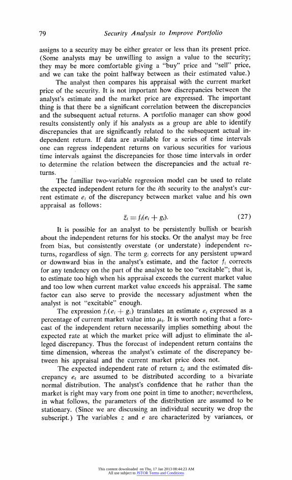
The analyst then compares his appraisal with the current market price of the security. It is not important how discrepancies between the analyst's estimate and the market price are expressed. The important thing is that there be a significant correlation between the discrepancies and the subsequent actual returns. A portfolio manager can show good results consistently only if his analysts as a group are able to identify discrepancies that are significantly related to the subsequent actual independent return. If data are available for a series of time intervals one can regress independent returns on various securities for various time intervals against the discrepancies for those time intervals in order to determine the relation between the discrepancies and the actual returns.

The familiar two-variable regression model can be used to relate the expected independent return for the ith security to the analyst's current estimate ei of the discrepancy between market value and his own appraisal as follows:

%i - fi(e1 + gO). (27)

It is possible for an analyst to be persistently bullish or bearish about the independent returns for his stocks. Or the analyst may be free from bias, but consistently overstate (or understate) independent returns, regardless of sign. The term gi corrects for any persistent upward or downward bias in the analyst's estimate, and the factor fi corrects for any tendency on the part of the analyst to be too "excitable"; that is, to estimate too high when his appraisal exceeds the current market value and too low when current market value exceeds his appraisal. The same factor can also serve to provide the necessary adjustment when the analyst is not "excitable" enough.

The expression fi(ei + gi) translates an estimate ei expressed as a percentage of current market value into ,ui. It is worth noting that a forecast of the independent return necessarily implies something about the expected rate at which the market price will adjust to eliminate the al- leged discrepancy. Thus the forecast of independent return contains the time dimension, whereas the analyst's estimate of the discrepancy between his appraisal and the current market price does not.

The expected independent rate of return zi and the estimated discrepancy e.i are assumed to be distributed according to a bivariate normal distribution. The analyst's confidence that he rather than the market is right may vary from one point in time to another; nevertheless, in what follows, the parameters of the distribution are assumed to be stationary. (Since we are discussing an individual security we drop the subscript.) The variables z and e are characterized by variances, or




their respective square roots s_ and s,. A third parameter is necessary to complete the specification of this distribution, namely the correlation coefficient p between the variables z and e. In composing the active portfolio we are interested in the conditional distribution of z given e, or zle. Unless an analyst is able to anticipate all the events affecting the price, hence the return, on a security, some portion of the independent return variance remains unexplained by his forecasts.

In terms of the parameters characterizing the joint normal distribution of e and z, equation (27) can be rewritten

z p(i-) (e+g). (28)

Regressing z against e, we get estimates of the slope coefficient p(S,/S,) and the constant term p(SI/S,)g. It is important to look at the signi- ficance of the regression factors found. Normally data covering a number of intervals will be needed to show that any of the regression factors is significantly different from zero. Some of the deviations of the regression coefficients from zero will be due to sample error rather than an actual relation between analysts' estimates and independent returns.

We are also interested in the residual variance (i.e., that part of the total variance in the independent returns on a security not explained by the analyst's estimate). The amount of a security that should be held in the active portfolio depends not only on the independent return expected on the security but also on the residual variance of the independent return around its expected value. The variance -o2 of forecast errors between z and actual z is

0,2 =var [zle] (1 - p2)SZ2. (29)

We saw in equation (26) that the value of the appraisal ratio for an optimally diversified portfolio depends only on the value of the ratio

z2/of22 for individual securities. Given the analyst's current appraisal

(e), the conditional value of this ratio is -222

z p (e + g)2 (30)

2 i-p2 se2

The right-hand factor in equation (30) is, of course, merely the square of the analyst's estimate, corrected for bias and normalized to unit variance. The current contribution of the security in question to the appraisal ratio of the active portfolio also depends on the analyst's ability to forecast fluctuations in independent return successfully (p).

To say that one analyst is "better" than another implies something about the expected value of the contributions of their respective securities to an active portfolio averaged over a series of holding periods

9. See, for example, Harald Cramer, The Elements of Probability Theory (Princeton, N.J.: Princeton University Press, 1946), pp. 141 and 142.




and without specific reference to the forecasts obtaining at the beginning of each holding period. At the beginning of each holding period, expectations of independent returns are formed as described above. We con- tinue to denote these expectations by a bar over the appropriate symbol: t. But now consider a longer-run expectation, based purely on the joint distribution of estimated and actual return, denoting the latter kind of expectations by E[ . . .]: We note that, since the expected value over time of (e + g) is zero (with g correcting for any bias in e), the expected value of (e + g)2 is given by

E[(e + g)2] - var[e] Se2. (31)

Thus if the expectation of equation (30) is taken with respect to the distribution of the analyst's forecasts, we have

E [] p2 (32)

In the absence of prior knowledge concerning the analyst's current forecast, therefore, the potential contribution of the security in question to the optimum active portfolio depends solely on p. The larger p is, the more the security contributes to the optimal active portfolio. The expression in equation (32) can be thought of as the ratio of the variance in residual price changes explained by the analyst's estimates to the variance left unexplained.

In any forecasting problem, there are three kinds of variables: (1) the dependent variable (in this case, independent return); (2) one or more independent explanatory variables (in this case, the analyst's opinion, etc.); and (3) the expected value, or maximum-likelihood forecast of the dependent variable, based on knowledge of the independent variables. In the case considered in this section, the explanatory variable was the difference between the analyst's estimate of value and current price.

When (e) is treated as the discrepancy between current price and appraised value, then, however long a discrepancy has been outstanding, the fraction expected to be resolved in the next holding period is the same (or, equivalently, the probability of complete resolution in the next period is the same). The fraction to be resolved (or the probability of resolution) is independent of the scale of the discrepancy. No allow- ance is made for the possibility that the rate of resolution may depend in part on the kind of insight leading to identification of the discrepancy or on the source of the insight.

For any or all these reasons, the portfolio manager may prefer to supply his own approach to formulating forecasts of independent return. If (e) is interpreted as representing the explanatory variable upon which the forecast is based-whether derived by fundamental, technical, or other means-the regression model in which (e) appears (eq. [27]) is reduced to the less ambitious role of relating the explanatory variable, forecast, and actual return, without linking the forecasting process di-




rectly to the determinations of the security analyst. The price of this decision is, of course, that the process by which the explanatory variable is generated then becomes a black box, determination of whose contents is outside the scope of the model presented here.

The fact that (e) is susceptible of the more general interpretation means, however, that the results regarding the role of the coefficient of determination p2 in portfolio selection are not limited to the model presented here, in which price discrepancy is itself the explanatory variable, but are in fact as general as the application to the forecasting problem of the regression model itself.

All the preceding comments on forecasting the independent return apply to forecasting the market return Yn.

S U M M A R Y

1. It is useful in balancing portfolios to distinguish between two sources of risk: market, or systematic risk on the one hand, and appraisal, or insurable risk on the other. In general it is not correct to assume that optimal balancing leads either to negligible levels of appraisal risk or to negligible levels of market risk.

2. Without any loss in generality, any portfolio can be thought of as having three parts: a riskless part, a highly diversified part (that is, virtually devoid of specific risk), and an active part which in general has in it both specific risk and market risk. The amount of market risk in the active portfolio is unimportant, so long as one has the option of increasing or reducing market risk via the passive portfolio. The overall portfolio can usually be improved by taking a long or short position in the market as a whole.

3. The rate at which a portfolio earns riskless interest is independent of how the portfolio is invested or whether or not the portfolio is levered and depends only on the current market value of the investor's equity.

4. The rate at which the portfolio earns risk premium depends only on the total amount of market risk undertaken and is independent of the size of the investor's equity and of the composition of his active portfolio.

5. Optimal selection in the active portfolio depends only on appraisal risk and appraisal premiums and not at all on market risk or market premium; nor on investor objectives as regards the relative im- portance to him of expected return versus risk; nor on the investment manager's expectations regarding the general market. Two managers with radically different expectations regarding the general market but the same specific information regarding individual securities will select active portfolios with the same relative proportions. (Here, as elsewhere in this paper, we ignore possible differences in the tax objective, liquidity considerations, etc.)

6. The appraisal ratio depends only on (a) the quality of security




analysis and (b) how efficiently the active portfolio is balanced. It is independent of the relative emphasis between active and passive portfolios and of the degree to which the risky portfolio is levered or mixed with debt. It is also independent of the market premium. Obviously, it is not necessary for a professionally managed fund to be optimal in terms of all three stages in order to be socially (or economically) successful: An individual investor may choose to perform the third-stage balancing himself, with the appropriate amount of personal borrowing or lending. He may even perform the second-stage balancing himself, determining the appropriate emphasis between a brokerage acount or ''go-go" fund on the one hand and a virtually passive old-line mutual fund or living trust on the other. On the other hand, any attempt to compare the skill with which professional investment managers select securities (i.e., performs the first-stage balancing) using historical rates of return must be designed invariant with respect to second- and third- stage balancing policies.

7. The security analyst's potential contribution to overall portfolio performance over time depends only on how well his forecasts of future independent returns correlate with actual independent returns, and not on the magnitude of these returns.

A P P E N D I X

In his paper, "Simplified Model for Portfolio Analysis,"'10 William Sharpe proposes the following model of the return from a risky security:

R- Ai, + BJ + C*

I = An+, + Cn+,1 (Al)

where A,,+, and the A, are constants, and C,,+1 and the Ci are random variables with expected values of zero and variances Qi and Q,,+1, respectively. Sharpe postulates that the covariances between C, and C1 are zero for all values of i and ] (i 7/ j).

As Sharpe sees it "the major characteristic of the Diagonal Model is the assumption that the returns of various securities are related only through common relationships with some basic underlying factor.... This model has two virtues: it is one of the simplest which can be constructed without assuming away the existence of interrelationships among securities and there is considerable evidence that it can capture a large part of such interrelationships."" Regarding the way the model is intended to be used, Sharpe says, "The Diagonal Model requires the following predictions from a security analyst: (1) the values of Ai, Bi, and Qi, for each of n securities, (2) values of A,+1 and Q,, 1 for the Index."'21 In order to give the best possible results, the analyst's estimates of the Ai should be free from bias, consistent from one security to the next, and reflect both the analyst's current appraisal of the

10. See Sharpe, n. 2. 1 1. Ibid. 12. Ibid.




securities and his knowledge of current market prices. It is, of course, also necessary that he have a rational basis for estimating the Q,. If there is indeed a significant degree of comovement among securities, then his estimates must recognize this fact.

In the equations which follow, r is the risk-free interest rate. Let E[ represent the expectation of the random variable in the brackets, var[ ] the variance, and cov[ , ] the covariance of the two variables within the brackets. If Sharpe's market index I(z A,,--1 + C,,+1) can be identified with the return on market as a whole, then, according to the Sharpe-Lintner- Treynor theory, expected return on the ith security in equilibrium must satisfy

E[Ri, r] =k cov [Ri, I]

k cov [As, + Bi(A i+I + C?1 ) + Ci,, A,+I + C ?+].

Eliminating constant terms and terms in Ci, which by definition have zero covariance with 1, we have

E[Ri] = Bik var Ca + - BikQ,, +?1

In equilibrium, therefore, we have

E[Ri] r + BikQ,, + 1 (A2)

On the other hand, the Sharpe Diagonal Model stipulates that

E[Ri - Ai + BiA,+1.

The only way both equations can hold for all values of B1 is if

A. - r

A~n+1 =~1 {1 (A3)

It is clear that, in a dynamic equilibrium in which all investors evaluate new information simultaneously, A is the riskless rate and A,, + B is the expected excess return on the ith security.

Once we abandon the assumption that all investors have the same information, it is no longer true that expected excess return on the ith security is proportional to B,. It is apparent that the values of Ai, i = 1, . . . , n, A,, 1

leading to a given set of expectations of the Ri are not uniquely determined by specifying expected returns for a set of securities. A set of values that implies that half the universe of securities are overpriced relative to the current market and half are underpriced, that is, the set for which

I Mi(Aj - r) O. 0,(A4) i

we call market neutral. In order to eliminate the ambiguity, we shall assume henceforth the Ai

are implicitly defined to be market neutral. Then Ai is the sum of the pure rate and expectation of a disequilibrium price movement, and A,,+1 is the expected excess return on the market. In the case in which an investor has special information on the ith security, Ai will differ from the equilibrium




value by an amount which we will call the appraisal premium, in deference to the source of the premium:

appraisal premium - Ai -i

A i appraisal premium + riskless rate. (A5)

We can now summarize our interpretations of the symbols in Sharpe's Diagonal Model (modified slightly as noted above):

1. Ai = the sum of the risk-free rate and the appraisal premium on the ith security.

2. A,,+1 = the investor's expectation of excess return for the market as a whole. If he is not trying to outguess the overall market, it is the premium offered to investors generally for bearing market, or systematic, risk.

3. Bi = the volatility of the ith security-that is, its degree of sensitivity to market fluctuations.

4. Cl+1 = the difference between actual return on the market and expected return on the market. Its variance is Q, +1. If an analyst has no power to forecast market fluctuations, Q,,+1 is the variance of the market return.

5. Ci = the difference between actual return on the ith security and the return explained by the actual market return (plus the prime interest rate). Its variance is 0i. If an analyst has no power to forecast the independent return, Qi is the residual variance of return of the ith security re- gressed against the market.

Now consider again Sharpe's expression for return on the ith security: Ri = A + Bi(A,,+1 + C, +1) + Ci. Can we define I = A, +1 + C,, + I in terms of the Ri? If not, then I is not truly an "index" in the sense of return on a market average. Let Mi be the total market value of the ith security. Then define

I A,, 1 + C, +1 + Mi(Ri- r). (A6)

When the so-called market index I is defined in this way, one of the assumptions in Sharpe's model no longer holds exactly. Forming the sums of each term in equation (A 1) over the whole set of securities, weighted by respective market values, and rearranging we have

E M,(Ri - A i) (A,, + 1 + C,, + 1) MjBi + E MiCi. (A7)

Substituting from equation (A6) and invoking equation (A4) we have

(A,,+ 1 + C,,+0 (IM - IMB) I MC.

This expression can hold in general only if

E Mici 0

l EMl (A8)

The second equation merely requires that the weights sum to 100 per-




cent. The first, however, is a constraint on the independence of the Ci. The constraint conflicts slightly with Sharpe's own model, which postulated E[C, Cj] = 0 for all i d& j, and E[CiC,, +] = 0 for all i. The conflict arises from a confusion-possibly unintended or possibly intended-in the Diag- onal Model between an underlying explanatory variable to which all securities are sensitive in greater or lesser degree, and a Market Index such as I M(R- r).



how to use security analysis to improve portfolio...

Documents