Errata

Title & Document Type:

Manual Part Number:

Revision Date:

HP References in this Manual This manual may contain references to HP or Hewlett-Packard. Please note that Hewlett-Packard's former test and measurement, semiconductor products and chemical analysis businesses are now part of Agilent Technologies. We have made no changes to this manual copy. The HP XXXX referred to in this document is now the Agilent XXXX. For example, model number HP8648A is now model number Agilent 8648A.

About this Manual We’ve added this manual to the Agilent website in an effort to help you support your product. This manual provides the best information we could find. It may be incomplete or contain dated information, and the scan quality may not be ideal. If we find a better copy in the future, we will add it to the Agilent website.

Support for Your Product Agilent no longer sells or supports this product. You will find any other available product information on the Agilent Test & Measurement website:

www.tm.agilent.com Search for the model number of this product, and the resulting product page will guide you to any available information. Our service centers may be able to perform calibration if no repair parts are needed, but no other support from Agilent is available.

I JitterAnalysisUsing theHP 54120Family of.DigitikingOscilloscopes

1

Introduction

Why Jitter isImportant

Types of Jitter

The histogram techniques of the HP 54120 series of digitizing oscil-loscopes allow comprehensive characterization of jitter. This productnote provides the procedures for measuring common types of jitteron an HP 54120 digitizing oscilloscope using histograms. To under-stand how the histogram techniques of an HP 54120 can be usedfor jitter measurements, types of jitter and their effects will bereviewed. Jitter measurement configurations are outlined and mea-surement results representing a cross section of 54120’s are given.

Jitter describes the random time uncertainty of a waveform eventrelative to a particular point. In digital hardware operation, data isplaced on the input of a device and “clocked” into that device with apulse edge. The device performs some operation with the data andprovides an output. Timing relationships between clock, input sig-nals, and output signals are all crucial to error-free data transfer.

The jitter between a clock and input data signal edges can causeerroneous transfers of data. Invalid data transfer becomes increas-ingly probable as the amount of jitter approaches the width of thetime window during which data can be successfully transferred.Particularly at high data rates, it is essential to minimize jitterbetween signals so that the clocking device can initiate error-freetransfer of information.

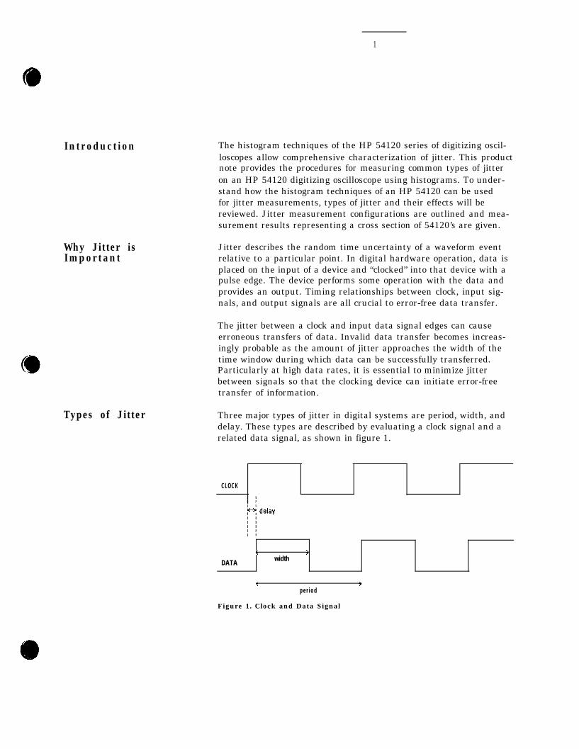
Three major types of jitter in digital systems are period, width, anddelay. These types are described by evaluating a clock signal and arelated data signal, as shown in figure 1.

CLOCK

< >DATA width

<p e r i o d

Figure 1. Clock and Data Signal

2

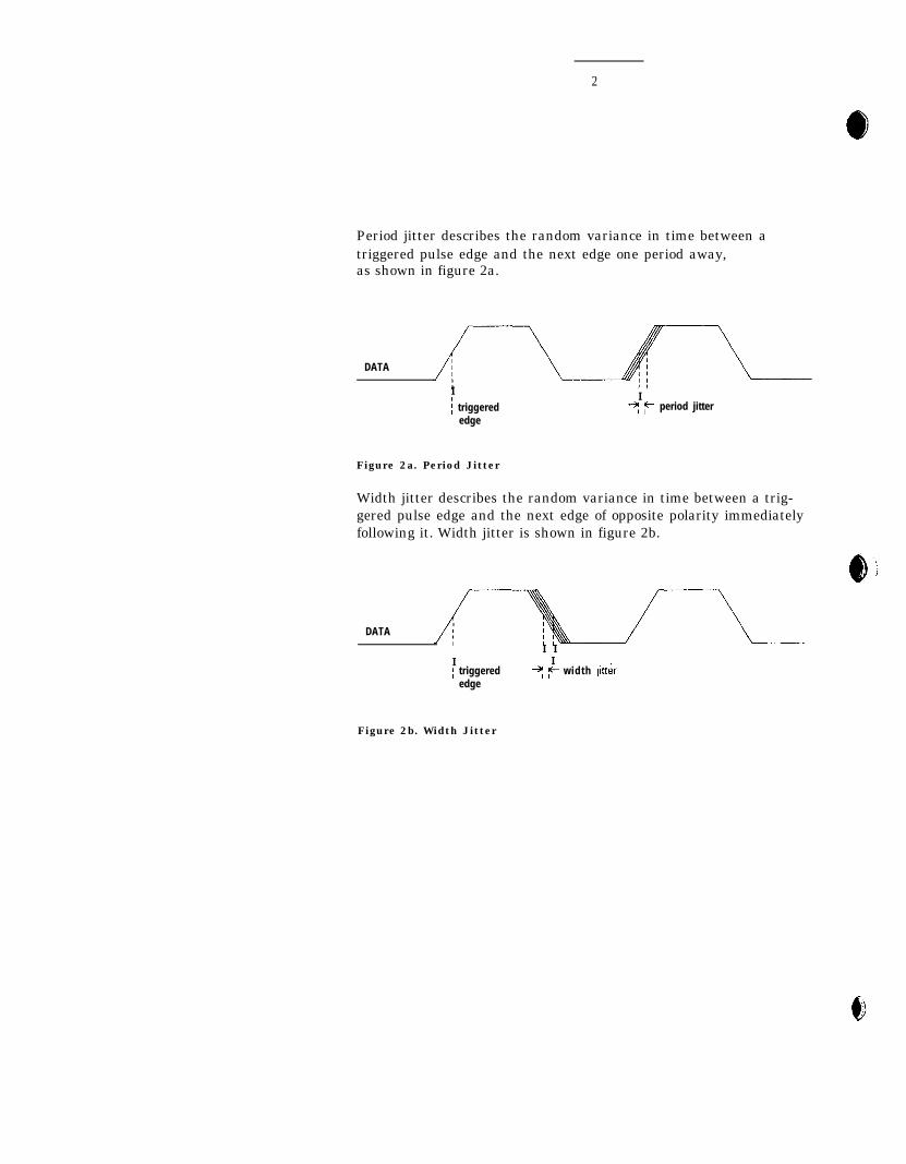
Period jitter describes the random variance in time between atriggered pulse edge and the next edge one period away,as shown in figure 2a.

DATA

Ii triggered) edge

I I7 7 period jitter

I I

Figure 2a. Period Jitter

Width jitter describes the random variance in time between a trig-gered pulse edge and the next edge of opposite polarity immediatelyfollowing it. Width jitter is shown in figure 2b.

DATA

I I III I I; triggered jl 7 width j&rI edge I I

Figure 2b. Width Jitter

3

AnalogOscilloscopeRepresentation

Delay jitter describes the random variance in time between a clockedge and an associated data edge, or between two data signals.Delay jitter is shown in figure 2c.

CLOCK

i triggeredt edge

DATA

--d k- delay jitterII

Figure 2c. Delay Jitter

Both analog and digitizing oscilloscopes provide direct viewing ofjitter on their screens.

With a standard analog oscilloscope, jitter is seen as a band of illu-minated phosphor, where the brightest section corresponds to thelocation where the edge occurs most often. A distribution of lowerintensities indicates where the edge has lower occurrence. Typically,the CRT intensity is increased until just before blooming occurs andthe limits of jitter are recorded as a peak-to-peak jitter measure-ment. A disadvantage in analog scopes is that the jitter measure-ment is dependent on the intensity setting, and the extremes of thejitter may not be sufficient to light the screen phosphor, yieldingsomething less than peak-to-peak jitter. Analog storage scopes over-come part of this problem by building up a trace of jitter and keep-ing it on the screen; however, storage scopes are especially suscepti-ble to blooming.

It follows that a digital oscilloscope can provide repeatable andquantifiable results, whereas an analog scope cannot.

4

DigitizingOscilloscopeRepresentationWith Histograms

An accurate approach to measuring jitter is to use histograms in adigitizing oscilloscope to perform a statistical analysis on a distri-bution of jitter. Standard deviation ( sigma or RMS 1 is the mostaccurate way to characterize jitter. For normal distributions, sigmaprovides insight to the distribution of the jitter and peak-to-peakdoes not. The value of peak-to-peak jitter is either six or eight timessigma depending on your definition of peak-to-peak jitter. Six timessigma equates to 99.74% of the area bounded by the peak-to-peakjitter from Gaussian noise.

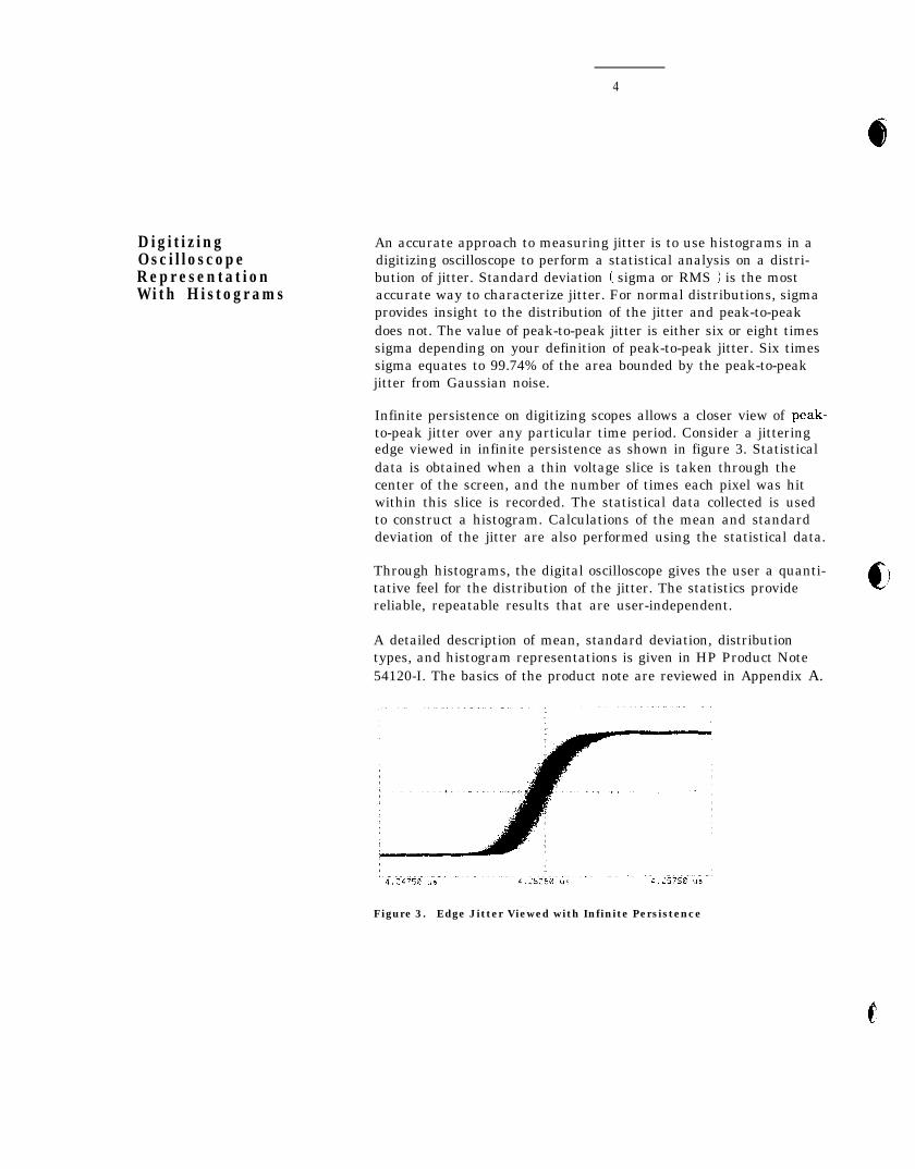
Infinite persistence on digitizing scopes allows a closer view of peak-to-peak jitter over any particular time period. Consider a jitteringedge viewed in infinite persistence as shown in figure 3. Statisticaldata is obtained when a thin voltage slice is taken through thecenter of the screen, and the number of times each pixel was hitwithin this slice is recorded. The statistical data collected is usedto construct a histogram. Calculations of the mean and standarddeviation of the jitter are also performed using the statistical data.

Through histograms, the digital oscilloscope gives the user a quanti-tative feel for the distribution of the jitter. The statistics providereliable, repeatable results that are user-independent.

A detailed description of mean, standard deviation, distributiontypes, and histogram representations is given in HP Product Note54120-I. The basics of the product note are reviewed in Appendix A.

Figure 3. Edge Jitter Viewed with Infinite Persistence

c

5

IdentifyingScope Jitter

/ slgnal

~ .-__--.

f

/’

-__ _ t h r e s h o l d

An additional component of jitter due to the oscilloscope itself isinherent in any jitter measurement. It is important to characterizescope jitter and separate it from the measurement so that only thesignal jitter remains. Two major sources of scope jitter are triggerthreshold and scope time base delay.

Trigger threshold jitter originates in the trigger circuit. A triggercircuit contains a comparator that looks for a slope polarity and alevel. All circuits produce some amount of thermal noise which isusually assumed to be Gaussian. When a signal crosses a compara-tor level, trigger threshold jitter is formed in the comparator outputfrom noise originating in the trigger circuitry. See figure 4 for a pic-torial description of the formation of jitter as a signal crosses athreshold. The faster the slew rate (AV/At), the less effect this noisehas on producing jitter.

signal with , ,J

signalwith nome

threshold

Idealno nofse

and no ptterLow slew rate High slew rate

high litter low jitter

Figure 4. The Formation of Jitter as a Signal Crosses a Threshold

Time base delay jitter originates in the course and fine pro-grammable delays of the time base. The coarse programmable delayis derived from counters driven by a 250 MHz oscillator. The 250MHz oscillator has a 0.1% frequency accuracy which introduces asmall amount of jitter. The fine programmable delay involves aramp voltage crossing a threshold. Any signal crossing a thresholdwill develop some amount of jitter. The amount of jitter is depen-dent on the amount of noise on the signal and the slope of the signalas it crosses the threshold.

6

HP 54120Specified Jitter

Oscilloscope jitter is specified to be within certain limits. Actualjitter is usually significantly less than this amount. Total scopejitter (including trigger threshold and time base delay jitter) isspecified in the following equation:

Jitter (RMS) < 5 ps + (5x10-a x scope delay setting)

For example, with a scope delay setting of 100 ns, the specifiedjitter is 5 ps + (5x10-5 x 100 ns) = 10 ps (RMS).

Hewlett-Packard guarantees performance to the extent of normalspecifications. Typically, HP 54120’s out-perform the jitter specifica-tions given in this document.

Basic Measurementsand ConfigurationsUsing a DigitizingOscilloscope

In the previous sections, the implications of period, width, delay,and scope induced jitter were discussed. In this section you will learnhow scope and signal jitter measurements are configured witha digitizing oscilloscope. Examples of measurements performed witha typical HP 54121T are provided to give a general idea of expectedresults.

Measurement ofHP 54120 Jitter

Measurement ofScope TriggerThreshold Jitter

Consider the following when making jitter measurements with anHP 54120:

HP 54120 Digitizing Oscilloscopes use a sequential sampling sys-tem whereby a single sample point is taken with each trigger.

There is a minimum delay of 16 ns between a trigger event and anactual acquisition. Therefore, a minimum delay line of 20 ns isrequired in the signal path to view the triggered edge at the centerof the screen. The delay line is important because scope induced jit-ter must be measured on the triggered edge so that it can later beremoved from the measured jitter of interest.

A number of measurements were performed to determine typicaltrigger threshold jitter and time base delay jitter. An HP 8341Bsweeper was selected as the signal source for frequency stabilityand spectral purity.

For this publication, trigger threshold jitter was measured for anumber of sinusoidal inputs. Measurements were performed bydividing the signals with a power splitter, triggering the scope withone output of the power splitter, and feeding the other outputthrough a delay line. The triggered edge then appeared on thescreen as close as possible to the minimum 16 ns delay. The testsetup is shown in figure 5. The triggered edge appeared at approx-imately 26 ns (22 ns delay line plus cabling at 1.2 ns/ft).

cj

7

Signal Generator Test Set Delav Line 122nsl,

Figure 5. Test Setup for Measuring Scope Trigger Threshold Jitter, SignalPeriod and Signal Width Jitter.

To properly characterize any scope, scope trigger threshold jittermeasurements must be made on the triggered edge of the signal tobe measured. To ensure that the triggered edge was correctly identi-fied, the source frequency was varied slightly while observing thewaveform. The triggered edge remained stationary while all otheredges moved. To view jitter, the waveform was expanded about thetriggered edge.

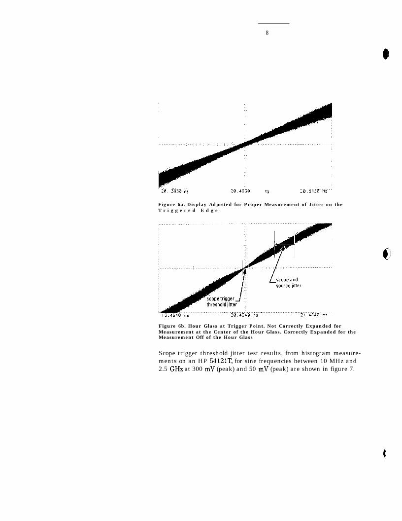
To obtain the most accurate jitter measurements, always increasetime base resolution and decrease channel display mVldiv settinguntil the jitter to be measured covers at least one division on thescreen. See figure 6a.

When the source has significant broadband noise, an hour glassshape appears at the exact trigger point. See figure 6b. When anhour glass ispresent, scope trigger threshold jitter is measured atthe center of the hour glass. Jitter measured on the triggered edgeoff of the hour glass is the combined jitter from the scope triggerthreshold jitter and the broadband noise of the signal being mea-sured. Signal noise jitter can be calculated by the followingequation:

___.--r/-M=dT 1 M e a s u r e d \z

8

20’. j830 ni 10.48:0 ns “5

Figure 6a. Display Adjusted for Proper Measurement of Jitter on theT r i g g e r e d E d g e

Figure 6b. Hour Glass at Trigger Point. Not Correctly Expanded forMeasurement at the Center of the Hour Glass. Correctly Expanded for theMeasurement Off of the Hour Glass

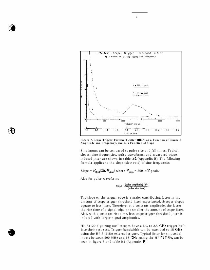
Scope trigger threshold jitter test results, from histogram measure-ments on an HP 5412113 for sine frequencies between 10 MHz and2.5 GHz at 300 mV (peak) and 50 mV (peak) are shown in figure 7.

9

I HP54120E Scope Trigger Threshold JitterAs a Function of Amplitude and Frequency

A - 300 mV peak

R = 50 mV peak__.-_

- - - -Or A : ++--t--c----- --t--c- : : : : : : --u--cI

0 50 0 1 0 0 0 1 5 0 0 2000 2 5 0 0

FREOUENCY IN MHz

k----co ,r-+-- -4;--.4~-. . -.-t;- .--- ;t,--.-.;t;--~...-~-~5

Slope in mV/ps

Figure 7. Scope Trigger Threshold Jitter (RMS) as a Function of SinusoidAmplitude and Frequency, and as a Function of Slope

Sine inputs can be compared to pulse rise and fall times. Typicalslopes, sine frequencies, pulse waveforms, and measured scopeinduced jitter are shown in table Bl (Appendix B). The followingformula applies to the slope (slew rate) of sine frequencies

Slope = (fm,,,)(2Tc V,,,) where V,,, = 300 mV peak.

Also for pulse waveforms

S,ope = (pulse amplitude) (0.8)-.(pulse rise time) -

The slope on the trigger edge is a major contributing factor in theamount of scope trigger threshold jitter experienced. Steeper slopesequate to less jitter. Therefore, at a constant amplitude, the fasterthe rise time of a signal edge, the smaller the amount of scope jitter.Also, with a constant rise time, less scope trigger threshold jitter isinduced with larger signal amplitudes.

HP 54120 digitizing oscilloscopes have a DC to 2.5 GHz trigger builtinto their test sets. Trigger bandwidth can be extended to 18 GHzusing the HP 54118A external trigger. Typical jitter for sinusoidalinputs between 500 MHz and 18 GHz, using the HP 54118A, can beseen in figure 8 and table B2 (Appendix B).

10

Q

Measurement ofScope Time BaseDelay Jitter

H P 5 4 1 2 0 6 S c o p e T r i g g e r T h r e s h o l d J i t t e rAs a Function of Amplitude and Frequency

A = 300 mV peak

B - 50 mV peak

0 *+- t----t -+---t--- ,-~--~-ti~-~-~~t-tt-t~------

0 500 1000 1500 2000 2500

FREQUENCY IN MHz

Figure 8. Typical Jitter (RMS) in High Bandwidth Triggering Using the HP5 4 1 1 8 A

Scope time base delay jitter can be of concern in any measurementwhere scope delay is used to bring an edge of interest on to thescreen.

Measurements of the time base delay jitter of a typical HP 54121Twere made using a 500 mV p-p, 500 MHz sine wave from anHP 8341B sweeper.

The trigger edge was brought to screen using a power splitter and adelay line as in figure 5. The amount of jitter was noted so thatscope induced jitter could be removed from the signal jitter mea-surement. Next, pieces of precision high-bandwidth cable wereinserted, one at a time, and scope delay was increased each time tobring the edge back on screen. Jitter results are shown in table 1.Removing scope jitter from measurements is discussed in a follow-ing section. The equation used for the corrected results in table 1 is

l Measurernentmade off of the hourglass If present

a

This data indicates that scope time base delay jitter is negligiblewithin the first 60 ns of scope delay.

11

Table 1. Scope Delay vs Jitter

Scope Measured RMS Corrected RMSDelay (ns) Jitter (ps) Delay Jitter (ps)22.58 1 . 0 N. A.26.09 1 . 1 0 . 4 629.78 1 . 1 0 . 4 633.46 1 . 1 0 . 4 637.14 1 . 1 0 . 4 640.88 1 . 1 0.4643.55 1 . 1 0.4646.20 1 . 1 0 . 4 649.68 1 . 1 0 . 4 653.37 1 . 1 0 . 4 657.06 1.2 0 . 6 660.74 1.3 0 . 8 3

Similar scope time base delay jitter results were obtained by observ-ing the highly stable output signal from an HP 8341B sweeper atvarious scope delay settings and noting the amount of scope timebase delay jitter. The signal used for the measurement was 500MHz, 500 mV p-p. Uncorrected and corrected test results are shownin figure 9. Minimum jitter of 0.9 ps RMS is only seen at the exacttrigger point. Measured jitter immediately increases to 3.0 ps oneither side of the trigger point due to broadband noise in the sweep-er. This noise is the cause of the hour glass appearance of the trig-gered edge. Delays over 500 ns were not considered, since the delayis restricted to 10s x screen diameters.

HP54120 TIMEBASE DELAY VS JITTERUsing a 500 MHz sinewave at 500mV p-p

SCOPE DELAY IN NS

Figure 9. Uncorrected Measured Scope Delay Jitter as a Function ofScope Delay

12

MeasurementConfiguration forPeriod and WidthJitter of a Signal

Measurement,Configuration forDelay Jitterof a Signal

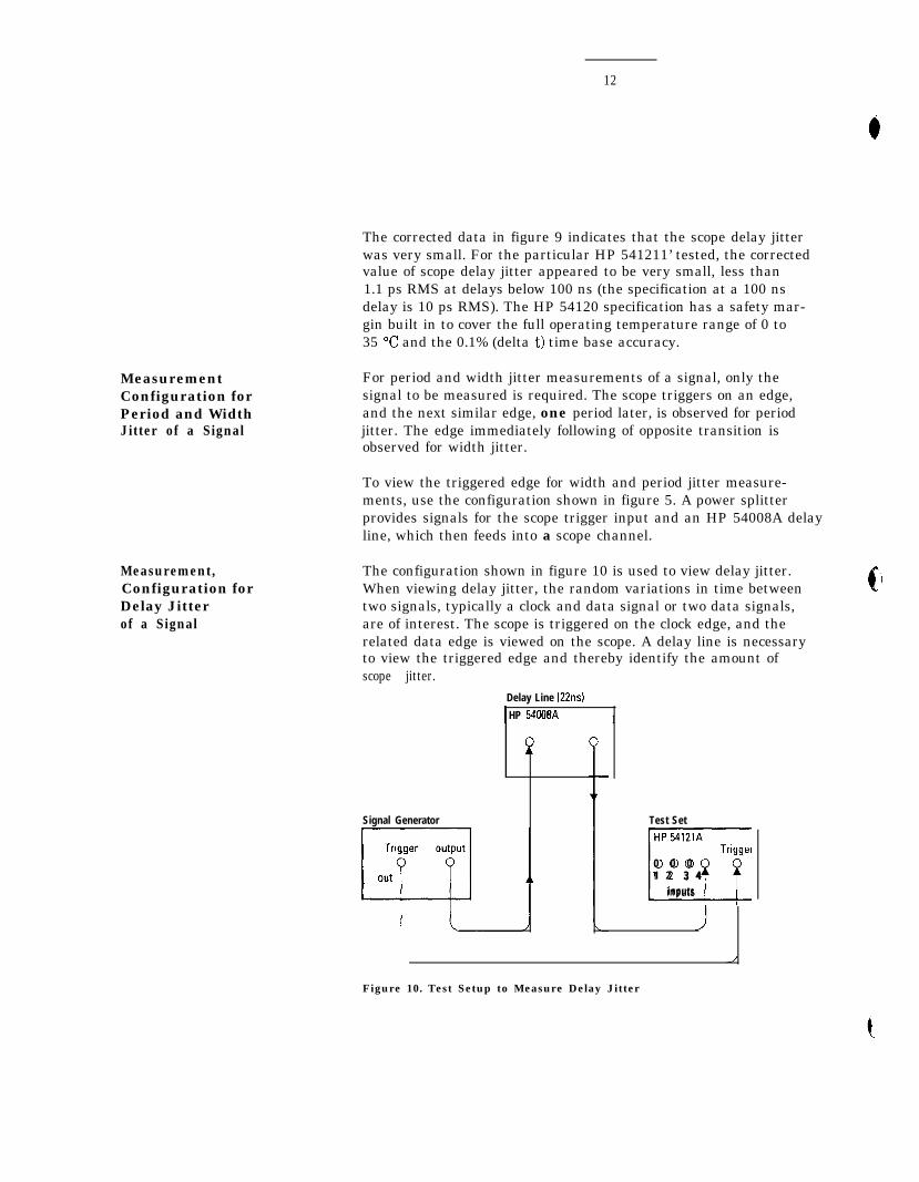
The corrected data in figure 9 indicates that the scope delay jitterwas very small. For the particular HP 541211’ tested, the correctedvalue of scope delay jitter appeared to be very small, less than1.1 ps RMS at delays below 100 ns (the specification at a 100 nsdelay is 10 ps RMS). The HP 54120 specification has a safety mar-gin built in to cover the full operating temperature range of 0 to35 “C and the 0.1% (delta t) time base accuracy.

For period and width jitter measurements of a signal, only thesignal to be measured is required. The scope triggers on an edge,and the next similar edge, one period later, is observed for periodjitter. The edge immediately following of opposite transition isobserved for width jitter.

To view the triggered edge for width and period jitter measure-ments, use the configuration shown in figure 5. A power splitterprovides signals for the scope trigger input and an HP 54008A delayline, which then feeds into a scope channel.

The configuration shown in figure 10 is used to view delay jitter.When viewing delay jitter, the random variations in time betweentwo signals, typically a clock and data signal or two data signals,are of interest. The scope is triggered on the clock edge, and therelated data edge is viewed on the scope. A delay line is necessaryto view the triggered edge and thereby identify the amount ofscope jitter.

Signal Generator

Delay Line (22ns)

1 HP 54008A I

P

Test SetHP 54121A

Triggel

i

0 0 01 2 3 4

i n p u t s

Figure 10. Test Setup to Measure Delay Jitter

13

JitterMeasurementon an ExampleSignal

Measurement ofPeriod andWidth Jitter

Typical HP 54120 performance data presented in this note is usefulfor rough estimates of measurement feasibility. Actual measure-ments of scope induced jitter should be made on the scope to be usedin a measurement. The measurement for scope trigger threshold jit-ter should be performed using the actual trigger edge available inthe real measurement. The amount of oscilloscope time base delayjitter should be determined from measurements with a stablesource. Characterization of an individual scope’s time base delayjitter can be performed once and retained for reference in anymeasurement.

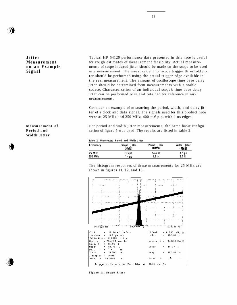
Consider an example of measuring the period, width, and delay jit-ter of a clock and data signal. The signals used for this product notewere at 25 MHz and 250 MHz, 400 mV p-p, with 1 ns edges.

For period and width jitter measurements, the same basic configu-ration of figure 5 was used. The results are listed in table 2.

Table 2. Uncorrected Period and Width Jitter

Frequency Scope Jitter Period Jitter Width JitterMlSI WtMS) MJlSI

25 MHz250 MHz

1 . 5 p s1.4rls

1 4 . 4 p s4.2 DS

1 . 5 p s2 . 7 D S

The histogram responses of these measurements for 25 MHz areshown in figures 11, 12, and 13.

19.8830 n5 19.9330 ns

Ch.4 = 10.00 mUolts/dlv Clffsei = 8.750 mUoltsrImebase - 10.0 pr/dlv Deldy = 19.5530 rl5

'Delta Wlndo- 0.0000 UollsWlndow I s 9.2750 mUoit5 Wlndow 1 = 9.3750 mvo1tsDelta % - 65.95 %UPPW = 84.75 % Lower = 18.77 %Delta T = 2.Y PSstart - 19.5863 "5 stop = 19.5533 rl5x Samples = 10000Mean * 19.5946 "5 SiQ,,a = 1.5 PS

Trigger on Erternal at Pos. Edge st Il.00 muoit5

Figure 11. Scope Jitter

1 4

C h.4 = 1 0 . 0 0 mllolts/dlvT imebase = 1 0 . 0 ps/divll clta WIndo= 0 . 0 0 0 0 VoltsW Indow I - 3.3750 muo1ts0 eita % = 6 8 . 0 5 %U pper = 84.51 %D elta T = 15. I PSs tart - 39.9345 “5P Samples - / 0000M =a” s 39.9:69 “5

Offset = 8 . 7 5 0 mVoltsDelay = 39.9230 “5

W,“dOU ? = 9.3750 muo1t

Lower = 1 6 . 4 5 %

stop = 39.9194 “5

SlQrn.3 = 7.5 P5

Trlggcr on E.ternal a t Pas. E d g e a t 11.00 mvo1ts

Figure 12. Width Jitter

53.4330 “5 59.9330 “5

h.4 = :0.00 muolts/dli Offset = 8 . 7 5 0 mUott:lmebase = 5 0 . 0 psidlv Oelay = 59.6830 “ 5elta Wlndo- 0 . 0 0 0 0 V o l t sindow I = 9.3750 mva1ts W‘ndow 2 = 9.3750 muo1ie1ta % = 6 6 . 2 8 %PPer = 8 3 . 9 0 % iauer = 17.61 %elta T - 28.9 pstar t = 5 9 . 7 0 2 4 ns stop = 59.6716 “5

Samples = I0000can = 5 9 . 6 8 8 0 r5 51qma = 14.4 P5

TriQQer o n Ecternal a t Pas. E d g e a t I I . 0 0 muo1ts

i s

Figure 13. Period Jitter

t

15

Measurement ofDelay Jitter

Correcting forScope Error

Consider the measurement of delay jitter between the clock outputof the signal generator and data output at 25 MHz. On this particu-lar device under test (DUT), there was a fixed delay between clockand data, and an additional delay up to one period could be added.

Scope trigger threshold jitter was determined by looking at the trig-gered edge of the DUT clock output. The measurement was per-formed by replacing the data input to the power splitter in the con-figuration shown in figure 5 with the DUT clock output. Scope jitterwas measured as 1.6 ps.

Next, the delay line was removed, the clock was fed into the scopetrigger input, and the delay line was inserted between the data out-put and the scope input, as shown in figure 10.

Jitter was measured on the delayed data edge, both at a minimumdelay setting and maximum delay setting on the DUT. The uncor-rected measured jitter results were 2.9 ps and 19.4 ps respectively.

At this point, the scope jitter has been identified, although it isstill part of the measurement. Now an approach will be outlinedwhich quantifies the error caused by scope jitter and partiallycorrects for it.

If Y is a sum of random variables Xl and X2, and these randomvariables are uncorrelated (one does not affect the other),

Then

the mean of Y = E(Y) = E(X1) + E(X.2)

which is the sum of the means of Xl and X2.

And

the variance of Y = (~~2 = ai2 + ~~2.

Therefore the variances add directly. (1)

If the variances add, since the variance equals the square of thestandard deviation, then this implies that the standard deviationsof two normal uncorrelated distributions add via a quadratic equa-tion. Thus, the standard deviation is the square root of the sum ofthe squares.

16

Therefore, for uncorrelated scope jitter and signal jitter,

Signal Jitter (actual) = j/ Fd/- [tg;d[- [tii;e)

where jitter for each term is RMS.

In the example with the 25 MHz square wave, the scope jitter wasmeasured at 1.5 ps, and measured period jitter of 14.4 ps.

Period Jitter (actual) = 1’(14.4)2- (1.51)~ = 14.3~s

Recall that at the scope delays used to measure period and widthjitter in this example (39.9 ns and 59.7 ns beyond triggered edge)scope time base delay jitter was hardly measurable. Therefore, onlythe trigger threshold jitter was important for this calculation. Inthis case, scope trigger threshold jitter caused only a 0.6% error.In general, if the scope jitter is less than three times the jitter to bemeasured, the scope error contribution should be less than 5.0%,since jitter adds via a quadratic equation. Keeping this 3:l marginbetween signal jitter and scope jitter is a good rule of thumb, whichwill reduce the need to back out scope induced error.

Table 3 shows the corrected results of the example DUT measure-ments after backing out the scope jitter.

TABLE 3. Corrected DUT Jitter

Frequency Period

25 MHz 1 4 . 3 ps

Width Delay (+ll)

7.3 PS 2.4 OS

Delay (+49 ns)

19.3 OS250 MHz 4.0 is 2.3 is not taken not taken

Instructions forMeasuring Jitter

Width and PeriodJitter Measurements

17

This section will provide step-by-step procedures for measuringwidth, period, and delay jitter. To supplement these procedures,section 3 of the Getting Started Guide for the HP 54121T Digitiz-ing Oscilloscope provides step-by-step procedures for histogrammeasurements.

The procedures for measuring width and period jitter are as follows:

1) Connect your equipment as shown in figure 5, with your signalto be measured replacing the signal generator.

2) Select Autoscale on your HP 54120.

3) Determine which edge is the triggered edge by varying thefrequency of the source and observing that the triggered edgeremains stationary. Or, if the amount of delay in the signal path isknown, set the center of the scope time base delay to the value ofthe delay.

4) Expand the scope time/div until the edge spans the entirescreen. Keep the edge centered on the screen with the oscilloscopetime base delay setting.

5) If needed, expand the scope volts/div to obtain a minimum ofone-half a major division of jitter. See figure 6a for an example of aproper display of jitter.

6) Select the histogram menu on the HP 54120. Obtain a time his-togram with the windowed area at the center of the edge. If an hourglass is apparent, window at the center of the it for scope triggerthreshold jitter only. Window off the hour glass for a measurementof trigger threshold and signal noise jitter. (See figure 6a.) Thewindow markers should be on top of one another so that the deltawindow is 0.0 V.

7) Set the number of samples to be acquired to a minimum of 500.Acquire the statistical data, by pushing the Acquire button.

8) Select results and then select sigma. The statistical results ofthe data will be displayed at the bottom of the screen. Record sigmafor use in calculations later. This value of sigma is the scope triggerthreshold jitter, when measured at the center of the hour glass ifpresent.

9) To measure width jitter, increase the scope time base delay toview the next edge of opposite polarity. Measure width jitter in thesame manner that the jitter on the triggered edge was measured.See steps 6 - 8. Record the measured width jitter.

18

Delay JitterMeasurements

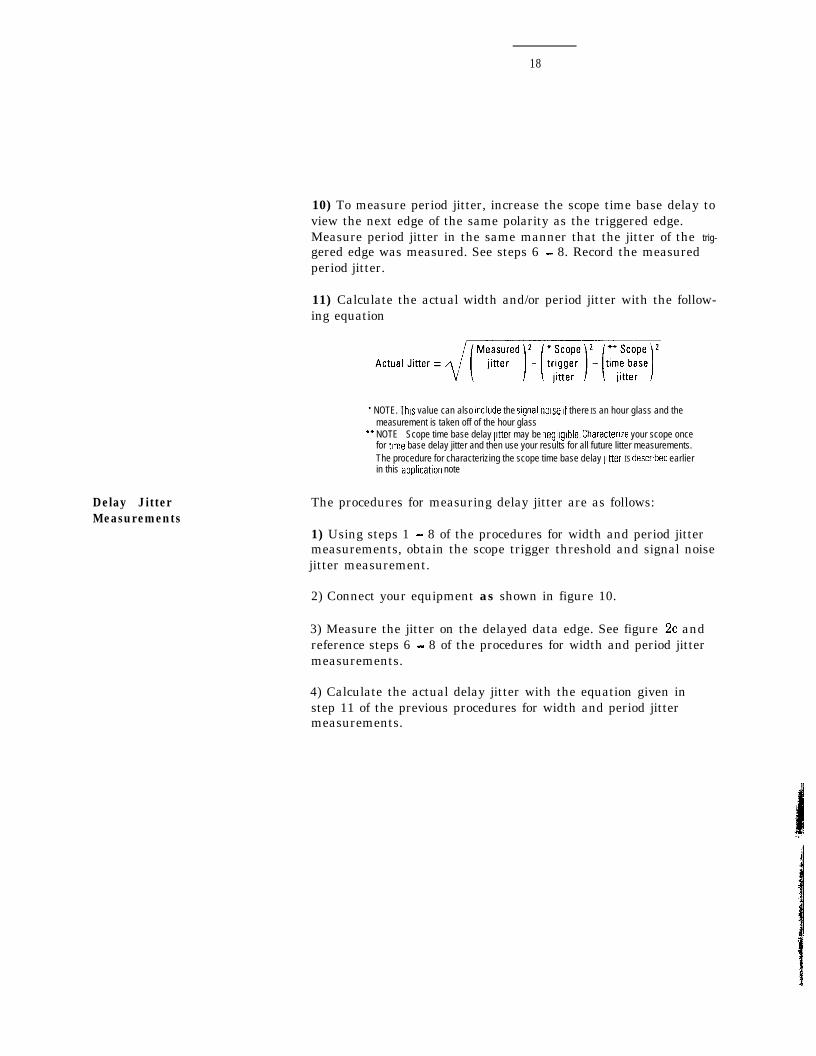
10) To measure period jitter, increase the scope time base delay toview the next edge of the same polarity as the triggered edge.Measure period jitter in the same manner that the jitter of the trig-gered edge was measured. See steps 6 - 8. Record the measuredperiod jitter.

11) Calculate the actual width and/or period jitter with the follow-ing equation

* NOTE. Thus value can also mclude the signal norse If there IS an hour glass and themeasurement is taken off of the hour glass

‘* NOTE Scope time base delay $ter may be neglrgrble. Characterize your scope oncefor trme base delay jitter and then use your results for all future litter measurements.The procedure for characterizing the scope time base delay ytter IS described earlierin this applrcatron note

The procedures for measuring delay jitter are as follows:

1) Using steps 1 - 8 of the procedures for width and period jittermeasurements, obtain the scope trigger threshold and signal noisejitter measurement.

2) Connect your equipment as shown in figure 10.

3) Measure the jitter on the delayed data edge. See figure 2c andreference steps 6 - 8 of the procedures for width and period jittermeasurements.

4) Calculate the actual delay jitter with the equation given instep 11 of the previous procedures for width and period jittermeasurements.

19

Improving theThroughputof JitterMeasurements

For some applications it may be desirable to decrease the time tocollect the data samples used in jitter measurements. Whenincreased throughput is needed, it can be obtained with a trade offof measurement accuracy for decreased acquisition time.

Rather than place the window markers for a delta voltage of 0.0 V,as in step 6 of the width and period jitter measurement instructionsgiven earlier in this publication, select a larger window. The largerthe window the more error introduced into the measurement. Tocompensate for the error in the measured jitter with a windowgreater than 0.0 V, the slope of the edge being measured must beknown. The following formula can be used to minimizemeasured error:

The measurement of the slope should be from the center of the edge.The accuracy of the slope measurement is proportional to the accu-racy of the calculated jitter. Larger windows allow data to be col-lected in less time at the cost of additional measurement error, indi-vidual users should determine the most desirable combination ofthroughput and accuracy for their applications.

(Reference Meyer, page 126, example 7.18)

20

Conclusions: l For greatest accuracy in jitter measurements, individualoscilloscopes need to be characterized prior to making jitter mea-surements. Simple techniques, described in this paper, can be usedto identify scope jitter in a measurement and separate scope jitterfrom the measured jitter of a signal. When the scope jitter is uncor-related to the measured signal jitter, scope and signal jitter add asthe square root of the sum of the squares. Thus, one should eitherensure that scope jitter is small compared to the jitter of interest(perhaps 3 times smaller) or mathematically remove the effect ofscope jitter on the measurement.

l Slew rate and noise on a trigger edge significantly effect scope trig-ger threshold jitter. Considering measurements of 0.6 ps (RMS)scope jitter best case, measurements of jitter as small as 1.8 psshould be possible on fast slew rate signals. Signals with slowerslew rates cause increased scope trigger threshold jitter. Theamount of jitter should be measured to determine its effect on ameasurement.

l Higher amplitude signals produce less trigger threshold jitter. Thus,scope trigger threshold jitter can be reduced by amplifying the sig-nal to be measured. The amplifier must not have excessive noisewhich counteracts the benefits of amplification.

l Scope time base delay jitter can be a factor in jitter measurements.By specification, total jitter can be 5 ps + (5x10-5 x scope delay set-ting). However, for many measurements, particularly at delays lessthan 60 ns, scope time base delay jitter may be negligible

21

Basics of Statistics

le.

Appendix A:Statistical Analysisof Signals andHistograms

The purpose of this appendix is to provide an over view of thestatistical analysis used in the HP 54120 family of oscilloscopesand to provide an understanding of the formation of histograms.

This appendix contains excerpts from HP Product Note 54120-1,“Histograms and Statistical Analysis of Signals For Use WithHP 54120 Digitizing Oscilloscope.”

The sample mean, denoted %, is the most common way of measur-ing the center of a set of data. Equation 1 defines the mean as

Equation 1.i=l

Note that z is an unbiased estimator of the true mean of the popu-lation, p (mu). Therefore, the sample mean approaches the truemean for a large sample number, n.

The sample standard deviation, denoted CX, is a measure of theextent to which the data points deviate from the mean. Equation 2is the definition of cr.

Equation 2.

0 is a biased estimator of the true standard deviation, CJ (sigma) ofthe entire population. For a large sample, G is commonly used toestimate sigma.

Another statistical value of concern is the root-mean-square (RMS).Equation 3 is the definition of RMS. The RMS value and sigmaapproach the same value as the number of samples increases. TheRMS value for a normal distribution, to be discussed next, isone sigma.

r.-----i--

Equation 3.

RMS=I/ (‘/,I CXi’i-1

22

B

The normal distribution, the bell-shaped curve, and the Gaussiandistribution all describe the distribution shown in figure Al. Thedistribution is symmetric about the mean and the shape of the dis-tribution is a function of the standard deviation. Equation 4 definesthe Gaussian distribution.

Equation 4.

x(mean)

Outcome

Figure Al. The Normal Distribution

In a normal distribution, the area under the curve to the right ofthe positive one standard deviation (sigma) point is 15.8% of thetotal area under the curve. Therefore the area under the curvebounded by the one standard deviation points is 68.26% of the total.Similarly, the area bounded by the two and three standard devia-tion points is 95.44% and 99.74% respectively.

3 2 -1 0 1 2 3

-68.26% -

1 95.44% (

I 99.74% I

Figure A2. Area Bounded by no

23

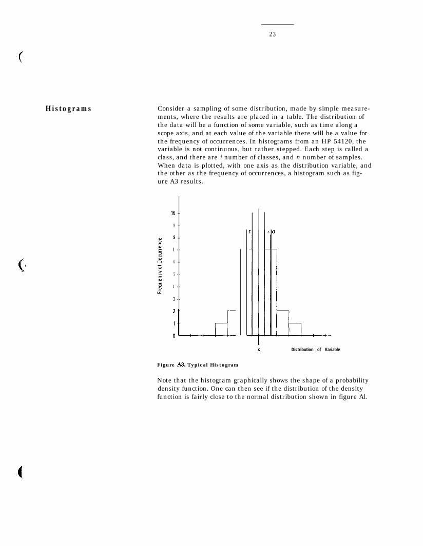
Histograms Consider a sampling of some distribution, made by simple measure-ments, where the results are placed in a table. The distribution ofthe data will be a function of some variable, such as time along ascope axis, and at each value of the variable there will be a value forthe frequency of occurrences. In histograms from an HP 54120, thevariable is not continuous, but rather stepped. Each step is called aclass, and there are i number of classes, and n number of samples.When data is plotted, with one axis as the distribution variable, andthe other as the frequency of occurrences, a histogram such as fig-ure A3 results.

I O - -

9 - -

a - -

I - -

6 - -

5 - -

4 - -

3 --

Figure A3. Typical Histogram

Distribution of Variable

Note that the histogram graphically shows the shape of a probabilitydensity function. One can then see if the distribution of the densityfunction is fairly close to the normal distribution shown in figure Al.

24

The DigitizingScope HistogramRepresentationWith Mean andStandard Deviation:

Using the Histogram menu on an HP 54120 digitizing oscilloscope,a voltage slice is selected, the data points are collected, and ahistogram is displayed. An example histogram taken with 1,000samples is shown in figure A4. Notice that the percentage of hitsabout the mean indicate a fairly normal distribution. The mean andsigma of the distribution can also be determined from the datapoints and are available at the push of the Sigma button on theHP 54120 histogram menu.

CT0W0UDStM

h.4 =*mebase =e1ta Windo=rndaw I *e1ta % -PPer =elta T -tart =Samples =

can =

20.00 mVolts/div5 0 . 0 ps/d,v0 . 0 0 0 0 Volt59 . 3 7 5 0 nuoits66.28 %85.90 %29.959.7024 ::I0000

5 9 . 6 8 8 0 ns

L‘5 53.9::0 n5

Offset = R . 7 5 0 mVoltsDelay = 59.6830 “5

W,ndow 2 = 9.:750 mua1t,

Lauer = 17.61 %

stop = 59.6736 n5

S1gna = 14.4 ps

Tr,gger on E.ternal a t P a s . Edge a t I l . 0 0 nuo1ts

5

Figure A4. Digitizing Oscilloscope Histogram Measurement

i Q

25

I .ci

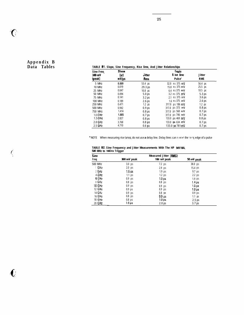
Appendix BData Tables TABLE El. Slope, Sine Frequency, Rise lime, And Jitter Relationships

Sine Freo Slooe Equiv3lHlmV ’(peak)

5 MHz10 MHz25 MHz50 MHz75 MHz

100 MHz250 MHz500 MHz750 MHz

1.0 GHz1.5 GHz2.0 GHz

br)mV/ps0.009

R i& lime JitterPulse’ RMS

0.0190.0470.0940.1410.1890.4710.9421.4141.8852.8273.768

53.4 ps 32.0 n s 375 mV 56.4 ps29.3 ps 15.8 n s 375 mV 25.5 ps10.8 ps 6.4 n s 375 mV 10.5 ps5.0 ps 3.2 n s 375 mV 5.3 ps3.2 ps 2.1 n s 375 mV 3.6 ps2.6 ps 1.6 n s 375 mV 2.6 ps1.2 ps 317.0 p s 186 mV 1.2 ps0.9 ps 317.0 p s 373 mV 0.8 ps0.8 ps 317.0 p s 560 mV 0.7 ps0.7 ps 317.0 p s 746 mV 0.7 ps0.8 ps 133.0 ps 469 mV 0.8 ps0.8 PS 133.0 DS 634 mV 0.7 ps

0.7 ps2.5 GHz 4.710 0.6 bs 133.0 bs 781 mV

* NOTE When measuring rise times. do not use a delay line. Delay lines can distort the rismg edge of a pulse

TABLE 82. Sine Frequency and Jitter Measurements With The HP 54118A,500 MHz to 1gGHz Trigger

Freq

500 MHz1 GHz2 GHz4 GHz6GHz8 GHz

10 GHz12 GHz14 GHz16 GHz18 GHz20 GHz -

300 mV peak

3.0 p s2.0 p s1.6~s1.1 p s0.9 p s0.8 p s0.9 p s0.9 p s0.9 p s0.8 p s0.8 p sl.Ops

Measured Jitter (RMS)1M) mV peak

7.2 p s2.9 p s1.9 p s1.2 p sl.Ops0.8 p s0.9 p s0.9 p s0.8 OS

50 mV peak38.0 p s15.4 p s

9.7 p s2.2 p s1.9 p s1.4psl.Opsl.Ops0.9 p s1.1 ps2.5 ps3.7 ps

0.9 bsl.Ops2.0 ps

26

References Hewlett-Packard Co. 1988. Histograms and Statistical Analysis ofSignals for Use With HP 54120 Digitizing Oscilloscope. HewlettPackard Product Note 54120-l.

Hewlett-Packard Co. 1987. HP 5370. Frequency and Time IntervalAnalyzer, Jitter and Wander Analysis in Digital Communications.Hewlett Packard Application Note 358-2.

Hewlett Packard Getting Started Guide for the HP 54121T. 1988.

Hogg, Robert V. and Tanis, Elliot A. Probability and StatisticalInference, page 145.

Meyer, Paul L. 1966. Introductory Probability and StatisticalApplications. Reading, Massachusetts, Addison-WesleyPublishing Company. pp 124-126.

Papoulis, Athanasios 1984. Probability, Random Variables, andStochastic Processes. New York, McGraw-Hill Book Company.pp 152-153.

HEWLETTPACKARD

United States:Hewlett-Packard Company4 Choke Cherry RoadRockville, MD 20850(301) 670-4300

Hewlett-Packard Company5201 Tollview DriveRolling Meadows, IL 60008(312) 255-9800

Hewlett-Packard Company5161 Lankershim Blvd.No. Hollywood, CA 91601(818) 5055600

Hewlett-Packard Company2015 South Park PlaceAtlanta, GA 30339(404) 955-1500

Canada:Hewlett-Packard Ltd.6877 Goreway DriveMississauga, Ontario L4VlM8(416) 678-9430

European Headquaters:Hewlett-Packard S. A.150, Route du Nant d’Avril12 17 Meryin 2Geneva--Switzerland41/22 780-8111

Japan:Yokogawa-Hewlett-Packard Ltd.29-21, Takaido-Higashi 3-chomeSuainami-ku, Tokyo 168(035 331-6111

Latin America:Latin American Region HeadquartersMonte Pelvoux Nbr. 111Lomas de Chapultapec11000 Mexico, D.F. Mexico(905) 202-0155

Australia/New Zealand:Hewlett-Packard Australia Ltd.31-41 Joseph StreetBlackburn, Victoria 3130Melbourne, Australia(03) 895-2895

Far East:Hewlett-Packard Asia Ltd.22/F Bond Centre, West Tower89 Queensway, Central, Hong Kong(5) 848-7777

Printed in U.S.A. 9189.5952-7085