http://www.isis.ecs.soton.ac.uk

Sparse Kernels MethodsSparse Kernels Methods

Steve Gunn

OverviewOverview

Part I : Introduction to Kernel Methods

Part II : Sparse Kernel Methods

Part IPart I

Introduction to

Kernel Methods

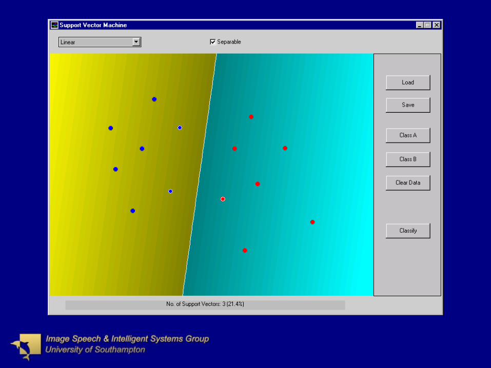
ClassificationClassification

Consider 2 class problem

f x

1

1

Class A

Class B

Optimal Separating HyperplaneOptimal Separating Hyperplane

Optimal Separating HyperplaneOptimal Separating Hyperplane

y y R yl ln

1 1 1 1, , , , , , ,x x x

w x b 0

Separate the data,

with a hyperplane,

such that the data is separated without error, and the distance

between the closest vector to the hyperplane is maximal.

SolutionSolution

w w w 1

2

The optimal hyperplane minimises,

subject to the constraints,

y b i li iw x 1 1, , ,

and is obtained by finding the saddle point of the Lagrange functional

L b b yi ii

l

w w w x w, , 1

21

1

Finding the OSHFinding the OSH

Size is dependent upon training set size

Unique global minimum

min

1

2T TH c

Quadratic Programming Problem

TiY i l 0 0 1, , , , .

Support VectorsSupport Vectors

Information contained in support vectors

Can throw away rest of training data

SVs have non zero Lagrange multipliers

Generalised Separating HyperplaneGeneralised Separating Hyperplane

Non Separable CaseNon Separable Case

Introduce slack Variables

y b i li i iw x 1 1 , , ,

w w w, 1

2 1

C ii

l

Minimise

C is chosen a priori

and determines trade-off to non-separable case.

Size is dependent upon training set size

Unique global minimum

min

1

2T TH c

Quadratic Programming Problem

0 1

01

i

i ii

l

C i l

y

, , ,

.

Finding the GSHFinding the GSH

Non-Linear SVMNon-Linear SVM

Map input space to high dimensional feature space

Find OSH or GSH in Feature Space

Kernel FunctionsKernel Functions

Hilbert Schmidt Theory

Mercer’s Conditions

K x x k x k xi j i j,

K x x x x

K x x g x g x dx dx g x dx

i j m i jm

m

i j i j i j i i

, ,

, ,

1

2

0

0

K x xi j, is a symmetric function

Polynomial Degree 2Polynomial Degree 2

k

x

x

x

x

x x

Kx x y x y

1

2

2

2

1

1

2

12

22

1 2

2,

K k kx y x y,

Acceptable Kernel FunctionsAcceptable Kernel Functions

Polynomial

Multi-Layer Perceptrons

Radial Basis Functions

K x x x x

K x x x xd

i j i j

d

i j i j

d

,

,, ,...

11

K x x

x xi j

i j, exp

2

2

K x x b x x ci j i j, tanh

Iris Data SetIris Data Set

RegressionRegression

Approximation Error

Model Size

Generalisation

Estimation Error

RegressionRegression

y y R y Rl ln

1 1, , , , , ,x x x

Approximate the data,

with a hyperplane,

and the SRM principle.

f x b, w x

w w cn

using a loss function, e.g.,

L y f a y f a, , ,x x

SolutionSolution

w w w, ,* *

1

2 1 1

C ii

l

ii

l

w x

w x

i i i

i i i

i

i

b y

b yi l

*

*,...,

0

0

1

Introduce slack variables and minimise

subject to the constraints

Finding the SolutionFinding the Solution

Size is dependent upon training set size

Unique global minimum

Quadratic Programming Problem

0 1

0 1

01

i

i

i ii

l

C i l

C i l

, , ,

, , , .*

*

minx

T Tx Hx c x1

2 x

*

where

Part I : SummaryPart I : Summary

Unique Global Minimum

Addresses Curse of Dimensionality

Complexity dependent upon data set size

Information contained in Support Vectors

Part IIPart II

Sparse Kernel Methods

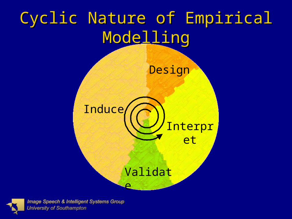
Cyclic Nature of Empirical ModellingCyclic Nature of Empirical Modelling

Induce

Validate

Interpret

Design

InductionSVMs have strong theory

Good empirical performance

Solution of the form,

InterpretationInput Selection

Transparency

SVs

,xxx iiKf

Additive RepresentationAdditive Representation

f f f x f x x fi ii

n

i j i jj i

n

i

n

n( ) ,, , , ,x x 0

1 111 2 ...

Additive structure

Transparent

Rejection of redundant inputs

Unique decomposition

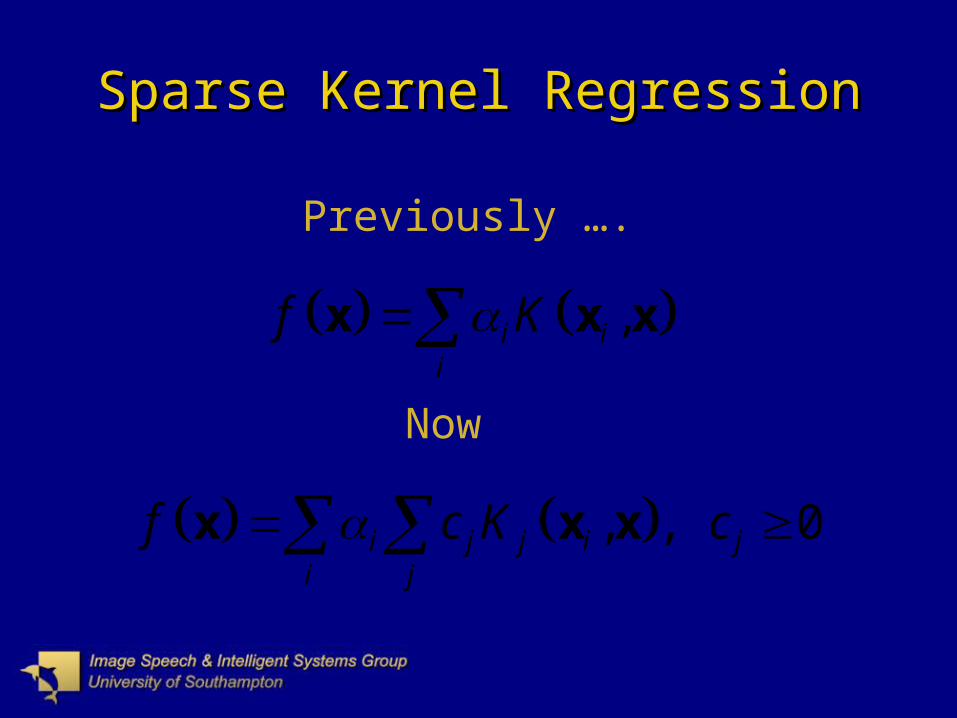
Sparse Kernel RegressionSparse Kernel Regression

, , 0i j j i ji j

f c K c x x x

,i ii

f Kx x x

Previously ….

Now

The PriorsThe Priors

“Different priors for different parameters”

Smoothness – controls “overfitting”

Sparseness – enables input selection and controls overfitting

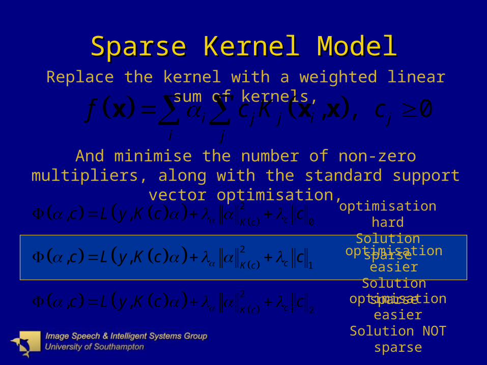
Sparse Kernel ModelSparse Kernel Model

2

0, , cK cc L y K c c

Replace the kernel with a weighted linear sum of kernels,

And minimise the number of non-zero multipliers, along with the standard support vector optimisation,

optimisation hardSolution sparse

2

1, , cK cc L y K c c

2

2, , cK cc L y K c c

optimisation easierSolution sparse

optimisation easierSolution NOT sparse

, , 0i j j i ji j

f c K c x x x

Choosing the Sub-KernelsChoosing the Sub-Kernels

• Avoid additional parameters if possible

• Sub-models should be flexible

Spline KernelSpline Kernel

dttvtuuvvukspline 1

01,

3,min6

1,min

21, vuvu

uvuvvukspline

Tensor Product SplinesTensor Product Splines

n

d

ddANOVA vukvuK

1

,1,

),(),(),(),(1),(1 221122112

1

vukvukvukvukvukd

dd

3,min6

1,min

2, vuvu

uvuvvuk

The univariate spline which passes through the origin has a kernel of the form,

E.g. for a two input problem the ANOVA kernel is given by

And the multivariate ANOVA kernel is given by

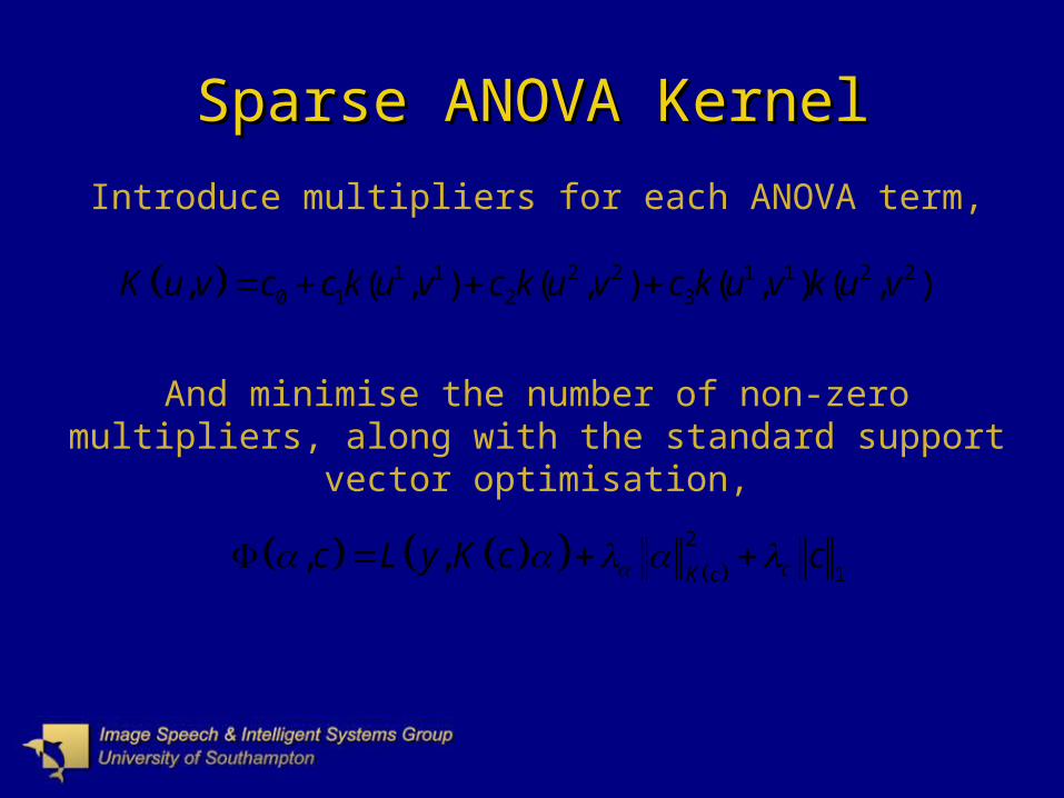
Sparse ANOVA KernelSparse ANOVA Kernel

1 1 2 2 1 1 2 20 1 2 3, ( , ) ( , ) ( , ) ( , )K u v c c k u v c k u v c k u v k u v

Introduce multipliers for each ANOVA term,

And minimise the number of non-zero multipliers, along with the standard support vector optimisation,

2

1, , cK cc L y K c c

OptimisationOptimisation

Quadratic LossQuadratic Loss

Epsilon-Insensitive LossEpsilon-Insensitive Loss

AlgorithmAlgorithm

ModelSparse ANOVA

Selection

ParameterSelection

Data

ANOVA BasisSelection

3+ Stage Technique

Each stage consists of solving a convex, constrained optimisation problem. (QP or LP)

Auto-selection of Parameters

Capacity Control Parametercross-validation

Sparseness ParameterValidation error Stage I

Sparse Basis SolutionSparse Basis Solution

0subject tomin1

2

2 i

ccccy

0subject to21min iTTT

cccycc

0subject tomin1,1

i

ccccy

.0

,0

,0

,subject to

1

1

1

min

j

j

i

T

n

m

c

y

y

n

m

c

II

II

n

m

c

c

Quadratic Loss Function (Quadratic Program)

-Insensitive Loss Function (Linear Program)

AMPG ProblemAMPG Problem

Predict automobile MPG (392 samples)

Inputs:no. of cylinders, displacement

horsepower, weight

acceleration, year

Output: MPG

60 80 100 120 140 160 180 200 220-7

-6

-5

-4

-3

-2

-1

0

Horse Power

MP

G

2000 2500 3000 3500 4000 4500 5000-14

-12

-10

-8

-6

-4

-2

0

Weight

MP

G

70 72 74 76 78 80 82-1

0

1

2

3

4

5

6

7

8

9

Year

MP

G

Horse Power 50 86 122

Horse Power 158 194 230

Network transparency through ANOVA representation.

SUPANOVA AMPG Results (SUPANOVA AMPG Results (=2.5)=2.5)

Loss Function Estimated Generalisation Error

Stage I Stage III Linear ModelTraining Testing

Mean Variance Mean Variance Mean Variance

Quadratic Quadratic 6.97 7.39 7.08 6.19 11.4 11.0

Insensitive Insensitive 0.48 0.04 0.49 0.03 1.80 0.11

Quadratic Insensitive 1.10 0.07 1.37 0.10

Insensitive Quadratic 7.07 6.52 7.13 6.04 11.72 10.94

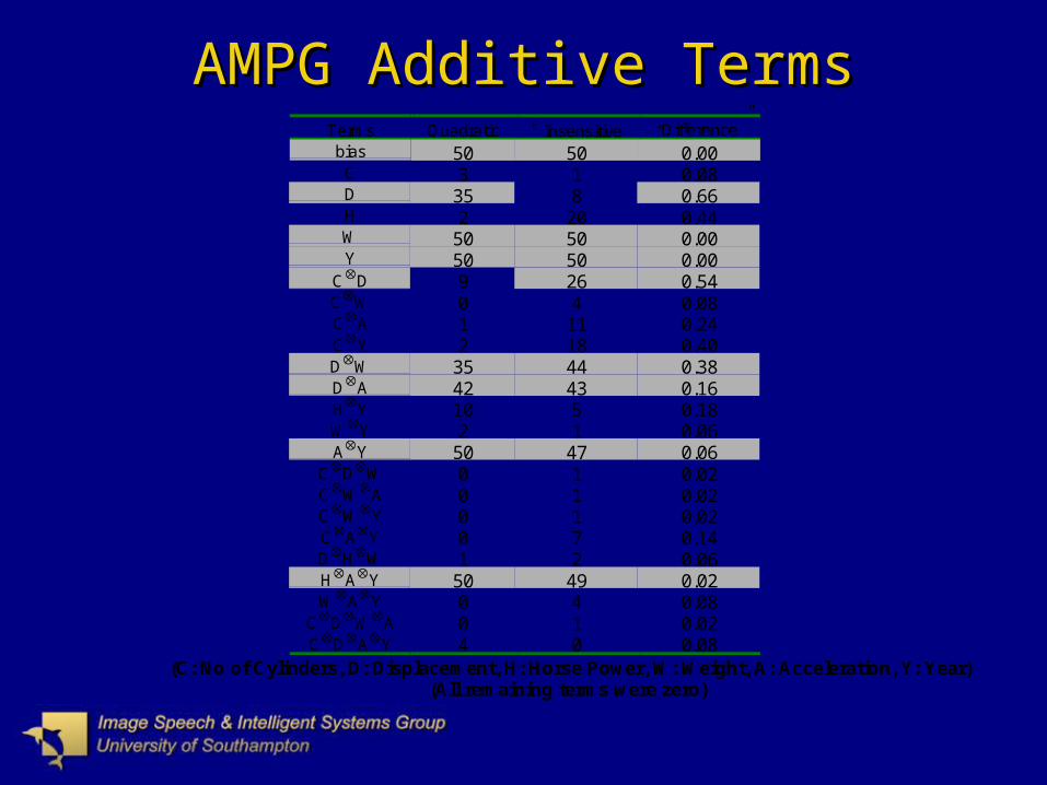
AMPG Additive TermsAMPG Additive TermsTerms Quadratic Insensitive “Difference”bias 50 50 0.00C 3 1 0.08D 35 8 0.66H 2 20 0.44W 50 50 0.00Y 50 50 0.00

CD 9 26 0.54CW 0 4 0.08CA 1 11 0.24CY 2 18 0.40DW 35 44 0.38DA 42 43 0.16HY 10 5 0.18WY 2 1 0.06AY 50 47 0.06

CDW 0 1 0.02CWA 0 1 0.02CWY 0 1 0.02CAY 0 7 0.14DHW 1 2 0.06HAY 50 49 0.02WAY 0 4 0.08

CDWA 0 1 0.02CDAY 4 0 0.08

(C: No of Cylinders, D: Displacement, H: Horse Power, W: Weight, A: Acceleration, Y: Year)(All remaining terms were zero)

SummarySummary

SUPANOVA is a global approach

Strong Basis (Kernel Methods)

Can control loss function and sparseness

Can impose limit on maximum variate terms

Generalisation + Transparency

Further InformationFurther Information

http://www.isis.ecs.soton.ac.uk/

isystems/kernel/

SVM Technical Report

MATLAB SVM Toolbox

Sparse Kernel Paper

These Slides