Rapp. P.-v. Réun. Cons. int. Explor. Mer, 189: 345-352. 1990

Hydroacoustic surveys of zooplankton biomass and distribution in the Beaufort Sea in 1985 and 1986

Gary E. Johnson and William B. Griffiths

Johnson, Gary E ., and Griffiths, William B. 1990. Hydroacoustic surveys of zoo­plankton biomass and distribution in the Beaufort Sea in 1985 and 1986. - Rapp. R-v. Réun. Cons. int. Explor. Mer, 189: 345-352.

The biomass and distribution of zooplankton, the primary food source of the bow- head whale, were surveyed in the Beaufort Sea in September 1985 and 1986. The surveys were part of a comprehensive two-year study of the use of the survey area for feeding by bowhead whales. During both years, simultaneous hydroacoustic and bongo-net plankton samples were obtained at stations between the 10- and 200-m isobaths. Continuous hydroacoustic data were collected along transects between the stations. A regression model of hydroacoustic volume scattering at 200 kHz vs. bongo-net biomass (mg m ' 3) was derived from data collected at the stations. Sep­arate models were used each year to predict zooplankton biomass from volume- scattering data collected along the transects.

Gary E. Johnson: BioSonics, Inc., 3670 Stone Way North, Seattle, Washington 98103, USA. William B. Griffiths: L G L Limited, Environmental Research Associates, 9768 2nd Street, Sidney, British Columbia, Canada V8L3Y8.

1. IntroductionThe objective of this paper is to present the methodol­ogy and some results of hydroacoustic surveys of zoo­plankton in the eastern Alaskan Beaufort Sea in 1985 and 1986. These surveys were part of a comprehensive study to determine what proportion of the energy re­quirements of the western Arctic bowhead whale (Ba- leana mysticetus) is obtained from zooplankton food resources located in the area. Since oil and gas devel­opment in this region could impact bowhead feed ing , a two-year study of bowhead feeding was conducted. The main objectives of the hydroacoustic work were:

(1) To determine a regression relationship between zooplankton-net sample biomass and acoustic vol­ume scattering, and use this regression to estimate zooplankton biomass from continuous acoustic samples along transects.

(2) To determine vertical and horizontal distributions of zooplankton biomass and zooplankton patchi­ness in areas where whales were observed feeding, and over the entire study area.

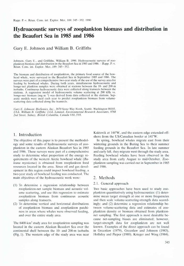
The 8400-km2 study area for zooplankton sampling was located in the eastern Alaskan Beaufort Sea over the continental shelf between the 10- and 200-m isobaths (Fig. 1). The western edge of the study area was near

Kaktovik at 144°W, and the eastern edge extended off­shore from the US/Canadian border at 141°W.

In spring, bowhead whales migrate east from their wintering grounds in the Bering Sea to their summer feeding grounds in the Beaufort Sea. In late summer and early fall, they migrate west through the study area. Feeding bowhead whales have been observed in the study area from early August to mid-October. Zoo­plankton sampling was carried out in September in 1985 and 1986.

2. Methods

2.1. General approach

Two basic approaches have been used to study zoo­plankton quantitatively using hydroacoustics: (1) deter­mine mean target strength at one or more frequencies and then scale volume-scattering-strength data accord­ingly; and (2) determine a regression relationship be­tween volume-scattering data and estimates of zoo­plankton density or biomass obtained from plankton- net sampling. The first approach is most desirable be­cause net-sampling biases are eliminated; however, target-strength data for zooplankton are not well known. Examples of the direct approach can be found in Greenlaw (1979), Greenlaw and Johnson (1983), Holliday and Pieper (1980), Krieger and Wing (1984),

345

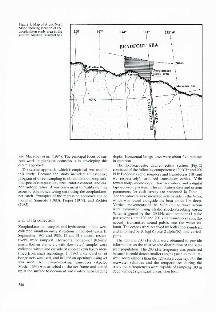
Figure 1. Map of Arctic North Slope showing location of the zooplankton study area in the eastern Alaskan Beaufort Sea.

15 0 ‘ 147' 144' 141 1 3 8 °W

BEAUFORT SEA

2 0 0 m

P r u d h o e Bay

Z ooplankton study areaKaktovil

M a c k e n z i e Bay

and Macauley et al. (1984). The principal focus of cur­rent work in plankton acoustics is in developing this direct approach.

The second approach, which is empirical, was used in this study. Because the study included an extensive program of direct sampling to obtain data on zooplank­ton species composition, sizes, caloric content, and car­bon isotope ratios, it was convenient to “calibrate” the acoustic volume-scattering data using the zooplankton- net catch. Examples of the regression approach can be found in Sameoto (1980), Pieper (1979), and Richter (1985).

2.2. Data collection

Zooplankton-net samples and hydroacoustic data were collected simultaneously at stations in the study area. In September 1985 and 1986, 11 and 31 stations, respec­tively, were sampled. Horizontal bongo-net (0.5-mm mesh, 0.61-m diameter, with flowmeter) samples were collected within and outside of zooplankton layers iden­tified from chart recordings. In 1985 a standard set of bongo nets was used, and in 1986 an opening/closing set was used. An upward-looking transducer (Apelco Model 1650) was attached to the net frame and aimed up at the surface to document and control net-sampling

depth. Horizontal bongo tows were about five minutes in duration.

The hydroacoustic data-collection system (Fig. 2) consisted of the following components: 120 kHz and 200 kHz BioSonics echo sounders and transducers (10° and 6°, respectively), armored transducer cables, V-fin towed body, oscilloscope, chart recorders, and a digital tape-recording system. The calibration data and system parameters for each survey are presented in Table 1. The transducers were mounted side by side in the V-fin, which was towed alongside the boat about 1 m deep. Vertical movements of the V-fin due to wave action were minimized using elastic shock-absorbing cords. When triggered by the 120 kHz echo sounder (1 pulse per second), the 120 and 200 kHz transducers simulta­neously transmitted sound pulses into the water co­lumn. The echoes were received by both echo sounders, and amplified by 20 log(R) plus 2 alpha(R) time-varied- gains.

The 120 and 200 kHz data were obtained to provide information on the relative size distribution of the sam­pled population. The 200 kHz frequency was preferred because it could detect smaller targets (such as medium­sized zooplankton) than the 120 kHz frequency. For the sea-water salinities and the temperatures during the study, both frequencies were capable of sampling 100 m deep without significant absorption loss.

346

V fin

200 kHz Transducer

EchoIntegrator

PortableComputer

ChartRecorder

ChartRecorder

200 kHz Echo

Sounder

120 kHz Echo

Sounder

Oscilloscope

DigitalRecording

System

y120 kHz

Transducer

Figure 2. Block diagram of the hydroacous­tic data-collection system used in the eastern Alaskan Beaufort Sea in September 1986.

2.3. Data analysis

2.3.1. Zooplankton-net-sample biomass The bongo-net catch was sorted to species or group, counted, and wet-weighed by taxon. After calculating the volume of water sampled (based on the flowmeter data) zooplankton biomass (mg m -3) for each tow was estimated by dividing sample wet-weight by volume of water sampled. In the case of copepods some subsam­pling was necessary. In these cases the samples were first scanned for large or rare animals, and then sub­

sampled with the Folsom plankton splitter (McEwen et a i , 1954). The subsampled copepods were counted, weighed to the nearest mg, and identified to species. The subsample data were then applied to the whole sample to estimate total wet-weight for each species. Total zooplankton biomass did not include detritus.

2.3.2. Echo integration and volume scattering Hydroacoustic volume-scattering data were obtained by processing digitized voltages with a BioSonics digital echo integrator. In 1985, integrator strata were 2 m

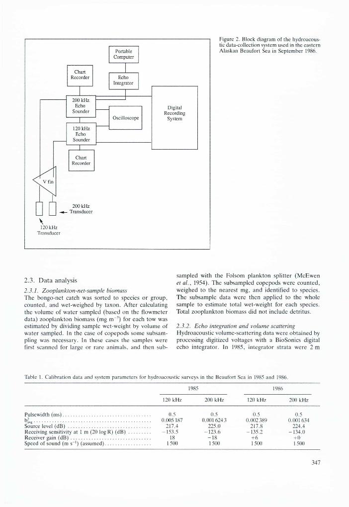
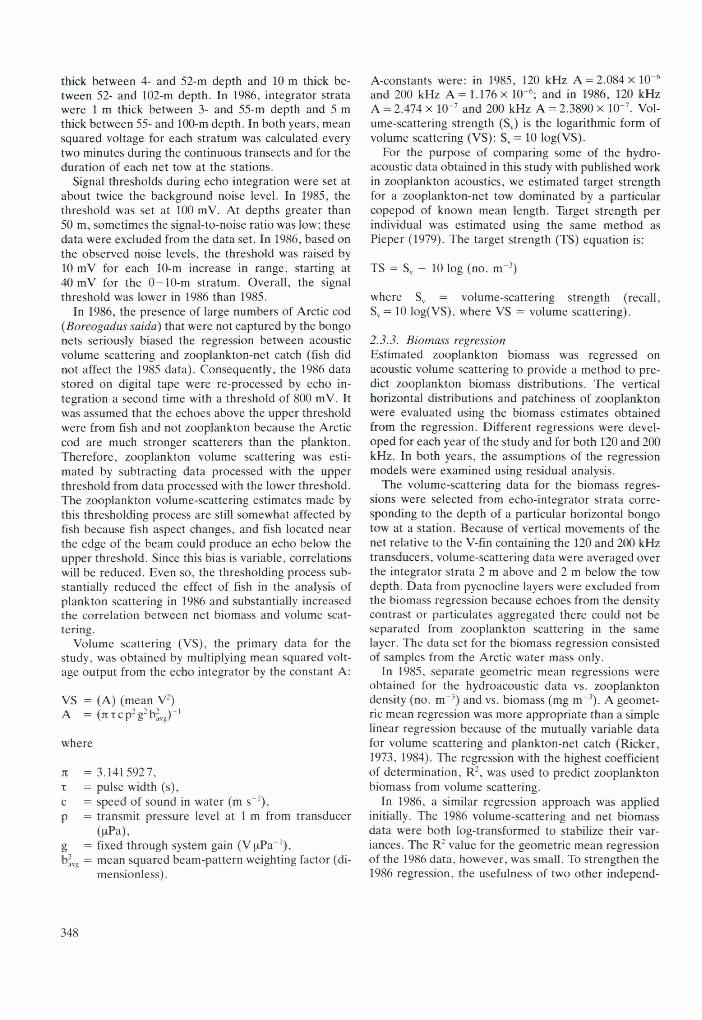
Table 1. Calibration data and system parameters for hydroacoustic surveys in the Beaufort Sea in 1985 and 1986.

1985 1986

120 kHz 200 kHz 120 kHz 200 kHz

Pulsewidth (m s) ....................................................u2

a v g ...........................................................................................................................................

Source level (dB) ...............................................Receiving sensitivity at 1 m (20 logR) (dB)Receiver gain ( d B ) .............................................Speed of sound (m s"1) (assumed).................

0.5 0.5 0.5 0.50.005187 0.0016243 0.002389 0.001634

217.4 225.0 217.8 224.4-153.5 -123 .6 -135 .2 -134 .0

18 - 1 8 +6 +01500 1500 1500 1500

347

thick between 4- and 52-m depth and 10 m thick be­tween 52- and 102-m depth. In 1986, integrator strata were 1 m thick between 3- and 55-m depth and 5 m thick between 55- and 100-m depth. In both years, mean squared voltage for each stratum was calculated every two minutes during the continuous transects and for the duration of each net tow at the stations.

Signal thresholds during echo integration were set at about twice the background noise level. In 1985, the threshold was set at 100 mV. At depths greater than 50 m, sometimes the signal-to-noise ratio was low; these data were excluded from the data set. In 1986, based on the observed noise levels, the threshold was raised by 10 mV for each 10-m increase in range, starting at 40 mV for the 0—10-m stratum. Overall, the signal threshold was lower in 1986 than 1985.

In 1986, the presence of large numbers of Arctic cod (Boreogadus saida) that were not captured by the bongo nets seriously biased the regression between acoustic volume scattering and zooplankton-net catch (fish did not affect the 1985 data). Consequently, the 1986 data stored on digital tape were re-processed by echo in­tegration a second time with a threshold of 800 mV. It was assumed that the echoes above the upper threshold were from fish and not zooplankton because the Arctic cod are much stronger scatterers than the plankton. Therefore, zooplankton volume scattering was esti­mated by subtracting data processed with the upper threshold from data processed with the lower threshold. The zooplankton volume-scattering estimates made by this thresholding process are still somewhat affected by fish because fish aspect changes, and fish located near the edge of the beam could produce an echo below the upper threshold. Since this bias is variable, correlations will be reduced. Even so, the thresholding process sub­stantially reduced the effect of fish in the analysis of plankton scattering in 1986 and substantially increased the correlation between net biomass and volume scat­tering.

Volume scattering (VS), the primary data for the study, was obtained by multiplying mean squared volt­age output from the echo integrator by the constant A:

VS = (A) (mean V2)A = ( jtT cp2g2b2vg)- '

where

jr = 3.141 5927,T = pulse width (s),c = speed of sound in water (m s~‘),p = transmit pressure level at 1 m from transducer

(ixPa),g = fixed through system gain (V ^Pa ‘),b2vg = mean squared beam-pattern weighting factor (di-

mensionless).

A-constants were: in 1985, 120 kHz A = 2 .084x 10 6 and 200 kHz A = 1.176 x 10-6; and in 1986, 120 kHz A = 2.474 x 10^7 and 200 kHz A = 2.3890 x 10"7. Vol­ume-scattering strength (Sv) is the logarithmic form of volume scattering (VS): Sv= 10 log(VS).

For the purpose of comparing some of the hydro­acoustic data obtained in this study with published work in zooplankton acoustics, we estimated target strength for a zooplankton-net tow dominated by a particular copepod of known mean length. Target strength per individual was estimated using the same method as Pieper (1979). The target strength (TS) equation is:

TS = Sv - 10 log (no. m ’)

where Sv = volume-scattering strength (recall, Sv= 10 log(VS), where VS = volume scattering).

2.3.3. Biomass regressionEstimated zooplankton biomass was regressed on acoustic volume scattering to provide a method to pre­dict zooplankton biomass distributions. The vertical horizontal distributions and patchiness of zooplankton were evaluated using the biomass estimates obtained from the regression. Different regressions were devel­oped for each year of the study and for both 120 and 200 kHz. In both years, the assumptions of the regression models were examined using residual analysis.

The volume-scattering data for the biomass regres­sions were selected from echo-integrator strata corre­sponding to the depth of a particular horizontal bongo tow at a station. Because of vertical movements of the net relative to the V-fin containing the 120 and 200 kHz transducers, volume-scattering data were averaged over the integrator strata 2 m above and 2 m below the tow depth. Data from pycnocline layers were excluded from the biomass regression because echoes from the density contrast or particulates aggregated there could not be separated from zooplankton scattering in the same layer. The data set for the biomass regression consisted of samples from the Arctic water mass only.

In 1985, separate geometric mean regressions were obtained for the hydroacoustic data vs. zooplankton density (no. rrT3) and vs. biomass (mg n r 3). A geomet­ric mean regression was more appropriate than a simple linear regression because of the mutually variable data for volume scattering and plankton-net catch (Ricker, 1973, 1984). The regression with the highest coefficient of determination, R2, was used to predict zooplankton biomass from volume scattering.

In 1986, a similar regression approach was applied initially. The 1986 volume-scattering and net biomass data were both log-transformed to stabilize their var­iances. The R2 value for the geometric mean regression of the 1986 data, however, was small. To strengthen the 1986 regression, the usefulness of two other independ-

348

ent variables (station depth and tow depth) as pre­dictors in a multiple regression was examined. (There does not appear to be a geometric mean regression model for multiple independent variables.) The only significant additional variable was station depth. Be­cause station depth significantly increased the R: value, in 1986 a multiple regression based on 200 kHz volume scattering and station depth was used to predict zoo­plankton biomass.

tributors to total zooplankton biomass, while in Sep­tember 1986 the small (<1.8 mm in length) copepod Limnocalanus macrurus was the dominant contributor. In both years, Limnocalanus was the dominant copepod in nearshore waters, and two Calanus species dom­inated in the cold, saline ASW that was typically farther offshore. The nearshore water mass with Limnocalanus was most extensive in 1986.

3. Results

3.1. Water-mass characteristics

Water-mass characteristics during the two years of the study generally showed a surface layer of warm, brack­ish water overlying the colder, more saline water of the Arctic Water Mass, with a pycnocline between these layers. (See Fissel et al. (1987) for methods used to determine water-mass characteristics.) In the upper layer, which extended from the surface to depths of 4—12 m, there was little vertical change in temperature, salinity, or density. However, temperature and salinity varied considerably with location and time. The main pycnocline extended from the bottom of the upper layer down to 15—32 m. Salinity and density increased, and temperature decreased, with increasing depth. The lower layer, which extended from the pycnocline to the sea bottom, had comparatively weak vertical gradients in salinity and density, although there could be great temperature changes.

The characteristics of the lower layer differed be­tween years. In September 1985, the lower layer con­sisted exclusively of cold, saline Arctic Surface Water (ASW), which originated at depths of 0—200 m in the Arctic Ocean proper. In September 1986, ASW again formed part or all of the lower layer in many areas. However, in 1986, a very prominent subsurface core of much warmer Bering Sea Water (BSW) was present over the outer continental shelf and continental slope. Maximum temperatures of 3 —4°C were observed.

Within the pycnocline, water-mass types were either (a) a mixture of the deeper ASW with the overlying upper layer; or (b) Cold Halocline Water (CHW). CHW originates as a mixture of ASW with the cold, fresh upper layer present during seasonal ice melt. CHW occurred most frequently in the western offshore portion of the study area.

3.2. Zooplankton species composition

Copepods dominated the zooplankton during Septem­ber 1985—1986, representing 78 and 81 % of the wet- weight, respectively, and 87 and 98 % of the individual zooplankters (Griffiths et a i , 1987). In September 1985, the large (>1.8 mm in length) copepods Calanus hyperboreus, and C. glacialis were the dominant con-

3.3. Acoustic volume scattering for 120 and 200 kHz

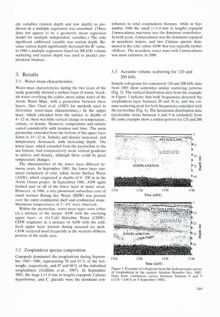
Sample echograms for concurrent 120 and 200 kHz data from 1985 show somewhat similar scattering patterns (Fig. 3). The vertical distribution data from the example in Figure 3 indicate that both frequencies detected the zooplankton layer between 20 and 30 m, and the vol- ume-scattering peak for both frequencies coincided with the pycnocline (Fig. 4). The horizontal-distribution data (pycnocline strata between 4 and 9 m excluded) from the same example show a similar pattern for 120 and 200

Time (ADT)

Figure 3. Example of echograms from the hydroacoustic survey of zooplankton in the eastern Alaskan Beaufort Sea, 1985. Data from continuous survey between Stations 8 and 9 (1116-1146 h on 8 September 1985).

'■mm

(a)l2Q kHz

Z O O P L A N K T O N ¥-31 g-' -, \ O

1

1126 1136

Tim e (ADT)

: r Y LINULLllNh kv 4

& L ̂ Z O O P L A N K T O N

349

Seawater Density ((g cm ^-1) 1000)1^.0 19.6 21.2 23.8 24.4 2Ç.0

Volume Scattering (V 2 m ̂ x lO * )

120 kHz

10 -200 kHzE

£

S' 20-Q

3 0 -

Figure 4. Examples of the vertical distribution of volume scat­tering (V2 m~3) during the continuous survey between Stations 8 and 9 (1116-1146 h on 8 September 1985). Sea-water density [(g cm ’-1)1000] is shown for Station 8.

kHz (Fig. 5). In both years, volume scattering was gen­erally much stronger for 200 kHz than for 120 kHz.

Data on the size distribution of the zooplankton ob­served during the survey are useful for interpreting the volume-scattering results from the 120 and 200 kHz systems. In 1985, the modal céphalothorax length for Calanus hyperboreus, the most abundant copepod, was 3.5 mm and for C. glacialis it was 2.5 mm. Given these sizes and the acoustic frequencies used during the study, the average backscattering cross-section was expected to be proportional to the fourth power of the frequency (the Rayleigh region, Greenlaw, 1979). The transition between Rayleigh and geometric scattering occurs when ka is about 1.0, where:

(2k ) (effective radius)ka = -------------- ;------ -------- .

wavelength

An effective radius is approximated by dividing animal length (cm) by 4. For 1985 and 1986 zooplankton data, the scattering was in the Rayleigh region (Table 2).

In 1985 at Station 3, the net sample at 8 m was 98 %

00 1.2tox)■E

200 kHz

>OJDC 0 . 6 -u

i °-4-COI 0 .2 -

i 4

^ 120 kHz

1116 1134 1140 11461112 1128

Time (ADT)

Figure 5. Example of the horizontal distribution of volume scattering (V: m ' ■’) during the continuous hydroacoustic sur­vey between Stations 8 and 9 (1116-1146 h on 8 September 1985). Pycnocline strata ( 4 - 6 and 6 - 9 m) are excluded.

copepods (mostly C. hyperboreus). Total sample bio­mass was 924 mg i t T 3 and density was 108 animals n T 3.

Volume scattering for 200 kHz was 2.4245 x 10~8, or —76 dB m-3 volume-scattering strength. Therefore, based on Pieper’s (1979) equation, the target-strength estimate is —96 dB/individual.

3.4. Zooplankton biomass regressions

3.4.1. 1985 regressionsThe relationship of net biomass per m3 vs. 200 kHz volume scattering was stronger than that for 120 kHz (Table 3). Given the Rayleigh scattering discussed in Section 3.2, this result was expected. The following geometric mean regression of zooplankton-net biomass per m 1 vs. 200 kHz volume scattering (Fig. 6) was ap­plied in the analyses of vertical and horizontal distribu­tions and patchiness in 1985:

Biomass (mg trT3) = 27.85 + (346.39)(VS x 10“).

3.4.2. 1986 regressionsThe 1986 volume-scattering data for 200 kHz, after thresholding out fish echoes, were regressed against zooplankton-net biomass. The 120 kHz data were not used in the 1986 biomass regression. The relationship

Table 2. Relationship between organism size and frequency for the copepods sampled with 120 and 200 kHz acoustic systems in the eastern Alaskan Beaufort Sea in 1985 and 1986 (ka defined in text).

Year Species Length (mm) ka 120 kHz ka 200 kHz

1985 Calanus h yp erb o reu s ....................................................... 3.5 0.458 0.7641985 Calanus g lacialis ................................................................ 2.5 0.330 0.5501986 Limnocalanus macrurus................................................... 1.5 0.196 0.327

350

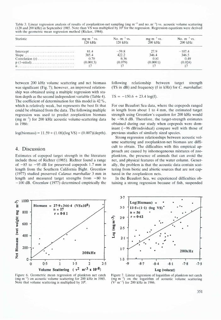
Table 3. Linear regression analysis of results of zooplankton-net sampling (mg i r r 3 and no. m '3) vs. acoustic volume scattering (120 and 200 kHz) in September 1985. Note than VS was multiplied by 10 for the regression. Regression equations were derived with the geometric mean regression method (Ricker, 1984).

Statistic mg m 3 vs. No. m 3 vs. mg m 3 vs. No. m 3 vs.120 kHz 120 kHz 200 kHz 200 kHz

In te rcep t ........................................................ 81.4 -5 9 .8 27.9 -107 .4S lo p e .............................................................. 385.4 422.2 346.4 346.5Correlation ( r ) ............................................. 0.70 0.36 0.81 0.49p (1-sided)............................................................ (0.0013) (0.079) (0.0001) (0.024)n ................................................................................. 17 17 17 17

between 200 kHz volume scattering and net biomass was significant (Fig. 7); however, an improved relation­ship was obtained using a multiple regression with sta­tion depth as the second independent variable (Table 4). The coefficient of determination for this model is 42 %, which is relatively weak, but represents the best fit that could be obtained from the data. The following multiple regression was used to predict zooplankton biomass (mg itT 3) for 200 kHz acoustic volume-scattering data in 1986:

log(biomass) = 11.59 + (1.08)(log VS) - (0.007)(depth).

4. Discussion

Estimates of copepod target strength in the literature include those of Richter (1985). Richter found a range of -8 5 to -9 5 dB for preserved copepods 1.7 mm in length from the Southern California Bight. Greenlaw (1977) studied preserved Calanus marshallae 3 mm in length and measured target strengths from —80 to -1 0 0 dB. Greenlaw (1977) determined empirically the

following relationship between target strength (TS in dB) and frequency (f in kHz) for C. marshallae:

TS = -150.6 + 23.4 log(f).

For our Beaufort Sea data, where the copepods ranged in length from about 1 to 4 mm, the estimated target strength using Greenlaw’s equation for 200 kHz would be —96.8 dB. Therefore, the target-strength estimates obtained during our study when copepods were dom­inant (—96 dB/individual) compare well with those of previous studies of similarly sized species.

Strong regression relationships between acoustic vol­ume scattering and zooplankton-net biomass are diffi­cult to obtain. The difficulties with this empirical ap­proach are caused by inhomogeneous mixtures of zoo­plankton, the presence of animals that can avoid the net, and physical features of the water column. Gener­ally, the problem is that the acoustic data contain scat­tering from biotic and abiotic sources that are not cap­tured in the zooplankton nets.

In the Beaufort Sea, we experienced difficulties ob­taining a strong regression because of fish, suspended

Biomass = 27-9+346-4 ( V S x l O ^ )

n = 17 r = 0-8 1

200kHz

Volume Scattering ( v2 m‘3 x 10'^)

Figure 6. Geometric mean regression of plankton net catch (mg m 3) on acoustic volume scattering for 200 kHz in 1985. Note that volume scattering is multiplied by 10®.

3-7

Log(Biomass) =

l l -5 + ( M ) (log VS) n = 56 r = 0-62

3-3

2-9

2-5

21

1-7200kHz

1-3

9 -8-7 -7-8-8 -4 •81 -7-5

Log (volscat)

Figure 7. Linear regression of logarithm of plankton net catch (mg i r r 3) on the logarithm of acoustic volume scattering (V m-3) for 200 kHz in 1986.

351

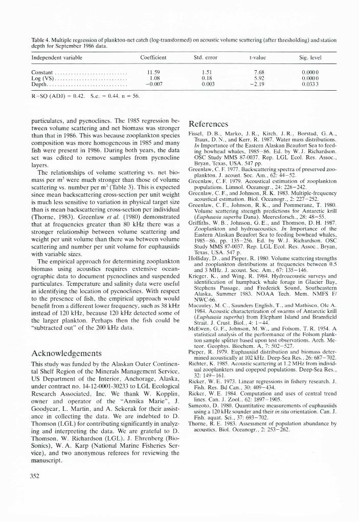
Table 4. Multiple regression of plankton-net catch (log-transformed) on acoustic volume scattering (after thresholding) and station depth for September 1986 data.

Independent variable Coefficient Std. error t-value Sig. level

C o n s ta n t ........................................... ........... 11.59 1.51 7.68 0.0000Log (V S )........................................... ........... 1.08 0.18 5.92 0.0000D ep th .................................................. -0 .007 0.003 -2 .1 9 0.0333

R - S Q (ADJ) = 0.42. S.e. = 0.44. n = 56.

particulates, and pycnoclines. The 1985 regression be­tween volume scattering and net biomass was stronger than that in 1986. This was because zooplankton species composition was more homogeneous in 1985 and many fish were present in 1986. During both years, the data set was edited to remove samples from pycnocline layers.

The relationships of volume scattering vs. net bio­mass per m3 were much stronger than those of volume scattering vs. number per m3 (Table 3). This is expected since mean backscattering cross-section per unit weight is much less sensitive to variation in physical target size than is mean backscattering cross-section per individual (Thorne, 1983). Greenlaw et al. (1980) demonstrated that at frequencies greater than 80 kHz there was a stronger relationship between volume scattering and weight per unit volume than there was between volume scattering and number per unit volume for euphausiids with variable sizes.

The empirical approach for determining zooplankton biomass using acoustics requires extensive ocean­ographic data to document pycnoclines and suspended particulates. Temperature and salinity data were useful in identifying the location of pycnoclines. With respect to the presence of fish, the empirical approach would benefit from a different lower frequency, such as 38 kHz instead of 120 kHz, because 120 kHz detected some of the larger plankton. Perhaps then the fish could be “subtracted out” of the 200 kHz data.

AcknowledgementsThis study was funded by the Alaskan Outer Continen­tal Shelf Region of the Minerals Management Service, US Department of the Interior, Anchorage, Alaska, under contract no. 14-12-0001-30233 to LGL Ecological Research Associated, Inc. We thank W. Kopplin, owner and operator of the “Annika Marie” , J. Goodyear, L. Martin, and A. Sekerak for their assist­ance in collecting the data. We are indebted to D. Thomson (LGL) for contributing significantly in analyz­ing and interpreting the data. We are grateful to D. Thomson, W. Richardson (LGL), J. Ehrenberg (Bio- Sonics), W. A. Karp (National Marine Fisheries Ser­vice), and two anonymous referees for reviewing the manuscript.

ReferencesFissel, D .B ., Marko, J R.. Kirch, J. R., Borstad, G. A.,

Traux, D. N., and Kerr, R. 1987. Water mass distributions. In Importance of the Eastern Alaskan Beaufort Sea to feed­ing bowhead whales, 1985-86. Ed. by W .J. Richardson. OSC Study MMS 87-0037. Rep. LGL Ecol. Res. Assoc., Bryan, Texas, USA. 547 pp.

Greenlaw. C. F. 1977. Backscattering spectra of preserved zoo­plankton. J. acoust. Soc. Am ., 62: 4 4 -52 .

Greenlaw, C. F. 1979. Acoustical estimation of zooplankton populations. Limnol. Oceanogr., 24: 226—242.

Greenlaw, C. F., and Johnson, R. K. 1983. Multiple-frequency acoustical estimation. Biol. Oceanogr., 2: 227-252.

Greenlaw, C .F ., Johnson, R. K., and Pommeranz, T. 1980. Volume scattering strength predictions for Antarctic krill (Euphausia superba Dana). Meeresforsch., 28: 48—55.

Griffiths, W. B., Johnson, G .E . , and Thomson, D .H . 1987. Zooplankton and hydroacoustics. In Importance of the Eastern Alaskan Beaufort Sea to feeding bowhead whales, 1985-86, pp. 135 - 256. Ed. by W .J. Richardson. OSC Study MMS 87-0037. Rep. LGL Ecol. Res. Assoc.. Bryan, Texas, USA. 547 p.

Holliday, D., and Pieper, R. 1980. Volume scattering strengths and zooplankton distributions at frequencies between 0.5 and 3 MHz. J. acoust. Soc. A m ., 67: 135-146.

Krieger, K., and Wing, R. 1984. Hydroacoustic surveys and identification of humpback whale forage in Glacier Bay, Stephens Passage, and Frederick Sound, Southeastern Alaska, Summer 1983. N O A A Tech. Mem. NMFS FI NWC-66.

Macauley, M. C.. Saunders English, T ., and Mathisen, Ole A. 1984. Acoustic characterization of swarms of Antarctic krill (Euphausia superba) from Elephant Island and Bransfield Strait. J. Crust. Biol., 4: 1-44 .

McEwen, G. F., Johnson, M. W., and Folsom, T. R. 1954. A statistical analysis of the performance of the Folsom plank­ton sample splitter based upon test observations. Arch. Me­teor. Geophys. Biochem. A, 7: 502-527.

Pieper, R. 1979. Euphausiid distribution and biomass deter­mined acoustically at 102 kHz. Deep-Sea Res., 26: 687-702.

Richter, K. 1985. Acoustic scattering at 1.2 MHz from individ­ual zooplankters and copepod populations. Deep-Sea Res., 32: 149-161.

Ricker, W. E. 1973. Linear regressions in fishery research. J. Fish. Res. Bd Can., 30: 409-434.

Ricker, W. E. 1984. Computation and uses of central trend lines. Can. J. Z oo l. ,62 : 1897-1905.

Sameoto, D. 1980. Quantitative measurements of euphausiids using a 120 kHz sounder and their in situ orientation. Can. J. Fish, aquat. Sei., 37: 693—702.

Thorne, R. E. 1983. Assessment of population abundance by acoustics. Biol. Oceanogr., 2: 253-262.

352