Patrizia

HYDROACOUSTICS AND UNDERWATER ACOUSTICS

New Virtual Sonar and Wireless Sensor System Concepts

J. A. Bucaro, B. H. Houston, and A. J. RomanoNaval Research Laboratory, Washington, D.C. 20375

Recently, exciting new sensor array concepts have been proposed which, if realized, could revolutionize how we approachsurface mounted acoustic sensor systems for underwater vehicles. Two such schemes are discussed here — so-called "virtualsonar" which is formulated around Helmholtz integral processing and "wireless" systems which transfer sensor informationthrough radiated rf signals. The "virtual sonar" concept provides an interesting framework through which to combat thedeleterious effects of the structure on surface mounted sensor systems including structure-borne vibration and variations instructure-backing impedance. The "wireless" concept would eliminate the necessity of a complex wiring or fiber-optic externalnetwork while minimizing vehicle penetrations.

INTRODUCTION

The growing possibility of being able to implementacoustic systems with high sensor counts (∼ 104) hasmotivated consideration of how we might exploitsuch a capability when it does indeed become areality. In particular, fiber optic sensor arraysutilizing in-fiber Bragg gratings and the revolutionunderway in MEMS/NEMS silicon-based sensortechnologies suggest that such high sensor countsystems might be “just around the corner.” Ourconsiderations of how one might exploit this futuretechnology for underwater vehicle sonars hascentered on long-standing technical and engineeringissues which have hampered these applications.These are, first and foremost, the deleterious effectsof structure-borne noise and hull impedance spatialand temporal variability. But they include as welllimited apertures and the necessity for multiple hullpenetrations for sensor signal feed through. Two newsensor array concepts — one called “virtual sonar”[1]and the other involving wireless arrays based oncellular communication[2] — offer a new perspectiveon how to approach surface mounted acoustic sensorsystems in the attempt to mitigate these problems.The "virtual sonar" concept provides an interestingframework through which to combat unwantedeffects of the structure on surface mounted sensorsystems. The "wireless" concept would eliminate thenecessity of a complex wiring external network whileminimizing vehicle penetrations. In the following, wediscuss these concepts and how they might besynergistically applied in the case of an underwaterAUV.

ARRAY CONCEPTS

Virtual Sonar

The “virtual sonar” concept[1] is based on simpleconsiderations of evaluating the Helmholtz integral

FIGURE 1. Helmholtz integral reconstruction for anincident plane wave, point force, and the two combined.

over the surface of an underwater structure for whichthere is high spatial density acoustic pressure andnormal velocity sensor data. The important resulthere is that for the case of a structure excited by bothan incident acoustic signal and interior noise sourcesapplied to the hull, when the acoustic field isevaluated inside the surface of the structure, only the“virtual” incident field remains. This is illustrated inFigure 1 taken from Reference[1] for an evacuated,thin cylindrical shell at kaa = 5, where ka is theacoustic wavenumber and a is the shell radius. Toillustrate the structural noise reducing properties of“virtual” sonar processing, Figure 2 displays thespatial Fourier transform of the pressure over thelength of the cylindrical shell section for this case.The lowest curve is the transform of the virtual sonarevaluated along the central axis, as well as for thetrue 1 Pa incident field (these two curves overlap).The upper curves are the transforms of the totalsurface response along a line on the lateral surface ofthe cylinder when the interior force (normalized bythe square of the shell thickness) is 104 Nt/m2 and 103

Nt/m2, respectively. One can see the superiorperformance of the virtual interior sonar regarding

structure-borne noise across the entire wavenumberspectrum including the acoustic domain (-ka to + ka).

0.1

1

10

100

1000

10000

-20 -15 -10 -5 0 5 10 15 20

104 Nt/m2

103 Nt/m2Exterior Line Array

Virtual Sonar

ka-ka

Wavenumber

FIGURE 2. Spatial Fourier transforms of the pressure overan exterior line and for the interior “virtual” line. Theexcitation is an incident plane wave and an interior pointforce. The transform for the incident field overlaps that forthe virtual sonar.

Results of the type shown above require sensorspatial sampling on the order of two per structuralwavelength. Azimuthally, the number of sensors, N,would be 2nmax, i.e twice the highest flexuralcircumferential harmonic. Axially, N would be2L/λf, i.e. twice the number of flexural wavelengths(λf) along the shell of length L. Now nmax ∝ (k aa)2/5

and λf ∝ (ka a)1/2. Calculations for the flexural wavedispersion and cut-off frequencies versus nmaxfor aplastic-like, 1.8m AUV shell structure predict thefollowing. At kaa = 1, about 103 measurement pointswould be required, while for kaa =10, about 8600.This requires indeed a large number of sensors;however, it would enable a “noiseless” array. Inaddition, with both pressure and velocity(acceleration) sensors employed, hull impedancespatial and temporal variations would be of noconsequence.

Wireless Array

One approach for accessing such a large sensorcount system is a wireless array. As depicted inFigure 3, wireless sensor/radios would be distributedover the surface of the structure. As many as onethousand sensor/radio pairs could be tied in to aspecific cell cite, and there could be tens of cells overthe body. The sensor information from this relativelysmall number of cells could be fed onto a single linewhich then penetrates the hull. The two majortechnology issues here involve propagation of theradiating gigahertz rf signals from sensors to basecell and powering of the individual sensor/radiodevices.

FIGURE 3. Wireless array on an AUV

In the case of a small AUV, an individual cellmight access sensors located within approximately ahalf meter radius. At the high rf frequenciesinvolved, the high absorption in water necessitatesthe introduction of a suitable waveguide material toallow sufficient propagation even over these modestbase-cell distances. The field strength of the lowestTEM order mode is approximately proportional to thefollowing factors

G ∼ c/ 2 / 0 π 2f r e − f r tan (1)

where c is the speed of light, is the dielectricconstant, f the frequency, r the propagation distance,

the permeability, and the loss factor. Eq. (1)indicates that what is desired is a material with a lowindex of refraction and a low loss factor. In water,the rf signal decays by 10-5 in 1 cm. This comparesto 2m, 12m, 20m, and 1km for polyurethane, nylon,Teflon, and Styrofoam, respectively. Thus, a thinlayer of a material of this type would provide asufficiently low loss waveguide in which topropagate the sensor-to-base cell signals. Estimates indicate that on the order of 1.5mW ofelectrical power would have to be supplied to eachsensor/radio pair assuming 10nJ/bit. This could bedistributed in a number of ways including powerbroadcasting and energy harvesting of thermalgradients or fluid flow.

ACKNOWLEDGEMENT

This work is supported in part by ONR.

REFERENCES

1. A.J. Romano, J.A. Bucaro, B.H. Houston, andE. G. Williams, J.Acoust. Soc. Am. 108, 2823-2828(2000)2. A. Mehrotra, Cellular Radio: Analog and DigitalSystems, Artech House, Boston, MA, 1994

Development of Thin, Low Frequency ElectroacousticProjectors for Underwater Applications

T. R. Howartha and J. F. Tresslerb

aNAVSEA Division Newport, Newport, RI USAbNaval Research Laboratory, Washington, DC USA

Two acoustic transducer panels have been designed, fabricated and electroacoustically evaluated. These panels featured‘cymbal’ drivers sandwiched between a radiating cover plate and a tungsten backing plate. The acoustic output showsresonance frequencies of both transducer panels below 1 kHz.

INTRODUCTION

The two most common acoustic projector technologiesused on unmanned underwater vehicle (UUV)platforms are tonpilz transducers and piezocomposites.Both of these technologies, however, are typicallydesigned for use at frequencies above 10 kHz. A U.S.Navy designed ‘1-3’ piezocomposite 2.54 cm in heightwith a projector radiating face of 15.24 cm by 7.62 cmwas demonstrated to exhibit broadband characteristicsbetween 10 kHz and 100 kHz [1]. At its resonancefrequency of 100 kHz, the TVR was measured to be174 dB//�Pa/V @ 1 m. At 1 kHz, the TVR was lessthan 110 dB//�Pa/V @ 1 m.To generate high acoustic output at frequencies below10 kHz, free-flooded piezoelectric ceramic rings,electromagnetic drivers, and flextensional transducershave traditionally been used. However, due to theirlarge size and weight, these technologies are not easilyadaptable or convenient for use in UUV platforms.For the implementation of low frequency acousticsources on UUV platforms, advanced hardware isrequired. The U.S. Navy has designed, built andevaluated novel prototype underwater electroacousticprojectors that have a fundamental resonancefrequency below 1 kHz. The active component ofthese projectors is slightly less than 0.5 cm in heightand has a radiating face of 15.24 cm by 7.62 cm,making them ideal candidates for use in mobileplatforms and littoral environments.

THE CYMBAL DRIVER

The low frequency underwater acoustic transducersutilize miniature class V flextensional drivers [2],commonly known as ‘cymbals’, as the active elementsin the projector. Cymbals were developed at the

Materials Research Laboratory at Penn State in themid 1990’s and have been investigated for use in anumber of applications [3]. A cymbal consists of anelectroactive ceramic disk sandwiched between andmechanically bonded to two thin metal caps. Each capis shaped in a die press so that it will contain a shallowair cavity underneath its inner surface after it is bondedto the face of the ceramic disk. The caps serve asmechanical transformers for converting the smallradial displacement and vibration velocity of theelectroactive disk into a much larger axial directiondisplacement and vibration velocity normal to the apexof the caps. Hence, the cymbal driver primarilyutilizes the ‘31’ contribution of the active ceramic toachieve flexure in the caps.Cymbals with two different diameters (12.7-mm and15.9-mm, designated as Type 1 and Type 2,respectively) were used in this study. Titanium wasselected as the cap material because of its low density(4500 kg/m3), moderate elastic modulus (120 GPa),and oxidation resistance. The electroactive materialwas Navy Type VI (PZT-5H) piezoelectric ceramic.This material was selected because its very largepiezoelectric d31 coefficient served to generate thelargest flexure (i.e., displacement) in the caps.Prior to bonding the caps to the ceramic, studs 1.4 mmin diameter and 4.6 mm long with UNF 0-80 threadswere welded to the apex of the caps to form both themechanical and electrical means of handling.

ACOUSTIC TRANSDUCTION PANEL

The low frequency acoustic projector panels consistedof an array of cymbal drivers sandwiched between a12.7 mm thick tungsten backing plate and a 2.2 mmthick copper electroplated carbon graphite epoxy board(solid all uni-carbon from Aerospace Composite

Products, San Leandro, CA). Figure 1 shows thecymbal elements mounted into the tungsten backingplate before the cover plate was attached.

FIGURE 1: Cymbal elements on backing plate.

The total radiating area of the projector was 152.4 mmby 76.2 mm. Two transducers, designated as Xducer Iand Xducer II, were built and tested. Xducer Iconsisted of 50 Type 1 cymbal drivers in a 10 by 5arrangement. Xducer II contained 32 Type 2 elementsin an 8 by 4 configuration. The studded cymbals wereinitially torqued into a predrilled and threaded tungstenbacking plate. Next, the drilled out graphite coverplate was lowered into place so that it rested over thetop of the cymbal array. The cover plate was similarlytorqued onto the studded cymbals with hex nuts.Standard underwater calibration measurements on thelow frequency projectors were performed at theNAVSEA Division Crane Glendora Lake Facility inSullivan, Indiana. The measurements were performedat a depth of 11.3 meters and a water temperature of 10degrees C. The transmitting voltage response (TVR)for the transducers as a function of frequency wasmeasured from 0.5 kHz to 100 kHz and is shown infigure 2. The low frequency resonances, 0.6 kHz inthe case of Xducer II and 0.9 kHz in the case ofXducer I are a result of the piston-like motion of thecover plate being driven by the individual cymbaldrivers. Both projectors exhibit markedly higher TVRthan that of a 1-3 piezocomposite with the sameradiating area. Unlike the 1-3 piezocomposite,however, the cymbal-based transducers aremultiresonant as the cap and flexing graphite platesflex throughout the frequency bands. The beampatterns at 1 kHz for the two projectors both show theomnidirectional response as is to be expected at thesefrequencies. The sound pressure level (SPL) wasmeasured for Xducer I as a function of frequency anddrive level. Nonlinear behavior becomes apparent at adrive level above 500 Vrms. The transducer was only

driven to a maximum of 750 Vrms because furtherevaluation was desired and we didn’t want to take therisk of failure. Comparing the transmitting response ofXducer I both before and after being subject to a drivelevel of 750 Vrms indicated no adverse effects due tothe high drive.

100

110

120

130

140

150

0.1 1 10 100

TV

R (d

B//u

Pa/V

@ 1

m)

Frequency (kHz)

12.7-mm diameter driver (solid line)15.9-mm diameter driver (dashed line)

FIGURE 2: TVR comparison of transducers.

ACKNOWLEDGMENTS

The authors express their appreciation to WalterCarney, Kirk Robinson and Mel Jackaway ofNAVSEA Crane Division for fabrication andmeasurements of the panels. The authors acknowledgethe support of the Office of Naval Research.

REFERENCES

1. T.R. Howarth and R. Y. Ting, “Development Of ABroadband Underwater Sound Projector,” CDProceedings of OCEANS ‘97 MTS/IEEE Conference,IEEE Publications (ISBN 0-7803-4111-2/97),Piscataway, NJ, 1-7, 1997.

2. R. E. Newnham and A. Dogan, Metal-electroactiveceramic composite transducer, U. S. Patent 5,729,077,issued March 17, 1998..

3. J. Zang, W. J. Hughes, P. Bouchilloux, R. J. Meyer Jr., K.Uchino and R. E. Newnham, "A Class V flextensionaltransducer: The Cymbal," Ultrasonics, 37, 387-393,1999.

Experimental Results of Passive Phase Conjugation Applied toUnderwater Acoustic Communication

W. L. J.Fox, D. Rouseff, D. R. Jackson,andC. D. Jones

University of Washington, Applied Physics Laboratory, 1013 NE 40th St., Seattle, WA 98105, USA

In May 2000, an experimentwas performedto demonstratethe effectivenessof passive phaseconjugation(PPC)for underwateracousticcommunications.PPCis a coherentarray and signal processingschemethat hasstrongtheoreticalties to active phaseconjugationandtime-reversalmirrorsin theocean.It differsfrom active techniquesin thatanarrayof transducersneedonly receive,while thetransmittercanbea singletransducer. Previousresultshave beenpresentedshowing performanceof thealgorithmfor caseswith averticalreceive arrayspanningthewatercolumn.Thispaperwill show furtherresultswith a truncatedreceive array.

THEORETICAL FOUNDATIONS OFPASSIVE PHASE CONJUGATION

Phase conjugate acoustics have previously beendemonstratedin the ocean[1]. The basicphenomenoncan be describedby the following. A sourcetransmitsa signal,a distortedversionof which is received by thetransducerssof adistantverticalarray. Thesignalis typi-cally distortedby timespreaddueto multiple interactionswith theseasurfaceandbottomasit propagatesdown theacousticchannel. If thesedistortedreceive signalsaretimereversedandtransmittedfrom their respectivetrans-ducers,it canbeshown theoretically[2] thattherewill bea spatio-temporalfocusingof this secondtransmissionatthelocationof theoriginal transmission.

It is the time-spreaddistortionmentionedabove andits timevariablenaturethatposethemainhurdlesto highdatarateunderwateracousticcommunications.Compu-tationally complex adaptive equalizersare the standardtechniquefor addressingtheseproblems. A techniquecalledpassive phase conjugation (PPC)hasbeendevel-opedandpresented[3, 4] asacomputationallysimpleal-ternative.

PPCis designedfor coherentlymodulatedcommuni-cationfrom a point in thewatercolumnto anarraywithvertical spatial diversity. In its most simple form, thecommunicatingsourcesendsaprobesignalfollowedby ablankingperiodto allow for channelclearingfollowedbythecommunicationsymbolstream.Thereceiversinitallyseethe probesignal followed by the time-spreadmulti-paths.Eachchannelusesthis estimatedchannelimpulseresponse(differentfor eachreceiver) asa matchedfilterfor thefollowingcommunicationssymbols.Theresultingmatchedfilter outputsareintegratedover the array. Fora vertical array that spansthe watercolumnwith denseenoughspatialsampling,theresultcanbeshown to can-cel nearly perfectly inter-symbol interference[4], anal-ogousto the theoreticalfoundationsof the active phaseconjugationphenomenon.Timevariabilityof thechannel

impulseresponsescanbemeasuredby re-probing,whichdoesimposeacertaindatarateoverhead.

EXPERIMENTAL RESULTS

An experiment to demonstratethe effectivenessofPPC for underwater acousticcommunicationwas per-formed in PugetSoundnearSeattle,WA in May 2000.Some resultsof that experimentwere previously pre-sented[3, 4]. Thoseresultswerefor caseswherethe re-ceive array spannednearly the entire water column. Asimilar caseis shown in the first examplehere. For thispartof theexperiment,bothvessels(sourceandreceiverdeployment)were mooredin � 30 m of water roughly650m awayfrom eachother. Thesourcewasdeployedata depthof � 15 m.

Figure1 showsthechannelimpulseresponsesasmea-suredon the 14-elementreceiving array, with elementspacingof � 1 � 7 m. This configurationspannedroughly74%of thewatercolumn. Theprobewassent,followedby a 50 ms blank window to measurethe channelim-pulseresponse,subsequentlyfollowedby the communi-cationssymbolstreamwhichcanbeseenat theright sideof Fig.1. TheaverageestimatedSNRperchannelfor thiscaseis 12.9dB usingtheequation

SNRest� 14

∑n � 1

�N50

∑i � 1

xi � n2 � N50

∑j � 1

x j � n2 �14∑

n � 1

�N50

∑j � 1

x j � n2 � � (1)

whereN50 is thenumberof datasamplesin a 50 mswin-dow, the indices i correspondto samplesafter the startof the probereception,the indices j correspondto sam-plesbeforetheprobereception(i.e., noiseonly), andthex i � j �� n arethereal-valueddatasamplesfrom receivern.

The datawere transmittedas a random(but known)sequenceof binaryphaseshift keyed(BPSK)symbolsat

1.04 1.05 1.06 1.07 1.08 1.09

14

13

12

11

10

9

8

7

6

5

4

3

2

1

Time (s)

Rec

eivi

ng H

ydro

phon

e

Raw Hydrophone Data: 130145916

FIGURE 1. Probepulse responseon 14-elementarray withstartof datasequence,elementspacing� 1 7 m.

0 1 2 3 4 5−1.5

−1

−0.5

0

0.5

1

1.5

Time (s)

Con

stel

latio

n

Output of DBPSK Processing: 130145916

FIGURE 2. DifferentialBPSK demodulationresults,elementspacing� 1 7 m.

a rateof 2174symbolspersecond,anddemodulateddif-ferentially(i.e.,phaseshift betweensymbols,ratherthanabsolutephase,is important).Theresultof thedemodu-lation canbeseenin Fig. 2. Ideally, valuesdifferentiallyencodedas’1’ will takeonavalueof 1.0in theconstella-tion plot, andvaluesencodedas’0’ will takeonavalueof-1.0in theplot. The’x’ symbolsdenotesymbolsencodedas’1’, andthe ’o’ symbolsdenotethoseencodedas’0.’Notethatthereareno symbolerrorsin this dataset.

Roughly 100 minutes later, data was taken with are-deployed receive array whoseelementspacingwas� 1 � 0 m, i.e., spanningroughly 43% of the water col-umn. Figure 3 shows the demodulationresultsfor thiscase. At this time the noisebackgroundhad increased,with SNRest

� 2 � 2 dB.DespitethedecreasedSNRandre-ducedwatercolumncoverage,error-freecommunication

0 1 2 3 4 5−1.5

−1

−0.5

0

0.5

1

1.5

Time (s)

Con

stel

latio

n

Output of D−BPSK Demodulation: 130163949

FIGURE 3. DifferentialBPSK demodulationresults,elementspacing� 1 0 m.

wasstill achieved. Note,however, that theconstellationshave widenedandmoved closerto 0, meaninga higherprobabilityof symbolerror.

Futurework on this topic will include investigationof the algorithm’s performancefor non-vertical arrays.We will alsolook at thecomputationalandperformancetrade-offs involvedwith usingdecisiondirectedblockes-timationof thechannelimpulseresponsein placeof theisolatedprobeconcept.

ACKNOWLEDGMENTS

This work was funded by the Office of Naval Re-search.

REFERENCES

1. W. A. Kuperman,W. S.Hodgkiss,H. C. Song,T. Akal, C.Ferla,andD. R. Jackson,J.Acoust.Soc.Am., 103, pp.25-40.

2. D. R. JacksonandD. R. Dowling, J.Acoust.Soc.Am., 89,pp.171-81.

3. D. R. Jackson,D. Rouseff, W. L. J. Fox, C. D. Jones,J.A. Ritcey, andD. R. Dowling, J. Acoust.Soc.Am., 108,p. 2607.

4. D. R. Jackson,D. Rouseff, W. L. J.Fox, C. D. Jones,J.A.Ritcey, andD. R. Dowling, "Underwateracousticcommu-nicationby passive phaseconjugation:Theoryandexperi-mentalresults,"IEEE J. OceanicEng.(acceptedfor publi-cation).

Optimal Superimposing of the Normalized Quasi RigidEcho Spectrum on the Quasi Rigid Form Function :

Targets Sizing

P. Schweitzera, J. Mathieua,b, E. Tisseranda, D. Bellefleurb

aL.I.E.N., Faculté des Sciences, Université Henri Poincaré - NANCY I, B.P. 239, 54506 VANDOEUVRE-LES-NANCY CEDEX, FRANCE. bG.E.M.C.E.A. - 149, rue Gabriel Péri - 54500 VANDOEUVRE-LES-NANCY

We developped a methodology based on the analysis of the backscattered echo from an immersed target for thedetermination of its size. The Quasi Rigid Backscattered Echo (QRBE) defined as the first part of the backscattered echocontains the size information of the target. The Quasi Rigid Form Function (QRFF) is then constructed by consideringonly the quasi rigid backscattered echo. The Normalized QRBE spectrum obtained by practice can be interpreted as asegment of the QRFF. The object of this paper is to present how we find the optimal super imposition between them inorder to find the size of the target. We present successively the two steps for the method. First we determine the classes ofsolutions according to the system bandwith B in use. These classes are defined by all the size for which the QRFF has thesame and type of extrema. We improve then this estimate by mean squares criterian applied in this class of belonging. Wepresent the experimental setup and show different size determination results for different steel wires.

INTRODUCTION

We propose an ultrasonic method to determine thesize of an immersed wire. This can be done comparingits quasi rigid backscattered echo spectrum on areference function. The different steps of the methodof surimposition in order to find the size of the targetare presented successively in this paper.

THE QUASI RIGID BACKSCATTEREDECHO (QRBE)

We define the QRBE, for an immersed target(wire) in water and insonified by a plane ultrasonicwave, as the first part of the backscattered echo. Itsduration is equal to the backscattered echo of aninfinitively rigid wire of same size.

The first part of the echo is mainly constituted byScholte-Stoneley and specular waves which containthe size information of the target [1].

THE QUASI RIGID FORM FUNCTION(QRFF)

Contrary to the form function which expresses allthe scattering waves generated by a wire, there is noanalytical expression of the QRFF fQR(ka). The quasirigid form function is calculated by taking into accountthe quasi rigid part of the echo we simulate. Thedetails of the method is given in [2].

FIGURE 1. Modulus of the steel QRFF versus ka.

EXPERIMENTAL CONDITIONS

The samples (steel wires) are vertically imbeddedin a tank filled with still water. The emitter-receiver isa broadband transducer of 1 cm diameter, acting infrequencies in the range of 0,7 MHz to 1,5 MHz.

SIZING BY SPECTRAL ANALYSIS.

Method

The first step of our method is the calibration.

We calculate the spectrum )f(EblockQR of the QRBE from

a block which simulate a solid half space. Then thisblock is replaced by the wire to be sized

The ratio )f(E

)f(E )f(E

blockQR

wireQR

NQR � can be interpreted as

a segment of the quasi-rigid form function.

0 1 2 3 4

0.81

11

ka

Relative amplitude

)f(EwireQR is the quasi-rigid part of the echo.

This relation is only valid in the limited bandwidthB of the measuring chain so for ka limited to the

interval ��

���

����� ac

f2 ; acf2 maxmin . c is the sound speed

in water and “a” the size of the targetThe last step is to determine the size of the wire

under test by replacing the segment )f(ENQR on theQRFF.

Positioning the segment on the QRFF

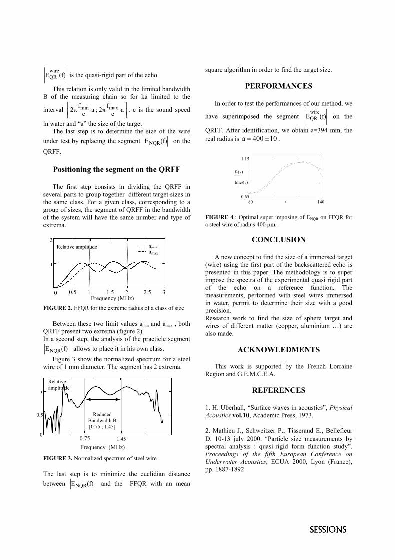
The first step consists in dividing the QRFF inseveral parts to group together different target sizes inthe same class. For a given class, corresponding to agroup of sizes, the segment of QRFF in the bandwidthof the system will have the same number and type ofextrema.

FIGURE 2. FFQR for the extreme radius of a class of size

Between these two limit values amin and amax , bothQRFF present two extrema (figure 2).In a second step, the analysis of the practicle segment

)f(ENQR allows to place it in his own class.Figure 3 show the normalized spectrum for a steel

wire of 1 mm diameter. The segment has 2 extrema.

FIGURE 3. Normalized spectrum of steel wire

The last step is to minimize the euclidian distancebetween )f(ENQR and the FFQR with an mean

square algorithm in order to find the target size.

PERFORMANCES

In order to test the performances of our method, we

have superimposed the segment )f(EwireQR on the

QRFF. After identification, we obtain a=394 mm, thereal radius is 10 400 a �� .

1.15

0.65

f�( )�

fmes( )�

14080 �

FIGURE 4 : Optimal super imposing of ENQR on FFQR fora steel wire of radius 400 �m.

CONCLUSION

A new concept to find the size of a immersed target(wire) using the first part of the backscattered echo ispresented in this paper. The methodology is to superimpose the spectra of the experimental quasi rigid partof the echo on a reference function. Themeasurements, performed with steel wires immersedin water, permit to determine their size with a goodprecision.Research work to find the size of sphere target andwires of different matter (copper, aluminium …) arealso made.

ACKNOWLEDMENTS

This work is supported by the French LorraineRegion and G.E.M.C.E.A.

REFERENCES

1. H. Uberhall, “Surface waves in acoustics”, PhysicalAcoustics vol.10, Academic Press, 1973.

2. Mathieu J., Schweitzer P., Tisserand E., BellefleurD. 10-13 july 2000. �Particle size measurements byspectral analysis : quasi-rigid form function study”.Proceedings of the fifth European Conference onUnderwater Acoustics, ECUA 2000, Lyon (France),pp. 1887-1892.

Frequency (MHz)1.450.750

0.5

1

ReducedBandwidth B[0.75 ; 1.45]

Relativeamplitude

0 0.5 1 1.5 2 2.5 3

1

2

Frequency (MHz)

aminamax

Relative amplitude

Implosion Sound SourcesN. Yen

CLY Associates, P. O. Box 6806, Alexandria, VA, 22306-6806 USA

Acoustic pressure caused by implosion has impulsive characteristics similar to those generated by an explosive, but the signature ishighly temporally and spatially localized without the safety issues with explosives. The present study focuses on the practical utilizationof a highly concentrated pressure pulse caused by an implosion mechanism as a sound source. The operational principle of an implosionsound is simply derived from the conversion of hydrodynamic energy to acoustic energy from the collapse of a cavity. However, thecontrollability of an implosion can be manipulated by directing the one-dimensional flow into a confined specially shaped cavity to formthe spherical convergence. Based on the physics of the collapse of a spherical cavity, the reflection of a self-focused wave can create adelta-function like pressure pulse. For underwater application, because no air is trapped in the closed space initially, the acousticsignature is a simple pressure pulse without any interference of bubbles generally observed in the explosive or air gun operations. Thesimple structure of the implosion mechanism can be adapted for various engineering designs to meet the practical needs inoceanographic and underwater research activities.

INTRODUCTION

Current technology for generating impulsive sound wavesfor underwater surveying and communication applicationsemploys the detonation mechanism. The acoustic signalobtained in this way is not controllable: it consists ofinterference caused by bubbles' resonances and it issensitive to the variation of charges and operational depth.Other methods use various types of frequency synthesisapproaches to form a broad band signal. However, such asound source is not temporally and spatially localized, andits efficiency is low due to the compensation of frequencyresponse during the electro-mechanical transduction. Ahighly concentrated pressure pulse caused by an implosionmechanism appears to alleviate those problems. A briefreview on some of the implosion underwater sound sourcesis given in references 1. The presentation covered in thisshort paper is focused on the control of the implosion soundgeneration. Extensive discussion of this subject is describedin references 2 and 3.

IMPLOSION MECHANISM

Implosion is formed by directing waves toward a focalcenter. Because of the energy concentration, an extremelystrong pressure and high temperature can be built up in avery small region, thereby generating a sharp shock wavepropagating outwards. A simple mathematical model of thisphenomenon can beformulated by the collapse of a spherical void such as theRayleigh-Plesset's equation used in analyzing thecavitation. The phenomenological interpretation of theimplosion process sequence shown in Fig. 1 are: (a) thecollapse of a bubble generates a spherical shock wave, (b)the implosion shock wave converges to the cavity center,(c) a high pressure pulse is created by energy concentration,(d) the intensity of a shock front is enhanced by reflection,

(e) tremendous temperature at the center causesdissociation, (f) light emits from black body radiation orionization, (g) the reflected implosion propagates out as asound pulse. The acoustic emission from a 65 �m bubblemeasured in the laboratory [4] has an intensity magnitudeabout 170 dB/1�Pcal. The estimated conversionefficiency from the mechanical energy to the acousticenergy is about 75%.

(a) (b) (c) (d) (e) (f) (g)

FIGURE 1. Phenomenological Interpretation of Implosion

CONTROLLED IMPLOSION

The practical way to generate a controlled implosion isthrough the manipulation of a plane shock wave [5]according to the Chester-Chisnell-Whitam (CCW) model[6] by forcing it to converge to a single point. Fig. 2(a)shows closed tubes with three different shaped terminals:(i) cylindrical, (ii) CCW form, (iii) conical. The measuredwaveforms of implosion sound from those controlledenclosed cavities of one inch diameter tube are displayedin Fig. 2(b) respectively. The highest peak pressure pulsecan reach to an intensity of 190 dB/1�Pcal. The CCWshaped terminal provides a well defined pulse with aduration of less than 100 �s.

0 .15 .3 ms (a) (b)

FIGURE 2. Enclosed Cavity Implosion

IMPLOSION SOUND PROJECTORS

Various types of implosion sound projectors [3] can beconstructed based on the controllable implosion schemedescribed in the previous section. Their design parametersdepend on the application requirements and costconstraints. The sketch shown in Fig. 3 is a project elementwhich has the feature that can be integrated with underseasurvey system for directional scanning. This soundgenerated unit consists of a housing #61, the implosionchamber # 14 with its implosion center at #16. Anelectronic controlled valve #66 is used to create an artificialvoid in #14 with a vacuum pump. For the implosionoperation, the valve switches the tube connection to a high-pressure tank and forces the fluid #38 inside the housingsquash to the tip of the chamber #62 and causes aconvergent collapse center at # 16. The cover #57 is anacoustic transparent material so the generated acousticwave can be directed out through this window. Many ofsuch a unit #40 can be arranged to form an array. With theproper placement of implosion units and timing delayopening of control valves, a directional radiated sharpimplosion acoustic impulse can be formed. Preliminarytests of a chamber size of 1" diameter and 1.5" in depth inthe laboratory tank operated with vacuum of 0.022 ATMand a high-pressure of 1 ATM, generates an impulse ofpeak intensity 195 dB/1�Pcal with a pulse width less than50 �s at 3 feet away from the implosion projector can bedirected to a desired direction for remote scanning search.

FIGURE 3. An Implosion Sound Projector

DISCUSSION

The use of an implosion sound source described herehas demonstrated that an underwater acoustic wavegenerator designed with this type of mechanism is simpleand safe to operate for undersea remote surveyingapplication. At the current stage, only a simple prototypehas been constructed and laboratory tests havedemonstrated its practicability for underwater applicationas an effective sound source. Because of the simplicity ofthe implosion mechanism in comparison with thetraditional acoustics radiators, this type of a sound sourcehas much better performance features in the areas ofacoustic signature (a temporal and spatial concentratedwide band signal), operation handling (light weight),system integration (small size), and low cost (less logisticsupport). Many alternative designs other than thosementioned in this paper can be adapted for someengineering modifications to meet the needs inoceanographic and underwater research activities. Futureeffort for implosion acoustics studies will be directed tothe optimization of the structure design based on aspecific task requirement.

REFERENCES1. Yen, N., "Application of Implosion to Underwater Sound

Generation”, J. Acoust. Soc. Am. 100, p 2716, (1996).

2. Yen, N., “An Implosion Sound Source for Undersea ExplorationApplications”, in Proceedings of Second International Ocean andAtmosphere Conference, Central Weather Bureau, Taipei, 2000,pp. 315-318.

3. Yen, N., An unpublished NRL proposal and "ControllableImplosive Sound Projector", Reg. Number H1664, United StatesStatutory Invention Registration, July 1, 1997.

4. Stottlemyer, T.R., An Experimental Study of the Acoustic Emissionfrom Collapsing Cavities in Liquids, A Ph. D. dissertation, YaleUniversity, New Haven, 1996.

5. Yen, N., "Controlled Implosion Sound Generation", NonlinearAcoustics in Prospective, 14th International Symposium onNonlinear Acoustics, Ed. R. J. Wei, Nanjing University Press,Nanjing, 1996, pp 292-297.

6. Whitham, G.B., Linear and Nonlinear Waves, Wiley-Interscience,New York, 1974

Surface Acoustic Waves for Sediment Characterization;from Sonar to Tomographic Approach

M. E. Zakharia a and E. Mouton b

a French Naval Academy IRENav, 29240, Brest Naval, France, zakharia@ecole-navale.frb SAGE-GEODIA, Les Clachs, 34560, Poussan, France, emo@sage-geodia.com

Surface acoustic waves (such as Stoneley-Scholte Waves (SSW) travel along the interface between the seawater and theseabed; they are guided in a layer of about a wavelength and carry information on the first meters of sediment. Their velocitycan be used for the inversion of fine properties of the sediment. Several experiments have shown that these waves can also beused for the detection of buried objects. Experiments on tomographic reconstruction of an anomaly in the sediment using SSW(impedance changes due to the presence of bubbles, for instance) have provided very interesting results and highlighted therelevance of such a technique for sediment description at sea.

INTRODUCTION

Several applications (such as offshore, cable andpipeline installation, mine detection, propagationprediction, slope stability studies…) need an accurateknowledge of the seabed properties. This work willshow how Stoneley-Scholte Waves (SSW) can be arelevant tool for seabed characterization and sub-bottom imaging.

Fine characterization of sediments

As the penetration depth of SSW depends on thefrequency, each frequency bin carries information on acorresponding layer; when using wideband signals, thegroup velocity dispersion of the SSW depends on thevelocity profile in the sediment. The group velocitycan be easily measured on a time-frequencyrepresentation of wideband transmitted signals [6].Several simulations and experiments have shown thatvelocity dispersion could be predicted with accuracybetter than 5% (direct problem) [6].

The inverse problem consists in determining thesediment properties from SSW properties. A newapproach, based on neural network has been developedfor this purpose. It showed, on experimental data, thata comparable accuracy (better than 5%) can beobtained on the data from inverse problem solution[5]. Such results were very encouraging: if SSWproperties are sensitive to small changes in thesediment, they should be very sensitive to the presenceof a buried target (large variation of impedance).

Detection of a buried object

Several tank experiments have been carried out onburied targets in a homogeneous resin [4]. For atransmitter position, the surface was finely scannedand the SSW energy on the interface was computed.Figure 1 displays the results of such a computation. Inthis figure, one can see from top to bottom:� the incoming wave loosing some energy while

propagating,� a zone of interference between the incoming wave

and the one reflected by the sphere� a shadow zone after the sphere very similar to

shadows encountered in sidescan sonar.

FIGURE 1. Energy distribution of SSW at waterbottom interface in the presence of a spherical target

size: 16 mm; frequency 0.1 MHz, wavelength 10 mm.2-dB/ gray level, scales 0.1 x 0.1 meters.

Similar effects have been observed for various targets(even when comparable in size to a wavelength). Theyshowed that the presence of a target scatters the energyof SSW in all direction (instead of forward direction).

The absence of energy can thus be used to detect thepresence of a target (like in sidescan sonar).Preliminary work (still in progress) has shown that asonar approach (monostatic transmitter and receiver)can also be used for target detection.

Reflection and transmission properties

The reflection and transmission of SSW was studied inthe solid-solid configuration. As they are evanescentwaves, two hypotheses have been found: continuityconditions for either each component or their resultant.From experiments, we have found that the second onematches better and that, at oblique incidence, SSWfollow laws similar to Snell-Descartes ones [2]:� SSW is reflected as a SSW (with same velocity)� SSW is transmitted as another SSW (with a SS

velocity corresponding to the second medium)� A critical angle was observed (similar to the one

encountered for compression waves).� No other waves or components were observed.

Tomography

The properties cited above allowed a tomographicreconstruction of velocity using SSW. Several mock-ups and geometrical configurations were studied usinga cylindrical inclusion in homogeneous sediment [3].Figure 2 shows an example of tomographicreconstruction of the SSW velocity. The position ofthe inclusion has also been displayed on the figure.The results clearly show the high quality oftomographic reconstruction using the backpropagationmethod.

CONCLUSION

Results from various tank experiments and associatedsignal processing schemes showed the ability of SSWto provide accurate information on fine characteristicsof the sediments and to be used for sub-bottomimaging and the detection of buried objects. Next stepis the application of the techniques described andvalidated in tank to the seabed and to real applications(in situ).

ACKNOWLEDGMENTS

The work was achieved in LASSSO laboratory(Laboratoire d’Acoustique, Systèmes, Signaux etSonar, at CPE, Lyon.) and was partly supported by theEuropean Commission and by the French MOD.

FIGURE 2. Tomographic reconstruction of acylindrical inclusion in a resin.

Scales: 0.2 x0.2 m, 18 m/s by gray level

REFERENCES

1. M. E. Zakharia and P. Chevret « Neural networkapproach for inverting velocity dispersion; applicationto sediment and to sonar target characterization, InverseProblems 16 (2000) 1963-1708.

2. E. Mouton, J. Châtillon et M.E. Zakharia, Etudeexpérimentale de la réflexion et de la transmission desondes de surface de type Stoneley-Scholte à l'interfacede deux milieux solides, Actes du 5e Congrès Françaisd'Acoustique, CFA 2000, septembre 2000, Lausanne,Suisse, pp. 80-83.

3. E. Mouton and M. E. Zakharia, Reconstruction ofsediment inhomogeneities using surface wavetomography, in Proceeding European Conference onUnderwater Acoustics (ECUA2000), Lyon, July 2000,M.E. Zakharia, P. Chevret and P. Dubail editors,European Commission Brussels (Belgium), Vol. 1 pp.245-250.

4. M.E. Zakharia and J. Châtillon, Interaction of interfacewaves with a buried object, in Proceedings of The ThirdEuropean Conference on Underwater Acoustics(ECUA), Heraklio (Greece), June 1996, J.S. PapadakisEd., European Commission Brussels, pp. 39-44.

5. J. Guilbot and M. Magand, Determination of thegeoacoustical parameters of a sedimentary layer fromsurface acoustic waves: a neural network approach,Conference on Full Field Inversion Methods in Oceanand Seismic Acoustics, O. Diachock, A. Caiti, P.Gerstoflt and H. Scmidt Eds, Kluwer AcademicPublishers, pp.171-176, 1995.

6. J. Guilbot and M.E. Zakharia, Tank experiments on asediment small-scale model. Shear wave velocityprofile inversion via Stoneley-Scholte waves, inProceedings of The Second European Conference onUnderwater Acoustics (ECUA), Lyngby (Denmark),July 1994, L. Bjørnø Ed., European Commission,vol. II, pp. 979-984.

Stationary hydroacoustic methodology to determine diel activity of fish biomass in the artificial habitats

Sala A.(1), Fabi G. (1)

(1) Istituto di Ricerche sulla Pesca Marittima (IRPEM), Consiglio Nazionale delle Ricerche

Largo Fiera della Pesca, 1 – 60125 Ancona, Italy The biomass of fish assemblage, inhabiting the Senigallia artificial reef (central Adriatic sea, Italy), was evaluated in the period July–November 1996. Density and biomass were assessed through a stationary hydroacoustic methodology using an appropriately adapted SIMRAD EY500 system. A part of the system was placed inside the reef and it was linked by radio-modem to the remaining part installed ashore in the Institute. The experimentation gave useful information about the daily behaviour of the fish assemblage living at the reef: during the whole period the lowest densities were generally recorded in the early afternoon, whilst the highest abundances were commonly observed late in the night and in the early morning. Acoustical records confirmed that in late summer–early autumn most of the reef fishes migrate from the coastal shallow waters to offshore. Throughout the study period the fish abundance was higher inside the reef and decreased significantly at a distance of about 80 m from the structures.

EXPERIMENTAL DESIGN An acoustic fixed technique was applied for the

valuation of the fish biomass at an artificial reef deployed along the coast of the central Adriatic sea (1.2 nmi offshore, 12 m depth).

The hydroacoustic equipment consisted of Simrad EY500 echo-sounder and comprised: - 1 transceiver with Personal Computer; - 4 batteries (charged with solar panels); - 1 transducer-multiplexing (SIMRAD MP500); - 1 timer, to periodically power the system.

All the above equipment, was placed inside a waterproof case on a fixed buoy inside the reef area.

The EY500 system was linked by a radio-modem to another Personal Computer installed ashore in the Institute, which through an appropriately developed program automatically controlled the correct functioning of the EY500 system in real time.

Four split-beam transducers (120 kHz) were settled to measure in situ fish Target Strength distribution and density: - transducer 1 (T1), placed 4m-deep on the fixed

buoy’s pile, was horizontally oriented towards the centre of the reef;

- transducers 2 and 3 (T2, T3) were located on steel frames placed on the bottom inside the artificial reef and upward-oriented;

- transducer 4 (T4) was oriented towards the surface, as T2 and T3, but located on the bottom outside the artificial reef, about 80 m far. Every two hours the system was powered on by the

timer for a period of 16 minutes and the echo-sounder started pinging immediately.

The equipment operated continuously and the acoustic data, received from the echo-sounder, were stored on the computer’s hard-disk in a telegram-based structure. Contemporarily, every 60 seconds, the system transferred through the radio-modem the data integration to the Institute, to allow the control of data acquisition.

The whole study period was subdivided into 8 intervals, each having a duration of about eight days (Table 1). During each interval the system operated continuously 24 h/day until the hard disk saturation; afterwards the system was reset.

Table 1. Study period (21 Jul 96 – 14 Nov 96). Duration of the 8 sampling intervals

1 2 3 4 5 6 7 8 Start 21/7 2/8 11/8 20/8 2/9 25/9 2/10 1/11 End 30/7 8/8 17/8 29/8 9/9 30/9 12/10 14/11

0

10

20

30

40

50

1 2 3 4 5 6 7 8

Sampling interval

gr/m

³

T 1 T 2 T 3 T 4

Figure 1. Mean fish biomass recorded by the four transducers during the whole sampling period

RESULTS AND CONCLUSIONS The present study demonstrated the suitability of the

fixed hydroacoustic techniques to get ecological and practical information on the fish assemblage living inside and around artificial structures. The values recorded by the off-reef transducer (T4) were generally lower than those collected by the other ones (Figure 1), evidencing that the reef effect on the fish assemblage was already reduced at about 80 m from the structures. This agrees with the results of other researches indicating that the local area of influence of an artificial reef may range from 5-50m, depending on the local environmental conditions and on the reef size [2]. Moreover, the fish abundance did not appear homogeneously distributed inside the reef: the highest densities were recorded in the central part of the area (T2), where there is a higher concentration of structures. In harmony with a previous study [1], the acoustical records also confirmed that in late summer–early autumn most of the reef fish species migrate from the coastal shallow waters to offshore where, during the winter months, the water temperature is about 10-12°C. Finally, the experimentation gave useful information about the daily behaviour of the fish assemblage living inside the reef (Figure 2). The current fish biomass measurements within diel period corroborated the earlier findings [4]: a minimum of

density was generally recorded during the early afternoon, while the highest abundance were commonly observed late in the evening, during the night and early in the morning. A recent study [3] gave similar results on diel acoustic measurements, but the author correlated the 24-h acoustic fluctuations with the hydrographic factors such as temperature, oxygen level and salinity, that have important influence on fish physiological state. Because Senigallia reef area has relative stable hydrography, the associated effects of the previous factors have probably little influenced the conversion of acoustic data into fish abundance.

ACKNOWLEDGEMENT The authors are in debt to Dr. Loris Fiorentini

(IRPEM-CNR Ancona) for his huge effort in the experimental design, set-up of the echo-sounder system and his support in the field work.

REFERENCES 1. G. Fabi and L. Fiorentini, Bull. Mar. Sci. 55, 538-558

(1994). 2. F. Gerlotto, C. Bercy and B. Bordeau, Proc. Inst. Acoust.

19, 79-88 (1989). 3. A. Orlowski, ICES J. Mar. Sci. 57, 1196-1203 (2000). 4. R.E. Thorne, J.B. Hedgepeth and J.A. Campos, Rapp. P.-

v. Réun. Cons. Int. Explor. Mer. 189, 167-175 (1990).

Figure 2. Mean fish density and biomass recorded by the four transducers during different hours of the day. For each transducer the mean fish abundance (density and biomass) at each hour were normalized dividing by the maximum mean-value (NV%)

0%

20%

40%

60%

80%

100%

0 2 4 6 8 10 12 14 16 18 20 22

NV

(%)

0%

20%

40%

60%

80%

100%

NV

(%)

Density Biomass

0%

20%

40%

60%

80%

100%

0 2 4 6 8 10 12 14 16 18 20 22

0%

20%

40%

60%

80%

100%

T1 T2

T3 T4

Hour of the day

Hour of the day

Using Adaptive Algorithms in Indirect FishTarget Strength Estimation

M. Moszynski

Technical University of Gdansk, Department of Remote Monitoring Systems,ul. Narutowicza 11/12, 80-952 Gdansk

The typical approach to the problem of indirect fish target strength estimation from data collected using single-beam system isbased on transforming probability density function (PDF) of measured fish echo level into fish target strength PDF estimate. Intransformation algorithms, the PDF of beam pattern, which represents the kernel of transform, has to be known. Furthermore, thecalculation of beam pattern PDF depends on assumed distribution (typically the uniform) of fish in the water column. However,due to ill-conditioning of most transformation algorithms, small errors in input data, and inaccuracies in the assumed form of thekernel, may result in large errors at the output. Therefore, most of modern inversion algorithms use sophisticated techniques toachieve satisfying results, but assuming fixed kernel in the inversion procedure.. The paper presents different approach, whichuses adaptive construction of the kernel. As a result, the optimal beam pattern PDF is obtained which leads to more reliableestimate of fish target strength PDF, than in “fixed kernel” methods.

INTRODUCTION

Indirect fish target strength estimation when usingsingle-beam echosounder data leads to the inverseproblem in which the probability density function(PDF) of target strength is estimated from fishechoes. Mathematically the problem is described byso-called single-beam integral equation , as aconvolution-like integral of the following form [1]:

dBBEpBpEpB TSBE )()()(0

min

�� � (1)

where E represents echo level (E=TS+B) and Bmin isthe lower threshold of logarithmic beam patternfunction included in calculations.

Due to the hydroacoustic system characteristicsthe reconstruction is based on incomplete data. Thiskind of problem is an example of a statistical linearinverse problem (SLIP), often presented as a linearoperator equation y=K x , where observation y isrepresented by echo level peak values PDF pE(E),linear operator K (kernel) is constructed fromlogarithmic beam pattern PDF pB(B) and x isunknown function representing fish target strengthPDF pTS(TS). Statistical linear inverse problems aretypically ill-conditioned and can be solved usingdirect inverse techniques based on regularization (i.e.Windowed Singular Value Decomposition - WSVD)[4] or iterative ones in which additional constraintsare specified (i.e. Expectation, Maximization,Smoothing - EMS) [3].

INVERSE METHODS

A number of references to the earlier work onindirect target strength can be found in [2]. In [3] and

[5] the authors investigated some of the earlier methodsand introduced some novel inverse techniques.Generally, two kinds of inverse methods direct andindirect (iterative), described below, are used.

Direct inverse techniques using regularization arebased on pseudo-inversion in which Moore-Penrosematrix K# derived from the kernel K is used. This matrixprovides the minimum-norm least squares solution to theproblem of finding the unknown vector x, thatsimultaneously minimizes the equation error ||Kx–y||2.This pseudo-inverse matrix can be effectively computedusing SVD techniques and some other modificationapplied by introducing weighting factors wj to singularvalues �j, leads to solutions in the form [5]:

��

�j jjjjWSVD e]h,y[wx̂ 1

� (2)

where �j2 and ej are, respectively, the eigenvectors and

eigenfunctions of K*K, normalized image is defined byh=K/||K||, and [.,.] is the standard inner product in L2space.

The EMS technique is an example of indirect inversetechnique. The method constrains estimates to bepositive and reduces the time needed to converge bysmoothing groups of estimates per iteration. Everyiteration procedure performed during solution consists ofthree steps called respectively: expectation,maximization and smoothing. Assuming that observationy results from a Poisson process we received equationdescribing first two EM steps in a form [5]:

���

����

��

�

�

�K

KT)n(

t

i ij

)n()n(

EMS xy

Kxx̂ 1

1 (3)

SVD technique gives the solution with minimumsquared error, which is typically used as a naturalmeasure of global goodness-of-fit test for an estimate.However, due to sine-like nature of eigenfunctions ej of

linear operator K, SVD often leads to the artifactswhen interpreting obtained estimate as a probabilitydensity function. The EMS estimate represents moresmooth class of functions than those obtained bySVD and can be treated as a good estimate for a classof probability density functions, although resultingmean square error is much larger. This error resultsfrom inappropriate estimate of kernel K and can beminimized preserving smoothness of solution by thechanges introduced in the kernel K of integralequation Eq.(1). This is particularly relevant for thecase of fish target strength estimation as theconstruction of the kernel is based on heuristicassumption made on angular distribution of fish incalculation of beam pattern PDF. Thus, theestimation algorithm may adaptively change kernel Kby solving another inverse problem in which thebeam pattern PDF pB is reconstructed from echo levelPDF pE and target strength PDF pTS estimated justbefore. New estimate of pB PDF allows calculatingnew kernel matrix K, which is used in the next step ofsuch adaptive algorithm. The process can beterminated comparing the difference between twosuccessive estimates.

RESULTS

To verify the idea of adaptive EMS technique thedata provided by Parkinson from Coeur d’Alene

Lake, Idaho survey [4] were used. Over 10000 echoeswere acquired by a dual-beam system operating on420kHz and post-processed by the sounder software.Narrow beam data were used for indirect estimation.Data from both beams were used to construct theestimate only for comparison purposes. Fig.2a. showspTS estimate obtained after EMS step, its verification inthe form of actual pE and pE obtained by convolution ofpTS estimate with assumed pB estimate is presented inFig. 2b. Fig. 2c shows reconstruction of beam patternPDF pB from the actual pE and pTS estimated just before.Fig. 2d presents next two estimates of pTS obtained insuccessive adaptive steps. Table 1 reports the value ofroot-mean-square error for WSVD and three firstadaptive EMS steps. Application of AEMS reduces rmserror and simultaneously represents good estimate forclass of probability density functions. Additionally, as aresult of kernel modifications, more adequate beampattern PDF is obtained which leads to more reliableestimate of fish target strength PDF, than inconventional methods based on heuristic approach.

Table 1. Root-mean-square error of WSVD estimate andsuccessive adaptive EMS (AEMS) estimates.

WSVD EMS AEMS(n=1)

AEMS(n=2)

AEMS(n=3)

RMSerror

0.0231 0.1288 0.0477 0.0426 0.0419

-70 -60 -50 -40 -300

200

400

600

800

1000a) pTS(TS)

-20 -10 0 10 200

100

200

300

400

500

600

700b) pE(E)

-40 -30 -20 -10 00.02

0.04

0.06

0.08

0.1

0.12

0.14

c) pB(B)

-70 -60 -50 -40 -300

200

400

600

800

1000d) pTS(TS)

FIGURE 2. a) First EMS reconstruction of the target strength PDF compared with estimate obtained from dual-beam data (thinline), b) verification of first EMS reconstruction with actual echo PDF (thin line), c) reconstruction of beam pattern PDFcompared with assumed one (thin line) d) two successive adaptive EMS estimates (thin line – dual-beam estimate).

REFERENCES

1. Clay, C.S., Deconvolution of the fish scattering PDFfrom the echo PDF for a single transducer sonar. J.Acous. Soc. Am., 73: 1989-1994.

2. Ehrenberg, J.E., A review of target strength estimationtechniques. Pp. 161-175 In Y.T. Chan, ed. UnderwaterAcoustic Data Processing. Kluwer AcademicPublishers, 1989.

3. Hedgepeth, J.B., Gallucci, V.F., O’Sullivan F.,Thorne, R.E., An expectation maximization and

smoothing approach for indirect acoustic estimation offish size and density. ICES J. Mar. Sci., 56: 36-50,1989.

4. Parkinson, E.A., Rieman, B.E., Rudstam, L.G., Acomparison of acoustic and trawl methods forestimating density and age structure in kokanee.Trans. Am. Fish. Soc., 123:841-854, 1994.

5. Stepnowski A., Moszynski M., Inverse problemsolution techniques as applied to indirect in situestimation of fish target strength, J. Acous. Soc. Am.,vol. 107, No 5, pp. 2554-2562, Fig. 11, Ref. 28.

The Three-frequency Method for Classifying the Species andassessing the Size of two Euphausiids (Euphausia superba

and Euphausia crystallorophias).

M. Azzali, J. Kalinowski, G. Lanciani, I. Leonori

Institute of Fisheries Research, Research National Council, 60125 Ancona, Italy

In this paper an acoustic method for identifying two euphausiid species and estimating their length is described. The approach isin fact an outgrowth from both the fluid sphere and Bayes rule methodologies. Some practical results of the method arepresented.

THE PROBLEM

The fundamental problem of ecology in Antarctic isthe conservation biology of krill Euphausia superba. Inthe Ross Sea two krill species dominate the biomass E.superba (E.s.) and E. crystallorophias (E.c.). Thereforetarget species (E.s. and E.c.) identification and theirsize estimation is the basic problem in krill assessmentby hydroacoustic methods. A three-frequency methodfor euphausiids discrimination and size estimation hasbeen developed. This paper explores applications ofthe multi-frequency method using data from threeexpeditions to the Ross Sea (1980-90; 1997-98 and1999-2000).

THE CLASSIFICATION METHOD

The fluid model. Theoretical considerations [1,2,3]demonstrate that the ratio (rfj/fi) of the Mean VolumeBackscattering Strength measured at two differentfrequencies (fj/fi) from non resonant marine organismscan be used to calculate the spherical radius of theirbackscattering cross sections. The mean length L of aneuphausiid with equivalent radius (a) can be calculatedapproximating its trunk with an equivalent cylinder [4]and equating the volume of the scatterer to the volumeof the equivalent sphere: L = 12.11 *(a) in mm. The hybrid model. The above model assumes adeterministic dependence of rfj/fi parameters on thevolume of the body of a non resonant animal up toseveral centimetres, independently from its species.This is an evident idealization of the reality.Differences in the rfj/fi parameters for individuals withsimilar size but belonging to different euphausiidspecies were observed [5] and may be generated bydifferences in the physical parameters, in acousticbehaviour and in shape. These differences are essentialin species recognition, but for the amounts and

complexity of the acoustic processes that theygenerate, it would become extremely complicated oreven impossible to include them in the fluid spheremodel, that is quite effective in the classification ofspecies per size. This kind of difficulty can beovercome using both statistical methodology and fluidsphere model in an "hybrid approach" to speciesrecognition. In Ross Sea there are two euphausiid species ortarget classes ω1=E.s and ω2=E.c. We assume that theset of acoustic samples, taken in each expedition canbe correctly assigned to one of two possible classes onthe basis of net samplings. All the samples that couldbe misclassified (mixed hauls, hauls with otherscatters) were attributed to a class ω0 and were notconsidered in the classification process. Samplescorrupted by noise were discarded. Therefore the setof the selected measurements s(ωh) h=1,2, acquired ineach expedition, was partitioned into two independentsets: s(ω1) acoustic samples assigned to E.s; s(ω2)acoustic samples assigned to E.c. The measurements of each set can be represented byrandom vectors. The three components of a randomvector s v are the outputs from the transducers workingrespectively at 38, 120 and 200 kHz. The range of each component was divided into afixed number (n = 40 Log fj/fi) of equal intervals (1dB). The �MVBS calculated for each pair of frequency(fj, fi; fj>fi)) are: ∆fj/fi (∆ fj/fi=10Log(rfj/fi) = 10(Log svfj -Log svfi). The number of ∆fj/fi in the bins bm (m=1,2 …n) belonging both to the class ω1 and to the class ω2define the histogram estimate of the unconditionalp.d.f: p(∆fj/fi). The three histograms provide a realisticpicture of the dependence of ∆fj/fi on the classes ωh, ofmutual class overlap, of class separability and of classprobabilistic structure. The normality test was applied to the conditionedp.d.f.s. of both classes. The test enabled us to assume

that the histograms p(∆fj/fi/ωh), tend to gaussiandistributions, when the number of observation becomeslarge (samples from all the expeditions). We assumeeach class can be adequately represented by the threegaussian or prototype p.d.f.s., estimated from therelative histograms of correctly classified samples. Theunconditional probability density functions governingthe distributions p(∆fj/fi), for each pair of frequency fj, fi(fj>fi) were calculated. Because it is only scarcelyknown the probabilistic distribution of E.s. and E.c.and it can continually change as a result of, perhaps,geographical location and environmental conditionswe assume that P1=P2= 0.5 (Ph= a priori probabilitiesof the classes ωh; with h=1,2). Using Bayes Theorem,the a posteriori probabilities p(ωh/∆fj/fi) of the classesωh, were found, for each pair of frequency fj, fi (fj>fi).It was assumed that the classifier assigns to the classωh, each component of a vector generated by a layer mand belonging to an unknown class x (∆ m(x) = (∆200/120;∆200/38; ∆120/38) m(x)), using the Bayesian decisioncriterion: decide to assign ∆fj/fi to the class ω1 ifp(ω1/∆fj/fi) > p(ω2/∆fj/fi) or to the class ω2 if p(ω1/∆fj/fi) <p(ω2/∆fj/fi). Each component of the vector ∆ m(x) isclassified independently. The error incurred inclassifying a component ∆fj/fi, using the above criterionand the divergence (Dfj/fi) between the classes ω1 andω2, for each pair of frequency fj, fi (fj>fi), wascalculated to test their separability. The upperbound onthe error E(∆fj/fi) can be expressed in terms of �fj/fi(Table 1). The Bayesian decision criterion classifiesthe individual components of a vector ∆ m(x)independently. The final decision rule is to assign oneclass to the vector, given the decisions on each of itscomponents (∆200/120; ∆200/38; ∆120/38)m(x). We used the"majority vote rule": the class assigned at least to twocomponents out of three is assumed as the correct classof the vector. If no majority is got, "no decision" istaken. Three distributions of the equivalent radii areobtained from a classified vector. The largest membersof the scattering layer are detected from the couple offrequency (120, 38 kHz), the mean members from thecouple (200, 38) and the smallest members from thecouple (200, 120). The weighted mean (weight =(svfj*svfi)0.5) of the three equivalent radii obtained fromthe layers sampled by the net were correlated with themean length of the relative haul. The obtainedrelationship (a regression line for each species) wasused to estimate the value of the length that it occurswhen the mean equivalent radius was calculated. Theclassification method was tested using the"resubstitution error-count estimator". The same setss(ω1) and s(ω2) of acoustic and biological data, used todesign the method, increased with the set s(ω0) ofmixed data, was used to estimate the performance ofthe method. The three-frequency classification method

was also compared with the "single-frequency method"in the estimation of the biomass of E.s. and E.c. in thesurveys carried out in December 1997 and in January2000. In the single-frequency method the size and thespecies are deduced from the catches.

RESULTS

The discrimination criteria used to discriminate thetwo species for the three pairs of frequencies arereported in Table 1.

Table 1. Threshold levels in dBx1 x2 x1 x2

�fj/fi E. superba E.crystallorophiasE(�fj/fi)

%�200/120 -0.61 5.23 3.85 8.80 <17�200/38 6.51 18.84 18.12 27.66 <12�120/38 6.12 14.08 12.94 20.16 <15

Using the discrimination thresholds shown in table 1the 91.3% of the 103 E.s. aggregations and the 96.6%of the 59 E.c. aggregations sampled by the net, werecorrectly classified. The correlation between thebiological and acoustical mean length for E.s. data washighly significant for 1997-98 (Pearson=0.67;p<0.001) and significant for 2000 (Pearson=0.54;p<0.05). Also for E.c. the correlation resultedsignificant (Pearson=0.53; p<0.05). As an example ofapplication of the method, the estimations of krillbiomass were made by multi-frequency method. Theydiffer from -5% (1st echosurvey: from 12 to 17) up to32% (2nd echosurvey: from 19 to 26) from thoseobtained from single-frequency method. Similar resultswere obtained from the echosurvey of 2000.

REFERENCES

1. Johnson R.K. (1977). Sound scattering from a fluid sphere re-visited. Journal of the Acoustical Society of America, 61:375-377.

2. Greenlaw C.F., Johnson R.K. (1983). Multiple frequencyacoustical estimation. Biological Oceanography, 2:226-242.

3. Mitson R.B. Simarad Y. Goss C. (1996). Use of a two-frequency algorithm to determine size and abundance ofplankton in three widely spaced locations. ICE Journal ofMarine Science.

4. Clay C.S., Medwin H. (1977). Acoustical Oceanography:Principles and Applications. A Wiley-Interscience Publication:544 p.

5. Madureira L.S.P., Everson I., Murphy E.J. (1993b).Interpretation of acoustic data at two frequencies todiscriminate between Antarctic krill (Euphausia superba Dana)and other scatterers. Journal of Plankton Research, Vol. 15, no.7: 787-802.

Simulation of 3D Seafloor Mapping from Multibeam SonarData Using Electronic Chart Bathymetry Background

M. Moszynskia, Z. Lubniewskia, J. Demkowiczb and A. Stepnowskia

aRemote Monitoring Systems Department, Technical University of Gdansk, 80-952 Gdansk, PolandbC-MAP Poland Ltd., Narutowicza 11/12, 80-952 Gdansk, Poland

The paper investigates 3D mapping of seafloor, which uses modelling of multibeam sonar echoes reflected from seafloor 3D

images, reconstructed from the bathymetry of electronic navigational charts. In the first stage, the 3D relief of seabed surface wasderived from bathymetry soundings data contained in vectorised digital navigational charts. Second stage constitutes thesimulation of the set of hypothetical multibeam sonar echoes scattered on the bottom surface. Finally, the bottom surface isreconstructed from acoustic data and compared with the images extracted from the charts. The performance of the appliedprocedure was evaluated and discussed.

INTRODUCTION

There are known applications of multibeam sonarsin enhanced bathymetry measurements and seafloorrelief mapping etc. The paper presents the simpleprocedure of seabed mutibeam echoes modelling alongwith application of simulated signals for reconstructionof bottom relief. The 3D seafloor images used in theprocedure describe real scenes and were reconstructedfrom navigational charts.

3D SEABED RELIEFRECONSTRUCTION FROMNAVIGATIONAL CHARTS

The 3D seafloor images were reconstructed from thevectorised World Wide Electronic Chart Database CM-93. In this process, the Delaunay triangulation methodwas used [1]. The input of this procedure was the set of points -soundings described by co-ordinates in 3D space. Thefirst step was to apply the adaptive tree approach todivide the data points set into cells of varying sizes,each of which contained no more than m points. The second step was to obtain the 3D surface byconstructing the Delaunay triangulation. In this step,the algorithm started from a given point and created thefirst edge connecting it with the nearest neighbour.Then, the successive triangles were created byassigning the third point z to a given edge zizj, usingthe criterion of minimum distance f(z) from z to zizj:

( ) ( )( ) nzz2

zzzz

o

ji

⋅−⋅

−⋅−=f(z)

, (1)

where nr is the unit vector normal to zizj.

Also, if possible, the rule of taking the point z onlyfrom this cell, which zi or zj belonged to, was satisfiedduring that process. Such prepared triplets of points constitute 3D

triangulated irregular network (TIN) describing thebottom surface relief. The example of 3D seafloor reliefimage obtained from bathymetry data and processedusing TIN is presented in Fig. 1.

FIGURE 1. The 3D bottom relief reconstructed fromnavigational chart data using trianglated irregularnetwork (TIN)

SIMULATION AND 3D BOTTOMRELIEF RECONSTRUCTION

FROM ACOUSTIC DATA

The second stage was to simulate the acousticmultibeam echoes scattered on 3D relief of seafloorsurface. The set of M × N echo signals correspondingto N beams in each of M scans of multibeam sonarsystem over the seafloor surface was generated (seeFig. 2a). The echoes were simulated using thefollowing formula for i-th echo waveform ei(t)

proportional to the signal intensity I, assuming thedomination of incoherent scattering:

( ) ( ) ( )( )

e t e s b R dsi bs inc i

S ti

= −∫ 02 4θ ϕ , (2)

where Si(t) - bottom surface insonified by i-th beam, e0- transmitted signal value, ss(θinc) - seafloorbackscattering coefficient for incidence angle θinc, bi(ϕ)- i-th beampattern value for transmission angle ϕ, R -distance to transducer array.

For the seafloor backscattering coefficient angulardependence, the following formula was used [2]:

( ) ( )s A Bs inc inc incθ αθ θβ= − +exp cos2 2 , (3)

with A , B, α and β values evaluated using the results ofresearch shown in [2].

Hypothetical sonar was modelled using parametersof EM3000 multibeam sonar having operatingfrequency 300 kHz and 80 beams with resolution of1.5°. The sonar was assumed to operate 300 metersabove the seabed surface. The distance betweenconsecutive scans was approx. 6 m. The next step was to reconstruct the bottom relieffrom simulated data. It was performed using the delaytimes ti, i = 1, 2, ..., N evaluated for each echo in onescan. This time was estimated as a point, where thesignal exceeds firstly the 75% of maximum value. This set of delay times ti was used to reconstruct thegeometric relief of bottom z(x) along the verticalcrossection corresponding to the single scan, byinterpolating (xi, zi) points, where:

xct

ii

i=2

sinθ , z Hct

ii

i= −2

cosθ , (4)

c - sound speed in water, H - bottom depth, θi - angleof i-th beam acoustic axis. Assuming that the ship moves steadily along the yaxis (Fig. 2a) and consecutive multibeam scanscorrespond to successive values yi the relief z = f(x, y)of the whole investigated seabed surface wasreconstructed by interpolation.

RESULTS AND CONCLUSION

The geometry of the experiment and thereconstructed 3D bottom from simulated multibeamechoes are presented in Fig. 2a and b respectively. It is easy to seen while comparing the pictures fromFig. 2a and b, that the reconstructed image is quiteconsistent with the original one obtained fromsoundings. This justifies the practical utility of themethod and confirms adequacy of the algorithm.However, it must be pointed out that similarity ofobtained images might be also due to simplicity of

acoustical simulation algorithm, where a number ofusually important effects was neglected, e.g. theinfluence of refraction in water column, the effect ofshading etc. In the next stage of the investigation, moreadvanced acoustic model will be applied, as well as theexperimental validation of proposed methods with useof actual multibeam sonar data will be carried out.

x y

z

1

N

1

M...

a)

b)

FIGURE 2. a) The bottom surface with indicatedgeometry of simulated mutlibeam data acquiringprocedure; b) the seafloor 3D image obtained fromsonar data using reconstruction algorithm.

REFERENCES

1. Demkowicz J., Stepnowski A., 3D imaging of seabedfrom electronic chart bathymetric data, Hydroacoustics 4 ,37-42 (2001).

2. Lurton X. et al., "Shallow water seafloor characterizationfor high-frequency multibeam echosounder: imagesegmentation using angular backscatter", inSACLANTCEN CP-45 , La Spezia, 1997, pp. 313-322.

3. Lubniewski Z., Moszynski M., Modelling the seafloor 3D

relief and its reconstruction from multibeam sonar data,Hydroacoustics 4 , 153-156 (2001).

)]xx

U~

x

U~(

)xU~

xU~

(x

[]xxxx

U~U~)

12(

xxxU~1)

12(

xxU~

xxU~

2)

12(

xU~

xU~

12[

xx

k1

12

21

k2

T

k

1

1

k

1

T

mnnm

k12

22

nmm

k22

nm

12

nm

k2

22

m

1

m

k2

1

k

��

��

�

��

��

��

�

�

�

����

����

������

�

��

�

��

�

�

�

��

��

�

��

����

�

�

�

��

�

�

��

�

��

�

�

Jet Noise At High Reynolds Numbers Using Large-Eddy Simulationand Lighthill's Analogy

D. B. Scheina,b and W. C. Meechama

aDept. of Mechanical & Aerospace Engineering, Univ. of California, Los Angeles, California, USAbNorthrop Grumman Corporation, Integrated Sys. Sector, Air Combat Systems, El Segundo, California, USA

A computational fluid dynamics model for free, heated jet flow and resultant far-field sound has been developed, which uses large-eddy simulation (LES) and Lighthill’s acoustic analogy. The procedure involves no adjustable parameters. A deductive, subgridscale (SGS) model (based on a Taylor series expansion of the filter function is used for the large eddy simulation. The model canbe run on a Personal Computer, and simulations have been tested using published experimental mean flow field and RMS fluctuationdata for a turbulent, free jets. We have addressed large Reynolds number, high subsonic (compressible) flow with realistic geometries.In our simulation, Gaussian random velocity fields are introduced at the jet exit to excite the turbulence. The far-field sound anddirectivity are computed using the time-derivative form of Lighthill’s source-integral result which is integrated in time. Simulationsfor two power settings of a WR19-4 turbofan engine exhaust (Ma=0.45 and Ma=0.78) were performed, and propagated jet noiseresults compared with experimental acoustics data. The agreement is within 2 dB. The experimental agreement shows that thecomputed turbulence intensity has an error of but 3%. Other research applications of this approach include the automobile tire noisedue to small jets of air from tread row gaps, background noise in blowdown wind tunnels, and more.

GOVERNING EQUATIONS ANDFILTERING

The LES decomposition is representedas F + F = F � . The filtered variable is defined by theconvolution integral,

z)d ,z - x(G)z(F = )x(F iiiD �� (1)

where ) ,x(Gi � is a suitable spatial filter, F can betermed the large-scale part of F while the residualportion, F’, is the small-scale, or subgrid part. AGaussian filter was used in this study,

e ) / 6( = )rG( ) / r (-63/22 22�

�� with2/12

32

22

1 )( ������� where ∆i is the filter width inthe ith direction.

Turbulent flow field equations are derived bydecomposing the dependent variables in the conservationequations into time mean and fluctuating components.Here mass-averaged variables are defined according to

�� / F = F~ in terms of the ordinary filtered variables,where the decomposition is given by FF~F ��� and ρ isthe fluid density. Filtering, as defined above, is denotedby the overbar and mass weighted averaging by the tilde. Only velocity components and thermal variables aremass-averaged. Fluid properties like density and pressureare treated as usual.

All theories of turbulence are faced with the closureproblem arising from the basic nonlinearity of thegoverning equations. Modeling of some statisticalquantities is essential to close the problem.

Direct filtering of the momentum equation yields,

x +

x +

xP - =

x)UU(

+ t

)U(

l

kl

l

kl

k

kk

�

��

�

��

�

�

�

��

�

��

�

~~~1 (2)

where the stress tensor is given by .UUUwith)U~U~-U~( kQkQkl ��

���� . The filtered momentumequation is solvable (closed) if we provide a modelfor �kl . The full system of equations can be found in [2].

SUBGRID SCALE TURBULENCE ANDACOUSTIC MODELING

Smagorinsky [1] was the first to propose a model forthe SGS stresses, assuming that they follow a gradient-diffusion process analogus to heat conduction. His eddy

viscosity T� is made up of terms quadratic in thegradients of the filtered velocity.The Smagorinsky model produces too much dissipation.A second model is needed, in addition. Lee andMeecham [3] propose a model based on a Taylor seriesexpansion. This model, using the first two terms, addedto that of Smagorinsky, yields for the needed SGS termof (2). The last term is the Smagorinsky model.

�

Lee and Meecham tested their deductive model bycomparing with a near Gaussian probability distributionfor the velocity field. Their results showed that importantcorrelation coefficients for the deductive model were0.88 and 0.97 in the case of truncations upto �2 and ,4

� respectively, deemed excellent.

Lighthill [4] developed the standard theory of aerosoundfor free turbulence. For large x, the sound field is

yd)M - ](1t

),y(T[|y - x|c4

xx

= - t),x(

5/2-c2

ij2

V34

ji�

�

��

�

��

��

�

cos

using the spatial variation of the retarded time,where )c / |y - x(| - t =

�� is the retarded time. Here

Mc is approximately 0.5Mj and

����� ijij2

ijjiij - )c - p( + - UU = T ~~ .

TURBULENT FLOW FIELD ANDMIXING NOISE RESULTS

The computational model was incorporated into theANSWER software package developed by Analytical andComputational Research, Inc [5]. The basic turbulencemodel is the time-honored k-ε.

Numerical simulations were performed for asubsonic free heated jet with operating parameters basedon experimental data for a WR19-4 mini-turbofan engineduring static operation. The circular exit area is 0.02meter2, The engine was operated with exhaust Machnumber 0.46 and 0.78 based on nozzle exit conditions.

Turbulence quantities within the flow domain were calculated for each of the 2048 time steps by subtractingthe mean field values from the time-dependent values. Normalized rms axial velocity fluctuations on the jetcenterline compare well with cold jet data measured byLau, et al [6].

Overall Sound Pressure Level (OASPL) wascalculated, and normalized to a reference radius of 0.30meter. Experimental acoustic data were acquired forusing a radial arc of ground plane microphones. Measured data were normalized to 0.30 meter free field,far field levels by correcting for spherical spreading,atmospheric propagation and absorption, and groundeffects.

Comparisons of measured and simulated OASPL’sversus radiation angle are made in the Figure. OASPL’sfor measured data include only frequencies which containsignificant jet mixing noise energy. Agreement is within 2 dB. It is emphasized that there are no adjustableparameters. The simulation results are in excellentagreement with the measured data in the aft quadrant(�90�) where the engine noise is dominated by the jetmixing source. Lesser angles, where internal engine noisedominates, are not simulated.

SUMMARY AND CONCLUSIONSThe computational structure is such that it can be

carried out on a PC in manageable time. Large Reynoldsnumber, Mach 0.46 and Mach 0.78 jet flow from a smallturbofan engine have been computed. Computed far fieldjet mixing noise levels are in close agreement (within 2dB) with those measured during engine field-testing. Thesound intensity is proportional to the sixth power of thefluctuation velocity. A 2dB variation between thecomputed sound using LES and the measured soundmeans the LES of the fluctuation intensity has an error ofless than about 8%. The aerosound measurement,because of the sixth power leverage, is extraordinarilydemanding for the turbulence model. The computationalprocedure presented here shows great promise for noisereduction without the need for massive experiments.

ACKNOWLEDGMENTSThe first author is grateful for support provided by

Northrop Grumman Corporation’s Fellowship Program,

REFERENCES[1] Smagorinsky, J., 1963, Mon. Weather Rev. 91, p. 99.[2] Schein, D.B. and Meecham, W.C. 2001, Am. Soc. of

Mechanical Engineers, New Orleans, May 29-June 1.[3] Lee, C.P., and Meecham, W.C., 1984, "A Deductive

Model for Subgrid-Scale Reynolds Stress," UCLA report,School of Engineering and Applied Science.

[4] Lighthill, M. J., 1962, Proc. Roy. Soc. A267, p. 147[5] Runchal, A. K., 1994, “ANSWER User’s Manual,”

Analytical and Computational Research Inc.[6] Lau, J. C., Morris, P. J., and Fisher, M. J., 1979, Journal

of Fluid Mechanics, Vol. 93, pt. 1, pp. 1-27.

Lifting Surface Hydroacoustics At High Reynolds-Number

D. A. Bourgoyne, C. Judge, J. M. Hamel, S. L. Ceccio, and D. R. Dowling

Department of Mechanical Engineering, University of Michigan, Ann Arbor, Michigan 48105, USA

The unsteady turbulent flow on or near lifting surfaces is often a source of hydroacoustic noise. Turbulence in these regions may produce noise directly and hydrodynamically-forced structural motions may radiate noise as well. Interaction between a hydrofoil's unsteady vortical wake and its own structure may produce undesired self-sustaining vibrations. This paper reports on a series of recent experiments focused on these phenomena high Reynolds numbers. The tests were conducted in the United States Navy's William B. Morgan Large Cavitation Channel at flow speeds up to 18.3 m/s on a two-dimensional test-section-spanning hydrofoil (2.13 m chord, 3.05 m span, 0.171 m maximum thickness) at angles of attack between –1° and +1°. The measurements include foil surface static and dynamic pressures, foil vibration, LDV-determined average flow velocities and turbulence quantities, and PIV flow fields in the immediate vicinity of the foil's trailing edge.

INTRODUCTION

Flow-induced noise may be generated when wall bounded turbulence interacts with the trailing edge of a flow-control surface or lift-generating hydrofoil. At low mach number, two mechanisms dominate hydrofoil noise production. (1) Broadband turbulent-boundary-layer surface pressure fluctuations may scatter from the foil’s trailing edge. (2) Vortical flow oscillations may form in the foil’s near wake leading to narrowband quadrapole sound sources whose near-field pressures scatter from the foil as dipole sound. If the near-wake vortex-shedding frequency coincides with a vibrational resonance of the foil structure, a self-sustaining flow-induced vibration may occur. This condition, known as “singing”, typically enhances noise radiation and may cause structural vibration problems. This paper reports the findings from a new high-Reynolds number experimental effort focused on these phenomena. A thorough review of prior research in this area is provided in [1]. The goal of these experiments is to provide fundamental insight into the fluid mechanics of trailing-edge noise generation in marine propulsion systems at Reynolds numbers typical of actual ship propellers (~108). In addition, these experiments will provide a unique high-Reynolds-number experimental database for testing and development of turbulence and computational fluid dynamics (CFD) models.

EXPERIMENTS

The experiments were conducted at the US Navy’s William B. Morgan Large Cavitation Channel (WBM-LCC) in Memphis, TN. The WBM-LCC is a low

turbulence (0.2% nominal) water tunnel with a 6:1 contraction ratio and a 3.05 m by 3.05 m by 13 m test section (Fig. 1).

FIGURE 1. Schematic of the WBM-LCC. The test model was a cast two-dimensional hydrofoil made of Ni-Al bronze with a 2.134-m chord (c) and 0.171-m max thickness (t) which spanned the WBM-LCC test section where it was centered vertically and longitudinally. The foil cross section was generic for Naval propellers having moderate thickness and camber (f). The shape is that of a NACA-16 (t/c=0.08, f/c=0.032) with two modifications. First, the bottom (pressure side) of the foil is flat aft of 28% chord. Second, the foil terminates with rounded bevel starting near 97% chord. The second modification leads to a compact region of flow separation in the vicinity of the trailing edge. Experiments were conducted at angles of attack of –1°, 0°, and +1° (measured from the flat side of the foil). The primary test speeds were 3.0, 6.0, 12.0 and 18.3 m/s yielding chord-based Reynolds number values of 6-10 million, 16 to 20 million, 29 to 39 million, and 46 to 61 million, respectively, when water temperature variations are taken into account. The maximum foil lift load was measured at 730 kN. Measurements of the flow on and near the foil were made with an external two-component laser-Doppler

velocimetry (LDV) system, static pressure taps, dynamic pressure transducers, foil-internal accelerometers, and a two-component particle imaging velocimetry (PIV) system. Additional experimental details and results from the first phase of testing are available in [2].

RESULTS & CONCLUSIONS

Normalized temporal power spectra of foil surface pressure fluctuations, Spp, in the vicinity of the hydrofoil’s trailing edge are shown on Figure 2 for four suction-side transducers that span the location of boundary layer separation. The normalizations of both axes are taken from [1] (see Fig. 11-26). Each spectrum has been truncated when the transducer noise level begins to corrupt the signal. Here, the wake thickness, yf, is approximately 2 cm; omega has units

of in rad./s, q is the free-stream dynamic pressure, and Uinf is the free stream speed. As expected, the spectra depend on transducer location. The spectrum with the highest frequency content and least low frequency energy occurs farthest upstream under the attached part of the suction side boundary layer. The spectrum showing the least high frequency content and the greatest low frequency energy occurs closest to the trailing edge, well aft of the suction side boundary layer separation point. Results are comparable at the other test speeds. Overall, the surface pressure fluctuation spectra are smooth and do not display a peak near (omega)yf/U�

of unity that would indicate organized near-wake vortex shedding. This suggests a lack of vortex structure in this foil’s near wake in spite of its presence in prior wind tunnel investigations of a geometrically similar foil at lower Reynolds number [3]. The

FIGURE 2. Pressure fluctuation spectra from four flush-mounted transducers located at 93% (A), 94.5% (B), 95.75% (C), and 98.8% (D-1) chord at a flow speed of 3.0 m/s and 0° angle of attack.

vibration measurements support this contention. Acceleration spectra were not remarkable and root-mean-square acceleration levels were less than 0.1 g. Additional tests are planned in the near future with different foil trailing edges.

ACKNOWLEDGMENTS

This research is sponsored by Code 333 of the United States Office of Naval Research. Significant technical assistance was provided by personnel from the United States Naval Surface Warfare Center – Carderock Division.

REFERENCES 1. W. K. Blake, Mechanics of Flow Induced Sound and

Vibration, Vols. I and II, Orlando, FL, Academic Press, 1986.

2. D.A Bourgoyne., S.L. Ceccio, D.R. Dowling, S. Jessup, J. Park, W. Brewer, and R. Pankajakshan. "Hydrofoil turbulent boundary layer separation at high Reynolds numbers," 23rd Symposium on Naval Hydrodynamics, Val de Reuil, France, September 2000.

3. J. Gershfeld, W.K. Blake, C.W. Knisely “Trailing Edge Flows and Aerodynamic Sound,” Paper no. 88-3826-CP, AIAA Thermophysics, Plasmadynamics, and Lasers Conference, San Antonio, Texas, June 1988.

Acoustic Turbulence in a Rectangular Channel

S. Nomura, Y. Hayashi and K. Murakami

Department of Mechnical Engineering Ehime University, 3 Bunkyo-cho,Matuyama, Ehime,Japan

The effect of ultrasonic vibration in the Reynolds number (Re) range of 1500 to 6000 on fluid flow in a square channel was investigated experimentally. By applying ultrasonic vibration to laminar flow which was produced by the agitation or distubance of cavitation bubbles, the transition to turbulent flow from laminar flow was promoted downstream. Turbulence intensity by ultrasonic vibration is larger at the sound pressure antinode due to the influence of a standing wave. Since it is possible to control the fluid flow from outside due to the easy transmission of ultrasonic vibration in liquids, this technique can be applied to fluid flow in various channels as a non-contact turbulence promoter.

1. INTRODUCTION

In generally, since ultrasonic energy is small compared to the kinetic energy of fluid flow, it is difficult to generate large-scale motion of the fluid directly by the ultrasonic energy, and to control the fluid flow itself. However, the direction and the flow pattern of the fluid might be greatly changed by very small perturbations, as is made clear from the phenomenon of separation of boundary layers or the turbulent transition from laminar boundary layer. In this study we propose the promotion of turbulence by ultrasonic vibration as a basic method of fluid control method using ultrasonic energy. The turbulence intensity by ultrasonic vibration was measured, and the effect of acoustic turbulence on fluid flow was investigated experimentally.

2. EXPERIMENTAL DETAILS A schematic diagram of the experimental apparatus

is shown Fig.1. An acrylic square channel 10mm thick, with a cross-section area of 50 mm by 50 mm, and a length of 3620 mm is adopted as a test channel. The ultrasonic transducer is fixed to the bottom of the channel 2320mm from the entrance. The ultrasonic

transducers are bolted Langevin PZT-type vibrators with resonance frequencies of 25kHz, and ultrasonic power in the range of 10W to 50W. Tap water was used for the test liquid and the water flows by the potential head difference of the tank installed on the upstream side and the downstream side of this channel respectively. The water temperature is limited to 12 ±±±± 2℃. The mean velocity and turbulence intensity (rms of the instantaneous velocity deviation from the mean velocity) were measured by a laser-Doppler velocimeter. It is set to be x=0mm on the central axis of the transducer in the channel, and the downstream direction is taken to be positive. The streamwise velocity in the channel central section was measured in the range of 0mm<x<800mm.

The rms value of the fluctuation of flow velocity (standard deviation) is written as turbulence intensity in this paper regardless of the Reynolds number.

3．．．．RESULTS AND DISCUSSIONS

Figure 2 shows local variations of the velocity with time at y=38mm when Re = 1500. Here, y is the distance from vibrating plate. A considerable perturbation exists in this channel even in the laminar flow region. By applying ultrasonic vibration, the variation of velocity fluctuates greatly, however, the mean velocity becomes small compared to that with no ultrasound.

Figure 3 shows the velocity profiles and turbulence intensity in the square channel above the center of the transducer at 25.3kHz. The turbulence component by ultrasonic vibration increases, and the velocity profile is remarkably different near the vibrating surface (y=6mm) and at y=30mm-50mm. A great amount of cavitation bubbles were observed at these positions Turbulence intensity with ultrasound is larger at the sound pressure antinode due to the

Probe

LDVSystem

Tranceducer

Amplifier

Oscillator

Wattmeter

Pump

StainlessSteel Plate

－－－－ ＋＋＋＋X=0

36202320

50 50 U

Fig.１ Experimental apparatus

0 10 20 30

0

0.05

0.1

t [s]

Velo

city

[m/s

]

Re=1500 Without ultrasound With ultrasound ( P=40W )

Fig.2 Local variation of the velocity with time, y=38mm

10 20 30 40 50

0.01

0.02

0.03

0.04

0.05

0.06

0y [ mm ]

U ,

Urm

s [ m

/s ]

U Urms U ( P=40W ) Urms ( P=40W )

FIDAP

Re=1500

Fig.3 Velocity profile and Urms in the channel, x=0mm

0 2000 4000 60000

5

10

15

20

25

Urm

s [m

m/s

]

Reynolds number

Without ultrasound With ultrasound ( P=40W )

Fig.4 Variation of Urms with Re, x=0mm, y=25mm

0 2000 4000 60000

5

10

15

20

25

Urm

s [m

m/s

]

Reynolds number

Without ultrasound With ultrasound ( P=40W )

Fig.5 Variation of Urms with Re, x=0mm, y=6mm

10 20 30 40 50

0.01

0.02

0.03

0.04

0.05

0.06

0y [ mm ]

U ,

Urm

s [ m

/s ]

U Urms U Urms Laminar Turbulent

Re=1500

( P=40W )( P=40W )

Fig.6 Velocity profile and Urms , x=800mm

influence of a standing wave. The acoustic turbulence intensity of the power output 40W is 6mm/s on average, with a maximum of 11mm/s, and the mean turbulence intensity without ultrasound is 2mm/s. Consequently, there is a three-fold increase in turbulence intensity on the average, and locally, a five-fold increase was obtained.

Turbulence intensity at the channel center ( y=25 mm) is plotted as a parameter of Re as shown in Fig.4. Turbulence intensity becomes greater than that for no vibration under both the Laminar flow region of less than Re=1500 and the turbulent flow region of more than Re=4000. On the other hand, turbulence intensity with ultrasound is smaller than without ultrasound in the range of Re=2500 to 3000.

Figure 5 shows the turbulence intensity measured at y=6mm where Urms took the local maximum within the range of Re=1500-2500. Urms with ultrasound increases when Re is less than 1500, whereas it

decreases when it is over 2500. In high Re regions, turbulence can be restrained

by the ultrasonic vibration near the wall. Acoustic cavitation near the wall causes the reduction of turbulence intensity under turbulent regions. These results suggest the possibility of reduction of the wall friction loss by acoustic cavitation. This seems to be an analogous mechanism to the fact that turbulent intensity is reduced when air bubbles exit along the wall[1]. In the transition region anywhere in the channel, the ultrasonic vibration has the effect of restraining the turbulence of the channel flow.

Figure 6 shows the result of the comparison of the effects of ultrasonic vibration at the downstream region of x=800mm. Downstream, the velocity profile approaches the turbulent velocity distribution where the flow has a rapid velocity gradient near the wall. Turbulence intensity hardly changes before and after ultrasonic vibration, however, the transition to turbulent flow from laminar flow is promoted in downstream.

We also investigated 45kHz vibration. The result was that, when the ultrasonic output power is the same, a large disturbance is locally generated by 25kHz vibration, and by 45kHz vibration, a small disturbance is generated within the wide range in the channel.

REFERENCES

1. N.K. Madavan, S. Deutsch and C.L. Merkle, J. Fluid Mech., 156, 237-256(1985).

On the Study of Theory and Application of theCoupled–Mode Parabolic-Equation Method

Based on the WKBZ Theory

Zhaohui Peng, Fenghua Li and Renhe Zhang

National Laboratory of Acoustics, Chinese Academy of Sciences, P.O.Box 2712, Beijing, 100080, China

An efficient, numerically robust algorithm for calculating sound propagation in the range-dependent waveguides, which is calledCMPE (Coupled Mode-Parabolic Equation), is introduced, on the base of the generalized phase integral (WKBZ) theory. TheCMPE is a hybrid model expressed in terms of the normal modes and mode coefficients. CMPE uses a PE approach in a radialdirection and normal modes in the depth direction. The Numerical calculation of a typical problem shows that CMPE has highaccuracy and fast speed. And numerical example of the broadband pulse propagation is also presented.

INTRODUCTION

Combined with the coupled mode theory andparabolic equation method, a new model has beendeveloped by Abawi, Kuperman and Collins [1], that isthe coupled-mode parabolic-equation (CMPE) method.CMPE solutions are expressed in terms of the normalmodes and mode coefficients, which satisfy coupledhorizontal wave equations and can be solved with PEmethod. It is practical to apply the coupled-modeparabolic-equation to large-scale problems andpossibly even global scale problems at low frequency.

On the progress of resolving sound propagationproblems with CMPE, the computation of local modesand coupled coefficients is one of the most difficultaspects, and takes most computer time. Therefore, anefficient algorithm of the computation of local modesand coupled coefficients is the key to improve theefficiency of the coupled-mode parabolic-equation.Based on WKBZ [2] theory, a new eigenvalue findingalgorithm is presented, which can calculate theeigenvalues efficiently and accurately. By combiningthe improved WKBZ theory and the coupled-modeparabolic-equation theory, a new range-dependentpropagation model (CMPE) is presented.

The numerical results show that CMPE has highaccuracy and fast speed. The effect of boundaryvariability on the transmission loss is studied in thispaper. And numerical example of the broadband pulsepropagation is also presented.

CMPE METHOD BASED ON WKBZ

The series solution of CMPE method based onWKBZ can be written

[ ]∑∞

=

−−=

1

2

12

1

);()()(),(n

nnn rzrurkrzrp φ (1)

where the local eigenvalues nk and normal modes

);( rznφ satisfy

[ ] 0);(~),;( 22

2

2

=−+∂

∂rzkk

z

rznn

n φθφ(2)

and nmmn dz δφφ =∫∞

0(3)

where ( )

∇−∇+= 2

2222

2

3121~ ρ

ρρ

ρkk .

In this paper a fast and accurate algorithm [3] forsolving the characteristic equation Eq.(2) is used basedon WKBZ theory.

The nu in Eq.(1) is the mode coefficient, which

satisfies

uiKuAr

ur

!"!

+−=∂∂

(4)

where TMuuuuu ][ 210 #!

= is the modecoefficients vector. The diagonal matrix K is theeigenvalues matrix. The coupling coefficientsmatrix rA is defined by

∫ ∂∂

= dzr

A jijir

φφ,, . (5)

Eq.(4) can be solved with numerical method.

EXAMPLES

An example on sound propagation in slope bottomoceans is solved in this section. In Fig.1, the numericalsolutions of transmission loss calculated by CMPE,COUPLE [4] and RAM [5] are compared. The results arein good agreement with each other. And CMPE ismuch faster than COUPLE and RAM.

FIGURE 1 Transmission losses for an example on sound propagation in slope bottom oceans. The water depth is 200m at rangeof 2 km decreasing linearly to 80 m at range of 8 km. The point source with 100 Hz is placed at 30m and the receiver depth is30m. The water sound velocity is 1500 m/s, and the bottom velocity is 1600 m/s. the density ratio between bottom and water is1.6 and the bottom attenuation is 0.5 dB/wavelength. The solid line is transmission loss calculated by CMPE taking 101 secondscomputational time. The dashed line is calculated by COUPLE with 4518 seconds, the dotted line is calculated by RAM with5489 seconds.

FIGURE 2 Stacked time pulse vs. range. Note the splitting up of the signal with range in three distinct wave packetscorresponding to the first three modes of the waveguide. The lines are pulses at ranges of 5, 10, 15, 20, 25, 30 km form the sourceplaced at 10 m with bandwidth of 450 ~ 550 Hz, respectively. The water sound velocity is 1480 m/s, and the bottom velocity is1587 m/s. the density ratio between bottom and water is 1.6 and the bottom attenuation is 0.3 dB/wavelength. (a) Slope bottom.The initial water depth is 30m at a range of 2 km increasing linearly to 50 m at a range of 30 km. (b)Plane bottom. The waterdepth is 40 m.

Another numerical example on broadband pulsepropagation is also presented in this section shown inFig.2.

CONCLUSIONS

On the base of the generalized phase integral(WKBZ) theory, a new approach of coupled-modeparabolic-equation (CMPE) method is studied in therange-dependent waveguides. Examples oftransmission loss and pulse propagation have indicatedthat CMPE is efficient and high precision forrange-dependent waveguides.

ACKNOWLEDGMENTS

The work was supported by the National NaturalScience Foundation of China.( Grant No. 10074070)

EFERENCE

1. Abawi, A. T., Kuperman W. A. and Collins M. D., J. Acoust. Soc.Am., 102(1), 233-238 (1997)

2. Zhang, R., Liu, H., and He, Y., Chinese Jour. of Acous. (inChinese), 13(1), 1-12 (1994)

3. Peng, Z. and Li, F., Science in China (Series A) (in Chinese),31(2), 165-172 (2001)

4. Evans, R. B., J. Acoust. Soc. Am. 74, 188-195 (1983)5. Collins, M. D., J. Acoust. Soc. Am. 93, 1736-1742 (1993)

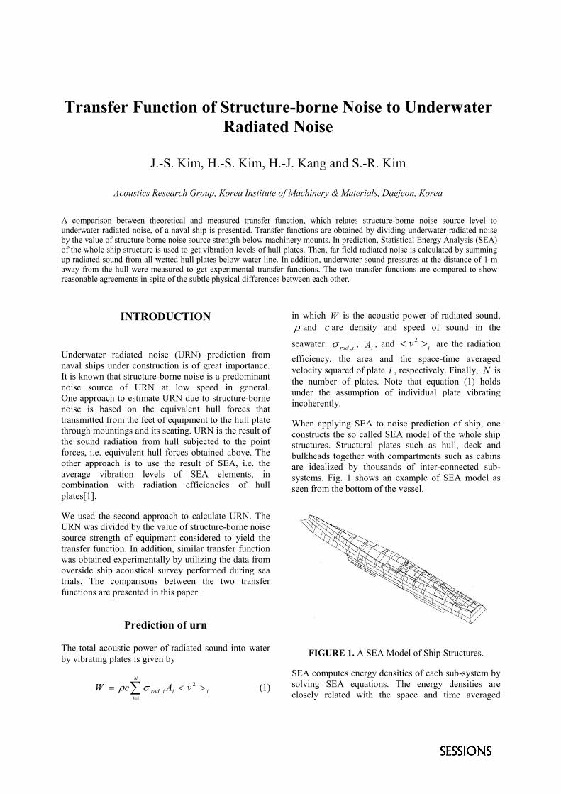
Transfer Function of Structure-borne Noise to UnderwaterRadiated Noise

J.-S. Kim, H.-S. Kim, H.-J. Kang and S.-R. Kim

Acoustics Research Group, Korea Institute of Machinery & Materials, Daejeon, Korea

A comparison between theoretical and measured transfer function, which relates structure-borne noise source level tounderwater radiated noise, of a naval ship is presented. Transfer functions are obtained by dividing underwater radiated noiseby the value of structure borne noise source strength below machinery mounts. In prediction, Statistical Energy Analysis (SEA)of the whole ship structure is used to get vibration levels of hull plates. Then, far field radiated noise is calculated by summingup radiated sound from all wetted hull plates below water line. In addition, underwater sound pressures at the distance of 1 maway from the hull were measured to get experimental transfer functions. The two transfer functions are compared to showreasonable agreements in spite of the subtle physical differences between each other.

INTRODUCTION

Underwater radiated noise (URN) prediction fromnaval ships under construction is of great importance.It is known that structure-borne noise is a predominantnoise source of URN at low speed in general.One approach to estimate URN due to structure-bornenoise is based on the equivalent hull forces thattransmitted from the feet of equipment to the hull platethrough mountings and its seating. URN is the result ofthe sound radiation from hull subjected to the pointforces, i.e. equivalent hull forces obtained above. Theother approach is to use the result of SEA, i.e. theaverage vibration levels of SEA elements, incombination with radiation efficiencies of hullplates[1].

We used the second approach to calculate URN. TheURN was divided by the value of structure-borne noisesource strength of equipment considered to yield thetransfer function. In addition, similar transfer functionwas obtained experimentally by utilizing the data fromoverside ship acoustical survey performed during seatrials. The comparisons between the two transferfunctions are presented in this paper.

Prediction of urn

The total acoustic power of radiated sound into waterby vibrating plates is given by

in which W is the acoustic power of radiated sound,� and c are density and speed of sound in the

seawater. irad ,� , iA , and iv ��2 are the radiation

efficiency, the area and the space-time averagedvelocity squared of plate i , respectively. Finally, N isthe number of plates. Note that equation (1) holdsunder the assumption of individual plate vibratingincoherently.

When applying SEA to noise prediction of ship, oneconstructs the so called SEA model of the whole shipstructures. Structural plates such as hull, deck andbulkheads together with compartments such as cabinsare idealized by thousands of inter-connected sub-systems. Fig. 1 shows an example of SEA model asseen from the bottom of the vessel.

FIGURE 1. A SEA Model of Ship Structures.

SEA computes energy densities of each sub-system bysolving SEA equations. The energy densities areclosely related with the space and time averaged

)1(2

1, i

N

iiirad vAcW ��� �

�

��

velocity squared, appeared in (1), for plate members.Therefore, we can use the SEA solutions directly toobtain the acoustic power radiated into the water fromthe wetted hull surface by using (1). As for radiationefficiencies of plates in contact with water like ship’shull, one can use the formula suggested by Uchida etal. [2].

Once the acoustic power is obtained, the far fieldpressure is given as follow under the assumption ofspherical spreading from point source.

)2(/2 22 cprW ���

After some calculations, the radiated pressure at 1 mapart from the source is given as

)3(54log10 ���� fLL wp

where, pL is the URN level (dB ref 1 �Pa, 1 m, 1 Hz),

wL is the acoustic power level (dB ref 10-12 W),and f� is the bandwidth.

Structure-borne noise transfer function

We defined the structure-borne noise transfer functionas

)4(ap LLTF ��

in which TF is the transfer function of structure-bornenoise, pL is the URN as described in (3), and aL isthe 1/3 octave band acceleration level (dB ref 10-5

m/sec2) at the position below the equipment mount.

During overside acoustic surveys, a hydrophone wasplaced 1 m apart from the hull to measure theunderwater sound pressure induced by the operation ofindividual equipment. At the same time, accelerationsbelow the equipment mount were also recorded.

We calculated the experimental transfer functionsusing these two measurement results, and comparedwith those of theoretical values in Fig. 2 and 3 for adiesel generator and a pump, respectively.

Concluding remarks

It is an interesting fact that the two transfer functionscompare reasonably well in spite of the differences in

FIGURE 2. Transfer Function : Diesel Generator.

FIGURE 3. Transfer Function : F.O.T. Pump.

exact definitions, i.e. prediction for far field andmeasurement done near hull plates. This phenomenon,although not conclusive, could be utilized whenanalyzing noise transmission path of machinery withrelatively small source levels or refining URNprediction method in an effective way.

ACKNOWLEDGMENTS

This work was partially supported by a grant from theCritical Technology project of the Ministry of Scienceand Technology, Korea.

REFERENCES

1. Hyun-Sil Kim, Jae-Seung Kim, Hyun-Ju Kang and SangRyul Kim, An application of SEA to ship noiseprediction, NOVEM International Conference, LyonCongress Center, 31 Aug. – 2 Sep., 2000.

2. S. Uchida, Y. Yamanaka, K. Ikeuchi, K. Hattori and K.Nakamachi, Prediction of underwater noise radiatedfrom ship’s hull, Bulletine of the Society of NavalArchitectures of Japan, No. 686, 36-45, (1986).

Flow Noise and Functional Models ofWall-Turbulent-Pressure

E. B. Kudasheva, L. R. Yablonikb

aSpace Research Institute of Russian Academy of Sciences, 117997 Moscow, Russiab I.I.Polzunov Scientific and Development Association on Research and Design of Power Equipment (NPO

CKTI)., S.-Petersburg, Russia

Two models of spatial characteristic functional of near-wall-turbulent pressure fluctuations are suggested and analyzed in view todevelop the method of experimental investigation of characteristic functional of near-wall turbulent pressure field. They are aGaussian model for jet flow and a Poissonian model for turbulent boundary layer. The functional approach permits to reduceexperimental investigation of turbulent pressure field characteristic functional to measuring a limited number of parameters anddependencies typical of the studied turbulent flow- against type.

EXPERIMENTAL METHOD OFCHARACTERISTICAL FUNCTIONAL

From Haddle and Skudrzyk paper[1] the response of aflush-mounted transducer to the pressure field in aturbulent boundary layer is known as the flow noise.Themost comprehensive are continual statistical models ofspatial structure of wall-pressure-fluctuations р(x)described by characteristic functional Φ[υ(x)] =<exp{i∫υ(x))p(x)dx}> and representing full statisticaldescription of a random pressure fluctuation field p(x,t).The present work analyses forms of analyticrepresentation of characteristic functional of turbulentpressure fluctuations. The functional approach developedby the authors of the present work [2] makes it possibleto obtain an exhaustive description of random field p(x)based on experimental investigation of characteristicfunctional of wall-turbulent pressure field. Estimatedexperimentally, characteristic functional Φ[υ (x)] isdefined on a set of functional arguments υ = λ K(x),where λ is the sensitivity of a transducer, K (x) is itspulse characteristics. Because of the sensor averagingeffects the characteristic function of the transducer signalφs(λ) = <exp (iλs)>gives the characteristic functional:

φs (λ) = <exp {i ∫ λ K (x) p (x) dx}> = Φ[λK(x)]. (1)

For probes with rather small reception surfaces so thatpulse characteristics is reduced to delta-function λ K (x)� λ γ0 δ (x – x0), the characteristic functional is : φs (λ) ≈<exp {i λ γ0 p(x0)}> = φp (λ γ0) (2)

corresponding to single-point probability distribution ofpressure. In the case the receiver is an array of n pointprobes with sensitivity λ, pulse characteristics :

λ K (x) � ∑ λ i γ0 δ (x – x i) ≡ ∑ γ i δ (x – x i) , (3)

and the characteristics functional is transformed into acharacteristics function of n-dimensional distribution ofprobability:

φs (λ 1 ….. λ n ) = φ x1 ... x n (γ1..… γn) (4)

THE CHOICE OF FUNCTIONALMODELS OF TURBULENT PRESSURE

Turbulent flows different in statistical nature of turbulentfluctuations generation are described by differentfunctional models. In the case of a jet flow when pressurefluctuations are caused by external turbulence and thedistance between the sources and the point ofobservation is not too small, the well-known integraldescription of pressure fluctuations allows to representnear-wall fluctuations as a sum of great number ofstatistically independent components related to differentzones of the turbulent flow. Random values of the kind,as a rule, have asymptotically normal distribution thatimplies a model of a Gaussian field whose characteristicfunctional has the form

ΦG [υ (x)] = exp {-½ ∫∫ υ(x1)υ(x2)R (x1, x2)dx, dx2} (5)

Here R(x1, x2)is the correlation function R=<p(x1)p(x2)>.The characteristic function of the signal of transucer:

φ sG = ΦG [� K(x)] = exp [- λ2 / 2 ∫ � (�) R (�) d� ] , (6)

� (�) = ∫ K(x) K(x+�)dx is the impact function of thereceiver. The wave form of the characteristic function isφsG = exp [- λ2/2∫S(k)E(k)dk] , (7)where S(k) = ∫�(�)exp(-ik�)d� is the wave characteristic

of the receiver, E(k) is the frequency-wave spectrum ofthe turbulent pressure fluctuations.

Another functional model can be suggested for pressurenearfield in the turbulent boundary layer. In contrast tojet flows, near-wall pressure fluctuations in turbulentboundary layer is essentially determined by spontaneoussplashes accompanied by surges of the liquid from thewall towards external area of the flow. Assumingstatistical independence of the splashes and their uniformprobability distribution over the surface, one can roughlydescribe the turbulent pressure fluctuations using thePoissonian statistics :

ΦP [υ (x)] = exp {�∫[χ(∫g(x-y)υ(x)dx)–1]}. (8)

Here � is mean number of splashes for the unity of area,χ(µ) is the characteristic function of the probabilitydistribution of pressure fluctuations P in the kernel of asplash, g (r) is impact function of the splash (g (0) = 1)defining spatial correlation links:

R (r) = � <Ρ2> ∫ g ( ρ) g (ρ + r) dρ . (9)

The signal characteristic function of homogeneousreceiver of the area of S0 (in this case, at the apertureK(x) = K0 = const) in a Poissonian field is presented as

φsP(�) = exp {�∫ [χ (λ K0 ∫S0 g (x – y) dx) –1] dy}. (10)

For small S0, when receiver can be considered point-shaped, we get from the above expression

φsP1(�) = exp {�∫ [ χ (λ γ0 g ( ρ) ) –1] dρ }. (11)

If in homogeneous field, the area of the receiver surfaceS0 dramatically exceeds the area σ0 = ∫ g(ρ)dρ of theimpact zone of the spontaneous splash, then, in line with(10),

φsP(�)� exp {� S0 [ χ (λ γ0 σ0 / S0) –1] }. (12)

Since <Ρ>=0, it follows that for large area of the receiversurface S0/σ0 >>1 and the corresponding distributionapproaches Gaussian distribution :

φsP2(�) = exp [-½ λ2 γ02 <P2> νσ2

0 /S0 ] . (13)

CONCLUDING MODEL

One can assume that the variety of stochastic regimes ofwall-turbulent pressure fields, including those inboundary layer with turbulence at its external limit takeninto account, may be represented by a superposition of

functional models studied in the work, or theirmodifications. In the case Gaussian and Poissoniancomponents can be considered statistically independent,the structure of characteristic functional Φ [υ (x)] isobviously, within the given reasoning, a product ofexpressions (5,8):

Φ [υ (x)] = exp{-½ ∫∫ υ (x1) υ (x2) RG (x1, x2) dx, dx2}*

exp {�P ∫ [χP ( ∫ gP(x-y) υ (x) dx) –1] }. (14)

It has been show that the suggested functional approachpermits to reduce the task of experimental investigationof the characteristic functional to measuring a limited setof parameters typical of a given type of turbulent flows.They are correlation function of turbulent pressurefluctuations RG(x1,x2) for Gaussian field and thedependencies �P, χ(µ); gP(ρ) for Poissonian component ofturbulent pressure field.

REFERENCES

1.Haddle G.P. and Skudrzyk E.J.,J. Acoust.Soc.Amer., 46, 130-157(1969).

2. Kudashev E.B. and Yablonik L.R., Phys. Acoustics, 45, 467-471(1999).

The Measurement of Fluctuations of the SignalPropagation Time over Long Acoustic Paths

A.Stromkova, I.Didenkulova, Ya.Karlikb, A.Kazarovaa, L.Lyubavina,E.Pelinovskya

aInstitute of Applied Physics, Nizhny Novgorod, RussiabMorphispribor, St. Petersburg, Russia

Acoustic waves can propagate in the ocean over basin scales and therefore can serve as a unique tool for diagnostics ofocean processes including internal waves, tsunami etc. The present paper describes results of the experiment on long-range sound propagation at the 4800 km acoustic path Hawaii-Kamchatka. Pseudo-random signals (M-sequence) at thecarrier frequency of 75 Hz were radiated by a source deployed near Hawaii. The signal frequency band was 37.5 Hz,which allows one to measure travel time with accuracy of about 30 ms. In our measurement the phase-differencealgorithm was used. The accuracy of travel time measurement with this method was significantly improved. It wasobserved that tides produce strong oscillations of travel time The results of experiments were found to be in good agreewith theoretical calculations based on the ТХРО5 model for tides.

1. INTRODUCTION

Acoustic waves can propagate in the ocean overbasin scales and therefore can serve as a unique toolfor diagnostics of ocean processes: tides, eddies,currents, tsunami, internal waves, etc [1]. The mainphysical reason of the influence of ocean processes atacoustic signal is water motion, which results in thechange of the acoustic signal travel time. Therefore,the measurement of acoustic travel time changes andtheir identification are the main problems. Acoustics iswidely used for ocean study. It is evident that for highspatial-time and frequency resolution high frequencyacoustic waves would be used. But sound attenuationrapidly increases with frequency that makesimpossible the use of high-frequency sound (aboveseveral hundred Hz) for monitoring over distances ofabout several tens km. Only very low frequency sound(below 100 Hz) can propagate over basin scales.Traditional way to measure the travel time variations isbased on the use of the phase method and harmonicacoustic signals. The phase is related with the traveltime through the sound velocity and the propagationpath. However, sound propagates in the ocean bymany paths – rays, which produce many acousticarrivals at the receiver. Such arrivals usually overlapeach other and therefore can not be separated.Consequently, the acoustic phase can give onlyinformation on ray-averaged fluctuations for traveltime. Relatively recently more complex signal beganto use in the ocean acoustics – so called M-sequence.The M-sequence signal being long in time has wide

spectrum, and can be compressed in time by the use ofcorrelation technique. The M-sequence signal allowsone to measure travel time variations for differentpaths or path-groups separately. In the present paperwe describe results of experimental study of soundpropagation over 4800 km. For detection of travel-timevariation the novel approach is used based ofdifference phase method applied to the M-sequencesignals.

2. METHOD OF ACOUSTIC TRAVELTIME MEASUREMENT

Let a signal, which is the harmonic carrier modulatedin phase with the M-sequence is emitted by the soundsource. The receiving acoustic signal is the sum ofsignals arrived by different paths. To analyse thereceived signal one need to divide the signal by partsof duration equalled to the M-sequence duration T. Foreach of these parts defined as the k-th part of thereceived signal the cross-correlation function with thereplica of the radiated signal is

( ) ( ) ( )k

k

t T

k kt

b y t M t dtτ τ+

= −∫ , (1)

where yk(t) is the k-th part of the received signal, M(t)is the replica of the emitted signal, and T is the M-sequence duration.

One can introduce the function ρk (m) as follows

0 ( )

( ) ( ) ( )

( ) ( )k k m

k k k mT

ik k m

T

m b b d

e h h dω τ τ

ρ τ τ τ

τ τ τ+ ∗

∗+

−+

= =

=

∫

∫, (2)

where τk is the travel time, hk (τ) – the pulse responseof the acoustic channel during k-sequence. The phaseof the function ρk (m) is ϕk(m)=ω(τ k-τk+m). For correctmeasurements of the travel time it is necessary that thephase ϕk (m) for the time interval mT does not exceedπ. If θ is the travel time, an approximate expression forthe derivation of the travel time is

0

( ) ( , )2

d k n kdt f nT

θ ϕπ

≈ . (3)

Thus, the phase difference method is based onmeasurements of the phase ϕk(m) that is the phasevariations between acoustic transmissions. The traveltime variations are directly related to the phasevariations.

3. EXPERIMENT AND RESULTS

The experiment on long-range sound propagationwas conducted at the 4800 km Hawaii-Kamchatkaacoustic path. Pseudo-random signals (M-sequence) atthe carrier frequency of 75 Hz were radiated by asource deployed near Hawaii. The signal frequencyband was 37.5 Hz, which allows one to measure traveltime with accuracy of about 30 ms. The sound receiverwas installed near Kamchatka. Travel time fluctuationswere studied for the time period of about one year. It isworthy to note that the signal to noise ratio at thehydrophones in the experiment was below -10 dBmeasured in the signal frequency band. Measured fluctuations of the travel time werecompared to calculated fluctuations. The calculationwas made with the use of the global inverse tidalmodel TXPO5.1 [2]. The acoustic path was dividedinto 10 segment of about 500 km length. For eachsegment tidal current was supposed to be constant,which was calculated with the PXPO5.1 model formiddle point of the segment. We neglected multipathacoustic propagation in calculations. The travel timederivative was estimated by calculation of the traveltime in 6 minute interval. The experimental andcalculated data are shown in Figure 1. As it is seen from Figure 1, even such a simplemodel for acoustic travel time fluctuations due to tidalcurrents demonstrates good correlation with the

experimental data. The coefficient of correlationbetween them achieves 0.6-0.7.

0 5 10 15 20 25 30 35-1

-0.8

-0.6

-0.4

-0.2

0

0.2

0.4

0.6

0.8

1x 10-5

Der

ivatio

n of

trav

el ti

me

(s p

er s

)

Experiment number

ExperimentCalculation

FIGURE 1. The derivative of the travel time overacoustic path. Experiment and calculation based on thetide model.

4. CONCLUSION

In this paper the phase-difference algorithm based onthe use of M-sequence signal for detection of smallfluctuations of the acoustic travel time was described.The accuracy of travel time measurement with thismethod was significantly improved. Experiment onlong range sound propagation from Hawaii toKamchatka revealed that tides produce travel timeoscillations having amplitude of up to 0.2 s. The mainphysical mechanism of influence of tides on traveltime is tidal currents. The proposed method can beused for detection of water motion due to tsunami.

ACKNOWLEDGMENTS

This work was supported by RFBR (01-05-64426,01-05-64162, 00-15-96741).

REFERENCES

1. Munk W. and Wunsch C., Deep Sea Research, 26A, 123-161 (1979).

2. Egbert G. and Erofeeva S., “Efficient inverse modelling ofbarotropic ocean tides. Global Inverse Solution TPXO.5.1.”in http://www.oce.orst.edu/po/research/tide

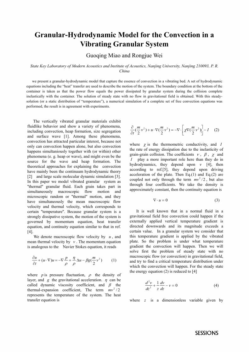
Granular-Hydrodynamic Model for the Convection in aVibrating Granular System

Guoqing Miao and Rongjue Wei

State Key Laboratory of Modern Acoustics and Institute of Acoustics, Nanjing University, Nanjing 210093, P. R.China

we present a granular-hydrodynamic model that capture the essence of convection in a vibrating bed. A set of hydrodynamicequations including the “heat” transfer are used to describe the motion of the system. The boundary condition at the bottom of thecontainer is taken as that the power flow equals the power dissipated by granular system during the collision completeinelastically with the container. The solution of steady state with no flow in gravitational field is obtained. With this steady-solution (or a static distribution of “temperature”), a numerical simulation of a complete set of free convection equations wasperformed, the result is in agreement with experiments.

The vertically vibrated granular materials exhibitfluidlike behavior and show a variety of phenomena,including convection, heap formation, size segregationand surface wave [1]. Among these phenomena,convection has attracted particular interest, because notonly can convection happen alone, but also convectionhappens simultaniously together with (or within) otherphenomena (e. g. heap or wave), and might even be thesource for the wave and heap formation. Thetheoretical approaches for explaining the convectionhave mainly been the continuum hydrodynamic theory[2] and large scale molecular dynamic simulation [3].In this paper we model vibrated granular system as''thermal'' granular fluid. Each grain takes part insimultaneously macroscopic flow motion andmicroscopic random or ''thermal'' motion, and theyhave simultaneously the mean macroscopic flowvelocity and thermal velocity, which corresponds tocertain ''temperature''. Because granular system is astrongly dissipative system, the motion of the system isgoverned by momentum equation, heat transferequation, and continuity equation similar to that in ref.[4]. We denote macroscopic flow velocity by u , andmean thermal velocity by v . The momentum equationis analogous to the Navier Stokes equation, it reads

)2

()( 2vmgupuutu β

ρη

ρ−∆+−∇=∇⋅+

∂∂ (1)

where p is pressure fluctuation, ρ the density oflayer, and g the gravitational acceleration. η can becalled dynamic viscosity coefficient, and β thethermal-expansion coefficient, The term 2/2mvrepresents the temperature of the system. The heattransfer equation is

Ivmvmuvmt

−

∇⋅−∇=∇⋅+

∂∂ )

2()

2()

2( 222 χ (2)

where χ is the thermometric conductivity, and Ithe rate of energy dissipation due to the inelasticity ofgrain-grain collision. The coefficients ν , β , χ andI play a more important role here than they do inhydrodynamics, they depend upon v [4], thenaccording to ref.[5], they depend upon drivingacceleration of the plate. Then Eq.(1) and Eq.(2) arecoupled not only through the term 2/2mv , but alsothrough four coefficients. We take the density isapproximately constant, then the continuity equation is 0=⋅∇ u (3)

It is well known that in a normal fluid in agravitational field free convection could happen if theexternally applied vertical temperature gradient isdirected downwards and its magnitude exceeds acertain value. In a granular system we consider thatthis temperature gradient is applied by the vibratedplate. So the problem is under what temperaturegradient the convection will happen. Then we willsolve first the problem of steady state with nomacroscopic flow (or convection) in gravitational field,and try to find a critical temperature distribution underwhich the convection will happen. For the steady statethe energy equation (2) is reduced to [4]

012

2

=−+ vdzdv

zdzvd (4)

where z is a dimensionless variable given by

λ/)( ' xhz −= as in ref.[4]. The boundary condition atfree surface ( hz = ) is taken as

02 ==hx

vdxdK (5)

this means that the energy flux vanish at free surface.As to the boundary condition at bottom of the container( 0=x ), we consider as follows. In ref.[5] we use amodel of a single sphere colliding completely inelasticwith a massive sinusoidally oscillating plate to describethe motion of a layer of vibrated granular material, andobtained the power input P by the plate for each grainas a function of acceleration of the plate (showngraphically in figure 1). So here we use

FIGURE.1: (a) The mean power input, P , for each grain,as a function of dimensionless acceleration of the plate.

this P as power input for each grain from theboundary 0=x , and obtain the boundary condition

PmvdxdK

x

==0

2 )21( (6)

The solution to (4) are the modified Bessel function ofzero order, )(0 zI and )(0 zK .

)()( 00 zBKzAIv += (7)

Here hx → corresponding to 0→z . As the function)(0 zK is singular here, )(zv must be given by )(0 zI

alone, i. e.

)(0 zAIv = . (8)

Insert this into the equation (6), we have

2/1

00 )/(

=dxdImKIpA (9)

Principle, we could use the general theory for freeconvection with the temperature distribution (8) toobtain the condition under which the convection couldhappen. But in fact it can hardly be done so. We canonly use numerical method to calculate it. The resultsare shown that nothing happens for 1<Γ . For 1>Γand reaches some critical value the convection doeshappen. Figure 2 shows a convection pattern of twodimensional system, which are in quality agreementwith experiment.

FIGURE.2: A convection pattern of two dimensionalsystem.

This work is supported by the Special Funds forMajor State Basic Research Projects and NationalNatural Science Foundation of China through GrantsNo. 10074032, 19834040 and 19874029.

REFERENCES

1. H. M. Jaeger, S. R. Nagel and R. P. Behringer, Phys. Today,49(4), 32-38 (1996).

2. Marc BourZutschky and Jonathan miller, Phys. Rev. Lett.74, 2216-2219 (1995); Hisao Hayakawa, Su Yue, andDaniel C. Hong, ibid 75, 2328-2331 (1995).

3. Rosa Ramirez, Dino Risso, and Patricio Cordero, Phys.Rev. Lett. 85, 1230-1233 (2000).

4. P. K. Haff, J. Fluid Mech. 134, 401-430 (1983).5. Guoqing Miao, Lei Sui, and Rongjue Wei, Phys. Rev. E 63,

031304 (2001).

2 4 6 80

2

4

6

8

10

Γ

P (1

0-7J/

s)

0 5 10 15 200

2

4

6

88

10

12

X

Y

The Use of an Equivalent Medium for a Coupled Inversionin Underwater Acoustics

J.C.Le Gaca, M.Aschb

a Centre Militaire d’Océanographie, EPSHOM, B.P.30316, 29603 Brest Cedex, Franceb Laboratoire ANAM/MNC, Institut des Sciences de l’Ingénieur de Toulon et du Var, B.P.56, 83162 La Valette du

Var Cedex, France

Abstract : The paper describes a shallow water geoacoustic inversion scheme based on a model based matched impulse response.The concept is derived from a previous paper [2] which presents an equivalent medium approach. The technique exploits the moststable part of the impulse response of the acoustic channel, giving robust estimates of geometrical and geoacoustic parameters.

INTRODUCTION Bottom properties are essential in the frame ofshallow water acoustics, especially for very lowfrequencies. Several approaches have been developedin the last few years leading to good estimates ofgeoacoustics properties. A new trend lies in the use ofbroadband signals received on sparse arrays, possiblyreduced to a single hydrophone[1]. Bottom propertieshave shown to be robustly and efficiently retrievedfrom measured impulse responses. This paper presents an approach following previouswork explained in [2]. The aim of this previous workwas to determine an equivalent medium and it wasapplied to the INTIMATE96 sea cruise data set [3].The idea of “equivalent medium” means that thebottom thus determined behaves as the true medium inthe limit of an acoustical application (a kind of“through the sensor” approach). The equivalentmedium concept consists in assessing the mainparameters when using a sonar system rather thanfinding relevant physical parameters. The frame of thisgeoacoustic inversion method, mainly based on ananalytical development of the reflection coefficient,was limited to simple equivalent media (semi infinitefluid half spaces) and questionable in the case of highfrequency dispersive true media. We propose in thisarticle a generalization of this previous approach.

GEOACOUSTIC INVERSION SCHEME The INTIMATE96 data set consists of broadbandsignals (300 to 800 Hz chirps, 2s duration, repeatedevery 8s) received on a 4-hydrophone vertical array.We exploit a range-independent phase shown on Figure1. Matched filtering (cross correlation of the receivedand the emitted signals) was applied. The envelopes ofthe estimated impulse response thus obtained were thenextracted (Figure2). The received sequences weredivided into two parts. The first spikes are direct pathsrefracted in the thermocline with a small number ofbottom reflections. They were highly sensitive to the

sound speed profile. The second part, quite stable,exhibited a multipath structure of bottom-surfacereflected rays supposed to carry most of theinformation on the bottom properties.

Inversion of Geometrical ParametersThe exact geometry of an experiment (distancesource/receivers [D], source [Zs] and receiver [Zr]depths, water column depth [H]) is often unknownprecisely due to operating modes and the lack of directmeasurements of these parameters. For example, thelocalization of the source is quite difficult when it istowed by a boat. Geometrical parameters must be wellknown in order to perform a reliable geoacousticinversion. Thus, we applied a generalization of alinearized inversion scheme presented in [4] in order torefine the a priori knowledge of the geometricalparameters. This scheme, not explained in detail in ourpaper, exploits the travel times of 12 identified bottom-surface reflected rays from the 115m depthhydrophone. It takes advantage of the fact that theserays are slightly deviated by the sound speed profile.

ResusummeaThey

csurf=1520 m/s

mm

h1 = 2msilty sand

m

zr3~115 mD~5.5 km

cp = 1650m/s ρ = 1.8 kg/dm3

αp = 0.36 dB/m/kHz

bot

shell,gravel and sand

cp = 1750m/s ρ = 2. kg/dm3

αp = 0.28 dB/m/kHz

F

ltmn

limestone

cp = 3000m/s cs = 1600 m/s ρ = 2.4 kg/dm3

αp = 0.07 αs = 0.25 dB/m/kHz

c =1508 m/s

IGU

s oarizparmat

zs~93

RE 1. Experimentaparameters for the r

f the inversion fred in Table 1. Tameters are plottech the measured tr

H~135

l set up and enviroange independent

om 20 starting ravel times obd on Figure 2 (avel times very

h2 = 0.5m

zr1~35

zr2~105 m

nmentalleg

models aretained withblack bars).well.

Table 1. Inversion of geometrical parametersParameter Mean (m) Standard Deviation (m)

D 5629.5 0.4H 134.82 0.13Zs 90.95 0.14Zr 115.91 0.20

Geoacoustic Inversion Once geometrical parameters have been preciselydetermined, the geoacoustic inversion can beperformed. The geoacoustic model we looked for wasa simple fluid half-space in order to compare it to theresults given in [2].

3.75 3.8 3.85 3.9 3.95 4 4.05 4.1 4.15

0

0.1

0.2

0.3

0.4

0.5

0.6

0.7

Time (s)

Impu

lse re

spon

se en

velop

e

FIGURE 2. Typical INTIMATE96 envelope of the impulseresponse on the 115 m depth hydrophone

The algorithm is based on the comparison of the peaklevels of each bottom-surface reflected path betweenthe measured impulse response and a simulatedimpulse response. The stable part of the impulseresponse envelopes (after 3.75 s) is normalized to unitenergy, giving the following objective function to beminimized :

niipipcfi

sl

mlp �� =−= 1,)()(),,( ρα

where plm is the level of a measured peak, pl

s is thelevel of the corresponding simulated peak, n is thenumber of paths taken into account (for t>3.75s). The simulated impulse responses were computedwith the GAMARAY ray model [5] which providesgood estimates of the impulse response in comparisonwith normal mode models, even near the critical angle(which is essential for our inversion scheme), for thiskind of environment. A parametric study showed thatthe objective function had only a single globalminimum, which allowed us to use the Nelder andMead simplex optimization algorithm in order to findcp and α [6].The mean estimates of the most sensitive geoacousticparameters were : 1678.8m/s for cp, 0.35 dB/m/kHz forα , and 1.86 kg/dm3 for ρ. The density was deducedfrom cp. Twenty starting values were chosenstochastically within the following bounds {[1550 ;1850]m/s and [0.3 ;0.7]dB/m/kHz} (Figure 3).These mean estimates were in good accordance with aweighted sum of the superficial layers parameters of

the true medium. Furthermore, the inversion was quitestable in comparison to the one performed in [2] (forα). Except for very few localized frequencies, thecomparison of simulated coherent losses at 5.63 kmwith the true medium and the equivalent one proved tobe in very good accordance between 200 and 800 Hz(not shown in this paper). Between 50 and 200 Hz, thesame comparison showed greater differences due to theinteraction of the basement (Figure 4). The accordancefor the phase was not as good which is not surprising:the half space fluid medium is unable to render thesame complexity of phase shift as the true medium atbottom reflections.

0 20 40 60 80 1001550

1600

1650

1700

1750

1800

1850

Cp (m/

s)

Number of function evaluation0 20 40 60 80 100

0.2

0.3

0.4

0.5

0.6

0.7

0.8

0.9

Number of function evaluation

Alpha (

dB/m/k

Hz)

FIGURE 3. Geoacoustic inversion from 20 starting models

Loss

es (d

B)

−70

−65

−60

−55

Depth (m)

True medium

20 40 60 80 100 120

50

100

150

200

250

300

Depth (m)

Freq

uenc

y (H

z)

Equivalent medium

20 40 60 80 100 120

50

100

150

200

250

300

FIGURE 4. Coherent losses for true and equivalent media

CONCLUSIONA simple and robust approach for geoacoustic inversionhas been presented in this paper. It is shown to be morestable than previous work in [2]. It shows that theequivalent medium is relevant in the case ofINTIMATE96 context for coherent losses between 200and 800 Hz.

REFERENCES1. Hermand, J.P., IEEE J.Oceanic Eng. 24,41-66 (1999)2. Demoulin, X., et al., Estimating equivalent bottom

geoacoustical parameters from broadband inversion in Proc.ECUA2000, M.E.Zakharia et al. eds. ,Lyon,France,2000,pp.191-196

3. Stephan, Y., et al., Acoustical effects of internal tides onshallow water propagation : an overview of the INTIMATE96experiment, in Exp. Ac. Inv. Methods for Exploration of theShallow Water Environment, Caiti et al. eds, KluwerAcademics Publishers (2000), pp.19-38

4. Dosso, S., et al, J.Acoust.Soc.Am. 104,846-859 (1998)5. Westwood, E.K., et al., J.Acoust.Soc.Am. 81,1752-1761 (1987)6. Press,W.H., et al., Numerical Recipes in C, Cambridge

University Press (1992)

1. Introduction Parabolic Equation Methods (called Beam PropagationMethod in branches of optics), in which an acoustic fieldsolution can be determined by solving the one-way op-erator equation for the forward-propagating field, are pow-erful design tools for underwater wave propagation prob-lems. A great number of PEM’s have been proposed bypioneers since its inception [1,4,5]. The advantage of theFD-PEM is its simple numerical implementation and canbe simulated within a reasonable cpu-time and memory.On the other hand, the method has several drawbacks be-cause it is approximation to the Helmholtz’s wave equa-tion neglected backward-wave. In order to overcomeabove drawbacks, a new approach for developing the PEmethod in time-domain is to use the wave equation basedon slow-varying envelope approximation and is calledthe TD-Beam Propagation Method in optics field [2,3].Based on this SVEA, an acoustic short pulse propaga-tion has been applied to the wave equation simultaneouslyleading to an algorithm suitable for studying forward wavepropagation, wide angle of diffraction and reflection. Inthis paper, we propose a very efficient time-domain para-bolic equation method (TD-PEM). The aim of this paperare: (1) to derive a new formalism for the pulse propaga-tion in time domain; and (2) to demonstrate its possibil-ity to treat underwater acoustic pulse propagations.

2. Basic formalism For the sake of simplicity of formulation of TD-PEMbased on SVEA , we restrict ourselves to the two dimen-sional problem and the wave equation in Cartesian coor-dinates. For underwater acoustic wave propagation prob-lems, the wave equation is given by

∇×∇× + =ψ∂ ψ

∂

n

c t

2

2

2

20 (1)

Proposal of FDTD-PE Method with Slow Varying EnvelopeApproximation for Underwater Acoustic Pulse Propagation

Tetsuo Anada, Takenobu Tsuchiya, Nobuyuki. Endoh (Kanagawa University)Toshio Tsuchiya and Toshiaki Nakamura (JAMSTEC)

3-27 Rokkakubashi Yokohama, 221-8686 JAPAN E-mail: anada@cc.kanagawa-u.ac.jp

In this paper, a new finite-difference time-domain PE method based on the slow-varying envelope approximation isproposed for the analysis of forward wave propagation, diffraction and reflection and given for short pulse propaga-tion problems in underwater acoustics. The advantage of the FDTD-PEM proposed here is its simple numericalimplementation and can be analyzed within a reasonable cpu-time and memory. In order to improve the accuracy andefficiency of the method, the computational spatial discretization of second-order differential is replaced by theDouglas operator scheme, which the truncation error of O(∆x)4 is ensured in the depth direction.

where t is time, n(r,t)=c0/c(r,t) is the refractive index, c0

and c is the reference sound speed, the sound speed inunderwater acoustics. In comparison with a carrier fre-quency, the signal frequency will be regarded as a slowwave propagation. By applying SVEA to the time termof the wave equation and substituting a solution of theform ψ ϕ ω( , ) ( , )r t r t e j t= ⋅ − into Eq.(1), the following time-domain wave equation is obtained:

− − =−∇×∇× +n

c tj

n

c t

n

c

2

2

2

2

2

2

2 2

22

∂ ϕ

∂

ω ∂ϕ

∂ϕ

ωϕ (2)

where ω is the angular frequency (carrier frequency) .The first term on the time is much smaller than the sec-ond term. With above first-order approximation, the re-duced wave equation may be written as:

− = + +22

2

2

2

2

2

2 2

2j

n

c t x z

n

c

ω ∂ϕ

∂

∂ ϕ

∂

∂ ϕ

∂

ωϕ (3)

While, for acoustic wave propagation confined in thex-z plane with z-propagating beam, the paraxial waveequation is rewritten as follows:

− = + + −( )20

2

2

2

2 0

2 2 2jk nz x y

k n nb b

∂ϕ

∂

∂ ϕ

∂

∂ ϕ

∂ϕ (4)

where nb is the reference index, k0 is the wave number. Comparing with Eq.(3) and (4) , Eq.(3) and Eq.(4)have the same form. It is quite obvious that PE codescan be extended to solve the time-domain PE equationin the slow-wave approximation. Therefore, we can besolved by using Alternating Directing Implicit Method(so called operator splitting method) for obtaining thesolution of Eq.(3). The ADI method can be applied to lead to a programsuitable for Eq.(3). The principle is to use two differentequations that are used in turn over successive time-stepseach of duration ∆t/2. That is, the first equation is solved

implicitly only in the x-direction and the second only inthe z-direction. In addition, to improve the accuracy ofthe simulation, the Douglas operator scheme firstly usedby Lee, et al is applied. As a result, we can easily obtainthe high accuracy six-point scheme (then, the truncationerror is the fourth-order) and lead to a tridiagonal systemof complex linear equations[6].

ρ∂

∂ ρ

∂

∂

δ

αδ( )

( )x

x x x xx

x

1 1

12

2

2

=+∆

α =1

12(Douglas case) , 0 (Crank - Nicolson)

δ ρ φ ρ φ ρ φx i i i

2

1 0 1= − +− − + + ,

ρρ

ρ ρρ ρ ρ± + −=

+ ±= +

2 ( , )

( , ) ( , ),

x z

x z x x z∆

0

3. Results of simulations In order to demonstrate the validity and usefulness ofSVEA based TD-PEM, we studied the underwater acous-tic pulse propagation in the upsloping seafloor model.The depth of the channel is 100 m and the sound speedand density in the underwater are c=1500 m/s, ρ=1.0 g/cm3, those of sediment layer are 1700 m/s,ρ=1.2 g/cm3 ,the frequency is 500Hz. An acoustic wave packet with adepth profile corresponding to the gaussian beam islaunched at t=0 and z= 50 m. The longitudinal profile ofthe wave pocket along +z propagating direction is alsoGaussian beam with full-width of 10 m. The computa-tional window is 200 m by 1000 m which is discretizedin a 200 by 2000 grid. The time step used is 0.1E-3 [sec].The total duration simulated is 1 [s]. The multimode chan-nel waveguide is supported some guided modes, and isreflected in the boundary of top and upsloping-bottom,and the interference will be occurred. Figure 1 shows thepulse propagation characteristics of the incident-pulsewith Gaussian profile. It is observed that the pulse is con-fined in the underwater column, while the part of the pulsewave is radiated into the upsloping sediment layer. Thevalidity of the present method is confirmed by the coin-cidence with our physical image.

4. Conclusion In this paper a recently developed FDTD-PE methodbased on the SVEA has been given for predicting the pulsepropagations in underewater acoustics. In stead of Crank-Nicolson scheme, the Douglas operator scheme has beenimplemented for the program in order to reduce a trunca-tion error of the finite-difference approximation of the

second order derivative in depth direction. In addition,by combining the higher-order Pade series expansionwith the Douglas operator scheme, it is possible that thepresent method satisfies the accuracy required. In thenear future, the algorithms proposed here will be appliedin practical range dependent 3D problems.

Reference(1)M.A Leontovich and V.A. Fock, Zh. Eksp. Teor. Fiz. 16, pp.557-573, 1946.(2) P.L. Liu, Q.Zhao, and F.S. Choa,”Slow-wave finite-difference beampropagation method”, IEEE Photon., Technol. Lett. vol.7, pp.890-892,1995(3) G.H. Jin, et al, “An improved time-domain beam propagationmethod for integrated optics components,” IEEE Photon. Technol. Lett.vol.9, pp.348-350,1997.(4) M.D.Collins, “A higher-order parabolic equation for wave propa-gation in an ocean overing an elastic bottom”, J.Acoust.Soc.Am.86,pp.1459-1464, Oct.1989.(5) D. Lee, A. D. Pierce, “Parabolic Equation Development in RecentDecade”, J. of Computational Acoustics, Vol.3, No.2, pp.95-173, 1995.(6)J. Yamauchi, et al, “Improved finite-difference beam propagationmethod basd on the generalized Douglas scheme and its application tosemivectoral analysis,”, J. Lightwave Tecnol., no.10, pp.2401-2406,

Oct. 1996.

Fig.1 Pulse propagation in shallow water with upsloping bottom.

0 1000

0

100

200

0

100

200

0

100

200

0

100

200

0 1000

0 1000

0 1000Range[m]

Dep

th[m

]D

epth

[m]

Dep

th[m

]D

epth

[m]

Release boundary conditionat top and bottom.

An Evaluation of Information Transmission UsingUnderwater Auditory Sensitivity in Actual Sea Area

S. Kuwaharaa, K. Oimatsua, K. Kuramotoa, S. Yamaguchib and H. Matsuia

a Japan Coast Guard Academy, Kure-city, 737-8512 Japan b Faculty of Engineering, Yamaguchi University, Ube-city, 755-8611 Japan

Usual divers searching and rescuing in a sunken ship have no communication apparatus because of complexity of the hullconstruction. In such cases, the most simple and effective way for transmitting information is to emit acoustic signals directlyby using an underwater loudspeaker. At this time, it is fundamentally important to research in advance the followingmeasurements: masking of objective signals by ambient noise in the actual sea, evaluating of clearness of voice signal and tonesignal coded by Morse sign. In our research, the above measurements are examined in the actual sea area, using scuba diverswith normal hearing. Measurements of masking effects of auditory ambient noise provide data from which the excitationpattern of the masking stimulus is derived. Evaluations of clearness of voice signal and coded-tone sign are measured bychanging output power levels of the underwater loudspeaker and distances between the loudspeaker and divers.

INTRODUCTION

Many people now enjoy marine sports such as skindiving and scuba diving in sallow water area. Acousticsignals through an underwater loudspeaker can be usedas a simple and effective way of preventing divingaccident. At this time, it is fundamentally importantto research in advance the following measurements:masking of objective signals by ambient noise in theactual sea, evaluating of clearness of voice signal andtone signal coded by Morse sign. In our research, the above measurements areexamined in the actual sea area, using scuba diverswith normal hearing. Measurements of masking effectsof auditory ambient noise provide data from which theexcitation pattern of the masking stimulus is derived.Evaluations of clearness of voice signal and coded-tone sign are measured by five phases of intelligibilityevaluation referring the Radio Regulation (RR) of theInternational Telecommunication Union (ITU).

EXPERIMENT

The research was carried out on actual sea area nearbyJapan Coast Guard Academy, which is usual recreationarea of sea.

Measurement of Minimum Audible Field Underwater

The Minimum Audible Field (MAF) underwater wasdetermined by means of the method of limits.Sinusoidal stimuli at 500, 1000, 2000 and 4000 Hzwere gated ON and OFF with a period of 500 msec.The stimulus-generating equipments and response

units are depicted in Figure 1 consisted on equipmentcommon to audibility threshold experiment. Theresearch was carried out on two subjects who wereexperienced in taking hearing test in air and in water.Each diver was lowered to an ear depth of 2 meters.The divers, wearing open circuit scuba equipment anda wet suit, descended and fixed himself from thetransducer by means of a chest bar and a lead-weightedbelt. Twenty runs were made on each of the twosubjects, and an average of the ascending anddescending runs was made for subjects.

Evaluation of Acoustical Signal

As using voice signals is effective for transmittinginformation to divers, acoustic signals of male andfemale voice sound are emitted directly by using anunderwater loudspeaker. Divers were lowered to an eardepth of 2 meters, and distances between diver’s headand the projector separated were of 20, 50, 100, 160and 200 m. Output levels of the projector wereadjusted adequately by using attenuators

The clearness of voices at each distance wereevaluated by six phases which are referred to thefollowing intelligibility based on RR of ITU: 5excellent, 4 good, 3 fair, 2 poor, 1 bad and 0 no signal.The subjects consisted of two divers who hadexperienced as a radio operator on Japan Coast Guardvessel.

It had been predicted that voice signals were maskedeasily by ambient noise of experimental sea area.Therefore, tone signals coded as ‘QF’ of the Morsesign were adopted because coded tones were notcomparatively masked by noises.

AnalogGate

SignalGenerator

AttenuatorPowerAmp

SoundLevelMeter

DAT

Mic

UnderwaterLoudspeaker

2m

FIGURE 1. Setup for underwater hearing-acuity measurement.

RESULTS

Minimum Audible Field Underwater

In Table 1, some experimental results estimated forminimum audible field (MAF) underwater are reported(dB re 1 �Pa). The MAF levels in quietness measuredby the previous research [1] are expressed in this table.

�As low frequency ambient noises are large (about 95dB/Hz) in the experimental sea area, measured MAFlevels rise compared with quietness levels [2,3]. On theother hand, in high frequency region, MAF levels do notrise very much. Furthermore, it is predicted that MAFlevels increase clearly in high frequency region when adiver was wearing a diving hood [4].

Evaluation of Clearness of Acoustic Signals

In Figure 2 is shown the evaluation of clearness(intelligibility) of the female voice signal and tonesignal varying signal levels at diver’s head pointsreceived. The clearness of voice signal is rapidlydropped with the signal level (slope of dashed line issteep). On the other hand, the clearness of tone signalis slowly dropped (slope is gentle).

In Figure 3, the evaluation of clearness oftone signal varying distances is presented. Data fromfour frequency sequences of increasing distance withfixed source power are shown.

0

1

2

3

4

5

80 100 120 140 160dB

Evaluation of Cle

l=20ml=50ml=100mfitting

(a) Female Voice Signal.

0

1

2

3

4

5

80 100 120 140 160dB

Evaluation of Cle

l=20ml=50ml=100mfitting

(b) Tone SignalFIGURE 2. Evaluation of Clearness (Intelligibility) of(a) Female Voice Signal, and (b) Tone Signal.

0

1

2

3

4

5

10 100 1000Distance (m)

Evaluation of Cle

freq (source power)500Hz (145dB)1 kHz (150dB)2 kHz (150dB)4 kHz (150dB)

FIGURE 3. Clearness of Tone Signal with Fixed SourcePower Levels.

REFERENCES1. K. Oimatsu, K. Kuramoto, S. Kuwahara and

S. Yamaguchi, J. Marine Acoust. Soc. Jpn, 21, 103-109 (1994)(in Japanese).

2. J. E. Hawkins and S. S. Stevens, J. Acoust. Soc. Am., 22, 6-13(1950).

3. S. S. Stevens and H. Davis, “Auditory Masking, Fatigue, andPersistence,” in Hearing, New York, Acoust. Soc. Am., 1938,pp.208-224.

4. S. Kuwahara, K. Oimatsu, K. Kuramoto andS. Yamaguchi, J. Marine Acoust. Soc. Jpn, 25, 86-91 (1998) (inJapanese).

Table 1. Levels of minimum audible field (dB re 1 �Pa).Frequency No Hood With Hood In Quietness

500 Hz 99 dB 100 dB 78 dB1 kHz 100 dB 99 dB 86 dB2 kHz 88 dB 100 dB 89 dB4 kHz 94 dB 119 dB 91 dB

Estimated Model of the Dynamic behaviour of aCavitating Valve

V. VillouvierEDF/DRD/AMV 1 Avenue du Général de Gaulle 92141 Clamart France

The Residual Heat Removal circuit for the French PWR sections comprises two valves which regulate the hot and cold flowrates. These valves operate according to a cavitation system when the circuit is functioning under certain conditions, and theconsiderable excitations which are then created may lead to the cracking of certain small lines located nearby.In order to limit the circuit's vibrations, optimal operating conditions are being sought which would make it possible to reducethe pressure fluctuations at source-level.The valve vibration model which has been developed links the internal acoustic energy to the vibrations measured over the valvebody using local hydraulic variables. Measurements taken on-site in respect of a great many control configurations have made itpossible to readjust the different modelling parameters.Within the context of the RRA circuit, the local valve vibrations are estimated according to the variables governing the globaloperation of the circuit, by using the hydraulics calculation and taking into account the different hydro-acoustic sourcessimultaneously present.

CONTEXTControl description and parameters

Z

YX

12VP

13VP 01DI 26VP

FIGURE 1. Diagram of part of the RRA circuit

The RRA circuit of the French PWR units includestwo hot and cold flow rate control valves. Undercertain operating conditions, these valves, togetherwith the bypass diaphragm, are in cavitation operatingmode and the considerable excitations which are thengenerated may lead to the cracking of certain smalllines situated nearby.We are seeking optimal operating conditions enablingthe pressure fluctuations at the level of the sources ofexcitation to be reduced in order to limit the circuitvibrations.The circuit's main operating parameters are: the totalflow rate, the upstream pressure, opening of the 12VPvalve and the open or closed state of the 26VP valve.

The hydraulic balance in that case involves theaperture angle of 13VP (see Figure 1).

On-site testsThe vibratory measurements were carried out with theaim of analysing the behaviour of the circuit and thecontrol components in regard to a large number ofoperating conditions and, in particular, the sensitivecases of “vacuum” conditions (low upstreampressures).

THE VIBRATION MODELThe sources of excitation

Hydro-acoustic identification tests carried out in thelaboratory made it possible to study the equivalentinternal sources responsible for the vibrationsobserved on the valve casings.

FIGURE 2. Example of acoustic sources for a cavitatingvalve

The Thoma number enables the degree of cavitation

to be estimated: � �

�

�

Pav Psat

Pam Pav

Description of the modelTwo physical phenomena were highlighted� The turbulence noise, especially low frequency

energetic, is represented by a spectrum in the formof:

�qturb= A St� with A: proportionality coefficient

St: Strouhal number: StfD x x

Q�

�3 1

4

� ( )

�: constant x= h/D� The cavitation noise is shown by the appearance

of a plateau beyond an fc frequency which varieswith the intensity of the phenomenon.

The weaker �, the weaker fc and the greater theamplitude of the plateau.

AdimensionalisationExcitation is adimensionalised by the head loss, thecross-section of flow of the fluid in the valve, theflow rate in the valve and the ratio of upstream anddownstream pressures.We finally obtain the expression:If �>�� lim f>1 Hz �q= A’ Qadim St�

If �<�� lim If 1<f<fc �q= A’ Qadim St�

If f>fc �q= A’ Qadim St�(fc)With Qadim= F(�P, x D/D0, Q, Pam/Pav)

IntegrationThe hydro-acoustic power Ph emitted is obtained byfrequency integration of the �q curves, i.e.:

�q dff

f 2

1

2

�The vibration model is based on the hypothesis thatthe internal acoustic power is proportional to the rootmean square value of the displacements measureddirectly at right angles with the excited valve.

APPLICATIONSHydraulic and vibratory comparisons

Initially, the hydraulic conditions corresponding tothe test configurations were calculated and comparedwith the measurements taken at different points of thecircuit. In fact, the sources of excitation depend onthe local hydraulic conditions which must beaccurately estimated.

The vibrations of the 13VP valve result fromsuperimposing the different excitations present:

d A i Phii�

��� ' 2

1

3

On the whole, it suffices to readjust five coefficientswhich are the constants for the vibration model(Figure 3).

Vacuum operation13 VP displacements

0

500

1000

1500

2000

1 -bf10910

2 -bo0910

3 -vo01b

4 -vo008b

5 -vo006b

6 -vo004b

7 -vo002b

8 -vo10700

9 -vo10800

10 -vo1082

11 -vf10700

12 -bar1

13 -b31210

14 -b3120

15 -b25

N° essai

Dis

plac

emen

ts Model13VP measurement

FIGURE 3. Example of calculated, measured vibrations

Estimated calculationsEstimated calculations made it possible to highlightthe effect of the circuit's operating parameters on thevibratory levels of the valves and helped in the searchfor new control rules that would stress the circuit aslittle as possible (figure 4). These rules are at presentbeing successfully applied by the operators.

Vacuum 700 m3/h

0

100

200

300

400

500

600

700

800

0 5 10 15 20 25 30

Angle 12VP

Dis

plac

emen

ts

26VP closed26VP openDispl measured O

13VP displacements

FIGURE 4. Vibrations calculated on 13VP, according tothe opening of 12VP, in regard to two circuit configurations

REFERENCES

1. A. BOYER - J.F. LAURO Etude hydroacoustique d’une vannepapillon en régime cavitant - Colloque d’hydrotechnique156ème Session du comité Scientifique et Technique de la SHF- Chatou, 19 et 20 /11/97

2. J.P. TULLIS Hydraulics of pipelines Pumps, valves, cavitation,transients – Wiley Interscience

Underwater Acoustic System with a Small Antenna for the Detection and Bearing of Sound Sources

R. Salamon, J. Marszal, M. Rudnicki

Technical University of Gdansk, Department of Acoustics, Narutowicza 11/12, 80-952 Gdansk, Poland

Today's passive sonars usually detect and determine the direction of sound sources using linearly placed hydrophones. In practice, however, there is a need for passive systems whose antenna is as small as possible. To meet these requirements the array will usually consist of four ultrasonic transducers located in the corners of a square and the additional fifth one placed in the centre of the square. The subtractions of the signals from the opposite transducers are proportional to the sine and cosine of the angle of the arrival wave. The accuracy with which the angle of the coming wave is determined is low because taking away the signals reduces the useful signal more than does noise. The output signal to noise ratio is worse than the input one, which has a negative impact on the accuracy of the bearing. Because the signal to noise ratio gets worse as the system's operating frequency band gets wider, the narrow band filtration as a way of improving the accuracy of the bearing is used.

SYSTEM OPERATING PRINCIPLE

The system's antenna is built of four hydrophones located in the vertexes of a square with a 2d diagonal [1]. The signals received by the hydrophones can be written as:

)t(n)t(u)t(s 1c1 ++= τ )t(n)t(u)t(s 2s2 ++= τ (1) )t(n)t(u)t(s 3c3 +−= τ )t(n)t(u)t(s 4s4 +−= τ

where θτ cos)c/d(c = , θτ sin)c/d(s =

and n1(t),...,n4(t) are the hydrophone output noises and c is the acoustic wave velocity.

Following subtraction in pairs and summation, three signals are obtained: )t(s)t(s)t(s 31c −= )t(s)t(s)t(s 42s −= (2) )t(s)t(s)t(s)t(s)t(s 4321 +++=

The signals are filtered in low-pass filters which limit their spectrum to the fM, frequency. Next, they are sampled at frequency fs to be processed in an ADC converter into numerical series sc(m), ss(m) and s(m) at M length. These series are used to determine discrete Fourier transforms in the computer, further denoted as

}{ ⋅ℑ . The system assumes the following inequalities: fs τc<<1 and fs τs<<1. The inequalities mean that distance 2d between the hydrophones is much smaller than the smallest wavelength λM=c/fM in the spectrum of the signal being received.

For long M series and the above conditions, the spectra determined have the following form: )k(Ncos)k(U)/d(j4)k(S ckc +≅ θλπ )k(Nsin)k(U)/d(j4)k(S sks +≅ θλπ (3) )k(N)k(U4)k(S +≅

where k=0,1,2,...,M-1 is the number of the spectral line, λ k=cM/kfs.

The last steps of signal processing consist of the following operations:

)]k(S)k(SIm[)k(Y c∗⋅=

)]k(S)k(SIm[)k(X s∗⋅= (4)

The points that determine the direction of wave arrival concentrate around the point determined with no noise present. The scattering of the points and consequently the measuring error are more or less attributed to the noise in the system. The particular noise spectrum lines are represented by points located around the centre of the co-ordinate system. (Fig. 1). For constant amplitude of the sinusoidal signal, the area denoted by these points gets smaller as the signal to noise ratio grows. Also, as the signal to noise ratio goes up the spread of the points determining the direction of the arrival wave gets smaller. When the S/N ratio is greater than 10 dB the area of the noises is practically the same as that of the co-ordinate system centre. Through the system it is possible to determine the direction of sinusoidal arrival waves of various frequencies. For the same signal amplitudes, the points that correspond to lower frequencies are located nearer the co-ordinate system centre. The system also works correctly for periodical signals of varying periods.

ERRORS IN MEASURING THE WAVE INCIDENCE ANGLE

To estimate the measuring error of the arrival wave angle let us substitute relations (3) to formulas (4). Following transformations, we obtain:

)]k(N)k(NIm[cos)]k(N)k(URe[p

)]k(U)k(NIm[4cos|)k(U|p4)k(Y

ck

c2

k

∗∗

∗

++

++=

θ

θ

)]k(N)k(NIm[sin)]k(N)k(URe[p

)]k(U)k(NIm[4sin|)k(U|p4)k(X

sk

s2

k

∗∗

∗

++

++=

θ

θ(5)

where pk=4πd/λk . The first components of the sum in both equations

describe the components of the useful signal, while the others describe the interference components responsi-ble for the wrong measurement of the angle θ. With no noise present (Nc=Ns=N=0) for any signal the distance between the points is Zs(k)=4pk|U(k)|2, and the angle θ ( k)= θ. By denoting the useful components as Uy(k) and Ux(k), and noise components totals as Ny(k) and Nx(k) formulas (5) can be reduced to:

)k(N)k(U)k(Y yy += , )k(N)k(U)k(X xx += (6)

The bearing error ∆θ [rad] can be written as:

θθ

θθθ∆

cos)k(Nsin)k(N1

cos)k(Nsin)k(N)]k(tg[

'y

'x

'x

'y

++

−= (7)

where )k(Z/)k(N)k(N sx

'x = , )k(Z/)k(N)k(N sy

'y =

Values )k(N/1 2'x and )k(N/1 2'

y describe the signal to noise ratio for the particular spectral lines. The system in question works correctly only for a relatively high S/N ratio, i.e. for ki spectrum lines those correspond to the basic frequencies of the useful signal spectrum: 1)k(N i

2'x << and 1)k(N i

2'y << . For

those spectrum components formula (7) is reduced to this form:

θθθ∆ cos)k(Nsin)k(N)k( i'xi

'yi −≅ [rad] (8)

The mean bearing angle error is:

∑=

=L

1lii )l,k(

L

1)k( θ∆θ∆ (9)

Because of insufficient data, the error denoted with formula (9) is merely a weak estimate of the mean value in a statistical sense.

The bearing error ∆θ( ki) can be estimated using formula (8) and by including the averaging operation given in formula (9). If we assume that the bearing error is a Gaussian random variable with a zero mean

value and variance σ∆θ2(ki), we can assume that the

variance of the error's mean value computed from formula (9) is approximately equal to:

L

)k()k( i

2

i2L

θ∆σσ ≅ (10)

Variance σ∆θ2(ki) can be determined using formula

(8). If we assume that the random variables in this formula are not correlated, we get:

2

iki2'

xi2'

xi2'

yi2 2)k(N2)k(N)k(N)k( σσ θ∆ ==+≅ (11)

The standard deviation of the bearing error can be finally given in the following form:

LMUp

22)k(

iik

iL

σσ ≅ (12)

where σ - standard deviation of noise. The standard deviation of the bearing error

diminishes as the S/N ratio, the number of spectral lines and averaging increase. The formula derived above was proved both in detailed studies and measurements taken in the field.

FIGURE 1. Example of a bearing signals representation.

REFERENCES

1. R. Salamon, J. Marszal, A. Raganowicz, M. Rudnicki., Application of Fourier Transformation in a Passive Sonar with Gradient Hydrophones., Proc. of 5th ECUA, Lyon 2000, Vol. 2, pp. 1115-1120.

2. T. K. Moon, W. C. Stirling, Mathematical Methods and Algorithms for Signal Processing, Prentice-Hall, Inc., New Jersey 2000.

Krill vertical migrations in the Ross SeaKalinowski J., Azzali M., Godlewska* M., Lanciani G.,

Sea Fisheries Institute, Ancona, Italy* International Centre for Ecology PAS, Dziekanów Leœny, Poland

Krill vertical migrations in the Ross Sea were studied on the basis of three expeditions during the Antarctic summers of 1989/90,1994/95 and 1997. Although there was no light change in the area during this time of a year krill did change its depth within a24 hour cycle. The depth of krill swarms was averaged over two hour time intervals and approximated by the function H(t)=Ho +A1 cos (2πt/T1+Φ1) +A2 cos (2πt/T2+Φ2), where Ho is the mean depth of krill, A1 and A2 are the amplitudes of migrations withperiods of T1=24 hour and T2=12 hour accordingly, Φ1 and Φ2 are the phases of the migration, determining the time whenmigrations start. The migration pattern differed between years, with no migration in 1989/90, inverse migration in 1994 andclassical migration in 1997. The amplitude of migrations was increasing with the length of individuals and with the latitude. The24 hours periodicity was best pronounced for large adult krill, while for juvenes 12 hours cycle dominated.

INTRODUCTION The phenomenon of zooplankton diel vertical

migrations is one of the most common and bestdocumented types of animal behaviour. The hypothesisthat changes in animal’s vertical distribution are causedby the rhythmical changes in incident solar radiationhad been put forward already in the last century [1] anddocumented many times since than.

Data on migrations of Antarctic krill arecontradictive. Some authors have observed migrations[2, 3, 4, 5], others did not [6, 7].

In the present work krill vertical distributions werestudied in situation when there is no change of lightduring the 24 hour period, as observed in the Ross Seaduring the Antarctic summer. The aim was to check ifkrill are migrating in such conditions, and if they do,what are the factors influencing the migration pattern.

MATERIALS AND METHODSData on krill swarms vertical distribution were

collected during three Italian Expeditions to the RossSea, in 1989/90, 1994/95 and 1997.

Depths of krill swarms were determined from theecho charts as the lower plus the upper limit of a swarmdivided by two. These values were averaged over twohour time intervals and approximated by the function:

H(t)=Ho+A1cos(2πt/T1+Φ1)+A2cos(2πt/T2+Φ2)

where Ho is the mean depth of krill occurrence, A1 andA2 are the amplitudes of migrations with periods ofT1=24 hour and T2=12 hour,Φ1 and Φ2 are the phasesof the migration, determining the time when migrationsstart.

The 24 and 12 hours periodicities were assumed astypical for krill migrations [5, 8]. Parameters of thismodel Ho, A1, A2, Φ1, and Φ2 were estimated withnonlinear regression using Marquard’s [9] iterativealgorithm to minimize the residual sum of squares.

RESULTS AND DISCUSSIONDuring all three expeditions to the Ross Sea krill

were distributed mainly in the upper 70 m, with veryfew swarms below 100 m (Fig.1).

1990

0 100 200

1030507090

110130

dept

h in

terv

al

n u m b e r o f s w ar m s1994

0 100 200

10305070

90110130

dept

h in

terv

al

n u m b e r o f s w ar m s1997

0 100 200

1030507090

110130

dept

h in

terv

al

num ber of sw arm s

Figure 1. Krill vertical distributions during three Italian expeditions to the Ross Sea

Animals were performing diel vertical

migrations with different pattern each year. In 1997 itwas so called „normal” migration, i.e. krill werecloser to the sea surface during the night and deeper inthe water column during the day, in 1994 it was„reversed”, krill were closer to the surface during theday and deeper at night, while in 1989/90 season noclear difference in krill distribution between day andnight was detected (Fig. 2).

December 1997

20

30

40

50

60

0 4 8 12 16 20 24time (hours)

dept

h (m

)

model depthmean depthexperiment

December 1994

30

40

50

60

70

0 4 8 12 16 20 24time (hour)

dept

h (m

)

model depthexperimentmean depth

January 1990

20

30

40

50

60

0 4 8 12 16 20 24

time (hour)

dept

h (m

)

model depthmean depthexperiment

Figure 2. Krill migration pattern in different years

Only during the 1994 and 1997 expeditionsrepresentative net samplings were received for the areaof acoustic survey. In 1994 the sizes of krill weresimilar in the whole area [10] while in 1997 a distinctseparation of adult and young animals in different areaswas observed, thus enabling comparison of migrationpatterns for strongly different size of animals. Therewas a cluster of juveniles with the lengths of 20-29mm, and a cluster of adults, where the length class of40-49 mm predominated. Comparison betweenmigration patterns for these two areas (Fig. 3) showsthat small juveniles migrated with 12 hour periodicity,while large adults within a 24 hour cycle. The meandepth of krill occurrence and the amplitude ofmigration did not differ significantly.

Small krill

0

20

40

60

0 4 8 12 16 20 24

time (hour)

dept

h (m

)

Large krill

0

20

40

60

0 4 8 12 16 20 24

time (hour)

dept

h (m

)

Fig. 3. Migration pattern for small and large krill.

The different cycle of migration for large and smallkrill is in agreement with data received by Godlewska[5] for the Western Antarctic. She also found that themean depth of krill occurrence and the amplitude ofmigrations depend on food availibility. Unfortunatelyonly in 1994 data on phytoplankton were collected[11]. The lowest concentrations of chlorophyll wereobserved at most northern stations, and they increasedsouthernly. This increase of food availability with thelatitude was accompanied by increase in the intensityof krill migrations.

REFERENCES[1] Cuvier G. La regne animale 2 (Poissons), Paris, 532 pp. (1817)[2] Kalinowski J. Pol. Arch. Hydrobiol., 25: 573-583 (1978)[3] Tomo P. Ber. Polarforsch. 4: 191-195 (1983)[4] Godlewska M, Klusek Z. Polar Biol. 8: 17-22 (1987)[5] Godlewska M. Pol. Arch. Hydrobiol. 43: 9-63 (1996)[6] Daly K.L., Macaulay M.C. Mar. Ecol. Prog. Ser. 79: 37-66 (1991)[7] Loeb V.J.,Shulenberger E. Polar Biol. 7: 363-373 (1987)[8] Pavlov V.Ya. Tr VNIRO 66:104-116 (1974)[9] Marquardt D. J. Soc. Ind. Appl. Math. 11: 131-136 (1963)[10] Azzali M., Kalinowski J., In: Ross Sea Ecology Faranda F., Guglielmo L., Ianora A. (eds). Springer-Verlag, Berlin Heidelberg 433-455 (2000)[11] Saggiomo V., Carrada G.C., Mangoni O., Ribera d’Alcala M., Russo A., J. Mar. Sys. 17:115-127 (1998)

Comparison of Decision Tree and Multistage Neuro-Fuzzy Classifiers of Seafloor using Wavelet

Coefficients of Acoustic EchoesT. V. Dung, M. Moszynski and A. Stepnowski

Department of Remote Monitoring Systems, Technical University of Gdanskul. Narutowicza 11/12, 80-952 Gdansk, Poland

In recent years the neuro-fuzzy expert systems have been successfully applied to seabed classification from acousticechoes [1]. In particular, implementation of multistage Incremental Fuzzy Neural Network architectures (IFNN)demonstrate good performance and high classification rate, especially when the number of input parameters wasreduced by Principal Component Analysis (i.e. to the wavelet coefficients extracted from sea bottom echoes only).The paper presents the comparison of the IFNN system with the other approach, utilising most recently developeddecision tree classifier, which constructs classification models by revealing and analysing patterns found in seabedecho records.

INTRODUCTION In last decade the advanced swath-beam techniquesusing multibeam sonars have been successfullyintroduced for imaging and classifying the seabed.However, the conventional methods of normalincidence – utilising bottom backscatter from a single-beam echosounder – are still in use, due to theirsimplicity and versatility. Among these methods theapplication of expert systems and neural networkshave been justified its practical usefulness [1]. The paper investigates the neuro-fuzzyclassification system in comparison with decision treeclassifier, using the same input data i.e. waveletcoefficients extracted from sea bottom echoes.

INCREMENTAL FUZZY NEURALNETWORK CLASSIFIER

The first classifier analysed in this paper is based onANFIS – artificial neural network fuzzy inferencesystem model [3]. ANFIS is able to derive the optimalshapes of membership functions and number of fuzzyrules from the given data sets. The structure of fuzzyinference subsystem is “hidden” in the neuralnetwork, therefore the system adapts its parameters inthe learning process. The ANFIS was implemented in the multistageincremental architecture IFNN, as seen in Fig. 1.Theinput variables have been divided into M sets andeach of them is fed to an individual reasoning stage.Therefore there are totally M single-stage ANFISmodels in serial structure and the fuzzy inference iscarried out stage by stage [3]. Variable y(k) (k<M) isthe intermediate variable which represents the output

from stage k as well as the input to stage k+1. Thedecision is later fine-tuned by considering more and morefactors until the final decision, corresponding to theoutput variable, are undertaken [3].

FIGURE 1. Basic structure of the Sugeno IFNN adoptedfor a multistage system

DECISION TREE CLASSIFIER The decision tree algorithm generates a classifier in theform of a decision tree structure. This is either a leaf,indicating a class or a decision node that specifies sometest to be carried out on a single attribute value, with onebranch and subtree for each possible outcome of thetest. A decision tree can be used to classify a case bystarting at the root of the tree and moving through it untila leaf is encountered. At each nonleaf decision node, thecase's outcome for the test at the node is determined andattention shifts to the root of the subtree correspondingto this outcome. When this process finally reaches a leaf,the class of the case is predicted to be that recorded atthe leaf. If any algorithm can be said to have fundamentalimportance in this software, it is the process ofgenerating an initial decision tree from a set of trainingcases. However, the tree-building process is notintended merely to find any such partition, but to build a

tree that reveals the structure of the domain and thushas predictive power. Ideally, we would like to choosea test at each stage so that the final tree is simplest.One of the methods for constructing a decision treefrom a set T of training cases is gain criterion, whichis defined as [2]:

gain(X) = info(T) – infoX(T)where info(T) represents in fact the entropy of the setT, infoX(T) is defined as Σi(|Ti|/|T|) info(Ti) and |T| isnumber of cases in set T. The gain criterion prefers the attributes, which havehigher gains. Although the gain criterion gave quitegood results, it has a serious deficiency, as itgenerates a strong bias in favour of tests with manyoutcomes. By analogy with the definition of info(T) ,we have split info = -Σi(|Ti|/|T|) log2(|Ti|/|T|). Thisrepresents the potential information generated bydividing T into n subsets, whereas the informationgain measures the information relevant toclassification that arises from the same division. Then,

gain ratio(X) = gain(X) / split info(X)expresses the proportion of information generated bythe split that is useful, i.e., that appears helpful forclassification. The gain ratio criterion selects a test tomaximise the ratio above, subject to the constraintthat the information gain must be large – at least asgreat as the average gain over all tests examined.

RESULTS In both investigated classification methods theWavelet Transform have been used, as the PrincipalComponent Analysis (PCA) showed, that itscoefficients demonstrate higher degree of importancein seabed classification performance than the otherecho parameters [1]. The wavelet coefficients Ci aredefined by Discrete Wavelet Transform (DWT):

∑==n kji nnxkjCC )()(),( ,ψ

where ψj,k=2-j/2ψ(2-jn-k) wavelet filter constructedfrom wavelet function ψ(• ). Experimental data wasacquired from acoustic surveys carried out in theSouthern Baltic using a single-beam digitalechosounder DT4000 of operating frequency 200kHz. Four types of sediments were represented in thecollected data: type1 - mud, type2 - fine and medium-grained sand, type3 - medium-grained sand andtype4 - gravel, hetero-grained sand and rock. A setof the following parameters was extracted from eachdigitised bottom echo: eight first wavelet coefficientsCi and sums of the absolute values of waveletcoefficients of jth level Sj . The program C4.5 [2] wasused to build up the decision trees. Decision treewas trained on a learning set of 182 bottom echo

records and its generalisation ability was checked ontesting data set of 1361 records. Sample decision treediagram is shown in Fig. 3. As it was shown in the Fig.4, the decision tree algorithm works satisfactorily andallows achieving good classification results: 92.22% .

FIGURE 3. Decision tree obtained from C4.5 program.

For comparison, concurrently to decision treealgorithm (where all input parameters were processedsimultaneously) the incremental fuzzy neural networkwas also investigated [1]. In the IFNN architecture, allinput parameters were processed sequentially and theirsequence was determined by the PCA. The finalpercentage of correctly classified echoes obtained was93.02% as seen in Fig. 5. Results achieved from bothinvestigated methods are similar. However, decision treecomputation time is shorter in comparison with IFNN.

0 %

2 0 %

4 0 %

6 0 %

8 0 %

1 0 0 %

T y p e 1 T y p e 2 T y p e 3 T y p e 4

FIGURE 4. Testing results of the decision tree algorithm;echoes correctly classified: 92.22%.

0 %

2 0 %

4 0 %

6 0 %

8 0 %

1 0 0 %

T y p e 1 T y p e 2 T y p e 3 T y p e 4

FIGURE 5. Testing results of the IFNN system; echoescorrectly classified: 93.02%

REFERENCES

1. Moszynski M., Dung T.V., Stepnowski A.: "Analysisof the Influence of Wavelet Coefficients ... ", Proc. ofthe Fifth, ECUA'2000, Lyon, 2000, vol. 1, pp.301-306.

2. Ross Quinlan J., "Program for machine learning",Morgan Kaufmann Pub., London, 1988.

3. Dung T.V., Stepnowski A., ACUSTICA - actaacustica, 86 , 830-837 (2000).

Impulse Radiation of a Sound at Condensation of a Vapor

Cavity in a Liquid

N.A.Pribaturin, M.V.Alekseev

Institute of Termophysics SB RAS , Novosibirsk, 630090, Russia

The experiments of pressure impulse radiation under collapse of vapor cavity in liquid under drastic direct contact between cold

water and vapor are suggested.

INTRODUCTION

There are a plenty of hydroacoustic problems where

one of the sources of nonlinear acoustic perturbation is

a vapor cavitation. It is well known [1] that a collaps

of vapor cavity produces in liquid a pressure pulse.

The asymptotic case of such behavior of a vapor cavity

is the solution of Rayleigh problem [2]. For these

problems, the initial perturbation for cavity collapse is

the difference between pressure in the vapor and the

liquid. It was proven experimentally [3] that even a

slight pressure disturbance in the equilibrium system

liquid plug - vapor plug can generate a high-amplitude

pressure pulse in liquid. Moreover, this process may

have a resonance character [4].

The objective of this work was an experimental

study of possibilities for generation of a powerful

pressure pulse after drastic direct contact between

cold water and vapor (with equal initial pressures).

The factor of disturbance in this case must be the

temperature drop.

EXPERIMENTAL SETUP

Let us consider a volumes of a cold liquid and hot

vapor divided heat-insulated membrane (Figure 1). The

pressure in both volumes is identical, and temperature

of a liquid is much less than vapor temperature. In turn

the temperature of vapor corresponds to temperature

of saturation at the given pressure. Let’s imagine, that

the membrane sharply disappears so, that a cold liquid

and vapor instantly enter into contact with each other.

According to thermodynamic equilibrium condition, the

vapor pressure begin to decrease to the saturation level,

which corresponds to the initial temperature of the

liquid. Our tests demonstrated that this is true : just

after contact a rarefaction wave penetrates into vapor. It

has two zones: the zone of slow pressure decrease and

the zone of a drastic pressure fall. During that, the vapor

temperature falls below the saturation temperature and

small droplets emerge in the vapor. Due to the produced

pressure drop, liquid follows to the vapor side. The

liquid velocity is the higher, the higher the temperature

drop between liquid and vapor.

�

�

N �

∆∆ � �

� � � � � � � � � � � � �

� � � � �

��

� � � � � �∆∆ � ��ρρ !

"$# % & ' (

)$* * ( & ' (

FIGURE 1. Scheme of pressure impulse radiation and wave

diagram.

If the liquid has some additional load-+

P , (e.g.,

hydrostatic load), then the liquid velocity may be

even higher. After disappearance of vapor (complete

condensation on drops and fragments of cold liquid

penetrating into the vapor zone), the initially accelerated

liquid column (Figure 1) slows down abruptly on a solid

wall. This, according to the momentum conservation

law, produces a pressure wave.

To perform that kind of experiments, a special setup

was designed and assembled according to a scheme of

a shock wave tube. This is a vertical tube which divide

on two part by means thin diaphragm. Its scheme are

shown on Figure 1. The bottom and top parts are filled

the vapor and cold liquid accordingly. For maintenance

of constant initial temperatures of vapor and liquids

was used liquid thermostats. A loading of a free level

of a liquid made the break of membrane. Experiments

were performed for water, with temperature in the

range from 35 to 96 - С, the vapor temperature was

103 - С. The initial pressure in vapor and liquid was 0.01

MPa. During experiments, the pressure and temperature

for both liquid and vapor, and liquid velocity were

measured.

RESULTS OF EXPERIMENT

A typical pressure profile measured directly on the

solid wall is shown in Figure 2. We see that after

membrane rupture it takes some time for liquid to be

accelerated and vapor to condense. After that, at the

moment of liquid deceleration, a powerful shock wave

emerge. It penetrates with the sonic velocity upward

the liquid column. After reflection from the free surface

(Figure 1), it transforms into a rarefaction wave. Thus,

a powerful pressure pulse emerges: its shape is depicted

in Figure 3.

The maximal duration of the pulse is determined

by the double time of run for the pressure wave along

the liquid column. At that, we observe conservation

of momentum - the further it is from the deceleration

point, the less the pulse width and higher its amplitude.

The amplitude of pressure pulse depends on the length

of the liquid plug- l � , length of the vapor cavity - l ,, temperature of liquid -T � and pressure on the free

surface.

A considerable role in dynamics of the cavity

belongs to mass transfer between vapor and liquid.

By simultaneous measurement of the pressure and

the volume of vapor cavity, we measured the heat

flux on the liquid-vapor interface. This value is by

thousand times higher than for the equilibrium state.

The possible reasons for this effect are a strong

development of interface, cooling of vapor fragments,

strong turbulization of liquid and cooling of vapor

cavity due to formation of droplets of cold liquid.

Behavior of vapor being compressed by moving

liquid cannot be described by adiabatic law. Moreover,

the vapor pressure falls below the initial level. The

liquid velocity and amplitude of pressure pulses can

reach 20 - 40 m/s and 20 - 40 MPa correspondingly and

the specific energy of a pulse can be about 500 - 900

kJ/m�. The dependency of the maximal pressure pulse

amplitude (at the wall) on a dimensionless complex is

plotted in Figure 4. The complex includes the lengths of

the liquid and vapor plugs, and the total pressure drop

for the liquid plug. Here we present also the amplitude

calculated from a simple equation of liquid motion with

��� ��� ��� �� �� � �� �� ��� ��� ��� � ��

���

� ���

� ���

� ���

GLDSKUDJP

GHVWUDFWLRQ

���U

∆∆R � $CT

FIGURE 2. Pressure profile on solid wall.

Water, P � =0.1 MPa, T =60!C, T " =103

!C, l =1.1 m,

l � =0.37 m

#�$ #�#�#�# %�& %�%�%�' (�) (�(+* ( (�) (�(,* -(

* (�(

.�/�/

0�1�1

2�3�3

4�5U

∆∆R 6 $CT] �

] �� 7,7+8 P

FIGURE 3. Typical profile of pressure impulse.

Water, P � =0.1 MPa, T =60!C, T " =103

!C, l =0.45 m,

l � =0.37 m

9 : ; < = > ? @ A B C D E F G E F HI

J K

L K K

L J K

M K K

M J KN O�P�N Q R STN U�VWQ NYX Z�[ V X\�]Y^ _ ` a b cT` d^ ` e�^ d b a _ fg h�i�j k l m n

o p q r s

∆∆ t u�v wx y

∆∆ z y { |} ~ � �FIGURE 4. Dependence of pressure amplitude from

parameters of experiments

using of momentum conservation law. The calculation

is a good description of experimental points.

ACKNOWLEDGMENTSThis work was supported by Russian Foundation for

Basic Research (grant No. 00-02-18004-а)

REFERENCES

[1] I. Aya and H. Nariai, Occurrence threshold of pressure

oscillations induced by steam condensation in pool

woter, Bul. of JSME, Volume 29, No. 253 (1986)

[2] R. T. Knapp, J. W. Daily and F. G.

Hammitt, CAVITATION, McGRAW-HILL BOOK

COMPANY(1970)

[3] V.E. Nakoryakov, B.G. Pokusaev, N.A. Pribaturin,

S.I. Lezhnin, Behaviour of a vapor-liquid medium in

non-stationary dynamic conditions, Heat Transfer 1994:

Proc. 10th Int. Heat Transfer Conf., Brighton,(1994),

Volum 3, 389-393.

[4] N.A. Pribaturin, M.V. Alekseev, V.A. Fedorov,

Resonanse phenomena in complex vapour condensation

in cooling tube, Letter J. Techn. Physics,(2000), Volum

26, No.14, 13-16.