hydrogeophysical tracking of three&dimensional tracer

Hydrogeophysical tracking of three-dimensional tracer

migration: The concept and application of apparent

petrophysical relations

Kamini Singha1 and Steven M. Gorelick2

Received 14 September 2005; revised 21 February 2006; accepted 9 March 2006; published 27 June 2006.

[1] Direct estimation of groundwater solute concentrations from geophysical tomogramshas been only moderately successful because (1) reconstructed tomograms are oftenhighly uncertain and subject to inversion artifacts, (2) the range of subsurface conditionsrepresented in data sets is incomplete because of the paucity of colocated well or core dataand aquifer heterogeneity, and (3) geophysical methods exhibit spatially variablesensitivity. We show that electrical resistivity tomography (ERT) can be used to estimategroundwater solute concentrations if a relation between concentration and invertedresistivity is used to deal quantitatively with these issues. We use numerical simulation ofsolute transport and electrical current flow to develop these relations, which we call‘‘apparent’’ petrophysical relations. They provide the connection between concentration,or local resistivity, and inverted resistivity, which is measured at the field scale based onERT for media containing ionic solute. The apparent petrophysical relations are applied totomograms of electrical resistivity obtained from field measurements of resistance fromcross-well ERT to create maps of tracer concentration. On the basis of synthetic andfield cases we demonstrate that tracer mass and concentration estimates obtained usingthese apparent petrophysical relations are far better than those obtained using directapplication of Archie’s law applied to three-dimensional tomograms from ERT, whichgives severe underestimates.

Citation: Singha, K., and S. M. Gorelick (2006), Hydrogeophysical tracking of three-dimensional tracer migration: The concept and

application of apparent petrophysical relations, Water Resour. Res., 42, W06422, doi:10.1029/2005WR004568.

1. Introduction

[2] We use cross-well electrical resistivity tomography(ERT) to estimate the distribution of electrical resistivity(the reciprocal of electrical conductivity) in the subsurface.Resistance data are collected by establishing an electricalgradient between two source electrodes and measuring theresultant potential distribution at two or more receivingelectrodes. This procedure is repeated for as many combi-nations of source and receiver electrode positions as desired,and usually involves the acquisition of many hundreds orthousands of multielectrode combinations. Each measuredresistance is an average of the electrical properties of bothsolids and liquids in the system [Keller and Frischknecht,1966]. ERT is sensitive to changes in fluid electricalconductivity and water content [e.g., Binley et al., 2002;Yeh et al., 2002], and has been successfully used to mapsubsurface transport of conductive tracers [e.g., Slater et al.,2000; Kemna et al., 2002; Slater et al., 2002; Singha andGorelick, 2005].[3] Geophysical tomographic images often have limited

utility for accurately estimating hydrogeologic property

values not only because the properties measured in ageophysical survey, e.g., electrical conductivity, dielectricpermittivity, or seismic velocity, are often not directlyrelated to the aquifer or groundwater properties of interest,but because the geophysical methods have spatially variablesensitivity and produce inverted results with spatially var-iable resolution. Empirical petrophysical relations, such asArchie’s law [Archie, 1942], are often used to connect thegeophysical parameter values measured in the field toproperties such as water content or tracer concentration.One difficulty with this type of petrophysical translation ofgeophysical measurements into aquifer or water propertyvalues is that the support volume and spatially variablesensitivity of the geophysical measurements are oftenneglected. Petrophysical relations based on data from a setof wells or cores are most certain near the location wherethe data were collected. As we move away from the datacollection locations into the aquifer, it is more likely that thepetrophysical model no longer applies because the under-lying processes controlling the physics result in a dimin-ished signal. In particular, geologic heterogeneity, thesensitivity of the geophysical methods, and the effects ofimage reconstruction enhance the spatial dependence of thepetrophysical relation. To overcome these difficulties inher-ent in the use of geophysical tomography, we develop‘‘apparent’’ petrophysical relations. Apparent petrophysicalrelations describe the relation between local-scale concen-trations and the inverted resistivities from tomographic

1Deparment of Geosciences, Pennsylvania State University, UniversityPark, Pennsylvania, USA.

2Department of Geological and Environmental Sciences, StanfordUniversity, Stanford, California, USA.

Copyright 2006 by the American Geophysical Union.0043-1397/06/2005WR004568

W06422

WATER RESOURCES RESEARCH, VOL. 42, W06422, doi:10.1029/2005WR004568, 2006

1 of 14

reconstruction. These apparent petrophysical relations arespecific to the layout and geometry of data collection,errors, and physics involved. Application of these apparentpetrophysical relations to field tomograms allows for betterestimates of tracer concentration. Day-Lewis et al. [2005]indicate that there is spatially variable resolution with cross-well electrical measurements that must be considered toaccurately estimate state variables from tomographicimages, and Yeh et al. [2002] and Ramirez et al. [2005]have looked at stochastic inversion methods to quantify theuncertainty and variability in ERT inversion. Other methodsfor estimating aquifer properties have recently appeared inthe literature; recent work by Vanderborght et al. [2005]have used equivalent advection-dispersion equations andstream tube models to quantify breakthrough curves fromsynthetic 2-D ERT inversions for estimating hydraulicconductivity and local-scale dispersivity values.[4] Recent work by Singha and Moysey [2005] and

Moysey et al. [2005] has provided a numerical simulationframework for handling the spatial variability in resolutionin geophysical surveys and the averaging of heterogeneityfrom measurements. Simulations based on multiple realiza-tions of hydraulic conductivity are used to expand the smalldata sets collected in the field into a comprehensive ‘‘data-base’’ that is more representative of the geologic heteroge-neity expected in an aquifer. In 2-D synthetic examples,they created multiple realizations of the state variable, eitherwater content or tracer concentrations, and simulated theradar traveltimes or electrical resistances that would bemeasured in each realization. These ‘‘data’’ were theninverted to produce a map of radar velocities or electricalresistivities that correspond to each water content or con-centration realization. By considering all realizations atonce, they built calibration curves that greatly improve theestimation of state variables from 2-D synthetic tomograms.Although these works are promising, neither considers fielddata, and the examples were based on realizations of a 2-Dsynthetic system considering only a single time, or snap-shot, and consequently, a temporally invariant relationbetween dielectric permittivity and water content or electri-cal resistivity and tracer concentration.[5] The use of apparent petrophysical relations encom-

passes a larger issue: quantifying the filter imposed by thegeophysical method. To quantitatively use tomographic data,we need to be able tomodel how geophysicalmethods samplethe subsurface and how parameterization and regularizationused in tomographic inversion impacts the estimated image.Recent work by Day-Lewis et al. [2005] provide an analyticapproach for doing this, however it is limited by the use of acovariance model of spatial variability.[6] The contribution of this work is an improved ap-

proach to estimating state variables for 3-D transient solutetransport studies. It involves both synthetic and field data inwhich solute concentrations are estimated from electricalresistivity tomography (ERT) data. By considering spatiallyvariable apparent petrophysical relations, we build a func-tional ‘‘geophysical filter’’ that converts the inverted geo-physical quantity (resistivity) into the fluid property value ofinterest (concentration). Key to the approach is the apparentpetrophysical relation. Each such relation allows us toestimate a local concentration in the aquifer from electricalresistivity given by the tomogram.

[7] The method described here is process based, employ-ing simulation models of solute transport and electricalcurrent through saturated porous media. We provide someexamples that delimit when the application of apparentpetrophysical relations is most useful, and we demonstratean approach that is computationally efficient in 3-D: weshow that multiple hydraulic conductivity realizations arenot always needed for estimation of concentrations with thisapproach. Rather simulations based on the effective hydrau-lic conductivity and merely two realizations with differentsimulated source concentrations are all that is required forspecific 3-D scenarios. Our approach using apparent petro-physical relations better estimates tracer concentrations withtime lapse ERT than applying Archie’s law directly to fieldtomograms.

2. What Is an Apparent Petrophysical Relation?

[8] Electrical resistance data collected in field settings aretypically inverted to create tomograms, or maps of electricalresistivity. Values from an inverted resistivity map differfrom the ‘‘true’’ field resistivities. The ‘‘true’’ resistivity is asmall-scale value, which we refer to as local resistivity, andis the value of resistivity one would measure if the appro-priate volume of rock and water could be removed from thesubsurface intact, with appropriate boundary conditions,given the key processes to be studied. The local resistivityin this work is defined as the resistivity at the voxel scale,which is a function of the average solute concentration inthat voxel. The local resistivity value differs from that givenby inversion of the ERT data collected at the field scalebecause (1) reconstructed tomograms are often highlyuncertain and subject to inversion artifacts, and (2) electricalmethods exhibit spatially variable sensitivity; the currentdensity, which defines the sensitivity, diminishes withdistance from the source electrode. In addition, the path ofthe current depends on the electrical resistivity structure ofthe subsurface as the conductive target migrates with timeduring a tracer test [Singha and Gorelick, 2006]. Conse-quently, the relation that translates local concentration intoinverted resistivity will be spatiotemporally variable. Wedefine the connection between the concentration and theinverted resistivity in each voxel as an apparent petrophys-ical relation. Any petrophysical relation that does notaccount for diminished measurement sensitivity with dis-tance from the electrodes and the impact of tomographicreconstruction will not provide accurate estimates of a statevariable. Through numerical analogs, we create an extendeddatabase of apparent petrophysical relations between con-centration and inverted resistivities at each location in spaceand time.[9] We suggest the use of an apparent petrophysical

relation to quantify the conversion between local concen-tration and inverted resistivity values at each location. Therelation accounts for the effects of regularization (e.g.,smoothing) from inversion on the inverted resistivity aswell as the ability of ERT to resolve a target. We build theapparent petrophysical relations between local concentra-tion and inverted resistivity through all time and space usingsimulations of solute transport and electrical flow. Byconsidering multiple realizations, a relation, which is linearin this work, is estimated between the concentration andinverted resistivity at each voxel at each time. These

2 of 14

W06422 SINGHA AND GORELICK: APPARENT PETROPHYSICAL RELATIONS W06422

relations can then be used with field ERT inversions toestimate spatially exhaustive concentration values.[10] Reconstruction of an electrically conductive targetwill

be better near the electrode locations, and poorer away fromthe electrodes. Consequently, the relation between concentra-tion and inverted resistivity becomes weaker with increasingdistance from the electrodes because the concentrationschange greatly compared to the inverted resistivities; as thesensitivity of ERT decreases away from the electrodes, theability to resolve targets also decreases, and estimated resis-tivities in the center of the array may be more similar to thebackground resistivity. Consequently, the slope and interceptof the relation between the concentration and inverted resis-tivity will change with distance from the electrodes.[11] Although the empirical relation between electrical

resistivity and concentration has been shown to be linear forlow salinities [e.g., Keller and Frischknecht, 1966], therelation between local concentration and inverted resistivityneed not be linear. Despite this, we employ a linear apparentpetrophysical relation in this work. This choice was based onobserved linearity between concentration and inverted resis-tivities at each location and mathematical simplicity. How-ever,we note that there is nothing explicitly physical about theuse of a linear correlation model in this estimation procedure,and other representations, such as probability density func-tions, may prove to be a better way to describe the relationbetween concentration and inverted resistivity at any voxel.[12] The collection of paired concentrations and inverted

resistivities on a cell-by-cell basis yields an expanded‘‘database’’ of linear apparent petrophysical relations. Givena resistivity tomogram from inversion of field ERT data, weuse that database of apparent petrophysical relations in apredictive manner to estimate the tracer concentration ateach location and time. This approach to rock physics canaccount for the complex physical, geological, and process-ing effects inherent in electrical tomograms in 3-D fieldstudies. In many field studies, rock physics relations aredeveloped using colocated data at boreholes; unfortunately,those limited data are biased given that ERT sensitivity isbest there. By using an expanded database and integratingknowledge of spatial variability in the physics underlyingthe geophysical method and the effects of regularization, weovercome this issue and produce better estimates of tracerconcentrations than those traditionally obtained.[13] To build the apparent petrophysical relations, two

things are required: (1) a notable difference in concentrationbetween a series of two or more realizations and (2) asubsequent difference in inverted resistivities at the samelocation. If all realizations produced the same concentrationvalue at every voxel, then no relation, linear or otherwise,would exist. The differences in concentration between therealizations can be obtained by varying uncertain systemvalues (e.g., hydraulic parameters, source concentrations),although the goal is to quantify spatially variable resolution,so these realizations can be built in any appropriate manner.Minimally, two realizations are needed to quantify theapparent petrophysical relation at each voxel if a linearrelation is assumed.

3. Estimation Procedure

[14] The goal of our approach is to estimate concentra-tions from tomograms of resistivities obtained from inver-

sion of ERT data. To demonstrate the approach, we presentthe results of two cases, one synthetic and one from fielddata. In the case of the synthetic model, the entire 3-D mapof concentration is known, whereas at the field site, con-centration measurements were collected at a centrallylocated multilevel sampler and a pumping well. As shownin previous work, the best fit relation between the concen-tration and inverted resistivities from ERT is not theempirical petrophysical relation, but a spatially variablerelation [Singha and Gorelick, 2006], here taken to be theapparent petrophysical relation. Here, we compare theconcentrations derived from electrical resistivity tomogramsusing the apparent petrophysical relations to those estimatedfrom direct application of Archie’s law. The degree to whichthe two sets of concentrations differ informs us about thegeophysical filter that relates the local to the inverted statevariable, resistivity.[15] The central feature of our approach is construction of

the apparent petrophysical relation database. A generaloutline of the estimation procedure is described below,modified from the procedure used for a 2-D synthetic radarcase of Moysey et al. [2005], and shown in Figure 1.[16] 1. The first step is flow and transport forward

modeling. In the first step, we simulate multiple realizationsof the tracer concentration. To create these realizations, wesimulate groundwater flow and then advective-dispersivetransport, and observe variations in concentration. Thechoice of the number of realizations used, or how thevariability in concentration is produced, will be dependenton the field setting considered. There are few limits on theprior data that can be used to reasonably create variations inconcentration. We suggest that known features, such as thefield geometry during a field experiment, should be con-sidered known.[17] 2. The second step is application of an empirical

petrophysical model. Each tracer concentration realization istransformed into a local electrical resistivity realizationusing Archie’s law

rb ¼ F � rf ; ð1Þ

where rb is the local bulk electrical resistivity in ohm-m, rfis the fluid electrical resistivity in ohm-m, and F is theunitless formation factor. Resistivity is the inverse ofelectrical conductivity, which is proportional to soluteconcentration. Any particular synthetic concentration withina voxel represents the local value, and the use of theexperimental petrophysical model (i.e., Archie’s law) isjustified at the local scale. If the formation factor isunknown, this can be explored parametrically to createmultiple series of local resistivity maps from one series ofconcentration realizations.[18] 3. The third steps is geophysical forward modeling.

A synthetic analog to the ERT experiment conducted in thefield is performed on the local resistivity realizations fromstep 2, thereby creating multiple sets of synthetic resistancemeasurements. Electrical forward modeling should parallelas closely as possible the actual field experiment in bothexperimental design and representation of the relevantphysical processes.[19] 4. The fourth step is geophysical inverse modeling.

The synthetic resistance measurements obtained via forward

W06422 SINGHA AND GORELICK: APPARENT PETROPHYSICAL RELATIONS

3 of 14

W06422

modeling in the previous step are then inverted for eachrealization. The inversion of the resistances into resistivitytomograms mimics the inversion of the field ERT data,including the parameterization and selection of regulariza-tion criteria. The goal is to closely approximate the process-ing and inversion steps that have been applied to the fieldERT data.[20] 5. The fifth step is nonstationary estimation. Finally,

we use the concentration realizations from step 1 and thesubsequent inverted electrical resistivity tomograms fromstep 4 to calculate the apparent petrophysical relations atevery location in space for each snapshot when ERT wasconducted in the field. We produce paired sets of concen-tration and inverted resistivity values at each time and spacelocation: the apparent petrophysical relations. This set oflinear relations is then used to convert the resistivities fromthe ERT tomogram collected in the field to concentrations atany location and time. Throughout the remainder of thispaper we will refer to steps 1–5 simply as ‘‘nonstationaryestimation.’’[21] We emphasize that physical processes are incorpo-

rated into the procedure using three numerical models andone empirical petrophysical relation: flow and transportmodels are used to generate the concentration maps, anERT numerical model of current flow is used to produceforward model resistances, and an empirical petrophysical

relation (Archie’s law) is used to map concentrations cell-by-cell into local-scale electrical resistivities used in theforward electrical modeling.

4. Calculation of Apparent PetrophysicalRelations for a Simple Synthetic Example

[22] In this section we present a 3-D synthetic study inwhich ERT is used to monitor the migration of a salinetracer through the subsurface. For the synthetic case de-scribed here, a reference concentration map was simulatedusing a flow and transport model as described below. Wedevelop the voxel map of apparent petrophysical relations toconvert the inverted resistivity tomogram for each snapshotinto concentration. The concentrations from this nonstation-ary estimation process, based on the apparent resistivityrelations and Archie’s law, were then compared to concen-trations estimated using the direct application of Archie’slaw to the tomograms. We also estimate the tracer massfrom the ERT using a modified spatial moment approach, asoutlined by Singha and Gorelick [2005]. We compare thezeroth moment of the concentrations from nonstationaryestimation to that obtained from application of Archie’s lawto the inverted resistivities as well as the known simulatedmass. The goal of the experiment is to accurately reproducethe tracer plume location and concentrations.

Figure 1. Flowchart of nonstationary estimation. Realizations of subsurface concentration are createdby flow and transport simulation through multiple hydraulic conductivity maps. The concentrationrealizations are then converted to electrical resistivity through Archie’s law. Following this step, forwardand inverse ERT simulation, using the data collection geometry and parameterization used for the fielddata, is performed. By considering multiple realizations a relation between concentration and invertedresistivity can be built at each voxel, therefore accounting for the spatial variability in the measurementphysics and regularization. These relations are applied to a field ERT inversion for a better estimation ofconcentration than otherwise attainable. Estimation is performed in 3-D but shown in 2-D here.

4 of 14


4.1. Construction of the Reference Concentration Map

[23] The reference concentration map was simulated byconsidering transport through 3-D hydraulic conductivitiesgenerated using SGSIM [Deutsch and Journel, 1992]. Therandom hydraulic conductivities were Gaussian, and themapped values were based on a spherical variogram with ahorizontal range in both the x and y directions of 5.1 m anda vertical range of 0.9 m. Hydraulic conductivity is assumedto be lognormal, with a mean of 115 m/day and a varianceof ln(K) of 1. The aquifer thickness is 35 m. Steady state,3-D, unconfined aquifer flow simulation usedMODFLOW-96[Harbaugh and McDonald, 1996], with a voxel discretizationof 0.5 m on a side in the area of interest. The boundaryconditions on the bottom of the 3-D mesh and two of thevertical faces of the mesh are zero gradient, and an ambientregional hydraulic gradient of 0.001 is set by establishingfixed head boundaries on the other two vertical faces. Theeffective porosity is 0.35 and the water table is 5.5 m belowland surface. An injection and a pumping well are set 10 mapart along the direction of the ambient gradient. An injectionrate of 13 L/min and an extraction rate of 39 L/min wereused.[24] After solving for hydraulic heads, transport simula-

tion using MT3DMS [Zheng and Wang, 1999] was con-ducted using the same grid. The transport model simulatedthe injection of a 2,100 mg/L conservative tracer for 9 hoursintroduced 14.75–16.25 m below the surface, followed bythe injection of water with a background concentration,60 mg/L. Fixed concentration boundaries equal to 60 mg/Lwere placed �100 m from the small subdomain wherechanges in concentration associated with the tracer testoccur. The total extent of the grid covered 270 m in thelateral directions and 160 m in depth. A single time, 6 daysafter the tracer injection was completed, was considered forthe ERT imaging experiment.[25] After transforming the simulated fluid concentrations

in each of the voxels for each snapshot to local resistivitythrough Archie’s law, we simulated the ERT field experi-ment using a forward electrical flow model using a finiteelement code (Binley, personal communication, 2006). Theresistance data were then inverted to yield the resistivity mapimaged by ERT given a stopping criterion based on forwardmodel errors of 2%. The snapshot tomogram is a facsimile ofthe one that would be obtained from a field application ofERT. The final step is to convert this tomogram into aconcentration map. The concentrations are estimated fromthe inverted resistivity tomogram using two differentapproaches: (1) Archie’s law alone and (2) nonstationaryestimation with Archie’s law as described below.

4.2. Generation of Concentration Realizations andLocal Resistivities for Nonstationary Estimation

[26] In this example, the concentration realizations, likethe reference concentration map, are obtained using flowand transport simulation. The realizations used for nonsta-tionary estimation are created, in this case, by using thesame geostatistical, flow, and transport model parametersas well as boundary conditions as in the previous section.In this case, however, 50 unconditional realizations aredeveloped.[27] The tracer concentrations were converted to local

fluid conductivities (1/resistivity) where 1000 mg/L equals

2000 mS/cm as approximated by Keller and Frischknecht[1966]. The fluid conductivity was converted to local bulkconductivity based on Archie’s law with a formation factorof 5, and then simply converted to local bulk resistivity.These local bulk resistivities are used in the forwardgeophysical model.[28] To demonstrate the nonstationary estimation method

for ERT, we selected the concentration distribution on Day6 after injection for the hypothetical ERT imaging experi-ment. The choice of day used is not important; in this casewe chose a time when the tracer plume was centeredbetween the injection and pumping wells.

4.3. Geophysical Forward and Inverse Modeling

[29] Two ERT wells are used for this test. Each isinstrumented with 24 electrodes with 1-m electrode spacing.We use a 3-D ERT finite element forward model to detectthe tracer plume in 3-D. For the ERT simulations, anonuniform grid of 50 � 42 � 61 elements was used; ouranalysis, however, is only focused on the interior of the ERTmesh where the cells are regularly spaced at 0.5 m on a side,which corresponds to the flow and transport mesh in thewindow area. No-flow boundaries are placed 100 m fromthe subgrid of interest in each direction. 777 syntheticresistance measurements are collected using an alternatingdipole-dipole configuration where each electrode of thecurrent and potential dipoles were in the same well andalso split between two wells. The dipole length varied from1 m to 6 m.[30] Inverting for the distribution of subsurface resistivity

based on measured resistances at ERT wells is a highlynonlinear problem because the current paths through themedium are dependent on the resistivity of the medium.Because of this nonlinearity, this problem is solved usingiterative inversion [Tripp et al., 1984; Daily and Owen,1991]. The roughness matrix used in the ERT modelregularization is a discretized 3-D second derivative oper-ator. The ERT inversion routine used for this work is basedon Occam’s approach [Constable et al., 1987; de Groot-Hedlin and Constable, 1990; LaBrecque et al., 1996], andthe 777 resistance measurements are inverted without noiseadded in this synthetic example.

4.4. Nonstationary Estimation

[31] At each location in the model as defined by eachvoxel, a unique linear relation between the local concentra-tion and inverted resistivity was fit from the 50 realizations.Each of the 42,200 apparent petrophysical relations wasassumed linear and R2 values ranged from 0 in areas outsideof the simulated tracer plumes, where no apparent petro-physical relation exists, to 0.66. Each voxel apparentpetrophysical relation has a unique slope and intercept thatwhen used with Archie’s law, were used to convert theinverted resistivities associated with the reference concen-tration map to an estimate of concentration in each voxel.

5. Results 1: Three-Dimensional SyntheticEstimation

5.1. Comparison Between Archie’s Law–Estimatedand Simulated Concentrations

[32] The reference concentration map is shown inFigure 2a. Comparing this map to the estimate of concen-


5 of 14

W06422

trations we get from the simple application of Archie’s lawto the ERT tomogram (Figure 2b) we find that directapplication of Archie’s law is poor. Inspecting only the‘‘plume area’’ as defined by the zone within 95% of thesimulated concentration peak in excess of the background,we find that the spatial average of the Archie-estimatedconcentration is only 23% of the actual value. We also notethat the variance in concentrations from application ofArchie’s law directly to the tomogram from the referencemap is significantly less than that of the simulated concen-trations. The variance of the Archie-estimated concentra-tions is less than 0.1% of the variance of the trueconcentration values. Additionally, the mass of the traceris severely underestimated.[33] The ERT tomogram, and consequently the concen-

tration estimate, is plagued by troubles common to over-parameterized inverse problems: poor sensitivity of localresistivities to resistance data at the ERT wells coupled withsmoothing from regularization used in the inversion algo-rithm. Without accounting for these difficulties, the esti-mates of concentration are significantly underestimated, andthe actual location of the tracer plume is difficult toascertain. The concentrations estimated directly fromArchie’s law are low compared to the true concentrations,which follows from the reconstructed tomograms beingoverly smooth.

5.2. Comparison Between the Mean of theConcentration Realizations and SimulatedConcentrations

[34] Figure 2c is the mean of the 50 concentrationrealizations, and is the map we would obtain from nonsta-tionary estimation if the geophysics contained no informa-tion. This map obviously does not accurately capture thedetail of the tracer plume; both the shape and magnitude ofthe concentration plume are incorrect. However, the meanof the realizations is still a better representation of the truefield than directly applying Archie’s law to the tomogramfrom the reference map.

5.3. Comparison Between Nonstationary-Estimatedand Simulated Concentrations

[35] The nonstationary concentration estimate (Figure 2d)gives the best match to the simulated plume shape andconcentrations. Application of the apparent petrophysicalrelations results not only in good recovery of the true tracerconcentration peaks, but better mean and variance of theconcentration estimates than those estimated directly fromArchie’s law. Figure 3 shows the histogram of concentrationsfrom the nonstationary estimation, which better fits thehistogram of simulated concentrations; the variance ofthe nonstationary estimated concentrations is more similarto the variance in the simulated concentrations. Although the

Figure 2. Selected slices of 3-D (a) local concentrations as well as concentrations estimated from (b) thesynthetic ERT using Archie’s law, (c) the mean of the concentration realizations, and (d) the concentrationmagnitudes from nonstationary estimation for day 6 after tracer injection. All distances are in meters. Theconcentrations estimated from direct application of Archie’s law to the tomograms are much lower thanthe true concentration, the mean of the realizations, and the results from nonstationary estimation and areconsequently on a different color scale.

6 of 14


nonstationary estimation of concentration is not perfect andsome underestimation of peak values remains, the values aresignificantly better recovered than through direct applicationof Archie’s law. A scatterplot (Figure 4) between the simu-lated and nonstationary estimated concentrations shows thatthe simulated and estimated concentration values fall moreclosely to the 1:1 line than those estimated from Archie’s lawdirectly, meaning that the magnitude of the concentrationsfrom nonstationary estimation is greatly improved over thoseestimated from direct application of Archie’s law.[36] The nonstationary estimate of the plume better

reproduces the shape of the plume and concentrationmagnitudes than the estimate obtained by taking the meanof the concentration realizations, indicating that the geo-physical data, despite poor resolution away from the electro-des, bring important information to the estimation. Byemploying apparent petrophysical relations we are able tobetter estimate the peak concentrations compared to eitherdirect application of Archie’s law or the mean of theconcentration realizations.

6. Description of Field ERT Data Collection andTracer Test

[37] To test and demonstrate the nonstationary estimationapproach for a field experiment, we use the ERT datacollected during an unequal strength doublet sodium chlo-ride (NaCl) tracer test in a sand and gravel aquifer, asdescribed by Singha and Gorelick [2005]. In their work,ERT was used to track the transport of the NaCl tracerwithin the region defined by four corner-point wells(Figure 5) at the southern end of the Massachusetts MilitaryReservation. The mean hydraulic conductivity of the fieldsite is approximately 112 m/d, and the variance in ln(K) is0.26 [Hess et al., 1992]. Effective porosity has beenestimated to be approximately 0.39 [LeBlanc et al., 1991],although a study of the F626 well field described hereprovided an estimate of 0.28 [Singha and Gorelick, 2005].The field site is downgradient from a sewage treatmentfacility that discharged secondarily treated effluent from1936 to 1995 [LeBlanc et al., 1999]. Consequently, the porefluids onsite are spatially variable, and have total dissolvedsolids that exceed the concentration in the native ground-water [LeBlanc et al., 1991]. Tracer concentrations weremeasured 250 times during the 20-day doublet tracer test ata centrally located 15-port multilevel sampler and showpreferential injection into the upper part of the aquifer.

[38] Pumping and injection were carried out for an initial8-day period to achieve a steady state flow regime. First,low electrical conductivity fresh water (sf = 2.4 mS/m, or12 mg/L NaCl) was injected into the aquifer for 8 days.Once turned on, the pumping and injection wells continuedto run for the duration of the experiment. After 8 days, a2200 mg/L NaCl tracer (sf = 470 mS/m) was introducedfor 9 hours. A total of 15.3 kg of NaCl were injected intothe aquifer. After the 9-hour tracer injection, freshwaterinjection was resumed for 20 days.[39] A total of 60 3-D ERT data sets were collected

during the tracer test. Each complete 3-D ERT snapshotwas collected over 6 hours and consisted of 3150 uniqueresistance measurements as well as 3150 reciprocal mea-surements used for error analysis [Binley et al., 1995].These resistance data were collected using a dipole-dipoleconfiguration that combined current and potential dipolesthat were in the same well and also split across two wells.Source pairs were located in all 4 ERT wells at multiplelocations in depth. Given an approximate average hydraulicconductivity of 112 m/d, effective porosity of 0.35, and anaverage estimated pumping/injection hydraulic gradient of0.0055, the tracer moved approximately 0.4 m during each6-hour snapshot.

7. Calculation of Apparent PetrophysicalRelations for Application to the Field Experiment

[40] Using the nonstationary estimation method, wedevelop apparent petrophysical relations for the tracertest experiment described above. Unlike in the synthetic

Figure 3. Histograms of (a) local concentration and ERT estimated concentration using (b) Archie’s lawand (c) nonstationary estimation in the 3-D model space for day 6 after injection. The values shown arethose that fall within 95% of the concentration peak from the local concentration map.

Figure 4. Estimated versus local concentrations for theentire 3-D volume after (a) direct application of Archie’slaw and (b) nonstationary estimation with 1:1 line shown.


7 of 14

W06422

example, the spatially exhaustive concentration is un-known in the field scenario. Field concentration measure-ments were collected at the multilevel sampler andpumping well.[41] To demonstrate the nonstationary estimation method

for this case, we selected six snapshots when we havecolocated fluid concentration data to compare to the ERTtomograms: Days 4, 5, 6 and 7 after injection, which spanthe period when the tracer is centered in the array and thecenter of mass is near the centrally located multilevelsampler; and Days 10 and 12, when the plume peak is nearthe pumping well. Because the effect of regularization andmeasurement sensitivity varies through time with the move-ment of the tracer, each ERT snapshot was consideredseparately.[42] The field case is clearly more complicated than the

synthetic case presented earlier. Experimental noise willaffect the field data quality and the model resolution and,therefore the apparent petrophysical relations. Additionally,the ERT inversions based on resistance data collected in thefield do not show the presence of the tracer as clearly as inthe synthetic case due to variability of in situ pore fluids.[43] Two approaches are used to obtain the apparent

petrophysical relations. In the first approach, we produceapparent petrophysical relations assuming we don’t knowthe values for important field parameters: hydraulic con-ductivity, dispersivity, and the Archie formation factor. Inthe second approach, we demonstrate that multiple realiza-tions based on uncertain parameters are not the only way toproduce associations between concentration and invertedresistivity. Instead, we simulate flow and transport based onknown estimates of dispersivity, a single effective hydraulicconductivity and two realizations with different simulatedsource concentrations. This source-scaling method is farsimpler than generating numerous random realizations. Inour case, it produced reasonable results, and may be

extendable to other field scenarios in which source concen-trations, for example, are unknown.

7.1. Generation of Concentration Realizations andLocal Resistivities: Variable Field Parameters

[44] To generate concentration realizations for nonstation-ary estimation assuming unknown field hydraulic andtransport parameters, we simulated tracer migration givena range of plausible homogeneous hydraulic conductivityand dispersivity values. In this case, variability in concen-tration is a function of uncertain field parameters; however,this need not be the case.[45] To generate associations between concentration and

inverted resistivity, we considered variation in two homog-enous hydraulic parameters: the effective hydraulic conduc-tivity (between 90 and 130 m/d), and dispersivity(longitudinal dispersivity between 0.1 and 0.9 m, with thehorizontal transverse dispersivity 1/10th of the longitudinalvalue, and the vertical transverse dispersivity 1/10th of thehorizontal), which together control the location and shape ofthe tracer plume (effective porosity is assumed to beconstant and equal to 0.35).[46] For the model of steady state hydraulic heads, the

boundary conditions on the sides perpendicular to flow andthe bottom are zero gradient across the boundary, and anambient, prepumping, hydraulic gradient of 0.001 is setwith fixed head boundaries at the inflow and outflow facesof the domain. For the transport model, a backgroundconcentration of 60 mg/L was used as initial conditions,with distant fixed concentration boundaries set at 60 mg/L.The pumping regime and tracer injection concentrations arethe same as those used in the field example. For the fielddata, tracer concentrations were related to local fluid resis-tivities according to a lab-scale relation between concentra-tion and fluid electrical resistivity based on analyses ofwater samples [Singha and Gorelick, 2005].

Figure 5. Location of field site at the Massachusetts Military Reservation, Cape Cod, Massachusetts,and geometry of experimental well field in map view. ERT wells are labeled A-D. Injection and pumpingwells are labeled I and P, respectively. MLS is the multilevel sampler. The distance between ERTwells Aand C is 14 m, and the distance between the ERT wells B and D is 10 m.

8 of 14


[47] Additionally, we also consider variability in theArchie formation factor. The local fluid resistivity maps wereconverted to local bulk resistivities by applying Archie’s lawassuming a range of spatially uniform formation factors from3 to 7, which are reasonable given the high porosity sands atthe field site [Wyllie, 1957]. The resulting local bulk resis-tivities are used in the forward geophysical model. However,considering variability in the Archie formation factor is notpossible given apparent petrophysical relations betweenconcentration and inverted resistivity; one concentrationrealization may be used to produce multiple local resistivitymaps, so there may be no variability in concentration to buildappropriate relations. Consequently, we instead considerlocal resistivity. By varying the hydraulic and transportparameters and the formation factor, we produce differentlocal resistivity and therefore inverted resistivities maps,which in turn allow us to fit associations between the localresistivity and inverted resistivity for each voxel, and thenapply Archie’s law to estimate concentrations.

7.2. Generation of Local Resistivities: Source Scaling

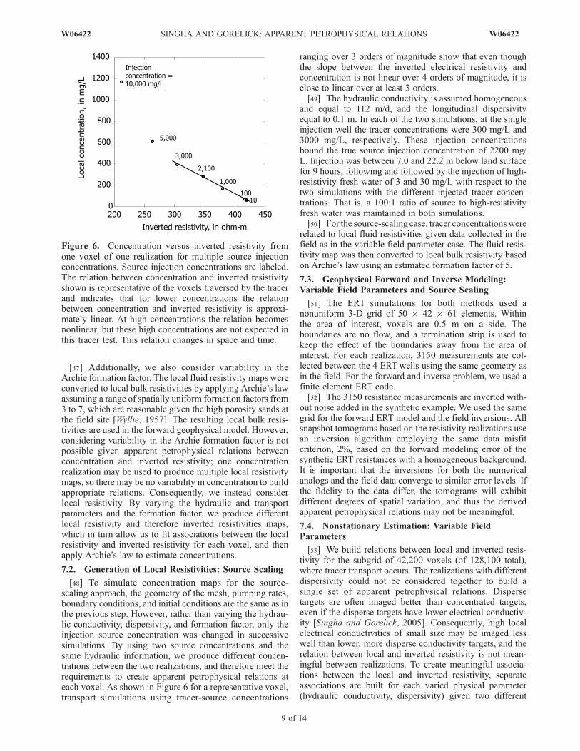
[48] To simulate concentration maps for the source-scaling approach, the geometry of the mesh, pumping rates,boundary conditions, and initial conditions are the same as inthe previous step. However, rather than varying the hydrau-lic conductivity, dispersivity, and formation factor, only theinjection source concentration was changed in successivesimulations. By using two source concentrations and thesame hydraulic information, we produce different concen-trations between the two realizations, and therefore meet therequirements to create apparent petrophysical relations ateach voxel. As shown in Figure 6 for a representative voxel,transport simulations using tracer-source concentrations

ranging over 3 orders of magnitude show that even thoughthe slope between the inverted electrical resistivity andconcentration is not linear over 4 orders of magnitude, it isclose to linear over at least 3 orders.[49] The hydraulic conductivity is assumed homogeneous

and equal to 112 m/d, and the longitudinal dispersivityequal to 0.1 m. In each of the two simulations, at the singleinjection well the tracer concentrations were 300 mg/L and3000 mg/L, respectively. These injection concentrationsbound the true source injection concentration of 2200 mg/L. Injection was between 7.0 and 22.2 m below land surfacefor 9 hours, following and followed by the injection of high-resistivity fresh water of 3 and 30 mg/L with respect to thetwo simulations with the different injected tracer concen-trations. That is, a 100:1 ratio of source to high-resistivityfresh water was maintained in both simulations.[50] For the source-scaling case, tracer concentrationswere

related to local fluid resistivities given data collected in thefield as in the variable field parameter case. The fluid resis-tivity map was then converted to local bulk resistivity basedon Archie’s law using an estimated formation factor of 5.

7.3. Geophysical Forward and Inverse Modeling:Variable Field Parameters and Source Scaling

[51] The ERT simulations for both methods used anonuniform 3-D grid of 50 � 42 � 61 elements. Withinthe area of interest, voxels are 0.5 m on a side. Theboundaries are no flow, and a termination strip is used tokeep the effect of the boundaries away from the area ofinterest. For each realization, 3150 measurements are col-lected between the 4 ERT wells using the same geometry asin the field. For the forward and inverse problem, we used afinite element ERT code.[52] The 3150 resistance measurements are inverted with-

out noise added in the synthetic example. We used the samegrid for the forward ERT model and the field inversions. Allsnapshot tomograms based on the resistivity realizations usean inversion algorithm employing the same data misfitcriterion, 2%, based on the forward modeling error of thesynthetic ERT resistances with a homogeneous background.It is important that the inversions for both the numericalanalogs and the field data converge to similar error levels. Ifthe fidelity to the data differ, the tomograms will exhibitdifferent degrees of spatial variation, and thus the derivedapparent petrophysical relations may not be meaningful.

7.4. Nonstationary Estimation: Variable FieldParameters

[53] We build relations between local and inverted resis-tivity for the subgrid of 42,200 voxels (of 128,100 total),where tracer transport occurs. The realizations with differentdispersivity could not be considered together to build asingle set of apparent petrophysical relations. Dispersetargets are often imaged better than concentrated targets,even if the disperse targets have lower electrical conductiv-ity [Singha and Gorelick, 2005]. Consequently, high localelectrical conductivities of small size may be imaged lesswell than lower, more disperse conductivity targets, and therelation between local and inverted resistivity is not mean-ingful between realizations. To create meaningful associa-tions between the local and inverted resistivity, separateassociations are built for each varied physical parameter(hydraulic conductivity, dispersivity) given two different

Figure 6. Concentration versus inverted resistivity fromone voxel of one realization for multiple source injectionconcentrations. Source injection concentrations are labeled.The relation between concentration and inverted resistivityshown is representative of the voxels traversed by the tracerand indicates that for lower concentrations the relationbetween concentration and inverted resistivity is approxi-mately linear. At high concentrations the relation becomesnonlinear, but these high concentrations are not expected inthis tracer test. This relation changes in space and time.


9 of 14

W06422

assumed formation factors. These associations were thenused in conjunction with Archie’s law generate apparentpetrophysical relations, which are then used to produce aseries of plausible concentration maps from the field ERTtomograms. Given multiple associations, multiple localresistivity maps and therefore concentration maps are esti-mated, and we plot these as plausible bounds rather thanmerely showing an estimate of the mean, which is notrepresentative of any system. Each voxel therefore has aseries of local-inverted resistivity associations, each with aunique slope and intercept, that was used to convert theinverted resistivity to estimates of local resistivities in thatvoxel. Estimates of local resistivity are then converted toconcentrations through Archie’s law.

7.5. Nonstationary Estimation: Source Scaling

[54] For the source-scaling approach, apparent petrophys-ical relations are built at every voxel given the two concen-tration realizations. Inspection of the best fit slope andintercept of the relations is instructive (Figure 7). As de-scribed earlier, in areas of poor ERT sensitivity, the slopesapproach zero, indicating that the inverted resistivities inthose locations are nearly the same for all realizations,regardless of the local concentrations. Consequently, theERT inversions are not capturing the concentration informa-tion in the areas of large slopes as well as in other parts of thetomogram. These slopes and intercepts, which make up theapparent petrophysical relations between local concentrationand inverted resistivity, are then applied to the field ERTtomograms to estimate spatially exhaustive concentration.

8. Results 2: Field Application

[55] For the field data, we use the apparent petrophysicalrelations (or the association between local and invertedresistivity used with Archie’s law) to convert the fieldtomogram for each snapshot into estimated concentrations.We compare the concentrations from nonstationary estima-

tion to concentrations estimated from direct application ofArchie’s law to the tomograms for the six time steps: 4, 5, 6,7, 10, and 12 days after injection. We then calculated thetracer mass in each case.[56] To better detect the tracer in the geophysical images,

we remove the effects of background resistivity associatedwith spatially variable fluid resistivity by differencing thepostinjection from preinjection tomograms. Although it isoften preferred to difference the data prior to inversionrather than differencing the tomograms postinversion [Dailyand Owen, 1991; LaBrecque and Yang, 2000], we saw onlyminor differences between the results of the two methodsfor the examples considered here.

8.1. Comparison Between Archie’s Law–Estimatedand Field Site Concentrations: Variable FieldParameters and Source Scaling

[57] Figure 8 shows concentration profiles at the multi-level sampler at the six snap shots. The range of concen-trations collected at the multilevel sampler over the 6-hourwindow during ERT data collection is shown in grey.Concentrations based on the simple conversion of ERTtomograms using direct application of Archie’s law consid-ering a range of plausible formation factors compare poorlyto those measured at the multilevel sampler during the tracertest. As in the synthetic case, the concentrations estimateddirectly from the ERT inversion using Archie’s law are lowcompared to the measured concentrations. The peak con-centration estimated from the ERT is often an order ofmagnitude less than that measured in the field at themultilevel sampler. However, the concentration measure-ments at the multilevel sampler indicate that most of thechanges in concentration are occurring in the top 20 m ofthe aquifer, consistent with the results of the field ERTinversions; although the tracer is visible in the differencedinversions down to 15 m, the largest changes occur above10 m (Figure 9). Although the center of mass from theArchie-estimated concentrations appears to be reasonable,

Figure 7. Slices through 3-D slope maps from apparent petrophysical relations after application ofArchie’s law for one time step using the source-scaling method. All distances are in meters. High slopeindicates an area where the concentration is high in the given realizations but the inverted resistivity mapsare not indicative of its presence. Low slope indicates areas where the relation between the concentrationand inverted resistivity is weak. The slopes are related in part to spatiotemporally varying sensitivity.

10 of 14


the values are not; this is a function of the inability of ERTto see targets far from the electrodes combined with over-parameterization of the inverse problem and the spatiallyvariable effect of regularization. The mass estimated fromdirectly applying Archie’s law to tomograms is also too low(Figure 10).

8.2. Comparison Between Nonstationary Estimatedand Field Site Concentrations: Variable FieldParameters

[58] We compare the concentration maps for each snap-shot from nonstationary estimation to field concentrationmeasurements. For the first four times, days 4, 5, 6 and 7after tracer injection, when the tracer peak is approximatelycentered over the multilevel sampler, we find that the rangeof concentration estimates using nonstationary estimationcompares more favorably to the field measurements at themultilevel sampler (Figure 8) than either those estimateddirectly from the tomogram using Archie’s law or from themean of the realizations given the range of plausible forma-tion factors. For these first four times, nonstationary estima-tion produces qualitatively reasonable concentrations overthe 3-D volume in both shape and magnitude given theknown injection concentration profile (Figures 9 and 11).The nonstationary estimation shows greater concentration atshallow depth, as seen in the injection profile.[59] We have limited concentration data at late times (days

10 and 12) to evaluate the improvement of the nonstationaryestimation compared to the direct application of Archie’slaw. Even on days 10 and 12, where very little tracer passesthe multilevel sampler, nonstationary estimation concentra-tions match the measured values at the multilevel sampler.Concentrations were also measured at the pumping well. Themeasured concentration over the fully screened pumpingwell at day 10 is 81 mg/L, while the value from nonstation-ary estimation ranges between 37 and 119 mg/L, dependingon the formation factor assumed. The mean value, however,is 78 mg/L, which closely matches the measured concentra-tion. For day 12, we see a similarly wide range: 36 mg/L to88 mg/L. The mean value, 62 mg/L, is similar to the field-measured concentration of 70 mg/L. Tracer masses estimatedusing this method have a wide range, as suggested by thewide range in concentrations. Figure 9 shows that the meanover the field site of the nonstationary estimated concen-trations is higher and the shape of the plume more reasonablethan both the direct application of Archie’s law to thetomogram or than the mean of the concentration realizations.[60] The shape of the estimated solute plume at the

multilevel sampler does not perfectly match those measuredin the field. This effect is partly an issue of scale; the ERTcannot match the detail measured in the multilevel sampler.Additionally, rate-limited mass transfer provides an expla-nation for the difference between the nonstationary estimatesand the multilevel sampler concentration: ERT is sensitive toboth mobile tracer and nonmobile tracer in dead-end pores,whereas the multilevel sampler only measures the mobiletracer. Also, the multilevel sampler concentration data arecollected in 1.6 m intervals and every two hours, so it ispossible that groundwater with higher concentrations atshallow depths was missed with direct sampling, while stillaffecting the resultant ERT inversions. We additionally arecomparing concentration measurements at one location in x-y space, a mismatch in timing in the simulations used for

Figure 8. Concentration profiles from multilevel samplerlocation. (left) Values estimated given variable fieldparameters (and shown as ranges); (right) values using thesource-scaling method. Measured field data are shown ingray, with the minimum and maximum values measuredover the 6-hour ERT data collection shown in the range. Theblue values are the Archie-estimated concentration fromthe voxels surrounding the multilevel sampler location inthe inverted field ERT tomogram. The red values are theconcentration profile from nonstationary estimation, whichin all cases, provides a better estimate of the multilevelconcentration profile measured in the field. Green is themean of the concentration realizations used to build theapparent petrophysical relations; similarity between the redand green lines indicates little improvement with nonsta-tionary estimation with respect to the assumed hydrogeo-logic information.


11 of 14

W06422

nonstationary estimation by as little as one voxel will changehow well the nonstationary estimates match the hard data. Aweighted average of neighboring cells may be a moreappropriate metric for comparison. Overall, however, non-stationary estimation allows the ERT to do a reasonable jobof replicating average tracer concentration profiles measuredin the field.[61] If the concentration realizations used to build the

apparent petrophysical relations are not representative of theaverage behavior of the tracer plume, then there will belimited if any improvement in the results. In cases whereentirely incorrect models of the subsurface geology areconsidered, nonstationary estimation may produce poorresults. Despite this, some knowledge of the field conditionsin which we work should be known, and uncertainty can beconsidered through the multiple realization approach de-scribed here.

8.3. Comparison Between Nonstationary Estimatedand Field Concentrations: Source Scaling

[62] Nonstationary estimation based on source scaling alsoproduced a better match to field concentrations than thoseestimated directly from the tomogram after applying Archie’s

law. The estimated concentrations generally lie between themaximum and minimum concentration measurements col-lected at the multilevel sampler over the 6-hour ERT datacollection window (Figure 8). The results using sourcescalingmimic the best case from the unknown field parametermethod discussed in the last section. In general, the magni-tude and shape of the concentration profiles match well;however, small-scale variability in the multilevel samplerconcentrations seen in the field data remain uncaptured.[63] The measured concentration over the fully screened

pumping well at day 10 is 81 mg/L, while the value fromnonstationary estimation provides a value of 49 mg/L;clearly this is a poor fit. However, for day 12, both the trueand nonstationary values are 70 mg/L. For day 12, theimprovement using nonstationary estimation is more signif-icant. The estimated concentrations from the source-scalingmethod are higher and more focused than those seen fromnonstationary estimation using unknown field parameters, ascan be seen in Figure 9, but the mismatch in the timing due tofixed estimates for dispersivity, hydraulic conductivity, andeffective porosity has a greater impact in the results. Despitethis problem, the field inversions show that tracer mass isbetter predicted when nonstationary estimation is employed

Figure 9. Selected slices of 3-D concentrations from three time steps (days 4, 6, and 10 after tracerinjection) estimated from (a-c) the field ERT using Archie’s law, (d-f) the concentration map estimatedfrom the mean of the realizations used in the nonstationary estimation using variable field parameters, (g-i) the concentration magnitudes from nonstationary estimation using variable field parameters, (j-l) theconcentration map estimated from the mean of the realizations used in the nonstationary estimation usingconcentration scaling, and (m-o) the concentration magnitudes from nonstationary estimation usingconcentration scaling. Concentration maps in the center are estimated given variable field parameters (themean value is shown), whereas maps on the right use the source-scaling method. All distances are inmeters. Note that the color bar changes between examples so changes in concentration can be seen.

12 of 14


(Figure 10), and the nonstationary estimates match the actualtracer mass in the system.

9. Discussion and Conclusions

[64] We have presented a method to better estimatetracer concentrations and mass from 3-D field ERT datathan traditional methods employing empirical petrophysi-cal models or site specific correlations developed fromcolocated data. Using process-based models of fluid flow,solute transport, and electrical flow, our nonstationaryestimation approach generates apparent petrophysical rela-tions between concentration and inverted resistivity. This

nonstationary estimation approach also allows us to inte-grate our knowledge of local hydrogeology and the effectsof spatial variability in the tomogram within an approachthat compensates for inversion artifacts and the sensitivityof ERT measurement. Using nonstationary estimation, weare better able to quantify tracer concentrations from ERT,as shown here in both 3-D synthetics and a field example.[65] Apparent petrophysical relations are built at each

voxel location for each snapshot, and provide a means toquantify the spatially variable resolution required forestimation of concentrations based on ERT data. Nonsta-tionary estimation is superior to direct estimation methodsthat use ERT and the simple application of Archie’s law.The approach exploits complementary information aboutthe concentrations contained in imaging provided bygeophysical data and underlying hydrogeologic processesreflected in transport modeling results.[66] Nonstationary estimation is not a cure-all for the

difficulties inherent in estimating concentrations based onelectrical tomographic inversions. Improvement providedby nonstationary concentration estimation relative to thedirect application of Archie’s law depends on a number offactors, including (1) the sensitivity of ERT data to theinverted resistivity parameters and (2) the appropriatenessof the realizations used in the simulations with respect to thefield site hydrogeology. In cases where the geophysicalinformation from ERT is noninformative, nonstationaryestimation cannot improve the concentration estimates be-yond that given by transport simulation alone. Consequently,when the tracer plume is away from the electrodes and notoptimally located for detection using ERT, the geophysicaldata may hold limited information; although nonstationaryestimation will account for spatially variable resolution, itcannot improve the information content of the geophysicaldata themselves. Additionally, nonstationary estimation willperform no better than information provided to it. Poorestimates of field site hydrogeology, in this case with respectto the average groundwater velocity as dictated by thehydraulic conductivity and effective porosity, may lead toinaccuracies in the location tracer plume and the magnitude

Figure 10. True tracer mass in the subsurface calculatedfrom the injected and pumped tracer concentrations andpumping rates compared to tracer mass estimated from(1) Archie’s law applied to field ERT tomograms and(2) nonstationary estimation through time. Values areestimated from the source-scaling method. Wide boundsexist for the variable field parameter case, although themean is similar to the source-scaling method. Nonstationaryestimation allows for a better calculation of tracer mass thanthe traditional application of Archie’s law.

Figure 11. Bulk electrical conductivity measured from (a) electromagnetic induction logs and (b) fluidelectrical conductivity measured from fluid samples. Data collected prior to tracer injection are shown inblack, after the 9-hour injection are shown in dark gray, and 24 hours after injection (electromagneticinduction log only) are shown in light gray. Tracer injection line went to 22.2 m below land surface.


13 of 14

W06422

of solute concentrations, and may affect our ability to matchdata at sampling points, such as those at the multilevelsampler and pumping well shown in our examples.[67] A strength of the method is its ability to consider

variability as shown in the field case where the field param-eters are considered unknown. As little or as much variabilityas desired can be integrated into the framework. However,there is a point where the variability of the realizations usedfor nonstationary estimation may become so large that thesubsequent concentration estimates may be difficult to inter-pret. The source-scaling method provides an alternative toestimating concentrations from tomograms. This approachprovides a means for quantifying the spatially variable ERTresolution with distance from the electrodes using fewerrealizations, and a method for estimating concentrations infield scenarios where the source concentration is unknown.[68] Nonstationary estimation provides a method for

(1) going beyond available colocated data at boreholes todevelop empirical relations between geophysical estimates;and (2) using hydrologic insight to improve the translation ofgeophysical results to hydrologic estimates. This is done byconstraining our empirical relations to be consistent with(1) a model of spatial variability, (2) hard data at boreholes,and (3) the physics of flow and transport. While we notelimitations of this method, the development of simplerelations between local and inverted resistivities providesgood results of estimated concentration. This approach is apractical alternative to joint inversion of all available data,which would achieve similar results but would be computa-tionally expensive for 4D ERT.

[69] Acknowledgments. The authors wish to thank Andrew Binley ofLancaster University for use and instruction on use of his ERT inversioncode. The advice and assistance for the field portion of this work of DenisLeBlanc, Kathy Hess, John W. Lane Jr., and Carole Johnson of the U.S.Geological Survey and the support of the USGS Toxic Substances Hydrol-ogy Program are gratefully acknowledged. This material is based uponwork supported by the National Science Foundation under grant EAR-0124262. Any opinions, findings, and conclusions or recommendationsexpressed in this material are those of the authors and do not necessarilyreflect the views of the National Science Foundation.

ReferencesArchie, G. E. (1942), The electrical resistivity log as an aid in determiningsome reservoir characteristics, Trans. Am. Inst. Min. Metall. Pet. Eng.,146, 54–62.

Binley, A., A. Ramirez, and W. Daily (1995), Regularised image recon-struction of noisy electrical resistance tomography data, paper presentedat the 4th Workshop of the European Concerted Action on ProcessTomography, Bergen, Norway.

Binley, A., G. Cassiani, R. Middleton, and P. Winship (2002), Vadose zoneflow model parameterisation using cross-borehole radar and resistivityimaging, J. Hydrol., 267, 147–159.

Constable, S. C., R. L. Parker, and C. G. Constable (1987), Occam’s in-version: A practical algorithm for generating smooth models from elec-tromagnetic sounding data, Geophysics, 52, 289–300.

Daily, W., and E. Owen (1991), Cross-borehole resistivity tomography,Geophysics, 56, 1228–1235.

Day-Lewis, F. D., K. Singha, and A. M. Binley (2005), Applying petro-physical models to radar traveltime and electrical-resistivity tomograms:Resolution-dependent limitations, J. Geophys. Res., 110, B08206,doi:10.1029/2004JB003569.

de Groot-Hedlin, C., and S. Constable (1990), Occam’s inversion to gen-erate smooth, two-dimensional models from magnetotelluric data, Geo-physics, 55, 1613–1624.

Deutsch, C. V., and A. G. Journel (1992), GSLIB: Geostatistical SoftwareLibrary and User’s Guide, 369 pp., Oxford Univ. Press, New York.

Harbaugh, A. W., and M. G. McDonald (1996), User’s documentation forMODFLOW-96, an update to the U.S. Geological Survey Modular finite-

difference ground-water flow model, U.S. Geol. Surv. Open File Rep.,96-485, 56 pp.

Hess, K. M., S. H. Wolf, and M. A. Celia (1992), Large-scale naturalgradient tracer test in sand and gravel, Cape Cod, Massachusetts: 3.Hydraulic conductivity variability and calculated macrodispersivities,Water Resour. Res., 28(8), 2011–2027.

Keller, G. V., and F. C. Frischknecht (1966), Electrical Methods in Geo-physical Prospecting, 523 pp., Elsevier, New York.

Kemna, A., J. Vanderborght, B. Kulessa, and H. Vereecken (2002), Imagingand characterisation of subsurface solute transport using electrical resis-tivity tomography (ERT) and equivalent transport models, J. Hydrol.,267, 125–146.

LaBrecque, D. J., and X. Yang (2000), Difference inversion of ERT data:A fast inversion method for 3-D in-situ monitoring, paper presented atSymposium on the Application of Geophysics to Engineering and En-vironmental Problems (SAGEEP), Environ. and Eng. Geophys. Soc.,Arlington, Va.

LaBrecque, D. J., M. Miletto, W. Daily, A. Ramirez, and E. Owen (1996),The effects of noise on Occam’s inversion of resistivity tomography data,Geophysics, 61, 538–548.

LeBlanc, D. R., S. P. Garabedian, K. M. Hess, L. W. Gelhar, R. D. Quadri,K. G. Stollenwerk, and W. W. Wood (1991), Large-scale natural gradienttracer test in sand and gravel, Cape Cod, Massachusetts: 1. Experimentaldesign and observed tracer movement, Water Resour. Res., 27(5), 895–910.

LeBlanc, D. R., K. M. Hess, D. B. Kent, R. L. Smith, L. B. Barber, K. G.Stollenwerk, and K. W. Campo (1999), Natural restoration of a sewageplume in a sand and gravel aquifer, Cape Cod, Massachusetts, U.S. Geol.Surv. Water Resour. Invest. Rep., 99–4018C, 245–259.

Moysey, S., K. Singha, and R. Knight (2005), A framework for inferringfield-scale rock physics relationships through numerical simulation, Geo-phys. Res. Lett., 32, L08304, doi:10.1029/2004GL022152.

Ramirez, A. L., J. J. Nitao, W. G. Hanley, R. Aines, R. E. Glaser, S. K.Sengupta, K. M. Dyer, T. L. Hickling, and W. D. Daily (2005), Stochasticinversion of electrical resistivity changes using a Markov chain MonteCarlo approach, J. Geophys. Res., 110, B02101, doi:10.1029/2004JB003449.

Singha, K., and S. M. Gorelick (2005), Saline tracer visualized with elec-trical resistivity tomography: Field scale moment analysis, Water Resour.Res., 41, W05023, doi:10.1029/2004WR003460.

Singha, K., and S. M. Gorelick (2006), Effects of spatially variable resolu-tion on field-scale estimates of tracer concentration from electrical inver-

sions using Archie’s law, Geophysics, 71(3), G83–G91.Singha, K., and S. Moysey (2005), Accounting for spatially variable reso-lution in electrical resistivity tomography through field-scale rock phy-sics relations, Geophysics, in press.

Slater, L., A. M. Binley, W. Daily, and R. Johnson (2000), Cross-holeelectrical imaging of a controlled saline tracer injection, J. Appl. Geo-phys., 44(2–3), 85–102.

Slater, L., A. Binley, R. Versteeg, G. Cassiani, R. Birken, and S. Sandberg(2002), A 3D ERT study of solute transport in a large experimental tank,J. Appl. Geophys., 49, 211–229.

Tripp, A. C., G. W. Hohmann, and C. M. Swift Jr. (1984), Two-dimensionalresistivity inversion, Geophysics, 49(10), 1708–1717.

Vanderborght, J., A. Kemna, H. Hardelauf, and H. Vereecken (2005), Po-tential of electrical resistivity tomography to infer aquifer transport char-acteristics from tracer studies: A synthetic case study, Water Resour. Res.,41, W06013, doi:10.1029/2004WR003774.

Wyllie, M. R. J. (1957), The Fundamentals of Electric Log Interpretation,155 pp., Elsevier, New York.

Yeh, T. C. J., S. Liu, R. J. Glass, K. Baker, J. R. Brainard, D. L. Alumbaugh,and D. LaBrecque (2002), A geostatistically based inverse model forelectrical resistivity surveys and its applications to vadose zone hydrol-ogy, Water Resour. Res., 38(12), 1278, doi:10.1029/2001WR001204.

Zheng, C., and P. P. Wang (1999), MT3DMS: A modular three-dimensionalmultispecies model for simulation of advection, dispersion and chemicalreactions of contaminants in groundwater systems: Documentation anduser’s guide, Contract Rep. SERDP-99–1, 202 pp., U.S. Army Eng. Res.and Dev. Cent., Vicksburg, Miss.

��S. M. Gorelick, Department of Geological and Environmental Sciences,

Stanford University, Stanford, CA 94305, USA.K. Singha, Department of Geosciences, 311 Deike Building, Pennsylva-

nia State University, University Park, PA 16802, USA. ([email protected])

14 of 14


hydrogeophysical tracking of three&dimensional tracer

Documents