hydrological modeling for the regional stormwater
TRANSCRIPT

HYDROLOGICAL MODELING FOR THE REGIONAL STORMWATER MANAGEMENT PLAN: AN APPLICATION AND
INTERCOMPARISON OF EVENT BASED RUNOFF GENERATION IN AN URBAN CATCHMENT USING EMPIRICAL, LUMPED VS.
PHYSICAL, DISTRIBUTED PARAMETER MODELING by
SANDRA M. GOODROW
A Dissertation submitted to the
Graduate School-New Brunswick
Rutgers, The State University of New Jersey
In partial fulfillment of the requirements
For the degree of
Doctor of Philosophy
Graduate Program in Environmental Science
Written under the direction of
Dr. Christopher Uchrin
And approved by
____________________________________________
_____________________________________________
_____________________________________________
______________________________________________
New Brunswick, New Jersey
May 2009
ii
ABSTRACT OF THE DISSERTATION
Hydrological Modeling for the Regional Stormwater
Management Plan:
An application and intercomparison of event based runoff generation in an
urban catchment using empirical, lumped vs. physical, distributed parameter
modeling
by SANDRA M. GOODROW
Dissertation Director: Christopher Uchrin
Hydrologic modeling for the characterization of two Regional Storm water Management
Plans is perform ed using both a lum ped parameter, empirical m odel and a f ully
distributed, physical m odel. Both urban/subu rban watersheds located in the Northeast
United States contain im paired waters, im pervious surfaces ranging from 15 to 25% of
total land area and are officially un-gauged. Event based models perform ed on storms
that range f rom 0.5 to 1.25 inches total dept h were m odeled to com pare the resultant
simulation hydrographs of the HEC- HMS model to the MIK E-SHE model. The results
of the calib rated model predictions compared well with the observed s tream flow in the
lumped parameter model, but were less accurate in simulating soil infiltration parameters

iii
and impervious surfaces in the fully distributed model. Sensitivity analysis of the lumped
parameter model indicated that the em pirical param eter repres enting infiltration and
runoff had the greatest effect on the accuracy of the event hydrograph . The param eter
that m ost affected accu rate sim ulation of the overland flow in the fully d istributed,
physical m odel was the land roughness coefficient, Manning M. W hen the im pervious
surfaces and unsaturated zone were included in the fully distributed model, the hydraulic
conductivity became the principal element of calibration.

iv
Table of Contents
ABSTRACT........................................................................................................................ ii 1. Introduction..................................................................................................................... 1 2. Literature Review............................................................................................................ 5
2.1 Use of Distributed Models in Watershed Planning................................................... 5 2.1.1 Defining the lumped and distributed parameter model...................................... 5 2.1.2 The application of distributed models................................................................ 8 2.1.3 Physical vs. Empirical data use........................................................................ 17
2.2 Modeling and the Regional Stormwater Management Plan ................................... 18 2.2.1 Event Based Modeling..................................................................................... 19 2.2.2 Urban Concerns ............................................................................................... 20
2.3 Review Summary.................................................................................................... 22 2.4 Purpose of this research .......................................................................................... 23
3. Methods......................................................................................................................... 24 3.1 Modeling for the Regional Stormwater Management Plan .................................... 24 3.2 Governing Equations .............................................................................................. 25
3.2.1 Empirical, Lumped Parameter Model: HEC-HMS.......................................... 26 3.2.2 Physical, Distributed Parameter Model: MIKE SHE ...................................... 33 3.2.3 Calibration Optimization ................................................................................. 42
3.3 Model Set Up: Case Studies ................................................................................... 44 3.3.1 GIS Input Data ................................................................................................. 45 3.3.2 The Pompeston Creek Watershed.................................................................... 47 3.3.3 The Troy Brook Watershed ............................................................................. 65
3.4 Planning .................................................................................................................. 78 4. Results........................................................................................................................... 80
4.1 Pompeston Creek Watershed Case Study ............................................................... 80 4.1.1 Lumped/Empirical Calibration ........................................................................ 81 4.1.2 Lumped/Empirical Validation ......................................................................... 84 4.1.3 Mount Holly Precipitation Data Set................................................................. 85 4.1.4 Lumped/Empirical Sensitivity ......................................................................... 87 4.1.4 Distributed/Physical Calibration: Method A ................................................... 89 4.1.5 Distributed/Physical Validation: Method A..................................................... 92 4.1.6 Distributed/Physical Sensitivity: Method A .................................................... 92 4.1.7 Distributed/Physical Alternative Method: Method B ...................................... 95 4.1.8 Distributed/Physical Sensitivity: Method B .................................................... 98 4.1.9 Distributed Method: Method B1.................................................................... 100
4.2 Troy Brook Watershed Case Study....................................................................... 101 4.2.1 Lumped/Empirical Calibration ...................................................................... 101 4.2.2 Lumped/Empirical Validation ....................................................................... 102 4.2.3 Distributed/Physical Calibration.................................................................... 103 4.2.4 Distributed/Physical Validation..................................................................... 105
4.3 Application and Spatial Representation of Watershed Characteristics for Regional Stormwater Management Planning............................................................................. 106
5. Discussion ................................................................................................................... 109 6. Conclusions and Recommendations ........................................................................... 127

v
References....................................................................................................................... 132
Table of Figures Figure 1: Model Sensitivity to Peaking Coefficient ......................................................... 31 Figure 2: New Jersey Case Study Watersheds.................................................................. 45 Figure 3: The Pompeston Creek Watershed Study Area .................................................. 48 Figure 4: Pompeston Creek Soil Series ............................................................................ 50 Figure 5: Pompeston Creek Soil Hydrologic Groups ....................................................... 52 Figure 6: Rating Curve for the Pompeston Creek Watershed........................................... 55 Figure 7: Pompeston Creek Input Manning M values ...................................................... 60 Figure 8: Pompeston Creek Impervious Area................................................................... 64 Figure 9: The Troy Brook Watershed Study Area............................................................ 66 Figure 10: Dominant Soil Series in the Troy Brook Watershed....................................... 69 Figure 11: Troy Brook Percent Impervious Surface Per Area.......................................... 71 Figure 12: Troy Brook Rating Curve................................................................................ 73 Figure 13: Troy Brook Manning M values ....................................................................... 77 Figure 14: Pompeston Creek HEC-HMS Calibration: 11/16/ 2005 ................................. 82 Figure 15: Pompeston Creek HEC-HMS Validation: 10/24/ 2005 .................................. 85 Figure 16: Pompeston Creek HEC-HMS alternate precipitation data for calibration ...... 86 Figure 17: Pompeston Creek Alternate Precipitation Data for Validation ....................... 87 Figure 18: Curve Number Sensitivity ............................................................................... 88 Figure 19: Intial Abstraction Sensitivity........................................................................... 88 Figure 20: Snyder Lag Time Sensitivity........................................................................... 88 Figure 21: Peaking Coefficient Sensitivity ....................................................................... 89 Figure 22: November 16, 2005 Distributed hydrograph................................................... 91 Figure 23: October 24, 2005 Pompeston Creek Watershed Distributed Method A validation Run................................................................................................................... 92 Figure 24: 10% decrease in Manning M........................................................................... 93 Figure 25: 20% decrease in Manning M........................................................................... 93 Figure 26: 10% increase in Manning M ........................................................................... 94 Figure 27: 20% increase in Manning M ........................................................................... 94 Figure 28: Manning M Sensitivity in Method A .............................................................. 95 Figure 29: Pompeston Creek Distributed Hydraulic Conductivity................................... 97 Figure 30: November 16, 2005 Pompeston Hydrograph: Method B Distributed Model . 97 Figure 31: October 24, 2005 Pompeston Method B Distributed Model........................... 98 Figure 32: Sensitivity of the Pompeston MIKE-SHE model to alterations in the hydraulic conductivity parameter...................................................................................................... 98 Figure 33: Hydraulic conductivity sensitivity hydrographs using Pompeston Creek calibration simulation of 11/16/05. ................................................................................... 99 Figure 34: Pompeston Creek October 25, 2005 Method B1........................................... 100 Figure 35: Troy Brook HMS February 1, 2008 Calibration ........................................... 102 Figure 36: Troy Brook HEC-HMS March 4, 2008 Validation....................................... 103 Figure 37: February 1, 2008 Precipitation ...................................................................... 104 Figure 38 : Troy Brook February 1, 2008 Distributed model calibration....................... 104 Figure 40: Troy Brook Precipitation March 4, 2008 ...................................................... 105 Figure 41: Troy Brook Distributed Model March 4, 2008 Validation ........................... 105

vi
Figure 42: MIKE-SHE Representation of Topography.................................................. 107
Table of Tables Table 1: Curve Numbers for unique combinations in study watersheds .......................... 29 Table 2: Applied Manning Values.................................................................................... 37 Table 3: NJDEP 2002 Land Use Data for Pompeston Creek Watershed ......................... 49 Table 4: Pompeston Creek Watershed Impervious Surface ............................................. 53 Table 5: Pompeston Creek Watershed Storm Events ....................................................... 54 Table 6: Pompeston HEC-HMS Original Loss Rate Input Parameters ............................ 56 Table 7: Pompeston Creek Original Transform Parameters ............................................. 57 Table 8: Original Soil Property Parameters for Unsaturated Zone Model (Method B).... 62 Table 9: Default input parameters for Saturated Zone Module ........................................ 63 Table 10: Troy Brook Land Uses 2002............................................................................. 67 Table 11: Troy Brook Impervious Area Coverage ........................................................... 70 Table 12: Troy Brook Watershed Storm Events............................................................... 72 Table 13: Troy Brook Original Transform Parameters..................................................... 75 Table 14: Design Storm Rainfall Depths .......................................................................... 79 Table 15: Parameters for Pompeston HEC-HMS ............................................................. 83 Table 16: Percent Change in Pompeston HEC-HMS Calibrated Parameter .................... 84 Table 17: Best Fit Manning's M Values ........................................................................... 90 Table 18: Troy Brook Calibration of Empirical Parameters........................................... 101 Table 19: Curve Number Alterations for Stakeholder Awareness ................................. 108 Table 20 : Model Input Comparison............................................................................... 125 Appendix A: Maps……………………………………………………………………..140
Map 1: Pompeston Creek Study Area ………………………………………….141 Map 2 Pompeston Creek 2002 Land Use……………………………………...142 Map 3: Pompeston Creek Soil Components…………………………………...143
Map 3A: Pompeston Creek Soil Hydrologic Group…………………………...144 Map 4: Pompeston Creek Impervious Area……………………………………145 Map 5: Troy Brook Study Area………………………………………………..146
Map 6: Troy Brook 2002 Land Use……………………………………………147 Map 7: Troy Brook Hydrologic Soil Components……………………………..148 Map 8: Troy Brook Impervious Surface……………………………………….149
Curriculum Vita………………………………………………………………………..150

1
1. Introduction
The creation of a regional stormwater management plan has become an option in
New Jersey intended to address stream water quality impairments, flooding and
groundwater recharge on a watershed scale. Although municipal stormwater
management plans are a mandatory requirement of the Stormwater Rules (N.J.A.C. 7:8),
the option of creating a regional plan allows the area to be evaluated on a drainage basis
and solutions to be prioritized for the entire watershed that is affected.
New Jersey has a large percentage of urban/suburban land use that affects these
three issues of water quality, water quantity and groundwater recharge. New Jersey also
has 566 municipalities that are governed by local councils. The regional plan has the
capability to unite two or more municipalities for the common purpose of solving these
issues that are created on a watershed level. To address these issues, a thorough
understanding of the hydrology of the watershed is essential.
Urban hydrology is often characterized by higher runoff rates due to higher levels
of impervious surfaces or compacted soils. The proper quantification of these and other
key parameters can assist in the modeling effort that will serve to simulate hydrologic
processes related to the urban watershed. A useful model of the urban New Jersey
watershed is expected to be able to help in identifying critical areas that contribute to
high runoff conditions that lead to flooding issues, lower water quality and a reduction of
groundwater recharge.
The volume of precipitation that becomes runoff in an urban/suburban area is
dependent on soil type, soil moisture, antecedent rainfall, land cover, impervious surfaces
and surface retention (USDA-NRCS, 1986). This runoff has the potential to add to the

2
volume in the stream if not infiltrated before it enters a direct connection to the stream.
In order to mitigate the effects of this urbanization on water quantity in streams, land use
options and stormwater best management practices (BMPs) can be used to infiltrate
stormwater runoff, helping to minimize impacts on water quantity, decrease flooding, and
promote groundwater recharge.
Urban and suburban land uses dominate New Jersey’s landscapes. These
urbanizing areas are now required by the Federal Clean Water Act to comply with non-
point source loading limits under adopted Total Maximum Daily Loads (TMDLs) and the
New Jersey Pollution Discharge Elimination Permits for their municipal separate storm
sewer systems (MS4s) (N.J.A.C. 7:14A). The determination of the water quality and
water quantity impact from these land uses is complicated by the impervious surfaces that
are scattered throughout the watershed. Many of these impervious surfaces are directly
connected to the stormwater conveyance system, contributing disproportionately to
stormwater runoff volumes from the watershed. Other surfaces are disconnected from
the stormwater conveyance systems and produce less of a water quantity and water
quality impact on local receiving waters. Together with soil infiltration capacity and
topography, the hydrologic character of urban features plays an important role in water
quality and water quantity issues. It would be beneficial to the TMDL process and to the
process of improving water quality and flooding issues to properly quantify the benefits
of promoting the infiltration of the runoff from these urban surfaces.
Although traditional stormwater conveyance is necessary in urban areas to
mitigate local flooding, smaller storm events can often be treated with low impact, non-
structural approaches. The infiltration of precipitation closest to the area that the rain

3
falls is the optimal situation for both baseflow maintenance and the reduction of flashy
stream flows that carry surface contaminants and erode stream banks. The accurate
modeling of these smaller storms will aid in detecting the characteristics that will
improve the stormwater management of the area.
Existing models that are currently used for evaluation of water quantity and
pollutant loading vary on the methods used to represent the urban landscape. The
computer models have the ability to represent the descriptive parameters of the watershed
spatially and can be grouped into a distributed format, a lumped format or a combination
of the two. Calculations within these models can rely on physical or empirical
equations. Spatially distributed models lend themselves to the use of physical
calculations due to the use of a grid based system of input parameters. These parameters
are to represent the characteristics of the urban catchment and proper quantification is
expected to affect the accuracy of volume and peak flow prediction.
Technological advances in computing and spatial data representation have
presented the opportunity to use a physically based fully distributed model for
representing the hydrologic scenarios necessary to watershed planning. These models
require the rigorous development and calibration to properly characterize their
practicality.
The goal of this research is to be to apply, analyze and compare results using two
prediction tools in two urban watersheds. The HEC-HMS hydrologic model, developed
by the Army Corps of Engineers, is a lumped parameter, empirical model as a
replacement for the HEC-1 model. The computation engine for the HEC-HMS draws on

4
over 30 years of experience with hydrologic simulation software (Hydrologic
Engineering Center, 2001).
The MIKE-SHE hydrologic model is a spatially distributed, physically based
model developed by DHI Water and Environment in 2003. An earlier version, SHE, was
developed in cooperation with the British Institute of Hydrology. MIKE-SHE has
undergone limited verification (www.integratedhydro.com/reviews.html), but has gained
attention with the ability to model the full extent of land based hydrological physical
processes with the increase in computer speed and size.

5
2. Literature Review
An overview of the use of distributed models used in planning and forecasting
efforts is presented here. A focus on the generation of runoff components and the
comparison to traditional lumped parameter models together with a concise description of
the uses of empirical versus physical models is intended.
2.1 Use of Distributed Models in Watershed Planning
The benefits of using a distributed model are the ability to represent land use
change, spatially variable inputs and outputs, pollutant and sediment movement, and
hydrological response at un-gauged sites (Beven, 1985). However, the broad use of this
tool was hampered until recently by intense data requirements and the computational
efforts that are required.
2.1.1 Defining the lumped and distributed parameter model
The distributed model is differentiated from the lumped parameter model in the
spatial aspect that the descriptive data inputs are represented. The lumped parameter
model “averages” these properties together, over a delineated area, using a weighted
approach. A distributed parameter model will allot distinctive cells, usually a measured
grid area, which will be used to calculate mass and momentum changes between cells.
The lumped parameter model generally performs calculations using empirical based
formulas, whereas a fully distributed model can employ physical calculations.
A well developed lumped parameter model using empirical representation of the
watershed characteristics is the Hydrologic Engineering Center Hydrologic Modeling

6
System (HEC-HMS). The HEC-HMS model has been developed by the United States
Army Corps of Engineers (ACOE). Evolving from the need to capture the knowledge of
WWII engineers approaching retirement age, the ACOE established a division to
organize and present water resources development activities, and out of that came the
HEC grouping of software. Early versions of the hydrologic software component date
back to the 1970’s. (http://www.hec.usace.army.mil/whoweare/history.html).
The distributed models are defined by the spatial distribution of the physical data
input and the calculation of the processes that occur in that space. A distributed model
will produce model evaluation output (i.e. infiltration depth, overland flow) at the level of
grid scale. A lumped parameter model will only produce output elements at the outlet of
the delineated sub-area. The spatial distribution of data is the key to the distributed
model, and the use of physical calculations within the spatial extent would be expected to
best represent the hydrological processes that occur in a watershed, with excess
precipitation experienced in each cell over each time step being routed to the next down-
gradient cell.
Language in the literature has developed an understanding of the components of a
distributed model, however, inconsistencies do exist. Two examples of inconsistencies of
definition are the SWAT model (USDA and Texas A&M) and the TOPmodel. The
SWAT model is considered by some to be a distributed model (Sangjun, 2007; Yang,
2008; Wang, 2008) being that there is accounting of spatial variability of land use and
other input parameters. SWAT uses the “Hydrologic Response Unit” (HRU) in
determining the parameterization of the model. These units can be adjusted for desired
size with the ability to essentially replicate the size of the grid with the delineation of

7
drainage areas or to perform calculations on subbasins. SWAT is basin scale,
continuous-time model that operates on a daily time step. In SWAT, a watershed is
divided into multiple subwatersheds, which are then subdividied into hydrologic response
units (HRU’s) that consist of homogeneous land use, management, and soil
characteristics. The HRU’s represent percentages of the subwatershed and are not
identified spatially within a SWAT simulation (Gassman, et al., 2007). Also, in SWAT,
the excess volume of runoff is routed directly to the stream, with no ability for this water
to pass over the land of the next “cell”. This is performed with the assumption that since
the lag time would be less than the model time step, that this excess would become part
of the stream flow in that time. This characteristic would complicate representation of
the watershed hydrology at an event scale.
TOPMODEL has been represented as being distributed and semi-distributed
(Peng, 2008; Takeuchi, 1999). An EPA fact sheet describing TOPMODEL begins by
defining it as a physically based distributed watershed model.
(http://www.epa.gov/nrmrl/pubs/600r05149/600r05149topmodel.pdf) TOPMODEL does
not account for the spatial variability of hydrological important features such as climate
and soil, but will only allow for the spatial distribution of topography (Franchini, 1996).
The TOPMODEL has rarely been applied to large areas due to the fact that it was
developed for the hillslope/catchment scale and not the drainage basin scale (Quinn et al,
1995).
It has been suggested that so-called physically based distributed models are in
reality lumped conceptual models operating at the grid scale (Smith, 2004). Carpenter
and Georgakakos (2006) of the Hydrologic Research Institute (United States Scripps

8
Institution of Oceanography, CA) differentiate the distributed and lumped parameter
model by being of “high or low spatial resolution”. The method in which excess
precipitation is routed has not been included in this definition.
For the purpose of these case studies, the HEC-HMS modeling system is
considered the lumped, empirical model using delineations of subbasins and is compared
to the MIKE-SHE model, which in using a grid scale to compute hydrologic processes is
considered the fully distributed, physical model.
2.1.2 The application of distributed models
Different types of distributed hydrological models are developed in the literature.
These models vary in their degrees of complexity and appropriateness.
In a collaborative effort to evaluate the use of distributed hydrological models as
compared to lumped parameter models, the Distributed Model Intercomparison Project
(DMIP) was initiated to “infuse new science” into the river forecasting capability of the
National Oceanic and Atmospheric Administration’s National Weather Service
(NOAA/NWS). The NWS is mandated to provide river and flash flood forecasts for the
entire US and has forecasts being generated for over 4,000 points daily. Currently, these
forecasts are being generated through the use of the lumped parameter model, the
Sacramento Soil Moisture Accounting Model (SAC-SMA), which is a 2-layer conceptual
model (Smith, 2004). The results of the varying distributed models that were employed
for this effort were all compared to the runoff components that were generated from the
SAC-SMA lumped parameter model.

9
The DMIP used data for eight basins that ranged in size from 65 to 2484 km2 (25
to 959 mi2) and simulations generally consisted of continuous (7 to 20 years) model runs
in gauged streams.
Models that were considered for inclusion in the DMIP included SWAT
(Agricultural Research Service), MIKE 11(DHI), NOAH Land Surface Model
(Environmental Modeling Center), HRCDHM, tRIBS (MIT), VIC-3L (University of
California at Berkeley), TOPNET, (a networked version of TOPMODEL)(Utah State
University), WATFLOOD (University of Waterloo, Ontario) and LL-II (Wuhan
University). The spatial units for rainfall-runoff calculations included hydrologic
response units (6-7 km2), subbasins (60-180 km2) and grids (0.02- 4 km2) (Smith, 2004).
Results of the DMIP showed that for the greatest percentage of the basin studied,
the lumped parameter models showed better overall performance (Reed, 2004).
However, some distributed models showed comparable results in many basins and some
improvements in other basins. With the dominant land use of all the basins being
agriculture, the basins were not considered urban in nature.
The goal of the DMIP was to evaluate the use of distributed precipitation
databases as they are used in distributed hydrologic models for the purpose of flood
prediction. The definition of distributed hydrologic model was not well defined, with the
spatial characteristics of the watershed represented in varying capacity.
Although many distributed models are available, it is necessary to determine the
appropriate intended use of the currently designed computer packages. The intention of
the DMIP was to evaluate precipitation. Other distributed models provide detailed
information on land based characteristics, such as topography. Several models were

10
considered for use in this comparison case study for regional stormwater management
planning, and samplings of those models considered are briefly described here. Of those
considered, TOPMODEL and MIKE SHE were also evaluated in the DMIP.
SMDR (Soil Moisture Distribution and Routing Model):
In research at Cornell University, small agricultural watersheds were modeled to
determine the optimal placement of infiltration Best Management Practices (BMPs).
Using a distributed model created at the University called the Soil Moisture Distribution
and Routing (SMDR) model, the effects of the saturation capacity of the soil were
analyzed. This tool was used to identify areas within the watershed where saturation
occurs, thus being areas that are undesirable for promoting infiltration. Researchers at
Cornell University determined that this tool which was shown to accurately predict
spatial runoff generation zones is critical to the proper placement of BMPs within the
watershed. This model was recently adapted to urban areas that include impervious
surfaces and hydraulic control structures (detention basins) (Easton, 2007). This model
was applied and validated on a 332 ha (1.28 mi2) in determining the distributed watershed
response. (Gerard-Marchant, et al., 2006 and Easton, 2007). Employing physical
parameters, efforts were made to represent variable source areas (VSAs), or areas located
near the base of high gradient change where accumulation of runoff would be expected to
saturate the area making it undesirable for the location of infiltration BMPs.
SMDR possesses a physical structure that represents well the hydrologic
characteristics of the watershed with high gradient slopes. However, the model was run
on a LINUX platform and used GRASS (Geographic Resources Analysis Support
System) for geospatial data input. The model has not been fully maintained and is not

11
readily available. Although SMDR is a public domain model, website information has not
been kept current and model support is not available.
TOPMODEL:
TOPMODEL (a TOPography based hydrological MODEL) models rainfall-runoff
in a single or in multiple subcatchments, in a “semi-distributed” way and uses gridded
elevation data for the drainage area. A conceptual model, it is often considered a
physically based model, with its parameters being able to be theoretically measured in
situ (Beven and Kirkby, 1979, Beven et al., 1984).
The development of TOPMODEL was initiated by Professor Mike Kirkby of the
School of Geography, University of Leeds under funding from the UK Natural
Environment Research Council in 1974. TOPMODEL is considered a collection of
concepts that can be used where appropriate, which would be considered catchments with
shallow soils and moderate topography which do not possess long dry periods (Young et
al., 1994).
TOPMODEL uses the spatially distributed data of the topography of a watershed
to determine the key physical input parameters of ln(a/tanβ) that describes the upslope
area and movement of water over the slope gradient. The model allows for
multidirectional flow of excess precipitation in 8 directions (Franchini et al., 1996).
Parameters such as soil characteristics and precipitation distribution are input over larger
scales and are not considered fully spatially distributed.
TOPMODEL was used to interpret the relationship of catchment topography and
soil hydraulic conductivity to lake alkalinity (Wolock et al, 1989), to evaluate the effects
of subbasin size on topographic characteristics and simulated flow paths (Wolock, 1995)

12
and was used at Princeton University where macro scale, dimensionless and fully
distributed versions were used (Sivapalan et al, 1987; Wood et al, 1988; Familglietti et
al., 1992). The use of TOPMODEL is limited due to the specific watershed
characteristics previously discussed. Although a public domain model, recent use has
been diminished due to lack of institutional support.
tRibs (TIN-based Real-time Integrated Basin Simulator):
tRibs is a distributed, physically based model licensed by MIT, based on a UNIX
platform and is not publically available. The model emphasizes the dynamic relationship
between a partially saturated vadose zone and the land surface. Initially designed to use
the grid cell as its calculation basis, the model has been developed to use the “voronoi
cell” which is adjusted to better fit the terrain.
(http://hydrology.mit.edu/index.php/Models/TRIBS). With the focus on hillslopes, the
role of topography in lateral soil moisture redistribution has been studied, with rainfall
intensity and initial groundwater position strongly influencing model output (Noto,
2008).
The tRIBS model emphasizes the relationship between the partially saturated
vadose zone and the land surface being affected by the precipitation event. This is
performed by computing the moisture fronts created in relation to the water table. Using
these operations, the model is able to produce runoff through several runoff generation
mechanisms, including infiltration excess and saturation excess. However, this excess is
currently routed to the outlet and not downgradient to the next cell (Vivoni, 2005).
Currently used primarily for research purposes, the model has been studied for its
resulting simulations involving ecohydrology, fluvial geomorphology, hydroclimatology

13
and watershed hydrology. The goal of the work in watershed hydrology is to utilize this
model as a hydrometerological forecasting system for the prediction of the spatial and
temporal response in very large basins, in the area of hundreds to thousands of square
kilometers. Current projects include the evaluation of predicting soil moisture using
multiple data sources and climate dynamics involved with the fully distributed hydrologic
model (http://hydrology.mit.edu/index.php/Research/Hydrology).
The tRIBS model is intended for research purposes and has not been
demonstrated for planning purposes of small urban watersheds. Together with the model
complexity, limited availability and UNIX platform, tRIBS does not offer the easy option
of investigation for use in planning purposes, but may in the future.
MIKE SHE (System Hydrologique European):
MIKE-SHE is a grid based distributed hydrological model developed jointly by
the Danish Hydraulic Institute (Denmark) and SOGREAH (France) (Xevi, 1997). The
MIKE SHE modeling system (Refsgaard and Storm, 1995) is a deterministic fully
distributed and physically based model which can incorporate all major processes of the
land phases in the hydrologic cycle. A finite difference approach is used to solve the
partial differential equations of overland, channel, unsaturated and saturated subsurface
flows (Thompson, 2004).
Applications of MIKE SHE include the use of the model for lowland wet
grassland (Thompson, 2004) with two consecutive eighteen month periods being used to
investigate the models abilities to represent the physical movement of water through this
type of landuse. The conclusions found sensitivities in the land topography and
macropore flow.

14
Christiaens and Feyen (2001) evaluated uncertainties associated with different
methods used to determine soil hydraulic properties using the physical calculations of the
MIKE SHE model. The four methods of obtaining soil hydraulic properties include
(i)moisture retention lab measurements, (ii) prediction via pedo-transfer functions (PTFs)
using field texture measurements, (iii) prediction via PTFs using USDA texture classes,
and (iv) prediction through the bootstrap-neural network approach using field texture
measurements, with the neural network producing the lowest uncertainties.
Vazquez et al. (2002) evaluated the effect of grid size on the performance of the
MIKE SHE code. Using a 326 km2 drainage area and daily catchment discharges and
observed water levels, the grid sizes were varied from 300, 600 and 1200 m2. It was
determined that, for the given level of data input and quality, that the 600 m grid
resolution was the most appropriate.
The calibration and validation efforts surrounding the MIKE SHE model have
taken a variety of routes. Using the Neuenkirchen Research Catchment, researchers
calibrated and validated the MIKE SHE model with a two-year time series of stream
flows at the outlet of the basin, finding that peak overland flow and total overland flow
were very sensitive to resistance parameters and to the vertical hydraulic conductivity of
the surface soil (Xevi et al., 2007). The model output variables considered were not
significantly affected by the vegetation parameters nor by the specific storage coefficient.
Using the Generalized Likelihood Uncertainty Estimation (GLUE) on a MIKE-
SHE model, McMichael et al. (2006) calibrated, and provided predictive uncertainty
estimation in monthly stream flow in a semi-arid shrub land catchment in central
California. A focus area in this study was the representation of the remote sensing-based

15
Leaf Area Index (LAI) and its use in fully distributed models. Results indicate prediction
uncertainties are generally associated with large rainfalls and wildfires.
As a part of the FLOODRELIEF project (Butts, 2005), the MIKE SHE model was
developed to provide a flexible, hydrological modeling framework that permitted both
conceptual and physics based processes to be used in a spatially explicit manner. The
model was evaluated for use in a flood prone basin for operational hydrological
forecasting so as to evaluate the trade off between model complexities and accuracy
against the needs for rapid flood forecasts. In the evaluation of two large watersheds, the
Blue River in Oklahoma and the Odra River in Poland, the spatial resolution of
precipitation distribution was observed to reach a point where increase discretization
would not increase model accuracy. It was concluded that there may be model
limitations if the purpose is to predict flows at catchment outlets. There may also have
been a limitation in one or more areas of the model: 1) the model structure itself, 2) the
available calibration data, 3) the accuracy and representation of rainfall, or 4) the
parameter estimation procedures (Butts, 2005).
The physical equations that the MIKE SHE model is based on are the equations
that have been developed as the science of hydrology has evolved. Using these equations
on a watershed scale poses several challenges to the modeler. These challenges include
the proper characterization of spatial data. Although the collection of spatial data has
improved with the use of GPS and GIS, it has not been demonstrated that using these data
on a watershed scale with these physical calculations can provide reliable simulations of
the hydrological processes.

16
Additional Distributed Models Refsgaard and Knudsen (1996) compared the complex distributed model (MIKE
SHE), a lumped conceptual model (NAM) and an intermediate complexity model
(WATBAL) on data-sparse catchments in Zimbabwe. Their results could not strongly
justify the use of the complex distributed model, although the distributed model
performed marginally better for cases where no calibration was allowed. This was the
conclusion after attempts at calibration actually produced simulations that were less
acceptable, which made proper characterization of the input parameters more important.
The three watersheds in Zimbabwe ranged in size from 98 mi2 to 421mi2 and no
characterization of impervious surfaces were included.
Refsgaard (1997) determined that distributed models calibrated to basin outlet
information did not adequately represent internal piezometric conditions. In contrast,
Michaud and Sorooshian (1994) determined that a complex distributed model was able to
simulate internal conditions at least as accurately as the outlet simulations. A comparison
of basin attributes and input data should be considered.
Reed et al. (2004) attempted to explore the connection between conceptual and
physically based models for hydrologic prediction. Using the simulations of a total basin
area of 256 km2 basin, the effect of rainfall distribution and grid size were evaluated to
determine the effects on the infiltration processes, with the infiltration excess type models
being the most sensitive to rainfall distribution.
Identified Limitations of Distributed Models
Input parameters to fully distributed hydrologic models include the spatial
discretization of land use, soil types, topography, precipitation, land cover and man made

17
hydraulic structures. The availability of this data is changing rapidly with the
improvements in satellite acquisition and computer technology. A move toward centrally
accepted data sets is taking place in order to support the collaboration of multiple users.
ESRI, a company that provides Geographic Information Systems (GIS) and mapping
software, has provided and created formats for spatial data since 1969. An alternative to
ESRI GIS is the open source software, Geographic Resources Analysis Support System
(GRASS), which is not fully supported in the United States.
The resolution of the topography, soil classifications, precipitation distribution
and other key input parameters to distributed models have been evolving. Data is
collected on the ground and digitized, paper maps are digitized into formats compatible
with GIS systems, and remote sensing data are becoming available. As thes data evolve,
distributed models improve their ability to fully represent the characteristics of the
watershed and provide useful simulations of hydrologic activities that will aid in
watershed planning efforts.
2.1.3 Physical vs. Empirical data use
Flow governing equations have developed for both empirical and physical
models. Borah (2003) provides the physical flow governing equations used in the
distributed model, MIKE SHE, as well as other physical models. Empirical models have
taken many formats, with the NRCS/TR-55 methodology presenting a simplified
procedure to calculate storm runoff volume, peak rate discharge, hydrographs and storage
volumes. The TR-55 format is applicable to small urbanizing watersheds (USDA NRCS,
1996). Equations used in this study are documented in the following section.

18
The physical parameters observed in spatial databases commonly used in GIS can
be used as descriptive data, or they can be used to determine the empirical parameter that
is generally accepted to represent the data.
Strategies for the calibration of empirical models are better defined than for
physical models. Truly “calibratable” parameters in the physical model are limited, as
physical parameters are intended to be measurable in the field or derived from field
measurements (Storm and Refsgaard, 1996). Given that parameter adjustments are used
for improved model performance, the distinction between physically based parameters
and empirical parameters become distorted.
The SWAT model, a public domain model, enjoys large support from the USDA
and Texas A&M and therefore has been able to revise code to implement modifications
necessary for optimal hydrologic processing. The MIKE-SHE model is supported by
DHI, an independent, international research and consulting firm that is globally
dispersed.
2.2 Modeling and the Regional Stormwater Management Plan
The Regional Stormwater Management Planning Process was promulgated by
New Jersey by statute in February of 2004 (36 N.J.R. 670). Although municipal
stormwater management plans became mandatory with this document, the regional plans
remained voluntary, yet recommended and well guided. The basis for this
recommendation lie in the fact that watersheds cross municipal and/or county boundaries,
yet solutions to water quality and water quantity issues should be formulated over the
area of the watershed in question.

19
The author of this text participated in the development and hydrologic modeling
of four Regional Stormwater Management Plans in New Jersey (Goodrow, 2005; RCE
WRP, 2007 (a), (b), (c)). Three of these plans, including the Troy Brook Watershed in
Morris County and the Pompeston Creek Watershed in Burlington County were accepted
by the New Jersey Department of Environmental Protection as official watershed plans.
The hydrologic modeling performed for these plans used the lumped parameter model,
HEC-HMS. The implementation of the NRCS TR-55 CN method provided valuable
information about the rainfall-runoff capabilities of the watersheds and served to aid in
the planning efforts regarding infiltration and the reduction of water quantity and quality
issues.
As planning efforts in these watersheds continue, it is desirable to evaluate
distinct land areas for their contribution to the water quality or water quantity issues. To
this end, the implementation of a spatially distributed model was undertaken.
2.2.1 Event Based Modeling
In a study of the frequency and intensity of rainfall events in the Mid-Atlantic
region, it was determined that up to ninety percent of all storm events produce less than
one inch of rain (Claytor & Schueler, 1996). These storms contribute diffuse source
pollution and flashiness to the streams to which the land drains. The correct
characterization of these storms in a hydrologic model is expected to aid in the resolution
of issues addressed in Regional Stormwater Management Plan.
Event based modeling is a common practice for semi-arid watersheds (10-20
inches of precipitation per year) where runoff is restricted to short periods after a storm

20
(Maneta, 2007). Event modeling can also be used if continuous data are not available or
if the results from specific events are required (Haiping, 1998).
A boundary condition that represents the watershed characteristics before the
storm event is necessary. In the case of the lumped parameter, empirical model, the 5-
day antecedent moisture condition is implicit in the selection of curve numbers,
according to the NRCS TR-55 method. An average antecedent moisture condition is
assigned according to the location of the watershed (USDA NRCS, 1996). The boundary
conditions for the distributed model were a “hotstart” file obtained from the modeling
scenario of a one year precipitation record taken within New Jersey. With the small
storm event greatly contributing to the stormwater issues experienced by urban/suburban
watersheds, it is essential that these storms be accurately characterized for planning
purposes.
2.2.2 Urban Concerns
The parameters used in the hydrologic models are expected to be altered due to
the effect that urbanization has on the watershed. This urbanization could take the form
of increased impervious area or soil compaction, in addition to constructed hydraulic
structures including traditional stormwater conveyance.
In a lumped parameter model, these attributes are “weight averaged” and assigned
a descriptive empirical value. This empirical value is used for the calibration purposes of
this watershed model, and is expected to be altered in poorly characterized urban areas.
In urban areas, the process of weight averaging increases uncertainty due to the level of
connected or disconnected impervious areas (Althouse, 2007).

21
Disconnected impervious area (DCIA) has disproportionately contributes to the
total runoff volume of the watershed. Lee (2003) determined that DCIA covering 44% of
the watershed contributed to 72% of the runoff volume. Increasing the accuracy of
connected versus disconnected impervious area resulted in a lower percentage of directly
connected impervious area and therefore caused reduced modeled output volume.
However, in the modeling of most planning scenarios, it is difficult to determine
the absolute amount of connected and disconnected impervious surfaces. In many
situations, a range of scenarios can be implemented to evaluate the potential effects of
alterations in the amount of connection/disconnection. In lumped parameter models this
may be performed with a calibration effort. Physical parameters are not intended to be
calibrated, and therefore need to be properly characterized as input data.
Soil attributes are similarly represented in the lumped/empirical and
distributed/physical models. Infiltration and runoff due to soil characteristics are
represented by a calibratable parameter in the HEC-HMS model, but physical properties
are necessary input to the MIKE-SHE model. Conventional soil maps use a 1:24,000
mapping scale with a minimum mapping unit of 2.5 to 5 ha (Quinn, 2005). Combined
with the unknown physical alterations due to urbanization, the physical soil attributes are
thought to vary from reported values (Rodriquez, 2008). Characteristics of urban soil can
also contribute to the flow rate in the form of subsurface flow (Berthier et al., 2004).
This further complicates the physical parameterization of the urban environment where
heterogeneous soil characteristics are present.

22
Best Management Practice Predication Tool
Stormwater management includes the proper placement of “Best Management
Practices” (BMPs) that can be used to enhance the infiltration properties of the watershed
or slow the direct addition of runoff to the receiving streams. Using a general
spreadsheet model and HRUs, the optimal location to place a BMP within a watershed
was determined to be complex function of watershed network connectivity, flow travel
time, land use, distance to channel and contributing area (Perez-Pedini, 2005). In an
urban area, the placement of any stormwater management practice is dependent on
available land area. These restrictions make the use of an accurate fully distributed
model for stormwater management planning more desirable.
2.3 Review Summary
The fully distributed physical model can play a valuable role in the planning
process and in stormwater management scenarios. A well parameterized distributed
model can provide reliable scenarios in un-gauged streams. (Refsgaard and Knudsen,
1996).
Several distributed modeling efforts have focused on continuous based modeling
or flood prediction modeling. The DMIP focused on flood forecasting for the NWS. The
distributed model can aid in the planning efforts necessary to address watershed
impairments due to diffuse source pollution that is dependent on the urban hydrology
better than the well developed lumped parameter model. To do this, small storm events
must be characterized properly.
Urban and suburban areas would benefit greatly from the use of distributed
hydrologic models, and spatial data that currently exists should be evaluated for their

23
ability to characterize the input for the physical calculations that will predict overland and
outlet flows. In urban watersheds, the spatial distribution of impervious surfaces in urban
land use and the urban nature of soils must be well differentiated.
These New Jersey watersheds do contain a range of connected and disconnected
impervious areas that are expected to affect the volume and peak flow of the resultant
hydrograph. Calibration of these models will help determine if these models can be used
to provide a basis for the adaptive management of the use of these models in future
planning efforts.
2.4 Purpose of this research
This study will apply the distributed, model, MIKE-SHE to two urban/suburban
watersheds in New Jersey, in the Northeast United States. Both of the urban watersheds
considered in this study generally have a low gradient land elevation change and
therefore are not expected to replicate the drainage that is present in variable source
areas, as was determined with studies involving the SMDR model. And with limited
distributed models being used in urban/suburban areas, this study will provide
applications for two case studies as well as an intercomparison of those models to their
lumped, empirical counterparts currently being used in planning efforts.
This study will seek to determine if the fully distributed physical model can be
utilized in a watershed planning effort with current levels of existing spatial data. A
sensitivity analysis will compare and contrast the distributed model with the lumped
parameter model and provide a guide to increasing optimal parameterization in future
scenarios, using a calibrated model and event based scenarios.

24
3. Methods
3.1 Modeling for the Regional Stormwater Management Plan
There can be several reasons for creating hydrologic models for regional
stormwater management planning. Each watershed may experience different
stormwater issues, including flooding, nonpoint source pollution, or the
degradation of the freshwater biota. The issues experienced in urban watersheds
have been related to the percent of overall impervious surface (Hatt, 2004; Lee,
2003) and the traditional methods of stormwater conveyance that routes the
stormwater quickly to the nearest stream.
Accurately predicting the overland flow and stream flow caused by the
smaller storms that dominate precipitation events is the key to protecting the
water quality of the stream. It has been observed that storms less than 0.5 inches
can be significant in the mass loading of diffuse pollution, but storms from 0.5 to
1.5 inches are thought to be responsible for most bacterial pollutant mass
discharges (Pitt, 1998).
The designation of an accurate drainage area is necessary for a stormwater
evaluation. For the initial hydrological modeling for the Regional Stormwater
Management Plans, the watershed delineation and subbasins delineation was
determined using the HEC-GeoHMS pre-processing software. This program
allowed for a subbasin delineation which could incorporate the user defined outlet
desired for each drainage area. This process permits not only the use of
knowledge regarding the land use in the watershed and stream morphology, but

25
can achieve subbasins of similar size. Algorithms within the program determined
the flow paths expected with the input of the 10-m digital elevation model (DEM)
representing the topography at a 10-m resolution. These data are available from
the New Jersey Department of Environmental Protection GIS database, using
sources originating at the USGS.
3.2 Governing Equations
The modeling for the stormwater management plan has been carried out
using two different hydrologic models. The first model, HEC-HMS, is considered
a lumped parameter, empirical model. The lumped model assumes that the
watershed can be broken down into units and described by a set of empirical
parameters that will be weight averaged over the delineated subbasins and will
ultimately define how that watershed is mathematically represented.
The second model, MIKE-SHE is considered a fully distributed, physical
model. The calculations of the hydrologic processes are determined primarily
with the use of physical equations using watershed characteristics. This is
performed on a grid level basis, with the characteristics found in each grid cell
used for calculation purposes.
Input data from Geographic Information Systems (GIS) data layers
(shapefiles) have been used in both model types. The important GIS layers that
are considered essential to regional watershed hydrologic modeling are the land
use, the soils, and the topography. These digital components of the model can
come in varying resolutions, but layers based on the 7.5 minute, 10-m X 10-m
DEM were readily available and used in this project.

26
HEC-GeoHMS was used to prepare the input shapefiles for use in the
HEC-HMS model. This preparatory function derived the necessary geometric
features (slope, length, area, centroid location) from the base topography data
input. The preprocessing of GIS data is necessary for the physical model, since
the model calculates the hydrologic output on a grid level.
3.2.1 Empirical, Lumped Parameter Model: HEC-HMS
HEC-HMS provides several options from a collection of methods to
simulate the processes of rainfall-runoff, such as infiltration losses, runoff
transform and flow routing. For the purpose of this study, the Soil Conservation
Service (SCS) Curve Number (CN) Loss Model was used to estimate the
precipitation excess and determine runoff volume from each watershed. The
Snyder unit hydrograph was used as the runoff transform method, and the
Muskingum-Cunge method was used to simulate stream flow routing. HEC-HMS
provides as a final result the hydrograph (flow vs. time plot) and peak flow for
model elements such as junctions, reaches and reservoirs.
For the purpose of modeling for this study, the next sections present the
components chosen for use in the lumped parameter, HEC-HMS model.
Basin Model Setup
HEC-GeoHMS was used to process the available digital data. The digital
input files to the HEC-GeoHMS program are the 10-m digital elevation model
(DEM) that defines the topography of the area and the stream definition shapefile.
Through the algorithms contained in the program, files were created that served as
the input for the basin model set up in the HEC-HMS model. The processing of

27
these input files allows the delineation of the watershed boundaries and subbasin
boundaries. The program also quantifies the lengths of the rivers, longest flow
paths, slopes, centroid locations and the lengths to the centroids. The basin
schematic and map file used to represent the watershed are also created here.
Runoff volume (Loss Rate)
Using the SCS Curve Number Loss Model, the precipitation excess is
determined by the following equation:
SIPIPPa
ae +−
−=
2)( Equation 1: HMS Precipitation Excess (USDA, 1986)
where Pe = accumulated precipitation excess at time (in) t; P = accumulated
rainfall depth (in) at time t; Ia = the initial abstraction (in) and S = the potential
maximum retention (in). The initial abstraction is intended to represent the
portion of rainfall that is intercepted by vegetation and is accumulated as
depression storage. The maximum retention is the quantification of the ability of
a watershed to abstract and hold storm precipitation. The empirical relationships
reported in the TR-55 manual have been determined through the study of many
agricultural watersheds. The initial abstraction is related to the potential
maximum retention (S)(in) in the watershed, which is empirically related to the
CN as in the following equations:
SIa 2.0= Equation 2: Empirical relationship of Ia and S (USDA, 1986)

28
CNCNS 101000 −
= Equation 3: Empirical relationship of S and CN (USDA, 1986)
Estimation of the Curve Number
This method employs the assignment of a “curve number” (CN) to
represent the empirical relationship that relates soil and the land cover with total
runoff volume. The curve number method has been developed by the National
Resource Conservation Service (NRCS), Technical Release 55 (USDA, 1986).
The CN ranges between zero and 100, with the higher numbers denoting the
higher runoff capabilities. Low curve numbers generally do not fall below 30,
with a soil assigned a CN of 30 being considered a permeable soil with a high
infiltration rate (HMS technical manual, p. 41).
The curve numbers that were assigned for the watersheds in this study
were derived from the CN tables in TR-55. The GIS databases containing the soil
hydrologic attribute (hydrologic group) (http://www.nj.nrcs.usda.gov/)
and the land use/land cover (NJDEP, 2002) attributes (Type 02) were joined to
produce a single GIS database that would provide individual polygons (i) which
each had the attributes necessary to assign a single value (Table 1) of a curve
number (CNi).

29
Table 1: Curve Numbers for unique combinations in study watersheds HYDROLOGIC SOIL
GROUP LAND USE A B C D Agricultural Wetlands 98 Altered Lands 76 91 94 Artificial Lakes 100 100 100 Athletic Fields (Schools) 49 69 79 84 Commercial Services 89 92 94 95 Coniferous Brush/Shrubland 94 Coniferous Forest (10-50% Crown Closure) 73 Coniferous Wooded Wetlands 98 98 Cropland and Pastureland 72 81 88 91 Deciduous Brush/Shrubland 35 56 70 77 Deciduous Forest (>50% Crown Closure 30 55 70 77 Deciduouos Forest (10-50% Crown Closure) 43 65 76 82 Deciduous Scrub/Shrub Wetlands 98 98 98 Deciduous Wooded Wetlands 98 98 98 98 Disturbed Wetlands (Modified) 98 98 98 Extractive Mining 81 88 Former Ag Wetland 98 Freshwater Tidal Marshes 98 98 98 98 Herbaceous Wetlands 98 98 98 Industrial 81 88 91 93 Managed Wetlands 98 98 Mixed Deciduous/Coniferous Brush/Shrubland 60 73 79 Mixed Forest 55 70 77 Mixed Urban or built-up land 92 94 Natural Lakes 100 100 100 Old Field (<25% Brush Covered) 48 67 77 83 Orchards/Vineyards/Nurseries/Horticultural Areas 88 91 Other Urban or Built Up Land 49 69 79 84 Recreational Land 49 69 79 84 Residential, High Density, Multiple Dwelling 77 85 90 Residential, Rural, Single Unit 46 65 77 82 Residential, Single Unit, Low Density 54 70 80 85 Residential, Single Unit, Medium Density 61 75 83 87 Transportation 69 79 84
(USDA, 1986)
These curve numbers were then area-weighted, or composited, to produce an
overall curve number for the subbasin of interest (CNcomposite) (USACOE HMS
Technical Manual, p. 41). This composite curve number is calculated as shown in
Equation 4.

30
i
iicomposite A
CNACN∑
∑=
Equation 4: Composite Curve Number (USDA, 1986)
Where Ai= area of polygon with single assigned CN (CNi).
Impervious Area
A third component of the runoff volume computed by the HEC-HMS
model is the percent impervious area. Although there is an available option to
denote this element separate from the assigned curve number, if the CN tables for
urban districts, residential district and newly graded areas are used, it is not
necessary to separately denote these impervious areas (USACOE, 2000, p. 41).
Direct Runoff (Transform)
In the HEC-HMS model, the transformation of precipitation excess to
runoff was accomplished by using the empirical model of the Snyder Unit
Hydrograph (UH) (Chow, 1988, Snyder, 1938). This parametric UH provides for
relationships that estimate UH model input data from watershed characteristics.
Snyder selected the lag, peak flow and total time base as the critical components
of a UH. After parameterizing data for many watersheds, Snyder used the
following empirical equation to relate the parameters to measurable watershed
characteristics. For the lag time, the following equation is used:
3.0)( ctp LLCCt = Equation 5: Snyders Basin Lag (USDA, 1986)
Where Ct = basin coefficient (unitless, derived from gauged watersheds,
represents variations in watershed slopes and storage characteristics); L = length
of the main stream from the outlet to the divide in miles (kilometers); Lc = length
along the main stream from the outlet to a point nearest the watershed centroid in

31
miles (kilometers); and C = a unitless conversion constant (0.75 for SI and 1.00
for foot-pound system). Ct is not a physically based parameter and can be
adjusted with calibration. A range of 1.8 to 2.2 is suggested for initial simulations
(Bedient and Huber, 1992).
For the standard case, Snyder determined that the UH lag and the peak per
unit of excess precipitation per unit area of the watershed are related as in the
following equation:
p
p
r
p
tC
CA
U=
Equation 6: Relationship between lag and peaking coefficient
where Up =peak of standard UH (cfs); A =watershed area (ft2); Cp=UH peaking
coefficient (unitless); and C =conversion constant (2.75 for SI or 640 for foot-
pound system). The peaking coefficient, Cp is best determined during calibration,
as it is not a physical parameter. Bedient and Huber (1992) report a range of 0.2
to 0.8 for values of Cp. The sensitivity of the HEC-HMS model to alterations in
this parameter is shown in Figure 1.
0
100
200
300
400
0 500 1000 1500
Time Step
Flow
(cfs
)
C(p)=0.2C(p)=0.8
Figure 1: Model Sensitivity to Peaking Coefficient (For t(p)=0.5 hrs, A=0.541 mi2, 2 year design storm)

32
Baseflow
The baseflow for the HEC-HMS model was based on an average baseflow
observed at the outlet. Each subbasin was provided a single value for the constant
monthly baseflow that differed depending on the month and is used as a boundary
condition for the simulation.
Routing Method
Hydrologic routing was performed using the Muskingum-Cunge Standard
method. The Muskingum-Cunge standard section method is based on the
continuity equation and the diffusion form of the momentum equation. Standard
cross-sections were characterized as trapezoidal. The input parameters include
channel shape, length, energy slope, bottom width, channel side slope, and
Manning’s n roughness coefficient. The channel slope, length and energy slope
were determined through HECGeoHMS 1.1 basin processing and the Mannings
roughness coefficients were assigned from available tables (Chow, 1988).
Bottom width and channel side slope were assigned default values based on a
prism shape consistent between models.
Precipitation and the Meterologic Model Setup
A tipping bucket rain gage was installed in a central location to record
precipitation depth at intervals between two and six minutes. This tipping bucket
was programmed to tip once for each 0.01” of rainfall. A pulse was sent to a data
logger to record each tip of the bucket. Rainfall data were downloaded from the
logger on bimonthly basis. Both total rainfall depth and a time series distribution
were determined from the rainfall data.

33
The rain data representing depth over time were provided to a
meteorological component file in the model. This could be used, with a control
specification file, to provide the time steps that the model calculates the rainfall
runoff processes.
3.2.2 Physical, Distributed Parameter Model: MIKE SHE
The MIKE-SHE model provides for the integration of the full hydrologic
cycle, including groundwater movement, evapotranspiration and soil water. It is a
physically based model, solving basic equations that govern the flow processes
within the model domain. The model is a fully distributed model, meaning that
the spatial and temporal variation of all input data are represented on a grid scale.
Basin Model Setup
The MIKE-SHE flow model set up requires the input of geographically
similar spatial databases. The model domain is determined by a watershed
boundary created outside this program. Preprocessing is an internal step of the
MIKE-SHE program that is undertaken immediately prior to a water movement
simulation. The preprocessing does not calculate distances or lump descriptive
parameters, it simply organizes and overlays the data input that is necessary to the
model run. This step determines if all inputs are in the same projection and if all
the information for a model run is available. Spatial databases that are required
for hydrologic simulations include, at a minimum, topography and roughness
coefficients. Additional information on soil characteristics and evapotranspiration
are used for the modeling of the unsaturated zone. Aquifer yield, hydraulic
conductivity and storage are necessary input parameters if the saturated zone is to

34
be modeled. Surface water is routed using the MIKE 11 Rivers and Lakes
dialogue and characteristics of the stream may be obtained from GIS spatial data
layers.
The movement of water is controlled by the simulation specifications
input to the MIKE SHE flow model. Since it was the intention of this research to
compare the lumped parameter model with this distributed model, every effort
was made to maintain similar inputs. However, the modeling structure of the
distributed model limited exact duplication. Two modeling structures were
developed to bracket the data input that was necessary for the HMS model.
The first method, Method A, modeled the overland flow and channel flow
only. The overland flow was simulated using a finite difference method of the
diffusive wave approximation of the St. Venant equations. The second method,
Method B, modeled the overland flow with the same finite difference method, and
also included unsaturated flow using the 2 layer water balance method, and
saturated flow using the finite difference method. Although Method B demands a
greater amount of input data, these modules were necessary if the impacts of soil
infiltration and the incorporation of an impervious surface grid were to be added
to the model.
Overland Flow
When the capacity of the soil to infiltrate a volume of rain is exceeded,
water becomes ponded on the ground surface. This excess water can become
surface runoff, and will find a route downhill to the stream system. The route that
this excess water takes depends on the topography of the area, and the amount

35
that reaches the stream depends on resistance in addition to the loss of water to
evapotranspiration and infiltration.
Both Method A and Method B used in this comparison study involved the
implementation of the diffusive wave approximation by the finite difference
method. The diffusive wave approximation simplifies a numerically challenging
two dimensional equation by dropping the momentum losses and lateral inflows
that are represented in the full St. Venant equations (DHI, 2008). Considering
flow only in the x-direction, the diffusive wave approximation is:
xh
xz
xhSS g
Oxfx ∂∂
−∂
∂−=
∂∂
−= Equation 7: Diffusive wave approximation
where Sfx is the friction slope in the x-direction, SOx is the slope of the ground
surface. Zg is the ground surface level, while h is the flow depth above the ground
surface.
This diffusive wave approximation can be further simplified by using the
relationship z=zg+ h. It then reduces to:
xzhz
xS gfx ∂
∂−=+
∂∂
−= )( Equation 8: Diffusive Wave Simplification, x direction
yzhz
yS gfy ∂
∂−=+
∂∂
−= )( Equation 9: Diffusive Wave Simplification, y direction
In addition, the MIKE-SHE model employs a Strickler/Manning-type law
for each friction slope which governs the rate at which energy is lost due to

36
channel resistance. Although, in the United States, the Mannings equation is
frequently used for this purpose, in Europe, where this model was developed, the
Strickler law is implemented (DHI, 2008). The Strickler roughness coefficient is
also known as Manning M, a reciprocal of the more familiar Manning n. The
value of n is typically in the range of 0.01 (smooth channels) to 0.10 (thickly
vegetated channels), with parallel values of M between 100 and 10. The values
for Manning M were determined after evaluating the land use for Manning n
(Chow, 1988), then taking the reciprocal. If a land use could not be specifically
identified with a land type present on accepted tables, modeler judgment that was
based on a comparable land use was instituted to provide a viable assessment of
the roughness coefficient that would properly represent that land use in the flow
velocity equation. These values can be found in Table 2.

37
Table 2: Applied Manning Values
2002 Land Use Category Manning n* Manning M**
AGRICULTURAL WETLANDS (MODIFIED) 0.05 20.0
ALTERED LANDS 0.035 28.6
ARTIFICIAL LAKES 0.04 25.0
ATHLETIC FIELDS (SCHOOLS) 0.03 33.3
COMMERCIAL/SERVICES 0.03 33.3
CONIFEROUS BRUSH/SHRUBLAND 0.07 14.3
CONIFEROUS FOREST (10-50% CROWN CLOSURE) 0.1 10.0
CONIFEROUS WOODED WETLANDS 0.09 11.1
CROPLAND AND PASTURELAND 0.04 25.0
DECIDUOUS BRUSH/SHRUBLAND 0.1 10.0
DECIDUOUS FOREST (>50% CROWN CLOSURE) 0.1 10.0
DECIDUOUS SCRUB/SHRUB WETLANDS 0.1 10.0
DECIDUOUS WOODED WETLANDS 0.1 10.0
DISTURBED WETLANDS (MODIFIED) 0.06 16.7
EXTRACTIVE MINING 0.05 20.0
FORMER AGRICULTURAL WETLAND (BECOMING SHRUBBY) 0.06 16.7
FRESHWATER TIDAL MARSHES 0.06 16.7
HERBACEOUS WETLANDS 0.07 14.3
INDUSTRIAL 0.02 50.0
INDUSTRIAL/COMMERCIAL COMPLEXES 0.02 50.0
MANAGED WETLAND IN MAINTAINED LAWN GREENSPACE 0.07 14.3
MIXED DECIDUOUS/CONIFEROUS BRUSH/SHRUBLAND 0.1 10.0 MIXED FOREST (>50% CONIFEROUS WITH >50% CROWN CLOSURE) 0.1 10.0
MIXED URBAN OR BUILT-UP LAND 0.04 25.0
NATURAL LAKES 0.04 25.0
OLD FIELD (< 25% BRUSH COVERED) 0.03 33.3
ORCHARDS/VINEYARDS/NURSERIES/HORTICULTURAL AREAS 0.05 20.0
OTHER AGRICULTURE 0.035 28.6
OTHER URBAN OR BUILT-UP LAND 0.03 33.3
RECREATIONAL LAND 0.03 33.3
RESIDENTIAL, HIGH DENSITY, MULTIPLE DWELLING 0.02 50.0
RESIDENTIAL, RURAL, SINGLE UNIT 0.02 50.0
RESIDENTIAL, SINGLE UNIT, LOW DENISTY 0.02 50.0
RESIDENTIAL, SINGLE UNIT, MEDIUM DENSITY 0.02 50.0
STREAMS AND CANALS 0.035 28.6
TIDAL RIVERS, INLAND BAYS, AND OTHER TIDAL WATERS 0.035 28.6
TRANSITIONAL AREAS 0.02 50.0
TRANSPORTATION/COMMUNICATIONS/UTILITIES 0.01 100.0 *Chow, 1988; **reciprocal of Manning n

38
The Manning M roughness coefficient is used in the following empirical
function, known as the Strickler flow velocity (Equation 10). As an empirical
function, these parameters are useful during calibration.
35
21
)( hxzKuh x ∂∂
−= Equation 10: Strickler flow velocity
where u=flow velocity in the x-direction, Kx=Manning M, and h=flow depth above the ground surface (z).
Determination of Runoff Volume
The hydrologic methods used in this study are represented by two ways to
determine runoff volume. Method A differs from Method B in that, in Method A,
there is the absence of descriptive soil attributes that distinguish the infiltration
capacity of the watershed and therefore runoff volume is controlled by the amount
of rainfall, minus model components called: Net Rainfall Fraction, Detention
Storage and Initial Water Depth.
Net Rainfall Fraction used in Method B is used when evapotranspiration is
not selected as a component of the simulation specifications. Given that this
research is focused on the time period surrounding a rainfall event, it is assumed
that the evapotranspiration plays a small role in the loss of water from the system
and can be represented by a fractional term. A Net Rainfall Fraction of 1 would
indicate that all the precipitation is made available for runoff and infiltration.
When “Overland Flow” and the “Finite Difference Method” are chosen as
Simulation Specifications, “Detention Storage” used in Method B is a condition
that requires quantification. Detention Storage is used to limit the magnitude of
water that can flow over the ground surface. The depth of the ponded water must
surpass the depth denoted by the Detention Storage before water can flow. This is

39
equal to the effect that small ponds or depressions within a grid cell may have on
the overall volume of runoff. Water trapped in this Detention Storage is still
available for infiltration and evapotranspiration.
The “Initial Water Depth” quantification used in Method B is also
necessary when the simulation specifications call for “Overland Flow” and the
“Finite Difference Method”. The Initial Water Depth is the boundary condition
that must be met before overland flow can occur. The initial water depth is
usually zero, but if it is present, this depth of water is not available for infiltration
or evapotranspiration.
Routing Method: Mike 11
The MIKE-11 routing system applied with the dynamic wave description
for non-linear storage function solves both the continuity equation and the
momentum equation. The derivation of the equation of continuity and
momentum, using the St. Venant equations is solved by an implicit finite
difference scheme developed by Abbot and Ionescu (1967). All channel cross
sections were assigned physical characteristics that best duplicated those in the
routing system that is applied in HEC-HMS.
Unsaturated Flow (Method B only)
The two-layer water balance method is one module used to simulate the
processes that take place in the unsaturated zone. The module includes the
processes of interception, ponding, infiltration, evapotranspiration and ground
water recharge. The input for the model includes the characterization of the
vegetation cover and the physical soil properties. The vegetation is described by

40
the leaf area index (LAI) and by the depth of the root systems. The soil properties
that need to be quantified are the constant infiltration capacity, and the soil
moisture contents at the wilting point, field capacity and saturation. The output is
the actual evapotranspiration and the ground water recharge.
The infiltration volume is determined at each time step, first by filling the
interception storage, then by adding to the amount of ponded water. Then the
maximum infiltration volume is determined by the rate of infiltration using the
saturated hydraulic conductivity. The maximum infiltration volume is limited by
the amount of infiltration allowed during the time step due to the hydraulic
conductivity and it is also limited by the maximum storage volume in the
unsaturated zone.
The four input parameters that are required as quantitative descriptives are
the 1) water content at saturation (the maximum water content of the soil, which
is a function of the porosity), 2) the water content at field capacity (the water
content at which vertical flow becomes negligible, where soil can freely drain, or
the minimum saturation that can be achieved), 3) water content at wilting point
(the lowest water content that plants can extract water from the soil) and the 4)
saturated hydraulic conductivity (equal to the maximum infiltration rate of the
soil).
Saturated Flow (Method B only)
The structure of the model requires the incorporation of the saturated zone
module in the simulation specifications so that the spatially distributed grid
representing the impervious cover in the watershed can be incorporated into the

41
overall flow model. The saturated zone is simulated by using a finite difference
method that represents the partial differential equations that explains the flow
through porous media, the three dimensional Darcy equation. Default values
applied are intended to simulate a groundwater table that does not interact with
the unsaturated zone during a small storm event.
The impervious cover grid layer was created using the 2002 Land
Use/Land Cover (NJDEP, 2004) GIS database. This spatial database with the
information of percent impervious per polygon was turned into a grid type .dfs2
file for input to the MIKE-SHE model. This paved runoff coefficient defines the
fraction of overland flow that drains to storm sewers and other surface drainage
features in paved areas. This layer acts in two ways: 1) it instructs the MIKE-
SHE model where there is paving, and 2) the value specifies how much overland
flow is allowed to infiltrate and how much should be ‘drained away’ (DHI, 2008).
This input will direct that portion of the overland flow directly to the river link
that is specified in the saturated zone drainage network.
The drain flow calculation involves the use of an empirical formula. Each
grid cell requires a drain level and a time constant. The values used for the
Method B simulation used the default parameters of one meter below the surface
and a time constant of 1 e-6 s-1 (MIKE-SHE User Manual, v.2, 408).
To link the paved area drainage network to the MIKE 11 model, it was
necessary to create a .pfs file that instructs the model on how to interpret the input
layers of the impervious areas and the drainage (Qiao, 2009).

42
Baseflow
The baseflow is a boundary condition that can be assigned to a specific
node (chainage) in the MIKE-11 Rivers and Lakes module. This can be a
quantity that is determined by a relatively longer simulation period of climate
fluctuations that is considered a “hot start” for an event simulation.
Meterologic Model Setup
As with the HEC-HMS model, the data collected to represent the observed
rainfall was taken from a tipping bucket rain gage that was installed in a central
location to record storm depth at intervals between two and six minutes. This
data was then entered into a uniform (spatial) distribution and a time varying
temporal distribution file format. This was intended to provide the same input as
the files in the HEC-HMS model.
3.2.3 Calibration Optimization
The models were calibrated manually rather than using the automated
calibration tool that is contained in both models. This was performed in order to
evaluate each perturbation of parameters and their effect on the model output. A
single input parameter was modified and then later combined with a modification
of another parameter or restored and another parameter was then changed. The
modeled flow over time, or hydrograph, was then compared to the observed
hydrograph. This comparison was performed by using the calculated Nash-
Sutcliffe Coefficient.
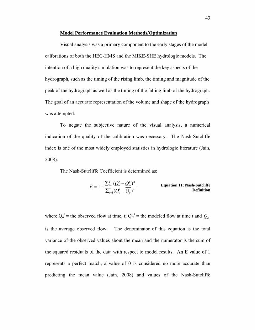
43
Model Performance Evaluation Methods/Optimization
Visual analysis was a primary component to the early stages of the model
calibrations of both the HEC-HMS and the MIKE-SHE hydrologic models. The
intention of a high quality simulation was to represent the key aspects of the
hydrograph, such as the timing of the rising limb, the timing and magnitude of the
peak of the hydrograph as well as the timing of the falling limb of the hydrograph.
The goal of an accurate representation of the volume and shape of the hydrograph
was attempted.
To negate the subjective nature of the visual analysis, a numerical
indication of the quality of the calibration was necessary. The Nash-Sutcliffe
index is one of the most widely employed statistics in hydrologic literature (Jain,
2008).
The Nash-Sutcliffe Coefficient is determined as:
21
21
)()(1
oto
Tt
tm
to
Tt
QQQQE
−∑−∑
−==
= Equation 11: Nash-Sutcliffe Definition
where Qot = the observed flow at time, t; Qm
t = the modeled flow at time t and oQ
is the average observed flow. The denominator of this equation is the total
variance of the observed values about the mean and the numerator is the sum of
the squared residuals of the data with respect to model results. An E value of 1
represents a perfect match, a value of 0 is considered no more accurate than
predicting the mean value (Jain, 2008) and values of the Nash-Sutcliffe

44
Coefficient less than zero (-∞<E<0) indicate that the mean is a better predictor
than the model.
3.3 Model Set Up: Case Studies
Hydrologic models using the HEC-HMS program were original
components of the Characterization and Assessment portion of the Regional
Stormwater Management Plans developed for two designated watersheds in New
Jersey. Both watersheds were identified as having water quality impairments that
were related to diffuse source pollution and flooding issues. The creation of a
Regional Stormwater Management Plan was to provide quantitative information
on how to address these storm related issues.
The location of the two case study watersheds within New Jersey can be
seen in Figure 2. The Troy Brook Watershed, located in Morris County, is
approximately 16 square miles. This watershed system discharges to the
Whippany River and eventually to the Passaic River. The Pompeston Creek
Watershed is located in Burlington County, NJ and is approximately 8.1 square
miles. The Pompeston Creek discharges directly into the Delaware River.

45
Figure 2: New Jersey Case Study Watersheds
As is the case for a great portion of New Jersey, these two watersheds
contain a large percentage of developed area considered urban land use. While
water quality may be a source of the impairment of the Troy Brook Watershed,
water quantity and flooding issues also affect the watershed in many ways.
3.3.1 GIS Input Data
The input data for all of the models that were prepared began with readily
available GIS data layers. These layers included the topography, land use, stream
layers and soil layers. All layers were acquired through the NJDEP GIS
download webpage (http://www.state.nj.us/dep/gis/).
The topography is represented by a 7.5 minute Digital Elevation Model
(DEM) generated by USGS to describe the terrain elevation. The resolution of
these standard DEMs 10-meters. The watershed boundary was delineated and
further subdivided into smaller, more manageable subbasins by using this
topography dataset and the HEC-GeoHMS software. The subbasins were only
necessary in the HEC-HMS model, as the MIKE SHE model uses the raster DEM
converted to its MIKE-SHE grid format (dfs2) for physical calculations.

46
The landuse of the watersheds was represented by the 2002 Land Use
Land Cover dataset using the Type 02 attribute, based on the photography
captured in the spring of 2002. The visual interpretation of these photographs is
prepared into a digital file, with distinguishable polygons representing a distinct
land use/land cover type (http://www.state.nj.us/dep/gis/lulc02shp.html). The
stream network was created in conjunction with the land use/land cover 2002
dataset.
The SSURGO digital dataset represents the soil distribution of the
watersheds. This dataset was developed by the Natural Resources Conservation
Service (NRCS), of the US Department of Agriculture, as a part of the National
Cooperative Soil Survey (http://www.state.nj.us/dep/gis/soilsshp.html).
These GIS data layers provide the necessary spatial data for these models.
The preparatory step for the HEC-HMS models is the use of the Geo-HMS
software that computes the metrics of input for the HEC-HMS model from the
topography dataset. Using this program, the watershed and its subbasins can be
delineated. All subbasin outlets are designated as hydrologic junctions where the
flow is calculated. Input parameters such as flow lengths and subbasin centroids
are calculated and prepared for input into the HEC-HMS model.
The MIKE-SHE model uses a .dfs2 grid file format for the physical
calculations of rainfall-runoff. This .dfs2 file format is generated from the
raster/grid GIS datasets. Functions within the ArcMAP GIS software allow for
the transformation of a polygon shapefile into a grid format. The grid is
converted to a .dfs2 format in the MIKE SHE modeling program.

47
3.3.2 The Pompeston Creek Watershed
Study Area
The Pompeston Creek Watershed, located in Burlington County, New
Jersey is approximately 8.1 square miles (Appendix A, Map 1). The watershed
system discharges to the Delaware River and contains part of the municipalities of
Moorestown, Delran, Riverton, and Cinnaminson. The Pompeston Creek
Watershed is comprised of 10 to 13 miles of river and more than 13 acres of
lakes. The stream is tidal to about 0.75 miles upstream of its discharge point to
the Delaware River which includes a freshwater tidal marsh.
The watershed was subdivided into thirteen subbasins that would represent
hydrologic units for calculations in the lumped parameter model, HEC-HMS (See
Figure 3 and Map 1, Appendix A). These subbasins were not used in the fully
distributed, MIKE SHE model.
Note the location of the water surface elevation gage in Figure 3 at the
outlet of Subbasin 12. This is the location within the watershed where the
elevation of the stream was measured over time. This information was used in the
calibration procedure.

48
Figure 3: The Pompeston Creek Watershed Study Area
Land Use
The land use in the Pompeston Creek Watershed is composed of
residential, commercial and industrial development with some minor open space.
According to 2002 data collected by the NJDEP, the land use of the Pompeston
Creek Watershed is 80% urbaniz. Land use information is shown in Table 3.
Based on aerial photography taken in 2002, the NJDEP created a data set

49
describing land use across the state. This land use/land cover information is
available in GIS and can be useful in the analysis of a watershed.
The distribution of the land use types within the Pompeston Creek
Watershed can be seen in Map 2 of Appendix A.
Table 3: NJDEP 2002 Land Use Data for Pompeston Creek Watershed Land Use Type Acres Square Miles PercentageAGRICULTURE 173.19 0.27 3.3 BARREN LAND 86.89 0.14 1.7 FOREST 328.04 0.51 6.3 URBAN 4168.87 6.51 80.0 WATER 30.24 0.05 0.6 WETLANDS 420.89 0.66 8.1
Total: 5208.12 8.14 100.0
Soils
The Pompeston Creek Watershed may further be characterized by its soils
(See Figure 4 and Map 3 of Appendix A). Within the Pompeston Creek
Watershed, soils are predominantly in the Sassafras and Woodstown series. The
Sassafras soil series, found mostly in the lower half of the watershed, consists of
well-drained and very deep soils formed from sandy marine and old alluvial
sediments (USDA/NRCS, 2002). The Woodstown series is mostly found in the
upper portion of the Pompeston Creek Watershed and follows the stream corridor.
This series consist of very deep, moderately well-drained soils in upland marine
terraces and old stream terraces (USDA/NRCS 2002). The Woodstown series are
characterized by their moderate infiltration rates and shallow water table (18–42
inches per year). Potential for surface water runoff is considered slow to
moderate for this soil series (USDA/NRCS, 2002). Slopes can be variable, from 0
to 30 percent slopes. The Galestown series is found along the main stem of the

50
lower Pompeston Creek. Galestown soils are characterized as very deep,
somewhat excessively drained soils with deep water tables (greater than 72
inches) (USDA/NRCS, 2002). Finally, soils classified as “Made Land” are
located at the mouth of the creek, where it drains into the Delaware River. Made
lands are defined by the NJDEP as dredged coarse material with a slope ranging
from 0 to 5 percent.
Figure 4: Pompeston Creek Soil Series
The SSURGO soil database that was used for this study provides the
characteristics of these soil components. Each soil type is designated a
“Hydrologic Group” based on the soil’s runoff potential. There are four

51
hydrologic soil groups, from A to D, where A generally has the greatest
infiltration capacity and D has the lowest infiltration, or highest runoff capacity.
Group A soils consist of sand, loamy sand or sandy loam that has low
runoff potential and high infiltration capabilities, even when thoroughly wetted.
These soils have a high rate of water transmission.
Group B soils consist of silt loam or loamy soils and have low infiltration
rates when thoroughly wetted. The infiltration rate is moderate when thoroughly
wetted, and the soils drain well for moderately fine to moderately course textures.
Group C soils are sandy clay loam. The infiltration rates are generally low
when wetted. These soils may have a moderately fine to a fine layer that slows
the transmission of water.
The Group D soils have the highest runoff potential. These soils are clay
loam, silty clay loam, sandy clay, silty clay or clay. These soils posses a low
infiltration rate and a high swelling potential when wetted, and could have a
permanent high water table or a clay layer at or near the surface making it nearly
impervious.
The section of the soil hydrologic group designated “Z” are those areas
that have not been classified. These areas represented relatively small areas
within the watersheds, therefore the characteristics of those soils closest to the
“Z” soils were used.
The soil components of the Pompeston Creek Watershed and the
corresponding soil hydrologic group can be found viewed in Figure 5.

52
Combinations of the hydrologic soil groups denote an area that is considered of
mixed attributes.
Figure 5: Pompeston Creek Soil Hydrologic Groups
Additional descriptive attributes can be found in the SSURGO database
that aid in the characterization of the physical characteristics. The estimated
drainage ability (poor to well), the percent of compaction, soil names and types
are some of these attributes.
Impervious Surfaces
The land use shapefile includes the information on the percent of the
impervious cover identified in the aerial photography. Each land use polygon is
designated a percent impervious and the overall impervious nature of the
watershed can be determined. An overview of the impervious coverage within
the Pompeston Creek Watershed can be found in Table 4. A map showing the

53
distribution of the percentage of impervious area throughout the watershed can be
found in Appendix A, Map 4.
Table 4: Pompeston Creek Watershed Impervious Surface
IS=Impervious Surface
acressquare
miles
IS
acresIS square
miles Percent
ISOverall Watershed, 13
subcatchments 5208.1 8.1 1304.7 2.0 25.0
Subbasin 8 261.3 0.4 85.0 0.1 32.5Subbasin 9 345.9 0.5 142.2 0.2 41.1
Subbasin 13 253.6 0.4 52.2 0.1 20.6Subbasin 12 698.6 1.1 108.9 0.2 15.6
Total Upper Basins 1559.5 2.4 388.3 0.6 24.9
The impervious nature of the entire 8.1 square miles watershed is
represented in the upper four subbasins (Subbasins 8, 9, 13 and 12). Observations
from these subbasins were used to calibrate both models.
Observed Precipitation Events
The Pompeston Creek Watershed was evaluated for the water surface
elevation at the Subbasin 12 outlet site for approximately nine months beginning
in April of 2005. Precipitation depths over time and flow over time were
considered for model input if the distribution was somewhat parabolic and the
volume of precipitation was over 0.5 inches and under 1.25 inches. This range
was determined as the area of interest, given that visible runoff would be expected
to begin after 0.5 inches of precipitation. Ninety percent of the rainfall events in
the Mid-Atlantic region are storms of one inch or less (Claytor and Schueler,
1996) so this range would contain events that are representative of regular
occurrences.

54
Three storm events were determined to be appropriate for use in
calibration and validation in the Pompeston Creek Watershed. The storm time
distribution and total precipitation depth can be seen in Table 5.
Table 5: Pompeston Creek Watershed Storm Events
Storm Date Length of Storm Total Precipitation
Depth (hours) (inches) 10/11/2005 35.5 0.84 10/24/2005 17.5 1.06 11/16/2005 6.75 0.76
An additional data set was obtained from a surface observation station
maintained by Automated Surface Observation System (ASOS) and reported
through the Rutgers NJ Weather and Climate Data Network
(http://climate.rutgers.edu/njwxnet/index.php). The station is located in Mount
Holly, NJ, approximately ten miles from the Pompeston Creek Watershed. This
data set was intended only to evaluate the sensitivity of precipitation distribution.
Observed Flow
Calibration for the four upstream subbasins was performed with the
observed flow that was measured at the outlet of Subbasin 12 (Figure 3).
Given that there exists no USGS gage to measure long term flow in the
watershed, this site was set up specifically for this modeling effort. A temporary
pressure transducer was installed at the bottom of the stream at this location to
record water depth. The depth and the corresponding flow were determined over
the course of several seasons to incorporate a variety of situations. The resulting
rating curve can be seen in Figure 6.

55
Stage Site 1-Pompeston Park y = 0.1788Ln(x) + 0.3553R2 = 0.796
0
0.2
0.4
0.6
0.8
1
1.2
1.4
0 5 10 15 20
Flow (cfs)
Stag
e H
eigh
t (ft
)
Figure 6: Rating Curve for the Pompeston Creek Watershed
Pompeston Creek Watershed HEC-HMS Model Set Up
Loss Rate The GIS layers of the land use and the soils were joined into one GIS layer
in the ArcGIS program. The newly created polygons contained both the attributes
of the land use and the soil properties. A query process in the ArcView
application was used to sort the groups of specific combinations of soil types and
land use types. A curve number for that polygon could then be assigned through
the use of the tables provided in the TR-55 (U.S. Soil Conservation Service,
1986). Curve numbers used for these study watersheds can be found in Table 1.
These individual CNs within each subbasin are then multiplied by the area
that they cover, added together and then divided by the total area in that subbasin
(see Equation 4). It was this single CN that is used to describe the characteristics
of the infiltration and runoff of a subbasin in the HEC-HMS model set up.
The other loss rate input parameters for input to the HEC-HMS hydrologic
model are based on the original CN, as described in Equation 2 and Equation 3.

56
Table 6 shows the originally determined input parameters that empirically
described the loss rate for the Pompeston Creek HEC-HMS model.
Table 6: Pompeston HEC-HMS Original Loss Rate Input Parameters Subbasin Area wt S I(a)
ID CN 1 73 3.7 0.7 2 76 3.2 0.6 3 74 3.5 0.7 4 78 2.8 0.6 5 76 3.2 0.6 6 83 2.0 0.4 7 83 2.0 0.4 8 79 2.7 0.5 9 81 2.3 0.5
10 84 1.9 0.4 11 67 4.9 1.0 12 84 1.9 0.4 13 81 2.3 0.5
S=Potential Maximum Retention (in) I(a)= Initial Loss/Initial Abstraction (in) Transform
The volume of runoff is transformed by being temporally distributed to the
stream flow (as in the shape of the hydrograph). This has been determined by
using the Snyder Unit Hydrograph Method (See Section 3.3.5). The two input
parameters required are the Snyder Lag time and the Snyder Peaking Coefficient.
Values of the Snyder Lag time were determined using Equation 5 and the
parameters derived from the GIS layers.

57
Table 7: Pompeston Creek Original Transform Parameters
Subbasin Snyder
Lag(tp)(hrs) 1 0.3380 2 0.4418 3 0.4320 4 0.4126 5 0.2802 6 0.3429 7 0.3732 12 0.4437 13 0.3383 9 0.3774 8 0.2873 10 0.3725 11 0.2375
The values for the Snyder Peaking Coefficient were all initially set at an
average default empirical value of 0.6 (Bedient and Huber, 1992).
Routing Method
The HEC-HMS model used a Muskingum Cunge Standard Routing
Method to simulate the flow in the stream. The reach length (ft) and energy slope
(ft/ft) were determined from the GIS topography. The simplified cross section
was modeled as a prism, with a bottom width of 5 feet in the upper watershed and
10 feet in the lower watershed (below water elevation gauge used for calibration).
A side slope of 1 horizontal unit for every vertical unit was used. Mannings n
values ranged from 0.02 to 0.07.

58
Pompeston Creek Watershed MIKE-SHE Model Set Up
The MIKE-SHE model set up does not require the assignment of an
empirical number such as the curve number to determine the runoff and
infiltration capacity of the watershed. This model performs the physical
calculations as described in Section 3.4 using the physical data input derived from
the GIS layers within the model domain. The overland flow module also uses the
Manning number to represent the flow delay.
An initial grid size of 10 meters was used in accordance with the
distributed resolution of the topography. This fine resolution created long
simulations times. The resolution was then decreased to a grid size of 50 meters
which provided simulations in a relatively reasonable time. It was determined
that after the model was further developed the grid size could be reduced if
desired.
The net rainfall fraction, representing the fraction of rainfall that is
available for overland flow, was originally set to 1, or 100% of the rainfall was
available for overland flow. This would assume that leaf interception and
evapotranspiration was negligible over the time period of the event.
In the MIKE-SHE model, there are several options for modeling the
rainfall-runoff processes in a watershed. For the purpose of this study, the
essential elements of the model should use a fully distributed, spatial database and
physically based equations. The input parameter databases, primarily those from
GIS, were used to provide a base of consistency between the HEC-HMS model
and the MIKE-SHE models.

59
Method A
Method A was comprised of three components: the overland flow module
solved using the finite difference method; a “Rivers and Lakes” module, which
describes the flow of the water within the channel and the climate module, which
organized the precipitation distribution over time and accounts for the percent of
rain available for runoff.
Input to the overland flow module (OL) consisted of the topography
database, the distributed input of the Manning M values, the detention storage of
the watershed and the initial water depth within the watershed depicting the initial
depth of water on the ground surface, used as an initial condition.
The topographic relief (10 meter X 10 meter) was the same as used to
determine the flow path in the HEC-GeoHMS model.
The Manning M was determined with the use of the land use file and
empirical relations (for the reciprocal, Manning n) based on Chow, 1988. Values
of Manning M could range between 100 (smooth surface, low resistance to flow)
down to 10 (thickly vegetated, high resistance to flow). A spatial distribution of
the original assigned Manning M values for the Pompeston Creek Watershed can
be found in Figure 7.

60
Figure 7: Pompeston Creek Input Manning M values
The original assigned value for the detention storage used a default value
of two centimeters (0.787402 in). This would be the depth of ponded water
allowed to accumulate on the surface of the land before flow would begin. The
value for the initial water depth, the initial condition for the overland flow
calculations, was set to zero.
Routing Method: MIKE 11
The “Rivers and Lakes” module of the MIKE model is the MIKE11
application software. This software has the components to provide a more
detailed analysis of the hydraulic functions of the watershed than the HEC-HMS
provides. However, for the purposes of this study, the stream channel was
modeled to replicate the stream channel created in the HEC-HMS hydrologic
model.
The stream network was created in the MIKE11 application using the
ArcGIS shapefile for the Pompeston Creek. This general line network is then

61
generated into a file that has elements where the flow is calculated (Q points) and
elements where the water surface elevation (h points) is calculated. These points
are spread along the network with the modeler determining the number by the
amount of chainages (links of sections of streams) that are formed upon the
network creation. The stream is allowed to accept overland flow input at each
stream node (chainage) that is created within the model.
The cross sections used in the MIKE11 model attempted to reproduce the
channel created in the HEC-HMS project. Cross Sections were of prism shaped,
with a side slope of 1:1 and a bottom width of five to ten feet. The channel
dimensions in both the HEC-HMS project and the MIKE-11 project were similar,
assumed cross sections. This study did not examine for the model sensitivity to
cross section dimension.
Method B
The “Method B” that was used to model the Pompeston rainfall runoff
patterns included all of the same parameters as contained in Method A. In
addition to the parameters that were used for the overland and channel flow
modules, three databases were added for the purpose of gaining a better
understanding of the distributed the soil infiltration function. These three
databases included: a module to include water movement in the unsaturated zone;
a module to include the movement of water in the saturated zone and a spatially
distributed grid layer depicting the level of impervious surface.
In the MIKE-SHE model, the unsaturated zone was modeled using a 2-
layer water balance method (See Section 3.4.5). This method requires the four

62
physical characteristics of soil infiltration: the water content at saturation, the
water content at field capacity, water content at wilting point and the saturated
hydraulic conductivity. Table 8 provides the initial input parameters that were
selected for use in the Pompeston MIKE-SHE Method B hydrologic model.
Table 8: Original Soil Property Parameters for Unsaturated Zone Model (Method B) ID Hydgrp* MUSYM** Water Content Water Content Water Content Saturated Hydraulic at Saturation(1) at field capacity(2) at wilting point(3) Conductivity (ft/day) (df 0.3) (df 0.1) (df 0.05) (df 2.83465) 0 Water X WATER 0 0 0 0.000 1 Galestown A GabB 0.417 0.217 0.05 39.998 2 A UddcB 0.432 0.232 0.05 39.998 3 Klej B GakB 0.432 0.232 0.05 25.998 4 Sand/Gravel A PHG 0.5 0.3 0.05 3.999 5 D UdrB 0.486 0.286 0.05 0.060 6 Sassafras B SabB 0.401 0.201 0.05 25.998 7 A URSAAB 0.486 0.286 0.05 39.998 8 Sassafras C SapkB 0.486 0.286 0.05 2.599 9 Downer B DocC 0.401 0.201 0.05 25.998
10 D MamnAv 0.417 0.217 0.05 0.060 11 C URSACB 0.486 0.286 0.05 2.599 12 Urban Land B/D HofB 0.4 0.2 0.05 7.999 13 B/D FmhAt 0.486 0.286 0.05 7.999 14 Sassafras C SaekB 0.486 0.286 0.05 2.599 15 Sassafras B SapB 0.486 0.286 0.05 25.998 16 Woodstown C WofkB 0.486 0.286 0.05 2.599 17 Keyport C KeoC 0.434 0.234 0.05 2.599 18 Fallsington B/D WofA 0.486 0.286 0.05 0.259 19 Sassafras C SaekA 0.486 0.286 0.05 2.599 20 Woodstown C WofkA 0.486 0.286 0.05 2.599 21 Woodstown C WofkB 0.486 0.286 0.05 2.599 22 B/D FanA 0.486 0.286 0.05 7.999 23 Keyport C KeoB 0.434 0.234 0.05 2.599 24 Shrewsbury C/D DobA 0.486 0.286 0.05 0.259 25 Sassafras C SaekA 0.486 0.286 0.05 2.599 26 Sassafras B SaeA 0.486 0.286 0.05 25.998 27 C/D CoeAs 0.486 0.286 0.05 0.799 28 Keyport C KeoA 0.434 0.234 0.05 2.599
29 C WofkA 0.486 0.286 0.05 2.599 * See Appendix B; **Map Unit Symbol; (1), (2) and (3): Rawls et al., 1982/52/; Cosby et al., 1984/44/;Rijtema, 1969,/55/ (4) NRCS http://www.mo10.nrcs.usda.gov/references/guides/properties/sathydcond.html

63
The model provides a default parameter for each of these features in the
event that the soil is not user characterized. These default numbers are shown in
parentheses under the column heading in Table 8.
The saturated zone was included as a necessary module that created the
opportunity to incorporate the “paved runoff coefficient” spatial gridded database
that represented the extent of the impervious area. The saturated zone was
modeled to provide initial conditions that would allow the unsaturated zone to
infiltrate according to its hydraulic properties. The initial default quantification of
these properties can be found in Table 9.
Table 9: Default input parameters for Saturated Zone Module Geological Layers Lower Level Aquifer -30 ft
Horizontal Hydraulic Conductivity 28.3465 ft/day
Vertical Hydraulic Conductivity 28.3465 ft/day Specific Yield 0.02 L3/L2/L Specific Storage 3.05E-05 L-1
Computational Layers Initial Potential Head -3.28 ft
Impervious Area
The intent of the creation of Method B in the MIKE-SHE modeling format
was to be able to spatially represent the amount of impervious area that the
watershed contains. The 2002 Land Use/Land Cover GIS shapefile was used to
determine the percentage impervious (see Figure 8 and Map 4 in Appendix A).
This GIS shapefile was transformed into a GIS grid file, and then into a dfs2 file
that is compatible with the MIKE-SHE modeling system.

64
Figure 8: Pompeston Creek Impervious Area
The impervious cover dfs2 file is to initiate the amount of precipitation
that is available for runoff by calculating the percentage available to the soil layer.
The model will automatically route the excess precipitation from the impervious
area directly to the stream nodes; this routing is based on the assumption that the
time steps of the simulation are longer than the time it would take for the
precipitation that hits the impervious area to make it to the stream (DHI, 2008).
This assumption is not always the case, particularly in event based modeling.
The breakdown of the impervious surface distribution in the Pompeston
Creek Watershed is found in Table 4. As discussed previously, the gauge for the

65
observed data is located at the outlet of Subbasin 12 (see Map 1, Appendix A).
This outlet was intended to represent the runoff from the upper four subbasins, 8,
9, 13 and 12. Together these subbasins contain 24.9% impervious area, whereas
the entire Pompeston Creek Watershed consists of 25% impervious area.
3.3.3 The Troy Brook Watershed
Study Area The Troy Brook Watershed (Appendix A, Map5 and Figure 9) is located in
eastern Morris County, New Jersey. The watershed is 12 miles northeast of
Morristown and approximately 25 miles from New York City. The watershed
drains approximately 16 square miles with the majority of the watershed lying
within the municipality of Parsippany-Troy Hills with lesser areas in Mountain
Lakes and Hanover Townships. The major lakes in the watershed include
Mountain Lake, Wildwood Lake, Intervale Lake, Parsippany Lake, Bee Meadow
Pond, Forge Pond, the Upper Pond at the former BASF Corporation Property and
the Pond at Sheraton Hotel. Major tributaries for Troy Brook include West Brook,
Eastmans Brook, the tributary from Intervale Lake and the tributary from
Mountain Lake. West Brook is located in the western edge of the Troy Meadows
and extends from Bee Meadow Pond to its confluence with Troy Brook.
Eastmans Brook is located in the south central portion of the watershed and
extends from Lake Parsippany to its confluence with Troy Brook. The Mountain
Lake tributary is located in the northwest portion of the watershed and extends
from Mountain Lake to its confluence with Troy Brook. The tributary from

66
Intervale Lake is located in the northern regions of the watershed flowing from
Wildwood Lake to Intervale Lake and then through Manor Lake and into Troy
Brook just south of Route 46. In addition there are several smaller tributaries and
ponds in the watershed.
Figure 9: The Troy Brook Watershed Study Area
Land Use
The land use in the Troy Brook Watershed ranges from low density
residential in Mountain Lakes, medium to high density residential through
Parsippany-Troy Hills, to wetlands in the Troy Meadows section of Parsippany-
Troy Hills. Hanover Township consists primarily of medium density and low

67
density residential. Hanover Township also has a significant transitional area
representing areas under development, where site preparation is present, but the
future use has not been realized. Refer to Map 6 in Appendix A for the map of
the Troy Brook watershed’s existing land uses.
According to data collected by the NJDEP, the land use of the Troy Brook
Watershed is 53% urbanized (Table 10).
Table 10: Troy Brook Land Uses 2002 Land Use Area Percentage of Watershed Area Square Miles %
Agriculture 0.08 0.5
Barren Land 0.05 0.3
Forest 3.37 20.9
Urban 8.55 53.1
Water 0.68 4.2
Wetlands 3.37 21.0 Total 16.11 100.0
Soils
The Troy Brook watershed may further be characterized by its soils.
Within the Troy Meadows, soils are predominantly Carlisle muck. This soil
series consists of very poorly drained and very deep soils formed in depressions
of lake plains, outwash plains, moraines, and floodplains. The ponding duration
is known to be long, from October through June, and the typical slopes range
from 0 to 2 percent (NJDEP/USDA NRCS, 2004). The remaining soils of the
watershed are variable. The Parsippany series are mostly found up-gradient of the
Troy Meadows and follow the stream corridor. The Parsippany series consist of
deep, poorly drained soils in extinct lake basins and near streams. The Parsippany
series are characterized by their slow infiltration rates, shallow water table,

68
resistance to erodibility, and are usually subject to seasonal flooding. Potential
for surface water runoff is considered high for this soil series (NJDEP/USDA
NRCS, 2004). The Riverhead soil series can be found in the northwest and north
regions of the drainage basin. This series has been classified as having very deep,
well-drained soils, derived from granitic material. Slopes can be extremely
variable, from 0 to 50 percent slopes. Due to their well-drained nature, surface
runoff potential is considered low to medium (USDA/NRCS, 2004). Spanning
the north and middle section of the watershed are the Rockaway soil series.
These soils can be categorized as being moderately well-drained, formed as till on
uplands. Slope can range from 30 to 60 percent (USDA/NRCS, 2001). Finally,
urban soil complexes exist throughout the center and northern regions of the
watershed. Urban soils differ from soils that have formed over centuries and
millenniums and thus do not have a uniform structure or known properties.
Rather, urban soils range from being extremely variable in texture and structure to
being uniformly heavily compacted soil material (Baumgartl, 1998). The
dominant soil series within the Troy Brook Watershed are depicted in Figure 10.
(RCE WRP, 2007)

69
Figure 10: Dominant Soil Series in the Troy Brook Watershed
Soils can also be classified according to their potential to infiltrate water.
As discussed previously, the Natural Resource Conservation Service (NRCS)
categorizes soils that have high infiltration rates, “A” soils, to those that have very
slow infiltration rates, or “D” soils. The soils that possess intermediate qualities
are classified in a continuum. Map 7 in Appendix A shows the soils of the Troy
Brook Watershed as defined by their hydrologic soil group (hydgrp).
Impervious
The land use shapefile includes the information on the percent of the
impervious cover identified in the aerial photography. Each land use polygon is
designated a percent impervious and the overall impervious nature of the
watershed can be determined. An overview of the impervious coverage within
the Troy Brook Watershed can be found in Table 11. A map showing the

70
distribution of the percentage of impervious area throughout the watershed can be
found in Appendix A, Map 8 and in Figure 11.
Table 11: Troy Brook Impervious Area Coverage acres sq mi IS acres IS sq mi % IS Overall watershed 10192.66 1488.711 14.60572 Upstream Subbasins 1 133.3 0.21 23.9 0.04 17.9 2 475.0 0.74 44.6 0.07 9.4 3 39.6 0.06 10.1 0.02 25.6 4 209.5 0.33 87.3 0.14 41.6 5 436.5 0.68 80.5 0.13 18.4 6 133.6 0.21 50.1 0.08 37.5 7 8.4 0.01 4.0 0.01 47.9 8 26.6 0.04 3.4 0.01 12.8 9 35.9 0.06 15.4 0.02 42.9 10 644.9 1.01 75.3 0.12 11.7 23 374.7 0.59 56.0 0.09 56.0 26 218.5 0.34 57.6 0.09 57.6 29 183.9 0.29 23.3 0.04 23.3 30 621.2 0.97 56.5 0.09 56.5 Total Upper Basins: 3541.7 588.1 16.6

71
Figure 11: Troy Brook Percent Impervious Surface Per Area
The impervious nature of the entire sixteen square mile watershed is
represented in the upper fourteen subbasins (Table 11). It was these subbasins
that were able to be calibrated with available observed data. The overall
watershed consisted of 14.6% impervious area, where the upper basins gauged for
calibration purposes consisted of 16.6% impervious area.
Observed Precipitation Events: Troy Brook Watershed The Troy Brook Watershed was evaluated for the water surface elevation at the
Subbasin 9 outlet site for approximately eight months beginning in February of

72
2008. Precipitation depths over time and flow over time were considered for
model input if the distributions were somewhat parabolic and the volume of
precipitation was over 0.5 inches and under 1.25 inches. This range was
determined as the area of interest, given that visible runoff would be expected to
begin after 0.5 inches of precipitation and given that storms under 1.25 inches
constitutes 90% of all rain events in the mid-Atlantic states (Claytor and Schueler,
1996). Storms providing over 1.25 inches of precipitation are considered above
the water quality design storm that stormwater management facilities are designed
to maintain.
Five storm events were determined to be appropriate for use in calibration
and validation in the Troy Brook Watershed. The storm time distribution and
total precipitation depth can be seen in Table 12.
Table 12: Troy Brook Watershed Storm Events
Storm Date Length of
Storm
Total Precipitation
Depth (hours) (inches)
2/1/2008 13 1.16 3/4/2008 16.5 0.81
3/19/2008 17 0.94 4/28/2008 18 1.07 5/9/2008 18.5 1.15
Observed Flow
Calibration for the four upstream subbasins was performed with the
observed flow that was measured at the outlet of Subbasin 9, as can be seen
located in Figure 9.

73
Given that there exists no USGS gage to measure long term flow in the
watershed, this site was set up specifically for this modeling effort. A pressure
transducer was placed at the bottom of the stream at this location. The water
surface elevation and the corresponding flow were determined over the course of
several seasons to incorporate a variety of situations. The resulting rating curve
can be seen in Figure 12.
Troy Brook Rating Curve at Homer y = 0.1681Ln(x) + 0.775R2 = 0.77
0
0.5
1
1.5
2
0 5 10 15 20 25 30 35 40 45
Flow (cfs)
Sta
ge H
eigh
t (ft)
Figure 12: Troy Brook Rating Curve
HEC-HMS Set Up: Troy Brook Watershed
A HEC-HMS model was set up for the Troy Brook watershed. The
simulation of precipitation and runoff processes consists of determining the
amount and rate of surface runoff reaching the Troy Brook and its tributaries and
routing it through a channel network. The model setup was done in two main
modules: the basin model and meteorological model. The basin model contains
watershed elements, properties and connectivity. The meteorological model
contains precipitation intensity distribution over time.

74
Loss Rate
As with the Pompeston Creek HEC-HMS model, the curve number was
determined as a function of land use, hydrologic soil group and available soil
moisture. The 1995 land use land cover data coverage available from the NJDEP
GIS database, and the NRCS SSURGO soils were used to determine average soil
moisture condition curve numbers for each land use and soil combination in the
Troy Brook watershed. The composite (area weighted average) curve numbers
were obtained using spatial analysis techniques and spatial databases within GIS.
Areas with unique combinations of land use and soil type, and
consequently hydrologic soil groups, were obtained by overlaying land use and
soil datasets. These overlay processes created several polygons representing
distinct combinations of these characteristics. Each of these polygons was
assigned a curve number using tables published by the SCS in Technical Report
55 (USDA, 1986). The table of average soil moisture CNs used for these study
watersheds was presented in Table 1.
Transform
The transformation of the excess runoff to stream flow was performed
using the Synder Unit Hydrograph, in a similar manner to the Pompeston Creek
HEC-HMS model. The two input parameters required are the Snyder Lag time
and the Snyder Peaking Coefficient. Values of the Snyder Lag time were
determined using Equation 5 and the parameters derived from the GIS layers
(Table 13).

75
Table 13: Troy Brook Original Transform Parameters
Subbasin Snyder Lag
Time (tp hrs)
1 1.889 2 2.418 3 0.93 4 1.83 5 2.375 6 1.592 7 0.766 8 0.966 9 0.912
10 2.852 23 2.119 26 2.099 29 1.463 30 2.361
The values for the Snyder Peaking Coefficient were all initially set at an
average default empirical value of 0.6 (Bedient and Huber, 1992).
Routing Method
The HEC-HMS model used a Muskingum Cunge Standard Routing
Method to simulate the flow in the stream. The reach length (ft) and energy slope
(ft/ft) were metrics determined from the GIS topography. The simplified cross
section was modeled as a prism, with a bottom width of 5 feet in the upper
watershed and tributaries and 10 feet on the main stem. A side slope of 1
horizontal unit for every vertical unit was used. Mannings n values ranged from
0.026 to 0.034.
Troy Brook Watershed MIKE-SHE Set Up
The MIKE-SHE model for the Troy Brook Watershed was set up in a
similar manner as the Pompeston Creek Watershed MIKE-SHE model. There is
no assignment of curve numbers for the method used for the overland flow

76
module. All data required for slopes, centroid lengths and model domain were
acquired from the GIS data layers. This overland flow module does use the
Manning number, an empirical coefficient, to represent the flow delay in this
physical model.
An initial grid size of 10 meters was used in accordance with the
distributed resolution of the topography. This fine resolution created long
simulations times. The resolution was adjusted to a grid size of 26 meters which
provided simulations in a relatively reasonable time. It was determined that after
the model was further developed the grid size could be reduced if desired.
The Troy Brook Watershed rainfall-runoff was modeled in MIKE-SHE
using solely Method A, the overland flow module without soil infiltration
capabilities.
Method A: Troy Brook
Method A was compiled in a similar process as Method A for the
Pompeston Creek modeling study. The principal process during the simulation
using Method A is the overland flow, with input parameters including
topography, Manning M values, detention storage and initial water depth.
The spatial distribution of the Mannings M roughness coefficients can be
seen in Figure 13. Higher values of Mannings M depict the smoother surfaces
expected to produce runoff more readily than lower numbers. The Manning M
value has been reported to be the inverse of assigned Manning’s n values,
however this remains a calibratable parameter.

77
Figure 13: Troy Brook Manning M values
The original assigned value for the detention storage used a default value
of two centimeters (0.787 in). This would be the depth of ponded water allowed
to accumulate on the surface of the land before flow would begin.
The value for the initial water depth, the initial condition for the overland
flow calculations, was set to zero.
Routing Method: MIKE 11
The routing for the stream channel in the Troy Brook was performed in a
similar manner as was performed in the Pompeston Creek MIKE-SHE model.

78
3.4 Planning
The lumped parameter models for both the Pompeston Creek Regional
Stormwater Management Plan and the Troy Brook Regional Stormwater
Management Plan were the primary models used to bring the plan to completion.
In both watersheds, the model parameters were adjusted to theoretically capture
the change in runoff potential with the change in land use. Alterations in the
curve number were used as the primary factor used to educate stakeholders in the
relation of impervious cover and poorly draining soils to the effects of the
stormwater volume and velocity within the stream network. Per cent in the curve
number were used in the model and the resultant volumes were used to show
watershed sensitivity to the curve number.
“Design” precipitation events were employed to depict potential output
scenarios. These 24-hour design rain events are developed by statistical analysis
of rainfall records, although the temporal distribution may not be what is seen
occurring in actuality (Ubonis, 1979). Data used for the two case studies
presented in Table 14 were obtained from the Natural Resources Conservation
Service (NRCS) Technical Bulletin 2004-4.0 (Birckhead, 2005), based on data
obtained from the statistical estimates of rainfall amounts performed by the
National Oceanographic and Atmospheric Administration (NOAA).

79
Table 14: Design Storm Rainfall Depths TYPE III STORM Morris County
24-HR RAINFALL (INCHES)
Burlington County 24-HR
RAINFALL (INCHES)
2-Year Storm 3.3 3.4 10-Year Storm 5.2 5.2 100-Year Storm 7.5 8.8
The distributed models were not used in the original planning efforts. The
HEC-HMS was able to portray the role of infiltration as to the effects on the
stream. However, the internal processes that could manage the magnitude of the
runoff could not be modeled within the capacity of the lumped parameter model.
The spatially distributed function, including the cell to cell calculation of the
runoff processes was determined to be necessary in order to represent the
management options that should be considered for a strormwater management
plan. The functioning of the MIKE SHE model was evaluated on the observed
data used in the calibration and validation efforts.

80
4. Results
Model results revealed various complexities involved in the hydrologic
modeling of the urban watershed. The two urban watersheds demonstrated the
importance of properly quantifying the urban nature of impervious surfaces and
soils, and the two types of hydrologic models demonstrated the importance of
accurate input data.
4.1 Pompeston Creek Watershed Case Study
The Regional Stormwater Management Plan for the Pompeston Creek
Watershed included simulations with HEC-HMS, a lumped parameter hydrologic
model. The waterways in this watershed were impaired by high bacteria and
phosphorus levels and exhibited a poor overall evaluation regarding the
macroinvertebrate community (RCE WRP, 2007). Although the urban land use is
primarily low and medium density residential development, the overall
impervious nature of the watershed is 25%. Delineating this watershed into
several subbasins, the model was able to simulate the processes of runoff and the
hydrologic impacts of higher volume and velocity contributions to the streams
that would potentially contribute to lower water quality conditions. Much of the
modeling effort revolved around properly characterizing the curve number and
determining methods that would reduce the curve number and infiltrate more
precipitation on site.
It became clear that these lumped models were only able to explain the
processes in general and with an emphasis on an empirical parameter that is

81
primarily used for calibration. Thus, the MIKE-SHE model was used to
determine if a fully distributed, physical model could be used in an effort to
identify problems and solutions with a more site specific method using the same
available input data.
4.1.1 Lumped/Empirical Calibration
The Pompeston Creek Watershed HEC-HMS model was primarily
calibrated by visual analysis and optimization of parameters, ultimately using an
objective function for intercomparison of simulations that were visually deemed
appropriate. The Nash-Sutcliffe Coefficient was the objective function used to
optimize the model representation for the purposes of this.
Calibration to achieve a set of best fit parameters for the Pompeston Creek
HEC-HMS lumped parameter model was performed on the storm event that
occurred on November 16, 2005. The total precipitation for this event was 0.728
inches over a 3.5 hour period and the five day antecedent moisture condition was
recorded to be 0.3 inches of precipitation. The resultant calibration provided a
Nash-Sutcliffe efficiency coefficient of E=0.611, indicating that the model
predictions are more accurate than the mean of the observed data (E=0), but
skewed closer to being a perfect match (E=1). The resultant hydrograph, along
with the hyetograph, can be viewed in Figure 14.
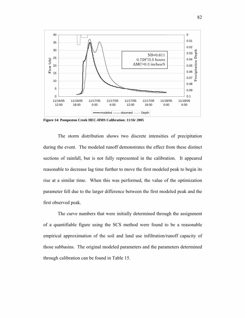
82
Figure 14: Pompeston Creek HEC-HMS Calibration: 11/16/ 2005
The storm distribution shows two discrete intensities of precipitation
during the event. The modeled runoff demonstrates the effect from these distinct
sections of rainfall, but is not fully represented in the calibration. It appeared
reasonable to decrease lag time further to move the first modeled peak to begin its
rise at a similar time. When this was performed, the value of the optimization
parameter fell due to the larger difference between the first modeled peak and the
first observed peak.
The curve numbers that were initially determined through the assignment
of a quantifiable figure using the SCS method were found to be a reasonable
empirical approximation of the soil and land use infiltration/runoff capacity of
those subbasins. The original modeled parameters and the parameters determined
through calibration can be found in Table 15.
0
5
10
15
20
25
30
35
40
11/16/0512:00
11/16/0518:00
11/17/050:00
11/17/056:00
11/17/0512:00
11/17/0518:00
11/18/050:00
11/18/056:00
Flo
w (
cfs)
0
0.01
0.02
0.03
0.04
0.05
0.06
0.07
0.08
0.09
0.1
Pre
cipi
tati
on D
epth
modeled observed Depth
NS=0.6110.728”/3.5 hours
AMC=0.3 inches/5

83
Table 15: Parameters for Pompeston HEC-HMS Initial Calibrated Initial Calibrated Initial Calibrated Initial Calibrated
Basin CN CN Ia Ia Lag Time Lag Time Peaking Peaking
8 79.4 77 0.52 0.1 1.69 0.363 0.6 0.27
9 81.1 78 0.47 0.1 2.22 0.726 0.6 0.36
13 81.1 81 0.47 0.1 1.99 0.847 0.6 0.36
12 84.7 86 0.36 0.1 2.61 2.541 0.6 0.18
The percent change in the estimated and the calibrated curve number
ranged from 0.1 percent to 3.8 percent throughout the four subbasins (Table 16),
with small changes resulting in increases in runoff volume. These distinct
changes should be viewed as a range of potential change, since these four
subbasins are ultimately “lumped” together for the purposes of the calibration.
The change in the curve numbers show the smallest percent change that was
necessary to create a calibrated model that better represents this watershed.
The initial abstraction (Ia) percent change from the original parameters to
the calibrated parameters showed a range of 72 to 81 percent difference (Table
16). Although the Ia is empirically related to the potential maximum surface
retention (S) in the watershed, which is empirically related to the curve number,
for the purpose of the calibration, these parameters moved independently. The
reduction of the depth of the Ia created the situation where the maximum
percentage of precipitation would be represented early in the hydrograph, to
correspond to the minimal retention capacity within the watershed.
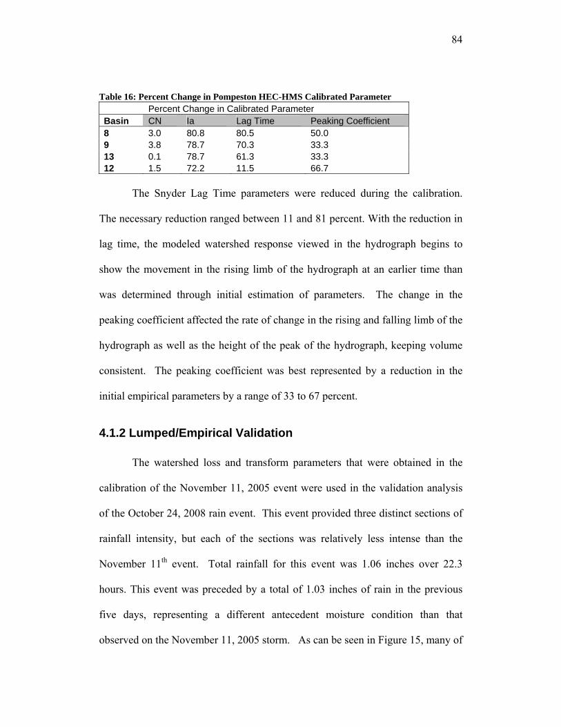
84
Table 16: Percent Change in Pompeston HEC-HMS Calibrated Parameter Percent Change in Calibrated Parameter Basin CN Ia Lag Time Peaking Coefficient 8 3.0 80.8 80.5 50.0 9 3.8 78.7 70.3 33.3 13 0.1 78.7 61.3 33.3 12 1.5 72.2 11.5 66.7
The Snyder Lag Time parameters were reduced during the calibration.
The necessary reduction ranged between 11 and 81 percent. With the reduction in
lag time, the modeled watershed response viewed in the hydrograph begins to
show the movement in the rising limb of the hydrograph at an earlier time than
was determined through initial estimation of parameters. The change in the
peaking coefficient affected the rate of change in the rising and falling limb of the
hydrograph as well as the height of the peak of the hydrograph, keeping volume
consistent. The peaking coefficient was best represented by a reduction in the
initial empirical parameters by a range of 33 to 67 percent.
4.1.2 Lumped/Empirical Validation
The watershed loss and transform parameters that were obtained in the
calibration of the November 11, 2005 event were used in the validation analysis
of the October 24, 2008 rain event. This event provided three distinct sections of
rainfall intensity, but each of the sections was relatively less intense than the
November 11th event. Total rainfall for this event was 1.06 inches over 22.3
hours. This event was preceded by a total of 1.03 inches of rain in the previous
five days, representing a different antecedent moisture condition than that
observed on the November 11, 2005 storm. As can be seen in Figure 15, many of

85
the important aspects of the hydrograph are not well represented. All three of the
observed peaks begin to rise before the modeled peaks, indicating an even lower
lag time and/or lower initial abstraction. The volume is also over predicted using
these model parameters, particularly in the third peak. The storm distribution,
greater antecedent moisture and lower intensity could contribute to the lower
Nash-Sutcliffe efficiency parameter of -3.49.
Figure 15: Pompeston Creek HEC-HMS Validation: 10/24/ 2005
4.1.3 Mount Holly Precipitation Data Set
In evaluating the potential contributions to the inaccuracies in the original
lumped parameter calibration effort, an alternate input data set representing the
precipitation measurements recorded at a nearby climate station was simulated
against the observed data in the Pompeston Creek Watershed for the storm event
on 11/16/05. This data set achieved a Nash-Sutcliffe efficiency coefficient of
0
5
10
15
20
25
30
35
10/24/0512:00
10/25/050:00
10/25/0512:00
10/26/050:00
10/26/0512:00
10/27/050:00
10/27/0512:00
Flo
w (
cfs)
0
0.02
0.04
0.06
0.08
0.1
Pre
cipi
tati
onModeled Observed Precipitation
NS=-3.491.057”/22.3 hrs AMC=1.03 inches/5 days

86
0.966, matching well the rising limb, the peak height of two separate peaks and
the timing of the falling limb (Figure 16).
Figure 16: Pompeston Creek HEC-HMS alternate precipitation data for calibration
The best fit parameter set was then used for a validation simulation with
the precipitation data collected that was also collected at this alternate site.
Results were less than optimal, producing a Nash-Sutcliffe efficiency coefficient
of -91. 7 (Figure 17). The effect of the varying antecedent moisture condition is
evident in the timing of the rising limb, but this alternate data does not appear to
represent the effect of the precipitation distribution observed in the stream as was
seen in the earlier data set.
0
5
10
15
20
25
30
35
40
11/16/0514:24
11/16/0519:12
11/17/050:00
11/17/054:48
11/17/059:36
11/17/0514:24
11/17/0519:12
11/18/050:00
11/18/054:48
Flo
w (
cfs)
0
0.2
0.4
0.6
0.8
1
1.2
1.4
Pre
cipi
tati
on
Modeled Observed Precipitation
NS=0.9660.87”/4.5 hours AMC=0.3 inches/5 days

87
Figure 17: Pompeston Creek Alternate Precipitation Data for Validation
4.1.4 Lumped/Empirical Sensitivity
An analysis of the parameter sensitivity was performed using the October
25th storm event. The model parameters were adjusted for points greater and
lesser than the optimal parameter determined in the calibration, and the effect on
the optimization parameter, the Nash-Sutcliffe Efficiency Coefficient, was
calculated.
Adjustment of the parameters was performed in stages on a percentage
basis to allow the larger empirical parameters to fluctuate a proportional amount
compared to the parameters with a smaller magnitude.
The sensitivity analysis demonstrated that small deviations in the three
parameters of initial abstraction, Snyder lag time and the Snyder Peaking
Coefficient produced a generally bilateral curvelinear deviation from the optimal
(Figure 19, 20 and 21). The Curve Number is more reactive to percent deviations
in its quantification and particularly sensitive to overestimation of this empirical
parameter (Figure 18).
0
20
40
60
80
100
120
10/24/05 12:00 10/25/05 0:00 10/25/05 12:00 10/26/05 0:00 10/26/05 12:00 10/27/05 0:00
Flow
(cfs
)
0
0.1
0.2
0.3
0.4
0.5
0.6
0.7
0.8
Prec
ipita
tion
(in)
Modeled Observed Precipitation
NS=-91.7 2.06”/ 22 hrs
AMC=1.03 inches/5

88
Curve Number Sensitivity
-3
-2.5
-2
-1.5
-1
-0.5
0
0.5
1
-25 -20 -15 -10 -5 0 5 10 15 20 25
Per Cent Deviation
Cor
resp
ondi
ng N
S C
oeff
icie
nt
Figure 18: Curve Number Sensitivity
Abstraction Sensitivity
0
0.2
0.4
0.6
0.8
-100 -50 0 50 100 150 200 250
Per Cent Deviation
Cor
resp
ondi
ng N
S C
oeff
icie
nt
Figure 19: Intial Abstraction Sensitivity
Snyder Lag Time Sensitivity
00.10.20.30.40.50.60.7
-30 -20 -10 0 10 20 30 40 50 60
Per Cent Deviation
Cor
resp
ondi
ng N
S C
oeff
icie
nt
Figure 20: Snyder Lag Time Sensitivity

89
Peaking Coefficient Sensitivity
0.54
0.56
0.58
0.60.62
0.64
0.66
-25 -20 -15 -10 -5 0 5 10 15 20 25
Per Cent Deviation
NS
Coe
ffic
ient
Figure 21: Peaking Coefficient Sensitivity 4.1.4 Distributed/Physical Calibration: Method A
Two variations of MIKE SHE models were developed for the Pompeston
Creek Watershed, Methods A and B. The more simplistic physical model that
focuses on overland flow as the primary effect on the hydrograph contains only a
small number of parameters that could be calibrated. Calibration efforts for the
November 16, 2005 storm event were attempted after model assemblage with data
layers similar to the HEC-HMS lumped parameter model. Default values for the
detention storage and the initial water depth in the watershed were reduced to
their lowest levels, given the urban nature of the watershed.
Extensive alterations of the Manning’s M value were necessary to provide
a modeled hydrograph that showed some of the characteristics of the observed
response. Original Manning’s M values were assigned to land uses as the
reciprocal of the assigned Manning’s n values. Although Manning’s n values are
typically used to represent the roughness coefficient of a stream corridor, with
distributed models, the entire watershed is treated like a large drainage channel.
However, the Manning’s M value used in the MIKE-SHE model is not well

90
represented in the literature. Use of the reciprocal of the Manning’s n did not
provide a value within an acceptable range. These reciprocals required reduction
by 73 to 99.5% of their original assignment to be able to provide a reasonable
stream flow response to overland flow (Table 17).
Table 17: Best Fit Manning's M Values
2002 Land Use Category Manning’s
n Manning’s
M Mannings
M Assigned Assigned Calibrated AGRICULTURAL WETLANDS (MODIFIED) 0.05 20.00 4.5 ALTERED LANDS 0.035 28.57 7.5 ARTIFICIAL LAKES 0.04 25.00 6 ATHLETIC FIELDS (SCHOOLS) 0.03 33.33 9 COMMERCIAL/SERVICES 0.03 33.33 9 CONIFEROUS BRUSH/SHRUBLAND 0.07 14.29 3 CONIFEROUS FOREST (10-50% CROWN CLOSURE) 0.1 10.00 0.5 CONIFEROUS WOODED WETLANDS 0.09 11.11 1.5 CROPLAND AND PASTURELAND 0.04 25.00 6 DECIDUOUS BRUSH/SHRUBLAND 0.1 10.00 0.5 DECIDUOUS FOREST (>50% CROWN CLOSURE) 0.1 10.00 0.5 DECIDUOUS SCRUB/SHRUB WETLANDS 0.1 10.00 0.5 DECIDUOUS WOODED WETLANDS 0.1 10.00 0.5 DISTURBED WETLANDS (MODIFIED) 0.06 16.67 4 EXTRACTIVE MINING 0.05 20.00 4.5 FORMER AGRICULTURAL WETLAND (BECOMING SHRUBBY) 0.06 16.67 4 FRESHWATER TIDAL MARSHES 0.06 16.67 4 HERBACEOUS WETLANDS 0.07 14.29 3 INDUSTRIAL 0.02 50.00 12 INDUSTRIAL/COMMERCIAL COMPLEXES 0.02 50.00 12 MANAGED WETLAND IN MAINTAINED LAWN GREENSPACE 0.07 14.29 3 MIXED DECIDUOUS/CONIFEROUS BRUSH/SHRUBLAND 0.1 10.00 0.5 MIXED FOREST (>50% CONIFEROUS WITH >50% CROWN CLOSURE) 0.1 10.00 0.5 MIXED URBAN OR BUILT-UP LAND 0.04 25.00 6 NATURAL LAKES 0.04 25.00 6 OLD FIELD (< 25% BRUSH COVERED) 0.03 33.33 9 ORCHARDS/VINEYARDS/NURSERIES/HORTICULTURAL AREAS 0.05 20.00 4.5 OTHER AGRICULTURE 0.035 28.57 7.5 OTHER URBAN OR BUILT-UP LAND 0.03 33.33 9 RECREATIONAL LAND 0.03 33.33 9 RESIDENTIAL, HIGH DENSITY, MULTIPLE DWELLING 0.02 50.00 12
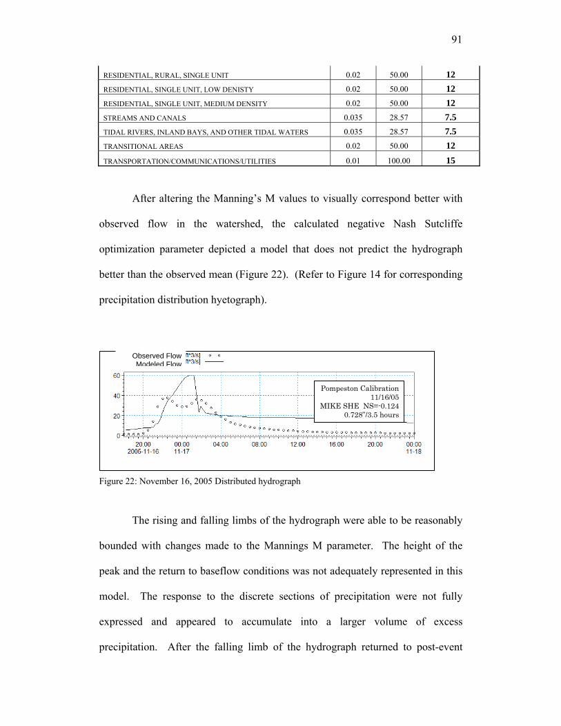
91
RESIDENTIAL, RURAL, SINGLE UNIT 0.02 50.00 12 RESIDENTIAL, SINGLE UNIT, LOW DENISTY 0.02 50.00 12 RESIDENTIAL, SINGLE UNIT, MEDIUM DENSITY 0.02 50.00 12 STREAMS AND CANALS 0.035 28.57 7.5 TIDAL RIVERS, INLAND BAYS, AND OTHER TIDAL WATERS 0.035 28.57 7.5 TRANSITIONAL AREAS 0.02 50.00 12
TRANSPORTATION/COMMUNICATIONS/UTILITIES 0.01 100.00 15
After altering the Manning’s M values to visually correspond better with
observed flow in the watershed, the calculated negative Nash Sutcliffe
optimization parameter depicted a model that does not predict the hydrograph
better than the observed mean (Figure 22). (Refer to Figure 14 for corresponding
precipitation distribution hyetograph).
Figure 22: November 16, 2005 Distributed hydrograph
The rising and falling limbs of the hydrograph were able to be reasonably
bounded with changes made to the Mannings M parameter. The height of the
peak and the return to baseflow conditions was not adequately represented in this
model. The response to the discrete sections of precipitation were not fully
expressed and appeared to accumulate into a larger volume of excess
precipitation. After the falling limb of the hydrograph returned to post-event
Pompeston Calibration 11/16/05
MIKE SHE NS=-0.124 0.728”/3.5 hours
Observed Flow Modeled Flow

92
baseflow conditions, the modeled hydrograph overpredicted flow and showed
minimal reaction to the end of the precipitation event.
4.1.5 Distributed/Physical Validation: Method A
The model parameters used in the November 11, 2005 calibration run of the
Pompeston Creek Watershed were used to simulate the October 24, 2005 storm
event for validation effort purposes. The resultant hydrograph (Figure 23) does
appear to be reacting to the various intensities of precipitation, although the
timing and magnitude of runoff are of low simulation quality, as a Nash-Sutcliffe
efficiency coefficient of -11.05 reflects.
Figure 23: October 24, 2005 Pompeston Creek Watershed Distributed Method A validation Run
As in the November 11, 2005 calibration run, the modeled values are over
predicted for the tail end of the hydrograph, but the multiple peaks that comprise
the streams reaction to the storm are also over predicted.
4.1.6 Distributed/Physical Sensitivity: Method A
The parameters that are able to be used to calibrate a physical model are
obviously more limited than those of an empirical model. The effects of
magnitude changes in the Mannings M values that are used to correspond to land
use have been modified to evaluate the effect on the resultant hydrograph.
Pompeston Validation NS=-11.05 10/24/05 MIKE SHE 1.057”/22.3 hrs AMC=1.03 inches/5 days
Observed Modeled

93
Figures 24 through 27 depict the output hydrograph results of alterations
to the Mannings M. During this exercise, it was determined that a 10 percent
increase in the parameter would have provided a more accurate hydrograph, with
a Nash Sutcliffe Efficiency Parameter, E= -0.05.
Figure 24: 10% decrease in Manning M
The reduction in Manning M by 10% appears to have only a slight affect
on the hydrograph, as evidenced by the peak remaining at the same time and the
same intensity. A small change in the rising limb of the hydrograph appears to
have the effect of lowering the volume under the curve.
Figure 25: 20% decrease in Manning M
Observed Modeled
NS=-0.167
NS=-0.435
Observed Modeled

94
A 20 percent reduction in the Manning’s M value decreases the peak flow,
the volume of the water under the hydrograph and shortens the resultant affect
that the precipitation has on the stream (See Figure 25). This appears to have
little effect on the return to baseflow seen in the observed data.
Figure 26: 10% increase in Manning M
In the scenario where the Mannings M was increased by 10 percent
(Figure 26), an increase in the modeled accuracy resulted. The modeled
hydrograph still failed to show the effects of the discrete sections of rainfall, as
the observed and the lumped parameter model was able to show. The tail end of
the modeled hydrograph showed the same slow course toward baseflow as seen in
the previous distributed model scenarios.
Figure 27: 20% increase in Manning M
Observed Flow Modeled Flow
NS=-0.051
Observed Flow Modeled Flow
NS=-0.267

95
By increasing the Mannings M value by 20 percent over the watershed
(Figure 27), the peak flow of the hydrograph was higher and the volume of flow
under the hydrograph increased. A smoothness of the first large peak continues to
dominate in the distributed model, with the second peak being only a small
artifact. It is unclear whether the second peak is a reaction to the discrete sections
of precipitation or if there are other contributing factors.
The overall outcome of the Manning M sensitivity analysis (Figure 28)
suggests that optimal parameters could exist within a range of values, but would
likely benefit from an increase in accuracy in the spatial distribution of assigning
parameters.
Manning M Sensitivity
-0.5
-0.45
-0.4
-0.35
-0.3
-0.25
-0.2
-0.15
-0.1
-0.05
0-25 -20 -15 -10 -5 0 5 10 15 20 25
Percent Change
Nas
h-Su
tclif
fe E
ffici
ency
Coe
ffici
ent
Figure 28: Manning M Sensitivity in Method A
4.1.7 Distributed/Physical Alternative Method: Method B
The MIKE SHE model offers several options for representing the
hydrological response of an urban watershed. In an alternative method attempting
to better characterize the urban runoff due to impervious surfaces and the effect of

96
the infiltration capacity of the soils, additional components were added to the
modeling scenario. These additional components included a 2-layer water
balance of the unsaturated zone, a general/default description of the saturated
zone, a drainage component and an impervious surface layer that details the
percent impervious according to the land use GIS layer.
Initial input parameters necessary to represent the infiltration properties of
the soils in the watershed are shown in Table 8. During calibration efforts, it was
determined that these assigned parameters overestimated the infiltration capacity
and therefore the hydraulic conductivity was reduced. Preliminary reductions
decreased the hydraulic conductivity by one order of magnitude. Further
calibration efforts adjusted these parameters with the extent and location of the
soils as a contributing qualifying factor. The spatial distribution of the hydraulic
conductivity assigned to the Pompeston Creek Watershed can be viewed in Figure
29.

97
Figure 29: Pompeston Creek Distributed Hydraulic Conductivity
The November 16, 2005 and the October 24, 2005 precipitation event
were simulated in order to provide information on how the model is predicts basin
outflow according to the event data. The results are shown in Figure 30 and Figure
31 below.
Figure 30: November 16, 2005 Pompeston Hydrograph: Method B Distributed Model
Pomp1116_discharge [ft̂ 3/s]Discharge [ft̂ 3/s]
21:002005-11-16
00:0011-17
03:00 06:00 09:00 12:00 15:00 18:00 21:00 00:0011-18
0
10
20
30
Observed Flow Modeled Flow Pompeston Calibration
MIKE-SHE 11/16/05 Method B NS=0.011
0.728”/3.5 hours

98
The October 24, 2005 storm event was also simulated using these added
components of impervious surfaces and soil infiltration parameters. The results
can be found in Figure 31 below.
Figure 31: October 24, 2005 Pompeston Method B Distributed Model
4.1.8 Distributed/Physical Sensitivity: Method B
The overall hydraulic conductivity parameters were altered to determine
the level of sensitivity that existed in the parameters used for calibration. The
resulting Nash-Sutcliffe Coefficient and the resulting correlation coefficient can
be seen in Figure 32.
-8
-7
-6
-5
-4
-3
-2
-1
0
1
-40 -20 0 20 40 60 80 100 120
Percent Deviation in HC value
Corr
espo
ndin
g Na
sh-S
utcl
iffe
Coef
ficie
nt
Figure 32: Sensitivity of the Pompeston MIKE-SHE model to alterations in the hydraulic conductivity parameter
Pomp1024val [ft^3/s]Discharge [ft^3/s]
ME 13 8737
00:002005-10-25
12:00 00:0010-26
0
5
10
15
20
25
Observed Flow Modeled Flow
Pompeston Validation MIKE-SHE Method B NS=-7.71 1.057”/22.3 hrs AMC=1.03 inches/5 days

99
However, visual analysis of these simulations shows a more comparable
reaction to the precipitation temporal intensity when the hydraulic conductivity is
decreased thirty percent (Figure 33). However, this reduction results in lower
coefficients for the Nash-Sutcliffe.
Figure 33: Hydraulic conductivity sensitivity hydrographs using Pompeston Creek calibration simulation of 11/16/05.
P o m p 1 1 1 6 _ d is ch a rg e [ft^3 /s ]D isch a rg e [ft^3 /s ]
2 0 :002 0 05 -11 -1 6
00 :0011 -17
0 4 :00 08 :00 0
1 0
2 0
3 0
Pomp1116_discharge [ft 3̂/s]Discharge [ft 3̂/s]
21:002005-11-16
00:0011-17
03:00 06:00 0
10
20
30
P o m p 1 1 1 6 _ d i s c h a r g e [ f t ^ 3 / s ]D i s c h a r g e [ f t ^ 3 / s ]
2 0 : 0 02 0 0 5 - 1 1 - 1 6
0 0 : 0 01 1 - 1 7
0 4 : 0 0 0 8 : 0 0 0
1 0
2 0
3 0
4 0
-30%
0
+60%

100
4.1.9 Distributed Method: Method B1
To determine the effect of the impervious cover layer on the fully
distributed model with the soil infiltration capacity being represented by the 2-
layer water balance, the impervious layer was removed from calculations after the
validation effort was complete. This was performed on the October 25, 2005
storm event (Figure 34).
Figure 34: Pompeston Creek October 25, 2005 Method B1
When compared with the original Method B (Figure 30) which included
the unsaturated zone infiltration parameters and the impervious surface coverage,
the effect of the impervious area can be seen. Without the impervious area
coverage inserted into the simulation, an early spike in the peak flow does not
exist and the flow rises slower, and higher than that previously modeled or than
that observed.
Pomp1024val [ft^3/s]Discharge [ft^3/s]
ME 14 5385
00:002005-10-25
12:00 00:0010-26
0
5
10
15
20
25
Observed Flow Modeled Flow
Pompeston MIKE-SHE Method B1 NS=-10.57

101
4.2 Troy Brook Watershed Case Study
4.2.1 Lumped/Empirical Calibration
Calibration for the Troy Brook HEC-HMS lumped parameter model was
performed using the storm event that occurred on February 1, 2008. The total
precipitation for this event was 1.15 inches over an 11.5 hour period with an
antecedent moisture condition of 0.27”/5 days. The resultant efficiency
assessment provided a Nash-Sutcliffe coefficient of E= -0.3051, indicating that
the model predictions are less accurate than the mean of the observed data (E=0).
The rainfall distribution can be seen as a hyetograph above the hydrographs of the
calibration and validation efforts (Figure 35and Figure 36). The magnitude of
alteration from the original assigned input empirical parameters were similar to
those found in the Pompeston Creek HEC-HMS model (Table 18), showing the
lowest change from the assigned curve number.
Table 18: Troy Brook Calibration of Empirical Parameters
% Change from original parameter
CN 8
I(a) 50
Lag (hrs) 90
The February 1, 2008 storm distribution affects the observed stream flow
in two stages as can be seen in Figure 35. The first peak in the observed data is
underpredicted in the modeled data. This volume of excess precipitation appears

102
in the second peak of the modeled data with an overprediction of the peak flow.
The tail of the modeled hydrograph drops at a faster rate than the observed data.
Troy Brook 02/01/08
0
10
20
30
40
50
60
70
80
90
100
2/1/080:00
2/1/0812:00
2/2/080:00
2/2/0812:00
2/3/080:00
2/3/0812:00
2/4/080:00
Flow
(cfs
)
0
0.05
0.1
0.15
0.2
0.25
0.3
0.35
0.4
0.45
0.5
Modeled Observed Precipitation
Figure 35: Troy Brook HMS February 1, 2008 Calibration
4.2.2 Lumped/Empirical Validation
Validation for the Troy Brook HEC-HMS lumped parameter model was
performed on the storm that occurred on March 4, 2008. The total precipitation
for this event was 0.81 inches over a 17.3 hour period and was preceded by 0.27’
of precipitation in the five days prior to the event. The resultant calibration
provided a Nash-Sutcliffe efficiency coefficient of E= -0.079, indicating that the
model predictions are less accurate than the mean of the observed data (E=0), but
a slight improvement over the calibrated model of February 1, 2008. The rainfall
distribution can be seen in Figure 36.

103
Troy Brook 03/04/08
13
23
33
43
53
63
73
3/3/0812:00
3/4/080:00
3/4/0812:00
3/5/080:00
3/5/0812:00
3/6/080:00
3/6/0812:00
3/7/080:00
3/7/0812:00
3/8/080:00
Flow
(cfs
)0
0.05
0.1
0.15
0.2
0.25
0.3
0.35
0.4
0.45
0.5
Modeled Observed Precipitation
Figure 36: Troy Brook HEC-HMS March 4, 2008 Validation
The areas that are noted to be inadequately modeled in the calibration
effort for the February 1, 2008 storm event are similar to the areas of the
hydrograph in the March 4, 2008 validation simulation. As in the February 1,
2008 simulation, the initial peak is underpredicted by the model, and the second
peak is overpredicted. Also similar to the February 1, 2008 simulation, the March
4, 2008 validation simulation effort is the fact that the tail end of the modeled
hydrograph drops at a faster rate than the observed hydrograph.
4.2.3 Distributed/Physical Calibration
The MIKE SHE fully distributed, physical model was developed to
represent the overland flow for the Troy Brook Watershed. This method
replicated the “Method A” used in the Pompeston Creek Watershed by simulating
the overland flow using Finite Difference and does not including the effects of the
unsaturated and saturated zones. The storm event that occurred on February 1,

104
2008 was simulated and calibrated by visual analysis. This storm, 1.15 inches
over 11.5 hours, was able to be simulated and achieve a Nash-Sutcliffe coefficient
of E= -3.7.
The total precipitation came in two sections of intensity (Figure 37). The
resultant hydrographs can be seen in Error! Reference source not found..
Figure 37: February 1, 2008 Precipitation
Figure 38 : Troy Brook February 1, 2008 Distributed model calibration
Calibration efforts again focused on the primary parameter that is able to
be calibrated in the physical model, the Mannings M value, an empirical
parameter. After reducing the Mannings M values fifty percent from their
original assignment, the above hydrograph with E= -3.7 was determined.
Characteristics of the modeled hydrograph are similar to those observed in the
Pompeston Creek simulations, as the peaks are not represented as distinctly and
the tail end of the modeled hydrograph does not return to baseflow at the rate that
the observed data suggests that it should. One explanation for slow rate of the
Observed Flow Modeled Flow
NS=-3.70

105
descending limb is that excess precipitation continues to feed the model as
overland flow, from cell to cell.
4.2.4 Distributed/Physical Validation
The March 4, 2005 storm event that was used to validate the lumped
parameter, HEC-HMS model for the Troy Brook is used here to determine the
simulation efficiency of the fully distributed, MIKE SHE model. This event
consisted of 0.81 inches of precipitation over 17.3 hours (Figure 39).
Figure 39: Troy Brook Precipitation March 4, 2008
Figure 40: Troy Brook Distributed Model March 4, 2008 Validation
The modeled representation of the observed peaks appears to have better
correspondence than those in previous simulations of the distributed model. The
tail end of the modeled hydrograph does not return to baseflow conditions similar
to the slow rate of return seen in the previous simulations.
Observed Flow Modeled Flow
NS=-3.70

106
4.3 Application and Spatial Representation of Watershed Characteristics for Regional Stormwater Management Planning
The compilation of a Regional Stormwater Management Plan includes the
education of watershed stakeholders. The explanation of watershed reaction to
precipitation runoff requires the use of maps, flow volumes and mitigation
practices that explain the range of observed results. The lumped parameter model
can be used to describe the effect of land use or best management practices by
altering parameters such as curve number and describing the effect that this
change has on watershed output. This is largely theoretical, given the calibration
at the subbasin/watershed level and the requirement of a long study period and
similar precipitation events to use for comparison purposes.
With the use of distributed, physical based models, it is expected that
localized changes, such as disconnection of impervious areas and the creation of
bioretention areas could be modeled on a grid basis and have that effect be
reflected in the outlet of the watershed. Spatial calibration internal to the
watershed is also possible. Physical characteristics can be used for visual
assessment and stakeholder education. These spatial databases are available for
viewing in GIS format, but computational advances have allowed the fully
distributed model to show the hydrologic effects of a precipitation event in a time
step pattern over the duration of a simulation. This has the potential value of
visually interpreting land use effects on the watershed if characteristics are
appropriately quantified.

107
The visual grid from MIKE-SHE input database can be seen in Figure 41.
The model has the capability to show the hydrological effects of a precipitation
event as a “movie”, viewing depth of overland flow, flow direction and other
physical characteristics that can be computed on the grid scale.
Figure 41: MIKE-SHE Representation of Topography
The lumped parameter model can be used to explain the volume of runoff
experienced per delineated subbasin. Planning efforts could consist of altering the
curve number to denote management techniques within the subbasin. One
example used in both the Pompeston and the Troy Brook Regional Stormwater
Management Plans was to increase and decrease the curve numbers to calculate
the amount of change in stream volume for a particular design storm event (Table
19). This proved useful to educate stakeholders in the value of increasing
infiltration to reduce the runoff and mitigate the effects of the sudden volume and
velocity changes on the stream.
.

108
Table 19: Curve Number Alterations for Stakeholder Awareness

109
5. Discussion
Hydrologic modeling for use in Regional Stormwater Management Plans
requires use of readily available data that will allow for a reasonable simulated
reaction of the watershed to storm events. These simulations are necessary to
inform watershed stakeholders of their choices to deal with issues related to poor
stormwater management. In assessing the differences between using a lumped
parameter model and a distributed parameter model, input data were intended to
remain as similar as possible. However, given the large difference between
empirical parameters and physical parameters, it was necessary to be satisfied
with similar input data sources provided for the modeler. In this study, New
Jersey GIS layers obtained from the New Jersey Department of Environmental
Protection provided the bulk of input information for the models, including
topography, land use, soil properties, and hydrography.
Pompeston Creek HEC-HMS
Using a precipitation data set collected within the drainage area for use
specifically with the hydrologic modeling of the Pompeston Creek Watershed,
calibration of the November 16, 2005 storm event achieved a Nash-Sutcliffe
Efficiency Coefficient of 0.611 (Figure 14). Four empirical parameters were used
to alter the output hydrograph to provide a best fit. The curve number was
determined to be a well characterized parameter for this urban area, given that
changes to this parameter ranged from 0.1 to 3.8%. The initial abstraction which
should be empirically related to the curve number was independently adjusted for

110
fitting purposes. An alteration of this parameter of between 72 and 81% of its
original designation was necessary. A possible explanation for this severe
adjustment could be the large extent of impervious surfaces in this watershed,
creating a large surface area where there would be little abstraction. A lag time
adjustment of 11-81% and a peaking coefficient reduction of between 33 and 67%
could also be related to the urban impervious components of the watershed.
The Nash-Sutcliffe Efficiency Coefficient of 0.611 does not portend a
model that should be greatly depended upon, especially given the fact that a single
event is at issue. Visual analysis of the modeled and observed hydrograph
suggests three possibilities: that a parameter exists that is not included in the
empirical equations, that there exists some error in the measured, observed data,
or some combination of the two. Given the empirical nature of the HEC-HMS
model and the long use in hydrologic history that exists for the HEC-HMS, the
first choice is not expected to explain the entire offset. Error in observed data
could exist due to the non-adherence to the calculated rating curve or to the
precipitation distribution not being well represented by a single tipping bucket.
The sensitivity to precipitation distribution was later assessed by the use of an
alternate gauging station and is discussed below.
The altered parameters determined to provide a best fit for the November
16, 2005 storm event were used to validate a storm that occurred on October 24,
2005 (Figure 15). The precipitation data collected at the tipping bucket within the
drainage area, with a depth of 1.057” over 22.3 hours. This validation effort
resulted in a NS = -3.49. The precipitation events totaling 1.03 inches over five

111
days preceding this storm appears to have affected the onset of the modeled
storm. The best fit parameters for the calibration effort were determined through
the use of a storm event with little antecedent moisture. This level of saturation in
the soil appears to reduce lag time, reduce initial abstraction and possibly increase
the magnitude of the peaking coefficients, leading to this lower than optimal
validation efficiency coefficient and a shift of the onset of the rising limbs of the
hydrograph. This aids in explaining the offset of the first two modeled peaks, but
does not explain the third modeled peak that greatly exceeds the observed peak.
An alteration of input parameters intended to better fit the last peak would alter
the entire hydrograph, thereby lowering an already low assessment. A possible
explanation would be the accuracy of the measured precipitation distribution.
This precipitation distribution shows discrete sections of intensity, with the first
and second peaks represented, but the third observed peak falling well below the
modeled event.
In determining the sensitivity of the Pompeston Creek HEC-HMS lumped
parameter model, a different set of data for the precipitation distribution of the
precipitation event was analyzed. Using data obtained by the New Jersey
Weather and Climate Network (http://climate.rutgers.edu/njwxnet/index.php)
taken from the station located closest to the watershed, results confirmed
suggested sensitivity. Using the Mount Holly station precipitation data set for the
November 16, 2005 allowed a best fit calibration providing a NS Efficiency
Coefficient of 0.96 (Figure 16). Using these calibrated parameters and the
October 24, 2005 Mount Holly precipitation data distribution for the October 24,

112
2005 modeled storm event produced a NS Efficiency Coefficient of -91.0 Figure
17). Although the shape of the hydrograph is well represented, the timing of peak
onset and the magnitude of the peaks and volume are not well represented. The
change in antecedent moisture conditions from 0.3 inches over five days to 1.03
inches over five days appear to have again affected the extent to which the
parameters can be applied in distinct conditions, with the modeled output
simulating a greater volume coming later
The October 24, 2005 storm used for validation purposes employing both
precipitation distributions was larger, longer in duration and proceeded by a
higher antecedent moisture condition than that of the calibrated model. The HEC-
HMS lumped parameter using the SCS Curve Number runoff method will account
for the increased volume and time in the model by the conditions that are created
by the last time step calculated. The antecedent moisture condition is included as
a part of the determination of the curve number, and therefore is not represented
well in storm events that range in the magnitude of that antecedent moisture.
Troy Brook HEC-HMS
In the Troy Brook Watershed HEC-HMS models, the antecedent moisture
conditions were similar, with 0.27 inches occurring before the calibration event of
February 1, 2008 and 0.23 inches occurring before the March 4, 2008 storm
event. Rainfall patterns differed with the calibration storm receiving 1.15” over
11.5 hours and the validation event receiving 0.81” over 17.3 hours. All basin
parameters were summarily altered with the best fit curve numbers being 92% of
the originally designated curve number, the initial abstraction being 50% of the

113
originally designated number and the lag time being reduced to 10% of the
originally designated parameter. The peaking coefficient was reduced to the
lowest possible, 0.1.
This best fit analysis of the February 1, 2008 precipitation data allowed for
a Nash-Sutcliffe Efficiency Coefficient of -0.3051. Visual analysis showed
observed data exceeding volume and peak height after the earlier discrete
intensity of the rainfall, and falling below volume and peak height after the
second precipitation intensity. This situation occurred in the validation effort
used for the March 4, 2008 storm event. Since both storms, having different
overall depths and duration, but similar antecedent moisture conditions, possess
similar offsets, it can be assumed that a similar parameter characterization, or a
missing parameter, may be the cause of the volume and peak offset.
Overall, the Nash-Sutcliffe remains low through a best fitting exercise due
to the limited parameters that can be adjusted. Fitting for the first peak would
increase the residual of the second peak, and the reverse is also true. The
modeling of these events depicts a temporally distributed phenomenon that is not
represented by the current empirical calculations. A possible explanation for the
earlier onset of volume seen with the first peak would be that connected
impervious areas are providing a larger portion of the precipitation volume as
runoff with a smaller percentage of overall runoff contributing to the volume in
the second peak. The observed data show distinct peaks accounting for discrete
intensities of rainfall patterns, but observed peak size does not match model

114
predictions. Antecedent moisture would not be considered a suspect in
determining this offset in peak size since the conditions were similar.
Pompeston Creek MIKE-SHE
The fully distributed, physical model, MIKE-SHE, was used to model two
storm events in the Pompeston Creek Watershed. These model runs consisted of
a calibration and validation model run using only the overland flow component of
MIKE-SHE, called Method A by this study. These same storm events were used
in best fitting analysis model runs for Method B, which includes a fully
distributed impervious percentage grid and a fully distributed soil infiltration
component being represented by the 2-layer water balance method. Additionally:
a sensitivity analysis of the Mannings M was performed on Method A and a
sensitivity analysis on the hydraulic conductivity was performed. A model
simulation using Method B, without the impervious area grid, was also
performed.
Method A
Input parameters to Method A were somewhat similar to those required
for the HEC-HMS model simulations, as in the same GIS data layers were
required. Instead of determining a curve number based on soil type and land use,
a Mannings M (reciprocal to Mannings n roughness coefficient) needed to be
determined. Using tables generated for open channel flow calculations, the soil
and land use types were assessed for their capacity to impede overland flow. This
was then generated into a spatially distributed grid file used by the model.

115
Attempts at providing a best fit for the calibration efforts of the November
16, 2005 storm event achieved a Nash-Sutcliffe Efficiency Coefficient of -0.1244.
Visual analysis determined that the timing of the rising limb of the modeled peak
appeared to occur only slightly later than the observed hydrograph. However, the
model was not able to simulate the discrete rainfall patterns, with the first peak
continuing to rise well above and far past the observed first peak. Some measure
of a second peak can be seen around the time of the onset of the second observed
peak, but the magnitude is far less than observed. The model was not able to be
adjusted to simulate the return to baseflow condition, with the modeled simulation
providing a volume of excess precipitation to the stream after observed data had
returned to baseflow.
In the best fit validation effort using the October 24, 2005 precipitation
data set, with the same Mannings M roughness coefficients used on the November
16, 2005 data set, a Nash-Sutcliffe Efficiency Coefficient of -11.05 was obtained.
Visual analysis of this simulation showed the model had sensitivity to the
precipitation distribution, showing peaks in the hydrograph where there were
intensities in the precipitation. The magnitude of the peaks show an increase in
the percentage of precipitation accounted for in the runoff. Timing of the peaks
were offset disproportionately, with the first peak being simulated as coming
later, and the second peak being simulated at coming earlier. The size of the third
peak is the most disproportional and may be due to cell to cell movement of
excess precipitation creating a larger volume available for runoff as the timing of
the storm proceeds. Again, the return to baseflow conditions does not occur as

116
quickly as observed data suggests, providing a larger volume of flow later in the
simulation.
Since Method A lacks the ability of removing a volume of excess
precipitation from the calculations of overland flow, providing information on soil
infiltration capabilities was used to assess the models abilities at simulating this
physical process. Using the Mannings M determined from the calibration effort
in Method A, the best fit for the November 16, 2005 simulation provided a NS= -
0.3808. Although a low NS, this efficiency coefficient does not depict the lack of
simulation provided by this model. Similar results were garnered from the second
storm, with a NS= -10.66. Both model simulations provided a low visual
similarity, being unable to pick up on precipitation intensity distribution with no
peaks detected in the modeled hydrograph.
Method A was subjected to a sensitivity analysis of one empirical
parameter, Manning M. Visual analysis of the four scenarios used in the
sensitivity analysis showed that the model was sensitive to changes in the
Mannings M. Increasing the values by 10% created a steeper rising and falling
limb, as a change in the peaking coefficient would have in the HEC-HMS model.
A 20% increase allowed for a higher, wider peak, indicating excess precipitation
reaching the stream more quickly. Reducing the Mannings M had the effect of
slimming the peak at 10% down and reducing peak magnitude and volume more
noticeably at 20% down.

117
Method B
Method B built on Method A and included a 2-layer water balance to
simulate water movement into the unsaturated zone and a grid depicting the
spatial location of impervious area with related drainage. The inclusion of soil
infiltration parameters and impervious surfaces was expected to be able to
represent the physical characteristics of the watershed to a greater degree. The
ability to include the effects of the impervious cover on the magnitude and timing
of stormwater runoff was expected to be especially useful in regional stormwater
management planning.
The first issue regarding the routing of excess runoff from the impervious
area dictated that all excess would be routed directly to the stream, as a direct
connect through a storm sewer would do. This did not allow for additional
modeling scenarios depicting connected versus disconnected impervious areas, a
critical management tool in stormwater management.
The second factor confounded the purpose of using similar databases for
the comparison of lumped parameter and distributed parameter. However,
saturated zone parameters were assigned default parameters that would not
interact with saturated zone processes during a single storm event.
The original hydraulic conductivity parameters were assigned according to
published accepted values (Table 8). These values were discovered to be much
higher than the calibration of the full watershed model suggests they should be.
However, once the hydraulic conductivity parameters were reduced, it could be
seen that the distributed model could represent the physical characteristics of

118
runoff processes of the watershed, including the impervious surfaces. It is simply
a matter of programming that the option of modeling connected and disconnected
impervious surfaces is not available at this time.
The addition of the impervious layer resulted in a simulation hydrograph
that showed good relationship to the observed hydrograph. This layer allowed the
connected impervious layer to provide excess precipitation to be added to the
stream flow more directly, thereby following the temporal distribution of the
precipitation intensity. The modeled reaction observed through this simulation is
considered to better quantify the important characteristics of the rainfall-runoff
process in an urban watershed.
However, the resultant hydrograph shows an early start to the rising limb
of the hydrograph which cannot be easily calibrated with an empirical parameter.
Two considerations are potentially contributing to this artifact. First, the input
impervious layer taken from the land use/land cover GIS database details all
impervious cover and does not provide information on that impervious area which
is disconnected or directly connected impervious area. Second, the MIKE-SHE
model only allows the use of this impervious cover layer in connection with a
drain file, routing all excess precipitation directly to the stream. This represents
all impervious cover as directly connected impervious cover, which overestimates
the volume that gets to the stream at a particular time.
Values for hydraulic conductivities were assigned to the spatial
distribution of soil types according to literature values (Rawls, et al, 1982; Cosby,
et al., 1984 and Rijtema, 1969) The calibration of the model dictated the reduction

119
of the hydraulic conductivity up to two orders of magniturde (Figure 29). The
sensitivity analysis altering the hydraulic conductivity parameter shows that a
bulk attempt at refining this parameter does not aid in determining the optimal
estimation. This parameter is expected to have various ranges in the varying
spatial distribution the watershed covers. A more thorough investigation of the
spatial distribution of the hydraulic conductivity of urban soils is necessary.
Once the Pompeston Creek Watershed attained a reasonable calibration
for the storm events, the removal of the impervious layer from the model
calculation was able to show the influence that this physical characteristic had on
the runoff processes. It can be seen that there is no rapid influence of the
precipitation event on the stream as would be expected to occur in an urban
watershed. Excess precipitation is routed to the stream over a period of time, and
the stream does not experience the “flashy” nature that the introduction of directly
connected impervious surfaces brings to a watershed. However, the model
suggests a large volume of water entering the stream over a longer period of time.
This could suggest that the saturated zone should play a greater role, even in event
based modeling.
Troy Brook MIKE-SHE
Method A was the sole model used for simulation purposes in the Troy
Brook Watershed. The calibration effort performed with the February 1, 2008
precipitation data produced a NS= -3.703. Visual analysis of the model results
show that the model can detect the rise and fall of the first section of intensity in
rainfall, and also follows the observed rise with the second section of

120
precipitation. After precipitation ends, the model still has excess precipitation
from overland flow that it continues to provide to the stream flow, reducing the
capacity of the model to return to observed baseflow conditions, and negatively
affecting the NS coefficient. A similar situation is seen in the validation effort
using the March 4, 2008 storm event, with modeled results and observed flow
being represented, but not the falling limb of the second peak that would bring
modeled flow closer to the baseflow conditions of the observed data.
The ability to simulate the effect of the precipitation distribution in an
urban watershed is performed without the inclusion of soil infiltration parameters
or impervious areas. The Mannings M was the optimal parameter to use in
calibration efforts, providing a reasonable simulation of the effects of the rainfall
event. However, without incorporating the removal process of infiltration, the
water balance will not properly allocate the precipitation, leaving a large amount
of water to travel as overland flow. This is expected to be one reason that the
modeled return to baseflow occurs at a much slower rate than observations
suggest.
Intercomparison
Data input is a critical component to any watershed model. Good quality
spatially distributed descriptive digital files are becoming more readily available
as state, county and local entities collect the data for public use. These GIS files
are creating a large body of information that can be used to determine the factors
that influence watershed health. GIS began with open source software with
Geographic Resources Analysis Support System (GRASS), but has since required

121
private support to manage the programs as technology improves and needs
become apparent. ArcMAP supported by ESRI is the current standard in GIS
applications. Models that are compatible with the ESRI framework create a fluid
transition from spatial database to hydrologic project. The HEC-HMS software
has incorporated pre-processing software for input data called the HEC-GeoHMS,
to evaluate the GIS data layers for input metrics to the hydrologic model. MIKE-
SHE is able to incorporate the GIS layers as the original shapefiles and transform
the shapefiles into the .dfs2 grid format that the model uses to calculate on a grid
basis. However, the GIS layers used for calculations have to be put in as point
files, not as polygon or raster files. This creates the need to produce the layers in
a separate GIS project. Projection management in the MIKE-SHE model requires
diligence as the model was created based on European standards.
An identified limitation within the lumped parameter model is the
deficiencies that exist in the weighted averaging of subbasin characteristics of soil
and land use. This error may be attributed to the unknown quantity of connected
and disconnected impervious area. In the lumped parameter model this will be
most notably reflected in the designation of the curve number. Although the
curve number is a parameter that can be calibrated, initial assignment of a curve
number based on soil and land use properties serve in the overall assessment of
the watershed and are rarely calibrated at a subbasin level. If subbasins are not
individually calibrated, but calibrated after several subbasins converge, then the
disproportionate properties of the improperly designated subbasin is not readily
apparent and therefore cannot be managed as such.

122
Similar internal error is inherent with the distributed model. Although the
model is simulated with calculations at the grid level, the calibration is performed
at one site, essentially lumping all internal parameters. It is the proper initial
characterization of the spatially distributed watershed properties that contributes
to the usefulness of the fully distributed model. Although the spatial distribution
of connected and disconnected impervious areas are not readily available at this
time, this could become part of the data acquired as a regional plan forms.
However, in order to use this information in a management scenario, the modeling
of connected versus disconnected impervious area would be necessary. The
MIKE-SHE model does not allow for that at this time, as it treats all impervious
surfaces as directly connected.
Antecedent Moisture Sensitivity
The calibration of the lumped parameter model will produce a set of fitting
parameters that are based on the magnitude of the antecedent moisture condition,
but is not explicitly represented in the event model. Therefore, when this set of
parameters is used to simulate a different storm event, the onset of the storm and
the volume of runoff will be capable of simulating the observations even if
antecedent conditions are not similar.
In the HEC-HMS model, antecedent moisture conditions are represented
within the initial abstraction and the curve number. Given that the initial
abstraction is the depth of water on the ground that needs to be met before runoff
can occur, a greater level of precipitation in the preceding days would provide a
best fit parameter that would be lower, allowing the timing of the runoff to begin

123
earlier. The curve numbers are generated according to tables that represent
volume runoff according to the median antecedent conditions for the region
(USDA, 1986). Both of these situations create best fitted parameters that are only
applicable to an event with similar conditions.
Evaluation of both precipitation data sets for the Pompeston Creek
calibration and validation lumped parameter model simulations, the validation
produced a simulated hydrograph whose rising limb rose earlier than the observed
data, showing the sensitivity of the model to the antecedent moisture conditions.
Since the calibration run produced a set of best fitting parameters based on a low
level of precipitation in the days preceding the event, when the ground was
actually saturated with moisture, runoff began earlier. Visual inspection of these
hydrographs suggests a greater sensitivity to the initial abstraction parameter,
which would affect timing of the onset of the hydrograph compared with the
curve number, which would affect volume to a greater extent.
Since the MIKE-SHE model was run with a “hot start” precipitation file
that is similar for both models, it would be assumed that a similar situation exists
for the parameters determined to be best fitted. This result is not clearly visible in
the Pompeston Creek calibration and validation simulations for Method A,
however a small difference in the timing of the first peak may appear to be rising
earlier, but the following peaks do not follow in this manner. The physical model
presents a large variety of physical factors that may make this one characteristic
difficult to evaluate separately.

124
In the HEC-HMS model, the most sensitive parameter affecting model
output was determined to be the curve number. With the initial designation of
curve numbers requiring minimal alteration, this can be considered a parameter
that is properly quantified, or found by calibration techniques. The curve
numbers that were originally assigned according to published data sources were
well quantified, as only a 0.1 to 3.8% change was necessary in the Pompeston
Creek model and a 8% change was necessary to calibrate the Troy Brook model.
In the fully distributed model using Method A, the overland flow was affected by
changes in Manning M roughness coefficients. These parameters are also able to
be determined through calibration. Although the lumping of the upstream
drainage area will allow for the calibration, it will produce roughness coefficients
that are changed as a lump. These parameters need to be properly designated at a
grid level with land use and soil data to be reliable distributed parameters. Using
roughness coefficients in the Strickler flow velocity equation to quantify the
effects of land use across a watershed has not been well established and would
require many internal calibration points to ensure adequate assignment of
parameters in a distributed manner.
Precipitation runoff and transformation performance based on empirical
calculations has been well established in the HEC-HMS model. Limitations of
the lumped parameter model include the lack of spatial identity within the model,
the use of several empirical parameters and the error that is introduced with area-
weight averaging of land use and soil characteristics. These limitations were
sought to be rectified in the MIKE-SHE model with no loss of usefulness in the

125
performance of runoff and transformation. Reasonable simulation results with the
MIKE-SHE model have suggested that this physical model could be used for
stormwater management support using somewhat similar input databases.
Overall, the input parameters were generally better characterized for the
lumped parameter model than for the distributed parameter model (Table 20).
The lowest alteration of assigned parameter was for the curve number in the
lumped parameter model. The two empirical parameters used for calibration in
the distributed model were generally not found to be within a range that would
allow confidence in a theoretical model.
Table 20 : Model Input Comparison
fair–*Antecedent Moisture
fair–DPrecipitation
poor110 to 97%Hydraulic Conductivity
poor22.4 to 85%Manning M
Distributed
fair–*Antecedent Moisture
fair–DPrecipitation
fair333 to 67%Peaking Coefficient
fair250 to 81%Initial Abstraction
good10.1 to 8%Curve Number
ParameterizationRank
Level of Initial SensitivityPercent ChangeParameterLumped
fair–*Antecedent Moisture
fair–DPrecipitation
poor110 to 97%Hydraulic Conductivity
poor22.4 to 85%Manning M
Distributed
fair–*Antecedent Moisture
fair–DPrecipitation
fair333 to 67%Peaking Coefficient
fair250 to 81%Initial Abstraction
good10.1 to 8%Curve Number
ParameterizationRank
Level of Initial SensitivityPercent ChangeParameterLumped
Regional Stormwater Management Planning
Regional Stormwater Management can use models at various stages of the
planning process. Education of stakeholders is one element of a plan that allows
the plan to merge into implementation. In un-gauged watersheds, this education
may occur before data is collected for calibration purposes. The curve number is
an easily understandable empirical quantification of the characteristic of runoff

126
that has been used to teach environmental groups about the varying hydrology of
watersheds (Goodrow and Obropta, 2005). Given that the curve number is
lumped and lacks spatial distribution, the data output is difficult to visualize on a
time series basis.
Spatial databases are used for input to both models. The HEC-HMS
produces a volume and a velocity over time, but does not characterize the
processes occurring in the watershed during the event in a visual manner. The
MIKE-SHE model has the ability to produce a series of spatial maps displaying
the simulation of the hydrology over time, showing overland flow depth, direction
of water movement, soil moisture or a variety of other results. These displays can
be formatted to a movie type file and projected for stakeholders. These
distributed map-like simulations of the watershed hydrology would be expected to
contribute to the detection of spatially distributed stormwater issues, if data sets
and model sensitivity are reliable.

127
6. Conclusions and Recommendations
There are nine goals of stormwater management planning laid out in
N.J.A.C. 7:8-2.2. Included among these goals is the maintenance of groundwater
recharge, maintenance of the integrity of stream channels for biological functions
as well as for drainage purposes, and the minimization of pollutants in stormwater
runoff. To address these goals, the model that is used to represent the
hydrological processes in the watershed should be able to capture the effects of a
“typical” rain event. These typical rain events have been considered to be events
under 1.25 inches of precipitation depth. Essential elements of the model should
capture the precipitation effect and the creation of runoff over time. The properly
quantified excess runoff over time will allow for management decisions to be
made regarding the mitigation of effects on groundwater recharge, stream bank
integrity and water quality. Improperly managed runoff can create lower
groundwater recharge, the erosion of stream banks and the reduction of water
quality since the runoff may carry diffuse source pollution.
Two distinctly different models have been implemented for the Regional
Stormwater Management Planning process for two urban watersheds in New
Jersey. The lumped parameter model, HEC-HMS, uses empirical parameters to
replicate past storms and predict potential stream flow for design storms. The
distributed parameter model MIKE-SHE used the physical parameters gathered
from readily available digital data sets in an attempt to replicate runoff and stream
reaction. The event based model simulations produced for this evaluation had
several findings:

128
• Sensitivity analysis provided in this study has highlighted the data
elements that are essential to represent hydrologic processes occurring in
the urban watershed. The correct characterization of the Manning’s M
roughness coefficients in the distributed model and the curve numbers in
the lumped parameter model were determined to affect the simulations of
the event based runoff generation. The curve number was initially well
characterized due to its thorough representation in the literature. The
Mannings M values that were determined after a best fit analysis varied
greatly from the initial characterization, and this is not well defined in the
literature.
• The heightened sensitivity of the Manning’s M parameter may enforce the
notion that overland flow dominates event based hydrographs and should
be better quantified for this use. However, this may be due to the effect of
impervious surfaces on the roughness coefficient, and may be represented
better by the proper representation of the impervious areas.
• The hydraulic conductivity parameterization necessary to simulate the 2-
layer water balance in the urban unsaturated zone was determined to not
be well quantified with literature values. A sharp decrease in the values
expected to represent the soils was necessary. This is likely due to the
urban nature of the watershed.
• The true characteristics of the soil hydraulic properties need to be well
developed in available spatial digital format. Although quantifying the
runoff was easily represented within the curve number of the empirical

129
model, the physical soil characteristics and connection distribution
regarding urban areas are not well defined. The spatial distribution of
soils available from the Natural Resource Conservation Service does
contain several hydraulic properties, such as hydrologic group (empirical
parameter used in the designation of curve number), soil types (loam,
sand, gravel, etc.) and soil names. These properties are not specific
enough for application into a physical hydrologic model and extrapolation
must be made to relate these properties to values reported in the literature.
The estimation of soil hydraulic properties in an urban area could require
additional data collection. Richard Grabowski, NJDEP, during the
National Cooperative Soil Survey (NCSS) Work Planning Conference, has
suggested that pedotransfer functions used by the regional soils laboratory
could be used to generate additional soil water retention and hydraulic
conductivity data for each layer of each applicable soil-map unit in New
Jersey and made available through the Soil Data Mart web sites. The
nature of these soils in an urban setting should also be considered. These
functions may serve to better quantify the hydraulic properties of the land
phase of the hydrologic cycle.
• The proper representation of the hydrologic properties of connected and
disconnected impervious areas requires the compilation of a methodology
that would serve to guide the GIS analysis of aerial photography together
with the collection of on-site data. Current impervious quantification by
aerial analysis alone may be misleading as to the hydrologic effects.

130
Although the current modeling effort using the MIKE-SHE model does
not allow for the disconnection of impervious areas, the future of using a
distributed model for stormwater management dictates the need for the
proper representation of drainage from impervious areas. Using the
impervious layer with the related drainage network, the excess runoff is
directly routed to the stream and would not have a chance for infiltration
as disconnected impervious surfaces would. Although this may be
acceptable given larger time steps, evaluation of storm events and the use
in stormwater management, this is a shortcoming that needs to be
remedied.
• Accurate data sets of the temporal and spatial distribution of the
precipitation events are essential to proper calibration and may not be
easily determined through current in-the-field measurements.
• Distributed models require a more extensive network of observed data
within the watershed that can be used for calibration. These internal
points would generally be expected to be un-gauged and posses no long
term data. The implementation of urban research watersheds with
multiple interior gauging stations could better characterize sensitive input
parameters for broader use in the distributed hydrological modeling of
urban watersheds.
• A unified effort for increasing the use and efficiency of the distributed
parameter model will be necessary to ensure professional review and
proper coding of calculations as well as of input data. The HEC-HMS

131
model has the benefit of being a supported, open source model. The
MIKE-SHE model exists under the authority of DHI, a consulting firm,
making use of the model for widespread use an expensive endeavor.
As computing abilities increase, the fully distributed hydrologic model
will be the best tool to integrate natural resource decision making with regards to
water quantity, water quality and groundwater recharge. The compilation of input
data will aid in the creation of reliable models. These models need to be
undertaken in a methodical, open source environment in order to deliver
successful management of our water resources.

132
References
Abbott, M.B. and Ionescu, F. (1967). On the numerical computation of nearly-
horizontal flows Journal of Hydrologic Resources 5, 97-117. Althouse, E., (2007), An analysis of the SCS method in the simulation of
stormwater disconnection in an urban watershed unpublished thesis, Rutgers University, New Brunswick, NJ.
Baumgartl, T. (1998), Physical soil properties in specific fields of application
especially in anthropogenic soils, Soil and Tillage Research, 47 (1-2), 51-59.
Bedient, P.B., and Huber, W.C.. Hydrology and floodplain analysis New York,
NY: Addison-Wesley (1992) . Bell, V.A., Moore, R.J. (1998). A grid-based distributed flood forecasting model
for use with weather radar data: Part 2. Case studies Hydrology and Earth Systems Science, 2(3), 283-298.
Berthier, E.; Andrieu, H., Creutin, J.D. (2004), The role of soil in the generation
of urban runoff: development and evaluation of a 2D model Journal of Hydrology, 299 (3-4), 252-266.
Beven, Keith, “Appendix A: Model Fact Sheets, TOPMODEL” United States
Environmental Protection Agency, Accessed December 2008, http://www.epa.gov/nrmrl/pubs/600r05149/600r05149topmodel.pdf.
Beven, K J and Kirkby, M J. (1979) A physically based variable contributing area
model of basin hydrology Hydrological Sciences Bulletin 24(1),43-69.
Beven, K J, Kirkby, M J, Schoffield, N, and Tagg, A. (1984) Testing a Physically-based Flood Forecasting Model (TOPMODEL) for Three UK Catchments, Journal of Hydrology 69; 119-143.
Beven, K.J., (Author), Anderson, M.G., Burt, T.P., (Eds.), Hydrological Forecasting, Chapter 13, Distributed Models, New York, Wiley, 1985.
Birckhead, Hunter, P.E., Section Chief, NRCS revisions to 24 hr design storm
depths Memo: Natural Resource and Conservation Service Technical Bulletin 2004-4.0, January 1, 2005.

133
Borah, D.K., Bera, M. (2003) Watershed-Scale Hydrologic and Nonpoint-Source Pollution Models: Review of Mathematical Bases, Transactions of the ASAE, 46(6): 1553-1566.
Butts, M.B.; Overgaard, J.; Vianene, P.; Dubicki, A.; Stonska, K.; Szalinska, W.;
Lewandowski, A.; Olszewski, T.; Kolerski, T.; Flexible process-based hydrological modeling framework for flood forecasting MIKE SHE, International Conference on innovation advances and implementation of flood forecasting technology, 17 to 19 October 2005, Tromso, Norway.
Carpenter, T . and Georgakakos, K, (2004) Continuous streamflow simulation
with the HRCDHM distributed hydrologic model, Journal of Hydrology, 298, 61-79.
Chaudhry, M.H. Open Channel Flow Hoboken, NJ, John Wiley and Sons, Inc.,
1993. Chow, V.T. Open-Channel Hydraulics. New York, NY, McGraw-Hill, Inc. 1959. Chow, V.T., Maidment, D.R. and Mays, L.W., Applied Hydrology, McGraw-Hill,
New York, 1988. Christiaens, K., Feyen, J. (2001) Analysis of uncertainties associated with
different methods to determine soil hydraulic properties and their propagation in the distributed hydrological MIKE SHE model, Journal of Hydrology, 246, 63-81.
Chow, V.T., Maidment, D.R. and Mays, L.W., Applied Hydrology, New York,
McGraw-Hill, 1988. Claytor, R., and Schueler, T. Center for Watershed Protection Design of
stormwater filtering systems Ellicott City, MD. Chesapeake Research Consortium, Inc. 1996.
DHI, MIKE SHE User Manual, Volume 2 Reference Guide, Denmark, Danish
Hydraulic Institute, 2008. Easton, Zachary M.; Gerard-Marchant, Pierre; Walter, M. Todd; Petrovic, A.
Martin and Steenhuis, Tammo, S., (2007) Hydrologic assessment of an urban variable source watershed in the northeast United States, Water Resources Research, 43, W03413.
Famiglietti, J.F., Wood, E.F., Sivapalan, M. and Thongs, D.J. (1992) A
Catchment Scale Water Balance Model for FIFE Journal of Geophysical Research, 97, 18,997-19,007.

134
Fleming, M. Description of the Hydrologic Engineering Center’s Hydrologic Modeling System (HEC-HMS) and application of watershed studies Smart Technical Notes Collection, ERDC/TN SMART-04-3, Vicksburg, MS, U.S. Army Engineer Research and Development Center, 2004.
Franchini, M, Wending, J, Obled, C. and Todini, E. (1996) Physical interpretation
and sensitivity analysis of the TOPMODEL, Journal of Hydrology, 175 (1-4), 293-338.
French, R.H., Open-Channel Hydraulics. New York, NY, McGraw-Hill, Inc.
1985. Gassman, P.W., Reyes, M.R., Green, C.H., and Arnold, J.G. (2007) The Soil and
Water Assessment Tool: Historical Development, Applications, and Future Research Directions, Transactions of the American Society of Agricultural and Biological Engineers, 50(4): 1211-1250.
Gerard-Marchant, P., Hively, W.D., and Steenhuis, T.S. (2006) Distributed
hydrological modeling of total dissolved phosphorus transport in an agricultural landscape, part I: distributed runoff generation, Hydrological Earth Systems Science, (10) 245-261.
Goodrow, Sandra M. and Obropta, Christopher C. Many Mind Regional
Stormwater Management Plan: Hydrologic and Hydraulic Modeling Approach and Summary Report, New Brunswick, NJ, Rutgers NJ Agricultural Experiment /Cooperative Research and Extension, 2005.
Grabowski, Richard, “United States Department of Agriculture (USDA) NCSS-
September 17-18, 2008”, e-mail to Tom Drewes of USDA, September 25, 2008.
Haiping, Zhang and Yamada, Kiyoshi (1998) Simulation of nonpoint source
pollutant loadings from urban area during rainfall: an application of a physically-based distributed model, Water Science and Technology, 38(10), 199-206.
Hatt, Belinda E., Fletcher, Tim D., Walsh, Christopher J., and Taylor, Sally L.,
(2004), The Influence of Urban Density and Drainage Infrastructure on the concentrations and Loads of Pollutants in Small Streams, Environmental Management, 34(1), 112-124.
Hydrologic Engineering Center, Hydrologic Modeling System HEC-HMS User’s
Manual, Version 2.1, Davis, CA, U.S. Army Corps of Engineers, 2001.

135
Jain, Sharad K. and Sudheer, K.P.(2008) Fitting of Hydrologic Models: A Close Look at the Nash-Sutcliffe Index, Journal of Hydrologic Engineering, 13:10(981).
Lee, Joong Gwang and Heaney, James P.(2003), Estimation of Urban
Imperviousness and its Impacts on Storm Water Systems, Journal of Water Resources Planning and Management, 419-426.
Maneta, Marco P.; Pasternack, Gregory B.; Wallender, Wesley, W.; Jetten,
Victor; Schnabel, Susanne (2007) Temporal instability of parameters in an event-based distributed hydrologic model applied to a small semiarid catchment, Journal of Hydrology, 341, 207-221.
Mays, L.W. (editor) Hydraulic Design Handbook. New York, NY, McGraw-Hill,
Inc., 1999. McMichael, Christine E., Hope, Allen S., Loaiciga, Hugo A. (2006) Distributed
hydrological modeling in California semi-arid shrublands: MIKE SHE model calibration and uncertainty estimation, Journal of Hydrology, 317 307-324.
Michaud, J., Sorooshian, S. (1994) Comparison of simple versus complex
distributed runoff models on a midsized semiarid watershed Water Resources Research 30(3), 593-605.
New Jersey Department of Environmental Protection (NJDEP) Land Use
Management Watershed Management Stormwater Management, Adopted Rules, N.J.A.C. 7:8, 36 N.J.R. 670, February 2004.
New Jersey Department of Environmental Protection (NJDEP), New Jersey
Pollutant Discharge Elimination System, Adopted Rules, N.J.A.C. 7:14A. New Jersey Department of Environmental Protection (NJDEP), Office of
Resources Information Management (ORIM), Bureau of Geographic Information Systems (BGIS) NJDEP 2002 Land use/Land cover Update, Lower Delaware Watershed Management Area, WMA-18, Edition 20040304 (vector digital data), Trenton, NJ, 2004.
New Jersey Department of Environmental Protection (NJDEP), Office of
Resources Information Management (ORIM), Bureau of Geographic Information Systems (BGIS) NJDEP 10-meter Digital Elevation Grid of the Lower Delaware Watershed Management Area (WMA 18) (vector digital data), Trenton, NJ, 2004.
New Jersey Department of Environmental Protection (NJDEP), U.S. Department
of Agriculture Natural Resource Conservation Service (USDA NRCS),

136
(2004) Soil Survey Geographic Survey 2005 (SSURGO) Database for Morris County, New Jersey; Trenton, NJ and Fort Worth, Tx.
New Jersey Department of Environmental Protection (NJDEP), U.S. Department
of Agriculture Natural Resource Conservation Service (USDA NRCS), (2002) Soil Survey Geographic Survey 2003 (SSURGO) Database for Burlington County, New Jersey; Trenton, NJ and Fort Worth, Tx.
New Jersey Weather and Climate Network, Accessed January 2009, Mount Holly
Automated Surface Observing Systems (ASOS) Data Retrieval, http://climate.rutgers.edu/njwxnet/index.php.
Noto, Leonardo V., Ivanov, Valeri Y., Bras, Rafael L., and Vivoni, Enrique R.
(2008) Effects of initialization on response of a fully-distributed hydrologic model, Journal of Hydrology, 352, 107-125.
Peng, Deng; Zhiuia, Li and Fan, Xie; (2008), Application of TOPMODEL in
Buliu River Basin and comparison with Zin’anjiang model, Water Science and Engineering, 1 (2) 25-32.
Perez-Pedini, Cristina; Limburnner, James, F., and Vogel, Richard M.(2005)
Optimal Location of Infiltration Based Best management Practices for Storm Water Management, Journal of Water Resources Planning and Management, 131(6), 441-448.
Pitt, R. Epidemiology and Stormwater Management, Stormwater Quality
Management, New York, NY CRC/Lewis Publishers, 1998. Qiao, Ying, “MIKE SHE Question”, e-mail to Sandra Goodrow, October 30,
2008. Quinn, Trevor; Zhu, A.-Xing and Burt, James E. (2005) Effects of detailed soil
spatial information on watershed modeling across different model scales, International Journal of Applied Earth Observation and Geoinformation, 7, 324-338.
Rawls, W.J., Brakensiek, D.L. and Saxton, K.E. (1982) Estimation of Soil Water
Properties Transactions of the ASAE 25 (5) 1316-1328. Reed, Seann; Koren, Victor; Smith, Micheal; Zhang, Ziya; Moreda, Fekadu; Seo,
Dong-Jun and DMIP Participants (2004) Overall distributed model intercomparison project results, Journal of Hydrology 298 27-60.
Refsgaard, J.C, and Knudsen, J. (1996) Operational validation and intercomparison of different types of hydrological models Water Resources Research, 32(7) 2189-2202.

137
Refsgaard , J.C. and and Storm, B. MIKE SHE. In Computer Models of Wateshed
Hydrology, 809-846. V.P. Singh, ed. Highlands Ranch, CO, Water Resources Publication (1995).
Refsgaard, J.C., (1997), Parameterization, calibration, and validation of
distributed hydrological models. Journal of Hydrology 198, 69-97. Rodriguez, F; Andrieu, H., and Morena, F.; (2008) A distributed hydrological
model for urbanized areas- Model development and application to case studies, Journal of Hydrology, 351 (3-4), 268-287.
Rutgers Cooperative Extension Water Resources Program (RCE WRP), The
Pompeston Creek Regional Stormwater Management Plan, New Brunswick, New Jersey, June 2007.
Rutgers Cooperative Extension Water Resources Program (RCE WRP), The
Robinsons Branch Regional Stormwater Management Plan, New Brunswick, New Jersey, May 2007 (b).
Rutgers Cooperative Extension Water Resources Program (RCE WRP), The Troy
Brook Regional Stormwater Management Plan, New Brunswick, New Jersey, 2007 (c).
Sangjun, I.M.; Brannan, K.M.; Mostaghimi, S.; Kim, S.M.; (2007), Comparison
of HSPF and SWAT models performance for runoff and sediment yield prediction, Journal of Environmental Science and Health Part A, 42, 1561-1570.
Seyfreid, M.B., Wilcox, B.P. (1995) Scale and the nature of spatial variability:
Field examples having implications for hydrologic modeling Water Resources Research 31 (1), 173-184.
Sivapalan, K.J., Beven, K.J. and Wood, E.F. (1987) On hydrologic similarity: A
scaled model of storm runoff production Water Resources Research, 23 (12) 2266-2278.
Storm, B., and Refsgaard, A. (1996) Distributed physically-based modeling of the
entire land phase of the hydrological cycle Distributed Hydrological Modelling, Abbott, M.B., Refsgaard, J.C. (Eds.) Water Science and Technology Library 22, 55-67.
Smith, Micheal B. (2004) The distributed model intercomparison project (DMIP),
Journal of Hydrology, 298, 1-3.

138
Smith, Micheal; Seo, Dong-Jun; Koren; Victor, I.; Reed, Seann M.; Zhang, Aiya; Duan, Qingyun; Moreda, Fekadu and Cong, Shuzheng (2004) The distributed model intercomparison project (DMIP): motivation and experimental design Journal of Hydrology, 298 4-26.
Takeuchi, K.; Ao, T. and Ishidaira, H. Introduction of block-wise use of
TOPMODEL and Muskingum-Cunge method for the hydro-environmental simulation of a large ungauged basin Hydrological Sciences, 44 (4) 633-646.
Tang, Y., Reed, P., Wagener, T. and van Werkhoven, K. (2007) Comparing
sensitivity methods to advance lumped watershed model identification and evaluation Hydrology and Earth Systems Science 11, 793-817.
Thompson, J.R., Sorenson, H. Refstrup, Gavin, H., and Refsgaard, A. (2004)
Application of the coupled MIKE SHE/MIKE 11 modelling system to a lowland wet grassland in southeast England Journal of Hydrology 293, 151-179.
U.S Army Corps of Engineers (USACOE), HEC-HMS Technical Reference
Manual, Hydrologic Engineering Center, Davis California, March 2000. U.S Army Corps of Engineers (USACOE), HEC-HMS User’s Manual, Version
2.1, Hydrologic Engineering Center, Davis California, November 2001. United States Department of Agriculture (USDA) Natural Resource Conservation
Service (NRCS), 2002 ,Official Series Description Official Soil Series Descriptions. <http://ortho.ftw.nrcs.usda.gov/osd/dat/
United States Department of Agriculture Natural Resources Conservation Service (USDA NRCS). Technical Release 55: Urban Hydrology for Small Watersheds. Second Edition, June 1986.
United States Geological Survey, A Land Use and Land Cover Classification System for Use with Remote Sensor Data, Professional Paper 964, 1976, edited by NJDEP, OIRM, BGIA, 1998.
Urbonis, Ben (1979) Reliability of Design Storms in Modeling, Presented at International Symposium on Urban Storm Runoff, University of Kentucky, July 1979.
Vasquez, R.F., Feyen, L., Feyen, J., Refsgaard, J.C. (2002) Effect of grid size on effective parameters and model performance of the MIKE-SHE code, Hydrological Processes, 16, 355-372.

139
Vivoni, E.R., Ivanov, V.Y., Bras, R.L. and Entekhabi, D (2005) On the Effects of Triangulated Terrain Resolution on Distributed Hydrologic Model Response Hydrological Processes, 19(11): 2101-2122.
Wang, S.F.; Kang, S.Z.; Zhang, L.; and Li, Fusheng (2008) Modelling
hydrological response to different land-use can climate change scenarios in the Zamu River basin of northwest China Hydrological Processes 22 (14) 2502-2510.
Wolock, D.M. (1995) Effects of subbasin size on topographic characteristics and
simulated flow paths in the Sleepers River Vermont Watershed Water Resources Research, 31, 1989-1997.
Wolock, D.M. and Hornberger, G.M. (1991) Hydrological effects of changes in
atmospheric carbon dioxide levels Journal of Forecasting, 10, 105-116. Wood, E.F., Sivapalan, M., Beven, K. and Band, L. (1988) Effects of spatial
variablility and scale with implications to hydrologic modeling Journal of Hydrology 102, 29-47.
Xevi, E., Christiaens, K., Espino, A., Sewnandan, W., Mallants, D., Sorensen, H., and Feyen, J. (1997) Calibration, Validation and Sensitivity Analysis of the MIKE-SHE Model Using the Neuenkirchen Catchment as Case Study Water Resources Management, 11: 219-242.
Yang, D., Herath, S. and Musiake, K. (2000) Comparison of different distributed
hydrological models for characterization of catchment spatial variability Hydrological Processes 14, 403-416.
Yang, J., Reichert, P., Abbaspour, K.C., Xia, J. and Yang, H. (2008) Comparing
uncertainty analysis techniques for a SWAT application to the Chaohe Basin in China Journal of Hydrology 358 (1-2) 1-23.
Young, P.C. and Beven, K.J. (1994) Data-based mechanistic modeling and the
rainfall-flow nonlinearity Environmetrics 5(3), 335-363.

140
Appendix A: Maps

141

142

143

144

145

146

147

148

149

150
Curriculum Vita
Sandra M. Goodrow Education: Ph.D. Environmental Science, to be conferred May 2009 Rutgers, The State University of New Jersey, New Brunswick, NJ
Dissertation Title: Hydrological Modeling for the Regional Stormwater Management Plan: An application and intercomparison of event based runoff generation in an urban catchment using empirical, lumped vs. physical, distributed parameter modeling Advisor: Dr. Christopher Uchrin
M.S. Environmental Science, May 2003 Rutgers, The State University of New Jersey, New Brunswick, NJ
Dissertation Title: The Release of Mercury Vapor from Land-Applied, Stabilized Harbor Sediments Advisor: Dr. John Reinfelder
B.S. Environmental Science, May 2001 Rutgers, The State University of New Jersey, New Brunswick, NJ Cook College A.S. Math and Science, May 1999 Brookdale Community College, Lincroft, NJ Principal Occupation: Program Associate, Rutgers Cooperative Extension Water Resources Program Publications: Goodrow, S., Miskewitz, R., Hires, RI; Eisnenrich, S.J., Douglas, W.S. and
Reinfelder, J.R. (2005) Mercury emissions from cement-stabilized dredged material, 39 (21) 8185-8190.
Obropta, C.C. and S.M. Goodrow ( 2005) The Regional Stormwater Management
Plan: A TMDL Implementation Tool Proceedings of the Third Conference on W atershed Manage ment to Meet W ater Quality Standards and Emerging TMDL (Total Maxim um Daily Load), Am erican Society of Agricultural and Biological Engineers, March 5-9, 2005, Atlanta, GA.