hyperiid amphipod community in the eastern tropical ... · 2centro universitario de la costa sur...

MARINE ECOLOGY PROGRESS SERIESMar Ecol Prog Ser

Vol. 455: 123–139, 2012doi: 10.3354/meps09571

Published May 30

INTRODUCTION

Hyperiid amphipods are planktonic crustaceansrepresented by >250 species in the world ocean.Attempts have been made to relate the occurrence ofhyperiid species with water masses or oceanographicconditions (Bary 1959a,b, Kane 1962, Shulenberger1977, Siegel-Causey 1982, Gasca 2004, Lavaniegos &Hereu 2009). Lavaniegos & Ohman (1999) provideddata suggesting that hyperiids are sensitive to large-scale climate changes. There are still large neriticand oceanic areas in which basic aspects of thisgroup have not been surveyed; this is true for part of

the North and Central Pacific (Vinogradov 1999).Information about the hyperiids from the EasternPacific region has been mainly taxonomic (Brusca &Hendrickx 2005, Gasca 2009a, Gasca et al. 2010), andnone of the ecological contributions (Brusca 1967,Gasca & Haddock 2004, Lavaniegos & Hereu 2009)have been related to EN conditions.

It has been documented that EN has importanteffects on the zooplankton communities of the PacificOcean (Fiedler 2002, Badán-Dangón 2003). Theinfluence of EN 1997−98 on the marine biota hasbeen studied in different sectors of the CaliforniaCurrent (CC), such as off California (Marinovic et al.

© Inter-Research 2012 · www.int-res.com*Email: [email protected]

Hyperiid amphipod community in the Eastern Tropical Pacific before, during, and after

El Niño 1997−1998

Rebeca Gasca1,*, Carmen Franco-Gordo2, Enrique Godínez-Domínguez2, Eduardo Suárez-Morales1

1El Colegio de la Frontera Sur (ECOSUR), Apdo. Postal 424, Chetumal, Q. Roo 77014, Mexico2Centro Universitario de la Costa Sur (CUCSUR), Universidad de Guadalajara, San Patricio Melaque, Jalisco 48980, Mexico

ABSTRACT: To evaluate the hyperiid community’s response to the influence of oceanographicconditions related to ‘El Niño’ (EN) in the Mexican Tropical Pacific area, zooplankton samples collected over 27 mo between December 1995 and December 1998 were analyzed. The mostabundant of the 80 species recorded were Hyperioides sibaginis and Lestrigonus bengalensis.Two different climatic yearly periods were revealed, including one from February to June, relatedto the strongest flow of the California Current (CC), with cooler (<25°C) and saltier (>34.5 psu)waters. In this period, hyperiids were more species-rich and diverse, with greater evenness, buthad lower abundances. From July to December, the North Equatorial Countercurrent (NECC) waspredominant, with warmer waters (>25°C) and lower salinity (<34.5 psu). H. sibaginis and L.benga lensis were dominant, particularly in the aftermath of EN (after June 1998). The influence ofthe Equatorial water during EN favored a greater abundance of warm-water hyperiid families anda greater evenness, particularly during 1998. During EN, higher hyperiid abundance and diversitybut also a 30% increase of species richness and a greater abundance of the dominant species wereobserved. After the end of EN and for the rest of the sampling period, the oceanographic condi-tions returned to normality in the area, but the hyperiid community still showed relatively lowdiversity and high abundance values.

KEY WORDS: Zooplankton ecology · Pelagic crustaceans · Diversity

Resale or republication not permitted without written consent of the publisher

OPENPEN ACCESSCCESS

Mar Ecol Prog Ser 455: 123–139, 2012

2002, Peterson & Keister 2002) and Baja California(Lavaniegos et al. 2002, 2003, Palomares-García et al.2003, Hereu et al. 2006), but its influence on thehyperiid community of the Eastern Tropical Pacificremains unstudied.

We analyze the inter-annual variability of thehyperiid community of the Mexican Pacific centralcoast based on zooplankton samples collected during27 mo between December 1995 and December 1998,a period including the influence of EN 1997−98.

The study area is located off the central Mexicancoast in the Eastern Tropical Pacific (ETP) region(Fig. 1). It is part of the Central American CoastalProvince (Longhurst 2006) and bounded by the northand south equatorial fronts. The continental shelfalong this coast is relatively narrow (7 to 10 km) (Filo -nov & Tereshchenko 2000).

The latitudinal position of the transition zone,where the CC joins the North Equatorial Counter-current (NECC) off the surveyed area, variesdepending on the strength of winds and currents(Kessler 2006). In winter, when the CC is moreintense, the transitional area is located farthersouth, whereas in the summer, when the NECC ismore intense, the transition zone moves to thenorth. Hence, 2 distinct clima tic periods (CPs) canbe defined, one influenced by cooler waters of theCC and the second influenced by the NECC. Inwinter and spring (February to June), the local con-ditions are characterized by the absence of theNECC and the influence of the CC. The water is relatively cooler (>25°C) and with low salinity(34.5 psu); it has a south-southeast flow far from thecoast north of 23° N (Aguirre-Gómezet al. 2003). The direct influence ofthe CC in the surveyed area has notbeen proven, but the regionaloceanographic dynamics are charac-terized by the CC-NECC system, sowe used this regional frame as ourmain reference (Kessler 2006, Tras -viña & Barton 2008).

Typical ETP surface waters (50−75m) show 2 seasonal conditions: fromJune to December, Pacific TropicalSurface Water (PTSW) occurs withsalinities <34 psu and temperatures>25°C, whereas Pacific EquatorialSurface Water (PESW) with salinities>34 psu and temperatures <25°Coccurs from January to May andJune. Under this layer (75−200 m) liesthe Pacific Equatorial Water (PEW)

(Trasviña et al. 1999, Filonov & Tereshchenko 2010)(Fig. 2).

In September, large volumes of equatorial wateraffected the zone, and by December 1997, they com-prised the upper 70 m. The maximum intensity of ENoccurred in January 1998 when equatorial watersoccupied the upper 80 m layer (27.5°C, 34 psu). ByMay 1998, the hydrographic structure began toreturn to the conditions that existed in 1996 (Fig. 2)(Trasviña et al. 1999, Filonov & Tereshchenko 2010).

MATERIALS AND METHODS

The hydrographic data used in this work, includinglocal profiles of temperature and salinity during thestudy period, were described and analyzed by Filo -nov & Tereshchenko (2000, 2010). The 269 zooplank-ton samples analyzed were obtained at 12 sites sampled monthly between December 1995 andDecem ber 1998 (27 mo). The sampling transects arelocated on the continental shelf and separated fromthe coastline by a distance of 3 km (inshore transect)and 4.5 km (offshore transect) (Fig. 1).

The sampling was performed on board the R/V‘BIP-V’, following Smith & Richardson (1977); allsamples were obtained at nighttime using obliqueand semicircular trawls at depths between 30 and115 m to the surface, depending on the bottomdepth. A bongo net (0.6 m mouth diameter,0.505 mm mesh opening, with a digital flowmeter)was used to obtain the zooplankton samples,which were fixed and preserved with 4% formalde-

124

Fig. 1. Study area and sampling stations off the central coast of the Mexican Pacific

Gasca et al.: Hyperiid community and El Niño 1997−1998

hyde buffered with sodium borate. Hyperiidamphipods were sorted from the original samplesand transferred to a solution of distilled water(95%) with propylene glycol (4.5%) and propylenephenoxetol (0.5%) for long-term storage.

Hyperiids were identified following Vinogradov etal. (1996), Harbison & Madin (1976), Shih (1991), andZeidler (2003, 2004a,b, 2006). Abundance was stan-dardized to ind. 1000 m−3. June and December wereremoved from the CP analyses of both the CC (Janu-ary to May) and NECC (July to November) periods.An analysis of variance (ANOVA) was performedwith the total hyperiid abundance (log10[x + 1]) con-sidering (1) the CP surveyed, (2) inshore and offshorestations, (3) data collection pre-EN (before July1997), during EN (July 1997 to April 1998) and post-EN (the remaining stations), and (4) EN and non-ENconditions (EN1: July 1997 to April 1998, EN0: theremaining samples). These analyses were performedusing the Brodgar multivariate analysis and multi-variate time series analysis (version 2). When neces-sary, we conducted a post-hoc test for multiple com-parisons (Tukey-Kramer method) to determine ifaverages were statistically different (Sokal & Rohlf1995).

The hyperiid diversity analysis by CP was per-formed in terms of species richness, evenness, anddiversity (Shannon index). Rarefaction curves (Go -telli & Graves 1996) were produced for each of theseparameters and were estimated using the probabilityof interspecific encounter (PIE) (Hurlbert 1971). Thisprocedure provides comparative estimates, regard-

less of differences in the sample sizes of the groupscompared. Abundance levels for simulation wereestablished using the sample with the lowest valuesof abundance to allow comparisons of sample groups.The ECOSIM program was used to calculate diver-sity indices (Gotelli & Entsminger 2009), which usesthe Monte Carlo method and 1000 replicates in thesimulation for each estimate. Samples are randomlyselected without replacement, and this procedure isrepeated 1000 times to estimate an average valueand 95% confidence interval for various levels ofabundance.

To determine the response of the hyperiid commu-nity associations to the intra-annual (CP) and inter-annual (EN) temporal and spatial (distance fromshore) variation, we performed a similarity analysis(ANOSIM) to statistically evaluate the differencesamong the groups examined (Clarke & Warwick2001). A similarity percentage analysis (SIMPER)(Clarke 1993) allowed the detection of groups of spe-cies that typify both the similarity (within groups)and the dissimilarity (between groups). Analyseswere performed using the PRIMER 6 software, usingthe Bray Curtis index with untransformed data(Clarke & Gorley 2006).

A non-metric multidimensional scaling (NMDS),based on the standardized abundances of all species,and the Bray Curtis similarity index with zero adjust-ment (Clarke et al. 2006) was used to explore thehypothesis that seasonality, EN, and distance fromcoast shape the local hyperiid associations. We alsoperformed a direct gradient redundancy analysis.

125

Fig. 2. Monthly average temperature and salinity. Dotted lines outline main water masses. PTSW: Pacific Tropical Surface Water, PESW: Pacific Equatorial Surface Water, PEW: Pacific Equatorial Water (after Filonov & Tereshchenko 2010)

Mar Ecol Prog Ser 455: 123–139, 2012

This method is the canonical version of a principalcomponent analysis (Leps & Smilauer 2007) and con-siders a log10 transformed data matrix of the totalabundance of species/samples and the multivariateEl Niño index (MEI) (Wolter & Timlin 1998). We per-formed a significance analysis of management mod-els using a permutation test (Monte Carlo method)to evaluate the independence between the matricesof species abundance and environmental variables(Leps & Smilauer 2007). The redundancy analysiswas performed using CONOCO (ter Braak & Smi-lauer 1998).

RESULTS

Species composition

From the taxonomic analysis of the 269 hyperiidsamples examined, 80 species were identified, repre-senting 38 genera, 16 families, and 2 suborders. Thelist of species along with the sequence in which eachof them appeared per semester is shown in Table 1.Up to 24 (30%) of the 80 species occurred after July1997, and 19 occurred in the last year of sampling,during conditions associated with EN.

126

FO Total ∑ Average F (%) GM

Hyperioides sibaginis I 187 757 697.98 83.33 106.66Lestrigonus bengalensis I 41 167 153.04 76.30 30.68Lestrigonus schizogeneios I 16 068 59.73 42.96 4.03Tetrathyrus forcipatus I 4887 18.17 42.96 3.89Lestrigonus shoemakeri I 3886 14.45 40.37 3.64Parascelus edwardsi I 3685 13.70 49.63 4.54Lycaeopsis zamboangae I 2965 11.02 44.07 3.72Paralycaea hoylei I 2225 8.27 27.04 2.33Euthamneus rostratus I 2210 8.22 11.85 1.46Hyperietta vosseleri I 2003 7.45 20.00 1.84Oxycephalus clausi I 1810 6.73 28.52 2.31Lestrigonus macrophthalmus III 1722 6.40 20.00 1.93Brachyscelus crusculum I 1719 6.39 32.59 2.49Vibilia longicarpus III 1694 6.30 5.93 1.28Simorhynchotus antennarius I 1634 6.07 37.41 2.77Lycaea vincentii I 944 3.51 13.70 1.25Lycaea pulex I 867 3.22 17.04 1.61Lycaeopsis themistoides I 845 3.14 17.41 1.63Anchylomera blossevillei IV 836 3.11 11.48 1.42Amphithyrus sculpturatus I 614 2.28 17.41 1.56Phronima atlantica III 572 2.13 11.11 1.37Platyscelus serratulus I 550 2.05 14.44 1.45Eupronoe armata IV 523 1.94 12.22 1.38Lestrigonus latissimus I 467 1.74 10.00 1.31Amphithyrus bispinosus I 451 1.68 12.22 1.35Hyperoche martinezi V 413 1.54 2.59 1.1Phronimella elongata IV 381 1.42 5.56 1.18Vibilia armata I 380 1.41 5.93 1.18Phrosina semilunata III 368 1.37 8.15 1.25Phronimopsis spinifera I 351 1.30 6.67 1.2Lycaea bajensis I 328 1.22 4.44 1.15Lycaea bovalli I 273 1.01 5.93 1.18Brachyscelus rapacoides I 269 1.00 5.19 1.15Glossocephalus milneedwardsi I 245 0.91 6.67 1.19Brachyscelus globiceps I 243 0.91 4.07 1.12Vibilia propinqua I 231 0.86 2.59 1.08Scina marginata I 230 0.86 1.48 1.06Hyperietta stephenseni III 225 0.84 4.44 1.13Rhabdosoma whitei I 221 0.82 6.67 1.18Parapronoe parva I 208 0.77 7.04 1.19

Lycaea bovalloides I 193 0.72 4.07 1.12Amphithyrus muratus III 190 0.70 5.19 1.14Lycaea serrata I 173 0.64 2.22 1.06Lycaea pachypoda II 163 0.61 2.22 1.07Dairella californica I 155 0.57 3.70 1.1Themistella fusca I 135 0.50 4.44 1.11Platyscelus crustulatus I 131 0.49 4.44 1.11Oxycepalus latirostris V 113 0.42 3.70 1.09Phronima bowmani I 105 0.39 3.33 1.09Vibilia chuni I 103 0.38 3.70 1.09Paraphronima gracilis III 98 0.37 2.59 1.07Hyperietta luzoni III 93 0.35 2.22 1.06Vibilia viatrix V 92 0.34 1.85 1.05Streetsia mindanaonis I 62 0.23 1.85 1.05Lestrigonus crucipes III 59 0.22 1.85 1.05Phronima dunbari I 58 0.22 1.48 1.04Leptocotis tenuirostris I 43 0.16 1.48 1.04Paralycaea gracilis IV 39 0.15 1.11 1.03Phronima bucephala III 38 0.14 1.48 1.04Phronima sedentaria V 37 0.14 1.48 1.03Thyropus sphaeroma IV 34 0.13 1.11 1.03Eupronoe maculata V 32 0.12 0.74 1.02Vibilia borealis II 31 0.12 0.74 1.02Lycaea lilia V 30 0.11 0.37 1.01Primno evansi V 28 0.10 1.11 1.03Eupronoe minuta V 25 0.09 1.11 1.03Primno brevidens V 25 0.09 0.74 1.02Amphithyrus glaber V 20 0.07 0.74 1.02Tryphana malmi V 19 0.07 0.74 1.02Rhabdosoma minor I 18 0.07 0.74 1.02Hyperioides longipes VI 18 0.07 0.74 1.02Phronima solitaria V 16 0.06 0.74 1.02Eupronoe laticarpa V 14 0.05 0.37 1.01Platyscelus ovoides V 12 0.05 0.37 1.01Streetsia porcella IV 12 0.05 0.37 1.01Cranocephalus scleroticus I 12 0.04 0.37 1.01Oxycephalus piscator V 11 0.04 0.37 1.01Paratyphis parvus I 9 0.03 0.37 1.01Hemityphis tenuimanus V 7 0.03 0.37 1.01Schizoscelus ornatus V 7 0.03 0.37 1.01

FO Total ∑ Average F (%) GM

Table 1. Hyperiid species recorded. First occurrence (FO) by sampling semester I (December 1995 to June 1996), II (July to December 1996),III (January to June 1997), IV (July to December 1997), V (January to June 1998), and VI (July to December 1998); overall numerical abundance (Total ∑; total number of individuals in all samples), average abundance (ind. 1000 m−3 over all samples), frequency (F; % of

samples in which species occurred), and geometric mean (GM) of species abundance in all samples


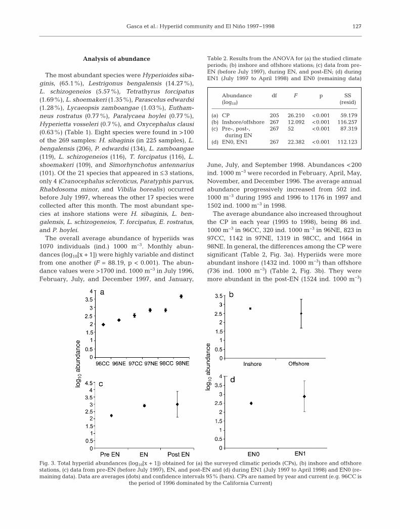
Analysis of abundance

The most abundant species were Hyperioides siba -ginis, (65.1%), Lestrigonus bengalensis (14.27%),L. schizogeneios (5.57%), Tetrathyrus forcipatus(1.69%), L. shoemakeri (1.35%), Parascelus edwardsi(1.28%), Lycaeopsis zamboangae (1.03%), Eutham-neus rostratus (0.77%), Paralycaea hoylei (0.77%),Hyperietta vosseleri (0.7%), and Oxycephalus clausi(0.63%) (Table 1). Eight species were found in >100of the 269 samples: H. sibaginis (in 225 samples), L.bengalensis (206), P. edwardsi (134), L. zamboangae(119), L. schizogeneios (116), T. forcipatus (116), L.shoemakeri (109), and Simorhynchotus antennarius(101). Of the 21 species that appeared in ≤ 3 stations,only 4 (Cranocephalus scleroticus, Paratyphis parvus,Rhabdosoma minor, and Vibilia borealis) occurredbefore July 1997, whereas the other 17 species werecollected after this month. The most abundant spe-cies at inshore stations were H. sibaginis, L. ben-galensis, L. schizogeneios, T. forcipatus, E. rostratus,and P. hoylei.

The overall average abundance of hyperiids was1070 individuals (ind.) 1000 m−3. Monthly abun-dances (log10[x + 1]) were highly variable and distinctfrom one another (F = 88.19, p < 0.001). The abun-dance values were >1700 ind. 1000 m−3 in July 1996,February, July, and December 1997, and January,

June, July, and September 1998. Abundances <200ind. 1000 m−3 were recorded in February, April, May,November, and December 1996. The average annualabundance progressively increased from 502 ind.1000 m−3 during 1995 and 1996 to 1176 in 1997 and1502 ind. 1000 m−3 in 1998.

The average abundance also increased throughoutthe CP in each year (1995 to 1998), being 86 ind.1000 m−3 in 96CC, 320 ind. 1000 m−3 in 96NE, 823 in97CC, 1142 in 97NE, 1319 in 98CC, and 1664 in98NE. In general, the differences among the CP weresignificant (Table 2, Fig. 3a). Hyperiids were moreabundant inshore (1432 ind. 1000 m−3) than offshore(736 ind. 1000 m−3) (Table 2, Fig. 3b). They weremore abundant in the post-EN (1524 ind. 1000 m−3)

127

Abundance df F p SS (log10) (resid)

(a) CP 205 26.210 <0.001 59.179(b) Inshore/offshore 267 12.092 <0.001 116.257(c) Pre-, post-, 267 52 <0.001 87.319 during EN(d) EN0, EN1 267 22.382 <0.001 112.123

Table 2. Results from the ANOVA for (a) the studied climateperiods; (b) inshore and offshore stations; (c) data from pre-EN (before July 1997), during EN, and post-EN; (d) duringEN1 (July 1997 to April 1998) and EN0 (remaining data)

Fig. 3. Total hyperiid abundances (log10[x + 1]) obtained for (a) the surveyed climatic periods (CPs), (b) inshore and offshorestations, (c) data from pre-EN (before July 1997), EN, and post-EN and (d) during EN1 (July 1997 to April 1998) and EN0 (re-maining data). Data are averages (dots) and confidence intervals 95% (bars). CPs are named by year and current (e.g. 96CC is

the period of 1996 dominated by the California Current)

Mar Ecol Prog Ser 455: 123–139, 2012128

Fig. 4. Monthly average abundances (log10[x + 1]) and 95% confidence interval of total numbers of Hyperioides siba ginis,Lestrigonus bengalensis, Lestrigonus schizogeneios, Tetrathyrus forcipatus, Lestrigonus shoemakeri, Parascelus edwardsi,

Lycaeopsis zamboangae, and Hyperietta vosseleri in the studied area. d: inshore stations, J: offshore stations


period than before (594 ind. 1000 m−3) or during theEN (1432 ind. 1000 m−3) (Table 2, Fig. 3c). Further-more, they were also more abundant during theinfluence of EN than in all other samples (914 ind.1000 m−3) (Table 2, Fig. 3d).

The most abundant species were more abundantin shore than offshore. Hyperioides sibaginis had anaverage of 948 ind. 1000 m−3 inshore and 457 ind.1000 m−3 at offshore stations; the same pattern wasob ser ved in Lestrigonus bengalensis (191 vs. 117ind. 1000 m−3), L. schizogeneios (107 vs. 13), Tetra -thyrus forci patus (26 vs. 11), and Parascelus ed -ward si (15 vs. 12).

A significant correlation (F = 4.117, p < 0.1) wasobtained between the monthly geometric mean (GM)of hyperiid abundance and Niño Index 3.4 (SSTindex for the Niño 3.4 Region; Trenberth 1997). Wealso observed a significant relationship between themonthly GM of Hyperioides siba ginis and the sameEN index (F = 2.094, p = 0.163) but not for the GM ofthe other most abundant species, Lestrigonus benga -lensis, (F = 0.177, p = 0.6775). The monthly abun-dances of hyperiid species with average densities>10 ind. 1000 m−3 were plotted to observe the tempo-ral variations (Fig. 4).

Analysis of diversity

Species richness

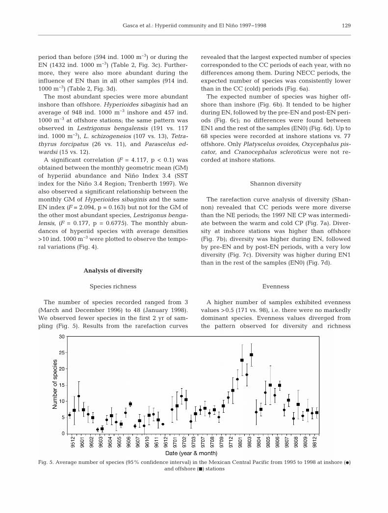
The number of species recorded ranged from 3(March and December 1996) to 48 (January 1998).We observed fewer species in the first 2 yr of sam-pling (Fig. 5). Results from the rarefaction curves

revealed that the largest expected number of speciescorresponded to the CC periods of each year, with nodifferences among them. During NECC periods, theexpected number of species was consistently lowerthan in the CC (cold) periods (Fig. 6a).

The expected number of species was higher off-shore than inshore (Fig. 6b). It tended to be higherduring EN, followed by the pre-EN and post-EN peri-ods (Fig. 6c); no differences were found betweenEN1 and the rest of the samples (EN0) (Fig. 6d). Up to68 species were recorded at inshore stations vs. 77offshore. Only Platyscelus ovoides, Oxycephalus pis-cator, and Cranocephalus scleroticus were not re -corded at inshore stations.

Shannon diversity

The rarefaction curve analysis of diversity (Shan-non) revealed that CC periods were more diversethan the NE periods; the 1997 NE CP was intermedi-ate between the warm and cold CP (Fig. 7a). Diver-sity at inshore stations was higher than offshore(Fig. 7b); diversity was higher during EN, followedby pre-EN and by post-EN periods, with a very lowdiversity (Fig. 7c). Diversity was higher during EN1than in the rest of the samples (EN0) (Fig. 7d).

Evenness

A higher number of samples exhibited evennessvalues >0.5 (171 vs. 98), i.e. there were no markedlydominant species. Evenness values diverged fromthe pattern observed for diversity and richness

129

Fig. 5. Average number of species (95% confidence interval) in the Mexican Central Pacific from 1995 to 1998 at inshore (d) and offshore (j) stations

Mar Ecol Prog Ser 455: 123–139, 2012

(Fig. 8a). Higher values of evenness were found dur-ing the influence of EN and were similar to those of96CC. Extreme values of this index were observed in1996. A reverse tendency occurred in 1997: duringthe NE, values were higher than during the CC, and

evenness was uniform between 97CC and 98NE.Dominance was lower offshore (Fig. 8b), and greaterevenness values occurred during the pre-EN than inthe post-EN period (Fig. 8c). A high evenness wasfound during EN1 than during EN0 (Fig. 8d).

130

Fig. 6. Species richness based on rarefaction curves. (a) Surveyed CPs; (b) inshore and offshore stations; (c) data from pre-EN (before July 1997), EN, and post-EN; (d) during EN 1 (July 1997 to April 1998) and EN 0 (remaining data)

Fig. 7. Shannon diversity based on rarefaction curves. (a) Surveyed CPs; (b) inshore and offshore stations; (c) data from pre-EN (before July 1997), EN, and post-EN; (d) during EN 1 (July 1997 to April 1998) and EN 0 (remaining data)


Community analysis

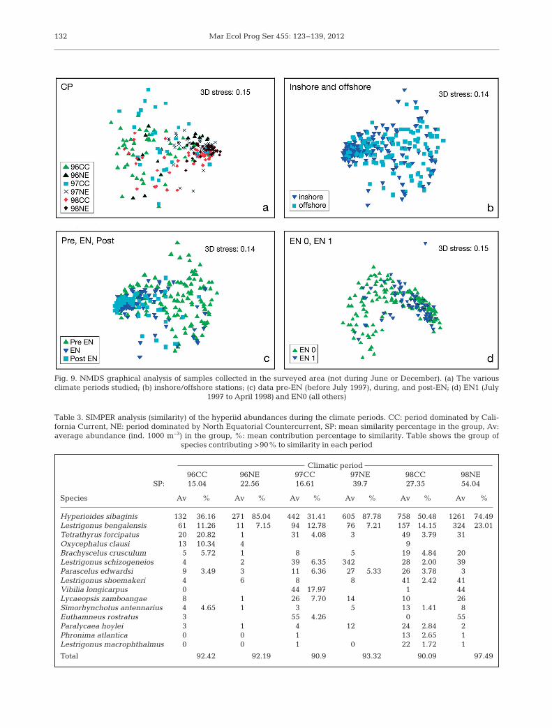
The nMDS applied to CPs, distance to coast, andEN showed an acceptable fit (stress = 0.14) (Clarke& Gorley 2006); however, the large number of sam-ples in a single graphic hampered the visual detec-tion of spatial and temporal patterns (Fig. 9a−d).The ar rangement of the CP (Fig. 9a) shows disper-sion of the samples during the EN influence period.The CP CC group shows a greater similarity. The98CC period reflects the full effect of EN in the areaand was the most compact group. No inshore-off-shore pattern was observed (Fig. 9b), but the pre-EN, EN, and post-EN periods were well defined(Fig. 9c).

The ANOSIM analysis showed significant differ-ences between the CPs (R = 0.226, p < 0.001), amongthe pre-EN, EN, and post-EN samples (R = 0.069,p < 0.001), and also based on the distance from thecoast (R = 0.03, p < 0.001). The ANOSIM betweenEN1 (July 1997 to March 1998) and the rest of sam-ples did not show significant differences (R = −0.102,p = 1.00). For all paired analyses of CP, the differ-ences were significant at p < 0.001 (except for 96CCand 96NE, for which p = 0.019, and for the pair 97CCand 96NE with p = 0.012) (Tables 3 to 6).

The SIMPER analysis shows that during the CCperiods there are more species with low contributionthan in the NE period. During the NE period, Hy peri -oides sibaginis and Lestrigonus bengalensis rep -resented >90% of the similarity within groups(Table 3). Also, H. sibaginis and L. bengalensis dom-inated in all of the studied groups. Other species,such as Tetrathyrus forcipatus, Oxycephalus clausi,Parascelus edwardsi, and L. schizogeneios, contrib -uted mainly to the communities of CC periods(Table 4).

Fewer species contributed to the NE than to the CCcommunity. The last 3 CPs were similar, with highabundance, although their composition differed. Themain feature of CP 98NE, the most dissimilar of theCPs, is that Hyperioides sibaginis and Lestrigonusbengalensis contributed 74.5 and 23.0%, respective -ly, to their community, and together they dominated,forming >97% of the assemblage during that period.L. bengalensis contributed more in this period than inthe other NE periods.

Unlike other CC periods, the 98CC period had aminor relative contribution of Hyperioides sibaginis;a group of species including Brachyscelus crusculum,Tetrathyrus forcipatus, Parascelus edwardsi, Paraly-caea hoylei, Phronima atlantica, and Vibilia armata

131

Fig. 8. Evenness based on rarefaction curves. (a) Surveyed CPs; (b) inshore and offshore stations; (c) data from pre-EN (beforeJuly 1997), EN, and post-EN; (d) during EN 1 (July 1997 to April 1998) and EN 0 (remaining data). PIE: probability of inter-

specific encounter

Mar Ecol Prog Ser 455: 123–139, 2012132

Fig. 9. NMDS graphical analysis of samples collected in the surveyed area (not during June or December). (a) The various climate periods studied; (b) inshore/offshore stations; (c) data pre-EN (before July 1997), during, and post-EN; (d) EN1 (July

1997 to April 1998) and EN0 (all others)

Climatic period96CC 96NE 97CC 97NE 98CC 98NE

SP: 15.04 22.56 16.61 39.7 27.35 54.04

Species Av % Av % Av % Av % Av % Av %

Hyperioides sibaginis 132 36.16 271 85.04 442 31.41 605 87.78 758 50.48 1261 74.49Lestrigonus bengalensis 61 11.26 11 7.15 94 12.78 76 7.21 157 14.15 324 23.01Tetrathyrus forcipatus 20 20.82 1 31 4.08 3 49 3.79 31Oxycephalus clausi 13 10.34 4 9 Brachyscelus crusculum 5 5.72 1 8 5 19 4.84 20Lestrigonus schizogeneios 4 2 39 6.35 342 28 2.00 39Parascelus edwardsi 9 3.49 3 11 6.36 27 5.33 26 3.78 3Lestrigonus shoemakeri 4 6 8 8 41 2.42 41Vibilia longicarpus 0 44 17.97 1 44Lycaeopsis zamboangae 8 1 26 7.70 14 10 26Simorhynchotus antennarius 4 4.65 1 3 5 13 1.41 8Euthamneus rostratus 3 55 4.26 0 55Paralycaea hoylei 3 1 4 12 24 2.84 2Phronima atlantica 0 0 1 13 2.65 1Lestrigonus macrophthalmus 0 0 1 0 22 1.72 1

Total 92.42 92.19 90.9 93.32 90.09 97.49

Table 3. SIMPER analysis (similarity) of the hyperiid abundances during the climate periods. CC: period dominated by Cali -fornia Current, NE: period dominated by North Equatorial Countercurrent, SP: mean similarity percentage in the group, Av:average abundance (ind. 1000 m−3) in the group, %: mean contribution percentage to similarity. Table shows the group of

species contributing >90% to similarity in each period

Gasca et al.: Hyperiid community and El Niño 1997−1998 133

96C

C &

96C

C &

96C

C &

96C

C &

96C

C &

96N

E &

96N

E &

96N

E &

96N

E &

97C

C &

97C

C &

97C

C &

97N

E &

97N

E &

98C

C &

96N

E97

CC

97N

E98

CC

98N

E97

CC

97N

E98

CC

98N

E97

NE

98C

C98

NE

98C

C98

NE

98N

E

DP

:86

.92

88.2

384

.93

87.3

787

.09

86.9

172

.32

82.6

975

.11

81.1

983

.89

81.5

173

.14

60.6

967

.16

R:

0.12

60.

170

0.27

80.

249

0.44

30.

139

0.22

50.

241

0.48

40.

263

0.19

20.

425

0.12

60.

174

0.12

9p

:0.

019

0.00

10.

001

0.00

10.

001

0.01

20.

006

0.00

30.

001

0.00

10.

001

0.00

10.

001

0.00

10.

001

Sp

ecie

s%

%%

%%

%%

%%

%%

%%

%%

Hyp

erio

ides

sib

agin

is49

.95

28.7

958

39.6

466

.23

43.7

560

.85

46.3

466

.02

52.2

739

.41

61.4

150

.46

60.3

358

.26

Les

trig

onu

s b

eng

alen

sis

9.19

10.3

39.

7610

.84

21.1

7.24

8.08

9.46

22.9

78.

229.

3317

.97

9.36

19.5

316

.14

Les

trig

onu

s sc

hiz

ogen

eios

1.78

4.88

6.98

2.18

3.75

7.43

1.85

7.53

3.04

1.84

6.66

6.4

1.53

Tet

rath

yru

s fo

rcip

atu

s4.

86.

042.

174.

721.

253.

563.

822.

34.

31.

522.

942.

4V

ibil

ia l

ong

icar

pu

s12

.22

10.0

71.

16.

275.

743.

55P

aras

celu

s ed

war

dsi

2.31

2.99

4.75

3.02

2.1

4.76

2.62

3.27

2.87

2.26

1.47

Les

trig

onu

s sh

oem

aker

i3.

752.

311.

622.

762.

912.

243.

341.

492.

642.

512.

01L

ycae

opsi

s za

mb

oan

gae

1.34

4.47

2.39

1.85

3.51

2.15

1.39

2.45

2.37

1.46

1.38

0.79

Bra

chys

celu

s cr

usc

ulu

m1.

932.

625.

261.

84.

433.

492.

451.

66P

aral

ycae

a h

oyle

i1.

593.

741.

583.

411.

352.

922.

661.

77E

uth

amn

eus

rost

ratu

s1.

275.

364.

232.

82.

722.

06O

xyce

ph

alu

s cl

ausi

4.44

3.17

1.93

2.25

0.96

0.93

Hyp

erie

tta

voss

e2.

212.

332.

080.

852.

11.

90.

82L

estr

igon

us

mac

rop

hth

alm

us

1.43

1.43

1.42

1.52

1.26

1.23

1.24

1.6

Lyc

aea

pu

lex

2.55

1.15

1.15

1.68

1.41

1.2

0.81

Vib

ilia

arm

ata

1.55

2.36

2.24

1.56

1.11

Sim

orh

ynch

otu

s an

ten

nar

ius

2.03

1.44

1.41

1.11

0.96

0.94

Ph

ron

ima

atla

nti

ca2.

151.

871.

51.

220.

89L

ycae

a vi

nce

nti

i1.

441.

350.

911.

381.

021.

05L

ycae

opsi

s th

emis

toid

es1.

521.

581.

221.

06P

laty

scel

us

serr

atu

lus

1.12

0.89

0.74

0.75

0.78

Sci

na

mar

gin

ata

1.64

1.3

0.78

Rh

abd

osom

a w

hit

ei1.

372.

16L

ycae

a p

ach

ypod

a1.

191.

48V

ibil

ia p

rop

inq

ua

0.9

0.99

0.7

Lyc

aea

serr

ata

1.19

0.96

Am

ph

ith

yru

s sc

ulp

tura

tus

0.96

0.74

Vib

ilia

bor

eali

s 1.

17

90.8

791

.13

91.3

890

.18

90.0

290

.67

90.5

390

.190

.51

90.0

390

.68

91.0

490

.53

90.4

390

.13

Tab

le 4

. S

IMP

ER

an

alys

is (

dis

sim

ilar

ity)

of

the

hyp

erii

d s

pec

ies

abu

nd

ance

s d

uri

ng

th

e cl

imat

e p

erio

ds.

DP

: m

ean

dis

sim

ilar

ity

per

cen

tag

e fo

r ea

ch g

rou

p,

R:

resu

lts

of t

he

AN

OS

IM t

est

of p

aire

d c

omp

aris

ons,

p:

asso

ciat

ed p

rob

abil

ity,

%:

mea

n c

ontr

ibu

tion

per

cen

tag

e to

dis

sim

ilar

ity.

CC

: p

erio

d d

omin

ated

by

Cal

ifor

nia

Cu

rren

t,

NE

: per

iod

dom

inat

ed b

y N

orth

Eq

uat

oria

l Cou

nte

rcu

rren

t

Mar Ecol Prog Ser 455: 123–139, 2012

was related to the peak of EN influence (ca. January1998) (Table 4).

Hyperioides sibaginis and Lestrigonus bengalensiscontributed up to 93% of the similarity during thepost-EN period (Table 5). In the pre-EN group,besides H. sibaginis, other species (Tetrathyrus forci-patus, Oxycephalus clausi, Parascelus edwardsi,Brachyscelus crusculum, Lestrigonus schizogeneios,and Euthamneus rostratus) marked the group. Dur-ing EN, P. edwardsi, L. shoemakeri, and L. schizo-geneios, in addition to the 2 most abundant species,contributed >90% to the group. The EN and post-ENgroups were the least dissimilar, but the greaterdominance of H. sibaginis and L. bengalensis and ahigher number of species in the post-EN group werethe main differences (Table 5).

Up to 90% of the group at the inshore stations wasrepresented by Hyperioides sibaginis, Lestrigonusbengalensis, and Tetrathyrus forcipatus; the offshoregroup included the first 2 species as well (Table 6).The dissimilarity analysis showed that the maininshore-offshore difference is that these species areless abundant off the coast.

The redundancy analysis showed 2 almost orthogo-nal axes representing the temporal variation de finedby the multivariable El Niño Index (MEI) and the spa-

tial variation defined by the distance of the stationson the coast (Fig. 10). Zooplankton biomass showed ahigh correlation with the axis of distance from shore.The species associated with EN (high MEI values)were Eupronoe armata, Lycaeopsis themistoides,Am phi thyrus sculpturatus, Lestrigonus shoemakeri,Phro nimella elongata, Hyperietta vosse leri, and Phro -nima atlantica. The species related to low MEI valueswere Lycaea pachypoda, Crano cephalus scleroticus,and Rhabdosoma minor. Both of the patterns of vari-ability, the inter-annual related to the EN event andthe seasonal one, were detected (Fig. 10). The groupof stations during the EN period was more compactthan in the pre-EN period. The greater dispersion ofstations on the vertical axis shown during CC periodssuggests a warm-cold periodic variability, which wasweak but detectable during 98CC (EN). The MonteCarlo method indicates a significant relationship withenvironmental variables (Table 6).

DISCUSSION

The search for understanding of the functionalstructure of the pelagic ecosystem is currently at thecore of modern oceanography. This structure is de -

134

Similarity Dissimilarity Pre- EN Post- Pre- & Pre- & EN & EN EN EN post-EN post-EN

SA/DA: 15.01 32.72 38.54 82.1 82.12 65.9R: 0.09 0.109 0.017p: 0.001 0.002 0.014

Species Av (%) Av (%) Av (%)

Hyperioides sibaginis 394 51.26 880 74.4 1041 67.24 52.54 55.37 55.44Lestrigonus bengalensis 70 15.49 139 11.33 342 25.81 10.36 19.5 16.52Tetrathyrus forcipatus 18 7.81 28 7 3.11 1.83 1.92Oxycephalus clausi 9 4.65 8 0 1.47 0.95 Brachyscelus crusculum 5 3.44 11 3 2.54 1.29Lestrigonus schizogeneios 13 2.59 167 1.53 9 4.4 1.52 3.78Parascelus edwardsi 10 3.73 25 3.91 7 3.12 1.37 1.98Lestrigonus shoemakeri 6 29 1.66 11 2.5 1.67 2.07Vibilia longicarpus 12 3 0 1.8 1.2 Lycaeopsis zamboangae 11 10 13 1.63 1.86 1.21Simorhynchotus antennarius 3 9 8 0.91 0.78Euthamneus rostratus 17 1.91 2 1.06 1.44 Paralycaea hoylei 11 15 1.27 1.95 1.83Lestrigonus macrophthalmus 10 13 1.4 1.35Hyperietta vosseleri 19 4 1.7 1.42

Total 90.87 90.87 93.05 88.4 90.05 89.59

Table 5. SIMPER analysis (similarity and dissimilarity) of the hyperiid species abundances during pre-EN (before July 1997),EN (July 1997 to April 1998), and post-EN periods. Av: average abundance of group, SA: similarity average, DA: dissimilarity

average, R: ANOSIM test of paired comparisons, p: associated probability, %: contribution to group


termined by physical forces and theassociated biological responses (Platt& Sathyendranath 1999). Our analysisprovides evidence showing that thelocal hyperiid community structurehas distinctive features according todistinct hydrographic patterns. It alsoreveals that these patterns are differ-ent from those observed in surround-ing areas and diverge from thoseknown for other zooplanktonic taxa.

Species composition

Previous studies of the hyperiids ofMexico’s central Pacific are scarce(Gasca & Franco-Gordo 2008). It wasexpected that the monthly collectionof samples for 2 yr (1996 to July 1997)would provide a complete account ofspecies in the area. We did not expectthe additional increase of speciesobserved after July 1997 in the surveyed area. Theaddition of almost 30% of the previous species rich-ness indicates that hyperiids, like other zooplankton,show a sharp increase of tropical-equatorial formsduring EN, as was observed for copepods (Lavanie-gos et al. 2003, Palomares-García et al. 2003, López-Ibarra & Palomares-García 2006) and salps (Hereu et

al. 2006). Furthermore, considering the 56 speciesknown before the onset of EN and the 24 recordedafter July 1997, the increase was 43% (Table 2)(Gasca 2009a, Gasca et al. 2010).

The 84 species recognized in tropical areas of thePacific coast of Mexico, south of Baja California, i.e.80 in this study plus Vibilia pyripes, V. australis, V.

cultri pes, and V. stebbingi, recordedby Shih & Hen drycks (2003), repre-sent ~50% of all known species in thetropical Pacific (Vinogradov 1991).This figure is comparable to that ofother subregions of the Pacific (Vino-gradov 1991: 119 species; Shulen-berger 1977: 83 species). However,>200 species have been found tooccur in the Pacific Ocean (Shih &Cheng 1995, Vinogradov et al. 1996),and regional lists should grow whendeeper waters are sampled (Gasca2009b).

Abundance

A group of species including Phron-ima atlantica, Phronimella elongata,Phrosina semilunata, and some spe-cies of Primno was proposed by Vino-gradov (1999) as being among the

135

Similarity Dissimilarity Inshore Offshore Inshore vs. offshore

SA/DA (%) 24.43 21.11 78.21

Av % Av %

Hyperioides sibaginis 948 73.39 458 58.14 51.75Lestrigonus bengalensis 191 14.66 117 19.94 13.79Tetrathyrus forcipatus 26 3.06 11 3.26Oxycephalus clausi 9 5 1.78Brachyscelus crusculum 7 6 2.09 1.8Lestrigonus schizogeneios 108 13 2.49 3.51Parascelus edwardsi 15 13 3.44 2.31Lestrigonus shoemakeri 12 17 2.17 2.21Vibilia longicarpus 7 5 2.12Lycaeopsis zamboangae 10 12 2.68 1.73Euthamneus rostratus 13 3 1.55

Total 91.11 90.95 85.81

Table 6. SIMPER analysis (similarity and dissimilarity) of the hyperiid speciesabundances at inshore and offshore stations during the surveyed period. Av:average abundance of group, %: contribution to group, SA: similarity average,

DA: dissimilarity average

Fig. 10. Ordination pattern of temporal variation from the redundancy analysis

Mar Ecol Prog Ser 455: 123–139, 2012

most abundant species in the Pacific. However, datafrom different regions, such as the eastern SouthPacific Gyre (Vinogradov 1991), the Gulf of Califor-nia (Siegel-Causey 1982) and the CC area off BajaCalifornia (Lavaniegos & Hereu 2009), suggest a dif-ferent trend. In the study area and in other tropicalPacific regions, Hyperioides sibaginis and Lestri -gonus bengalensis were the most abundant (Gasca &Franco-Gordo 2008, Zeidler 1984, Valencia & Giraldo2009). In general, each area of the Eastern Pacificwith different oceanographic features can be charac-terized by a defined group of most abundant species.

The hyperiid fauna of the Mexican tropical Pacificresembles that of the Gulf of California but clearlydiffers from that of the CC. None of the 4 most com-mon species in the surveyed area are among the pre-dominant forms in the California region (Brusca1981, Lavaniegos & Ohman 1999). This suggests thatthe presumed CC influence was not detected in thelocal hyperiid fauna even during the CC periods.However, the increase in the number of species inthe CC periods shows the arrival of species fromother subregions.

The overall average abundance of hyperiids in thestudy area (1070 ind. 1000 m−3) was similar to thatfound in the adjacent Banderas Bay (1167 ind.1000 m−3 in September) (Gasca & Franco-Gordo2008) and is comparable to values reported in otherareas, like the North Pacific Central Gyre (1 to 3695ind. 400 m−3) or adjacent areas of the Atlantic such asthe Gulf of Mexico (1437 ind. 1000 m−3) (Gasca 2004),but is higher than those found in oligotrophic watersof the Caribbean (240 ind. 1000 m−3) (Gasca & Suá -rez-Morales 2004).

Hyperiid abundance was relatively low during1996, and the local community structure was charac-terized by the dominance of Hyperioides sibaginisand Lestrigonus bengalensis. The progressive in -crease in the abundance of hyperiids from the begin-ning to the end of the sampling period, as shown bythe average of the different CP (Fig. 2a), was unex-pected. It is possible that it resulted from the additionof populations of different origins or the influence ofEN. The influence of the cold (CC) and warm (NE)conditions in the area was clear, with lower abun-dances during the cold periods than in the warmones, a pattern that remained even during the ENyear. The only CPs in which no differences in abun-dance occurred were 97NE and 98CC, both duringEN. Hence, the hyperiid abundance could be consid-ered as a local indicator of EN. Furthermore, evengreater abundances were recorded in the followingmonths, suggesting that EN may trigger or favor

higher reproductive rates of the dominant species fora longer period.

Quite unexpectedly, hyperiids were more abun-dant during the EN than during the previous years.EN has been commonly associated with a relativelylow zooplankton productivity and abundance (Bar-ber & Chavez 1983, Roemmich & McGowan 1995,Franco-Gordo et al. 2001a,b, 2004). Locally, this ef fect could be explained by an increase in the repro-duction of the dominant hyperiid species and possi-bly by the addition of populations of different originsresulting from the local convergence of distinct watermasses.

The 4 most abundant species in this study (Hyperi-oides sibaginis, Lestrigonus bengalensis, L. schizo-geneios, and Tetrathyrus forcipatus) were the samethroughout the study period. The other speciesshowed 2 patterns: (1) occurring or being more fre-quent during EN (e.g. Paralycaea gracilis, Eupronoearmata, Anchylomera blossevillei, and Phronimellaelongata) and (2) absent or decreasing in frequencyduring EN (e.g. Scina marginata, T. forcipatus,Crano cephalus scleroticus, Rhabdosoma minor, andLycaea pachypoda); these species were also absentwhen warm waters prevailed in the area.

Diversity

Sequential changes in richness were evident andrelated to the arrival of warmer waters (PESW) result-ing from the influence of EN. The number of specieswas significantly lower during the first half of thestudy than in the second (Fig. 5). During the study pe-riod, the temporal monitoring of the species richnessallowed the detection of changes that may be associ-ated with variations of the hydrographic conditions.Unexpectedly, richness values in the CC CPs werehigher than during the warm (NE) periods, but aneven greater richness value was recorded in CC 1998;this could be due to the addition of the PEW fauna ar-riving with EN. Lavaniegos & Ohman (1999) observeda different pattern in the CC off southern California;they observed that the years with fewer species were1995 and 1997, although in 1972 (an other EN year),they also recorded more species. The finding ofgreater richness during EN (vs. pre- and post-EN) andEN-related CPs indicates the strong influences of thisevent on the expected number of species.

Greater diversity values in CC than in NECC peri-ods are explained by the combination of the follow-ing factors: (1) the high number of species found inCP CC, (2) their low dominance, (3) the arrival of

136


water from the north and east adding to the localfauna, and (4) reduced dominance of the 2 mostabundant species in the area. The greater diversityobserved in the 97NE period resulted from a higherevenness value. The high diversity found in EN1 isrelated to the higher number of species found in thatperiod. In contrast, the post-EN low diversity resultsfrom the high dominance of Hyperioides sibaginisand Lestrigonus bengalensis in that period; thesespecies were favored by the warm conditions associ-ated with EN.

Evenness

The mixing of water masses during the CC and ENperiods was favorable for higher values of evennessand characterized the convergence of waters in thearea. The arrival of warm water fauna weakened thedominance of some species, as observed in otherNECC periods. That is, at the onset of EN, the NECChyperiid community is more similar to that influ-enced by the CC influence (with higher diversity andlower dominance).

Analysis of the hyperiid community

The ANOSIM revealed CP- and EN-related com-munities and also inshore and offshore communitiesin an area where the continental shelf is very narrow.There is a defined community structure related to EN(EN1: July 1997 to March 1998). The SIMPER analy-sis allowed us to define the structure of each of thecommunities tested (Tables 3 to 6).

As found in our survey, the known biological con-sequences of EN in the zooplankton include changesin species composition (Gómez-Gutiérrez et al. 1995,González et al. 2000, Lavaniegos & Ohman 1999).Also, biomass may increase (Brodeur & Ware 1992),decrease (Roemmich & McGowan 1995), or remainstable (Lavaniegos & Ohman 1999), depending onthe area and the group surveyed (Fiedler 2002). Theimpoverishment of the pelagic environment as aneffect of EN has also been described for zooplanktonand ichthyoplankton taxa in the eastern Pacific(Chavez et al. 1999, Franco-Gordo et al. 2004); how-ever, the local hyperiid community showed a reversepattern (e.g. higher abundances and diversity). Thismay be related to the biology of some of the speciesthat use other organisms (gelatinous zooplankton) fortheir sustainment and thus do not depend entirely onthe availability of food in the environment.

Franco-Gordo et al. (2004) found local inter-annualvariations of the zooplankton biomass and the ichthy-oplankton related to EN (e.g. less abundance anddiversity). They also detected a response of the fishlarvae community to seasonal cycles related tohydrographic and climatic conditions. As reportedherein, hyperiids showed a seasonal variation result-ing from the influence of EN, but with an oppositepattern. Under the influence of the CC, fish larvaeand biomass showed a greater abundance and areduced diversity and evenness, whereas during EN,the abundance and diversity were lower.

During the onset of EN, the biological productionand dynamics changed in coastal areas of the CCsystem and other areas of the Eastern Tropical Pacific(Morales-Ramírez & Brugnoli-Olivera 2001, Lavanie-gos et al. 2002). Conditions returned to normality inthe aftermath. A similar response, with a delay of 1 to2 mo, was observed in the tropical Pacific (Chavez etal. 1998, 1999), suggesting that the influence of EN inthe regional biota is detectable at the initial but not atthe final stages. This is true for the local hyperiidcommunity, whose return to pre-EN conditions wasnot observed. Our results suggest that the residualeffects of EN on the hyperiid community continuedfor several months after the oceanographic end ofEN. This inertial response has not been describedpreviously and is evidence of the wide variety ofpotential responses that different zooplankton taxamay present as part of this complex pelagic commu-nity. It is necessary to study the biological-physicalcoupling of different zooplankton groups in the areaduring EN to fully understand the effects of this eventin the community.

Acknowledgements. This work is part of the doctoral thesispresented by R.G. in the postgraduate program of the Uni-versidad de Guadalajara. Funding for fieldwork and generallogistic support was provided by CUCSUR, Universidad deGuadalajara. We thank the crew of the R/V ‘BIP-V’ for theirhelp and guidance during these years of sampling. We re -ceived assistance from numerous persons in the many yearsof fieldwork; we sincerely thank them all. G. González-San-són provided useful comments to improve the statisticalanalyses presented in this work. A database of the informa-tion presented herein was prepared with the aid ofCONABIO project DJo24.

LITERATURE CITED

Aguirre-Gómez R, Salmerón O, Álvarez R (2003) Effects ofENSO off the southwest coast of Mexico, 1996–1999.Geofis Int 42: 377−388

Badán-Dangón ARF (2003) The effects of El Niño in Mexico: a survey. Geofís Int 42: 1−3

Barber RT, Chavez FP (1983) Biological consequences of ElNiño. Science 222: 1203−1210

137

Mar Ecol Prog Ser 455: 123–139, 2012

Bary BM (1959a) Species of zooplankton as a means of iden-tifying different surface waters and demonstrating theirmovements and mixing. Pac Sci 13: 14−54

Bary BM (1959b) Ecology and distribution of some pelagicHyperiidea (Crustacea: Amphipoda) from New Zealandwaters. Pac Sci 13: 317−334

Brodeur RD, Ware DM (1992) Long-term variability in zoo-plankton biomass in the subarctic Pacific Ocean. FishOceanogr 1: 32−38

Brusca GJ (1967) The ecology of pelagic amphipods. I. Spe-cies accounts, vertical zonation and migration of amphi -pods from the waters off southern California. Pac Sci 21: 382−393

Brusca GJ (1981) Annotated keys to the Hyperiidea (Crus-tacea: Amphipoda) of North American coastal waters.Allan Hancock Found Tech Rep 5: 1−76

Brusca RC, Hendrickx ME (2005) Crustacea 4. Peracarida: Lophogastrida, Mysida, Amphipoda, Tanaidacea andCumacea. In: Hendrickx ME, Brusca RC, Findley LT(eds) A distributional checklist of the macrofauna of theGulf of California, Mexico. Part I. Invertebrates. Arizona-Sonora Desert Museum, Tucson, AZ, p 147−154

Chavez FP, Strutton PG, McPhaden MJ (1998) Biological-physical coupling in the central equatorial Pacific duringthe onset of the 1997-98 El Niño. Geophys Res Lett 25: 3543−3546

Chavez FP, Strutton PG, Friederich GE, Feely RA, FeldmanGC, Foley DG, McPhaden MJ (1999) Biological andchemical response of the equatorial Pacific Ocean to the1997−98 El Niño. Science 286: 2126−2131

Clarke KR (1993) Non-parametric multivariate analyses ofchanges in community structure. Aust J Ecol 18: 117−143

Clarke KR, Gorley RN (2006) PRIMER v6: user manual/tuto-rial. PRIMER-E, Plymouth

Clarke KR, Warwick RM (2001) Change in marine commu-nities: an approach to statistical analysis and interpreta-tion, 2nd edn. PRIMER-E, Plymouth

Clarke KR, Somerfield PJ, Chapman MG (2006) On resem-blance measures for ecological studies, including taxo-nomic dissimilarities and zero-adjusted Bray-Curtis coef-ficient for denuded assemblages. J Exp Mar Biol Ecol330: 55−80

Fiedler PC (2002) Environmental change in the eastern trop-ical Pacific Ocean: review of ENSO and decadal variabil-ity. Mar Ecol Prog Ser 244: 265−283

Filonov A, Tereshchenko I (2000) El Niño 1997−98 monitor-ing in mixed layer at the Pacific Ocean near Mexico’swest coast. Geophys Res Lett 27: 705−707

Filonov A, Tereshchenko IE (2010) El régimen termod-inámico en la costa de los estados de Jalisco y Colima. In: Godínez-Domínguez E, Franco-Gordo MC, Rojo-Váz -quez JA, Silva-Bátiz FA, González Sansón G (eds) Eco-sistemas marinos de la Costa Sur de Jalisco y ColimaUniversidad de Guadalajara, Autlán de Navarro, Méx-ico, p 29−72

Franco-Gordo C, Godínez-Domínguez E, Suárez-Morales E(2001a) Zooplankton biomass variability in the MexicanEastern Tropical Pacific. Pac Sci 55: 191−202

Franco-Gordo C, Suárez-Morales E, Godínez-Domínguez E,Flores R (2001b) A seasonal survey of the fish larvaecommunity of the central Pacific coast of Mexico. BullMar Sci 68: 383−396

Franco-Gordo C, Godínez-Domínguez E, Filonov AE,Tereshchenko IE, Freire J (2004) Plankton biomass andlarval fish abundance prior to and during the El Niño

period of 1997–1998 along the Central Pacific coast ofMéxico. Prog Oceanogr 63: 99−123

Gasca R (2004) Distribution and abundance of hyperiidamphipods in relation to summer mesoscale features inthe southern Gulf of Mexico. J Plankton Res 26: 993−1003

Gasca R (2009a) Hyperiid amphipods (Crustacea: Pera -carida) in Mexican waters of the Pacific Ocean. Pac Sci63: 83−95

Gasca R (2009b) Diversity of hyperiid amphipods (Crusta -cea: Peracarida) in the Western Caribbean Sea: newsfrom the deep. Zool Stud 48: 63−70

Gasca R, Franco-Gordo C (2008) Hyperiid amphipods (Per-acarida) from Banderas Bay, Mexican Tropical Pacific.Crustaceana 81: 563−575

Gasca R, Haddock SHD (2004) Associations between gelati-nous zooplankton and hyperiid amphipods (Crustacea: Peracarida) in the Gulf of California. Hydrobiologia530−531: 529−535

Gasca R, Suárez-Morales E (2004) Distribution and abun-dance of hyperiid amphipods (Crustacea: Peracarida)from the Mexican Caribbean Sea, (August 1986). CaribbJ Sci 40: 23−30

Gasca R, Suárez-Morales E, Franco-Gordo C (2010) Newrecords of hyperiids (Amphipoda, Hyperiidea) from sur-face waters of the central Mexican Pacific. Crustaceana83: 927−940

Gómez-Gutiérrez J, Palomares-García R, Gendron D (1995)Community structure of the euphausiid populationsalong the west coast of Baja California, Mexico, duringthe weak ENSO 1986−1987. Mar Ecol Prog Ser 120: 41−51

González HE, Sobarzo M, Figueroa D, Nöthig EM (2000)Composition, biomass and potential grazing impact ofthe crustacean and pelagic tunicates in the northernHumboldt Current area off Chile: differences between ElNiño and non-El Niño years. Mar Ecol Prog Ser 195: 201−220

Gotelli NJ, Entsminger GL (2009) EcoSim: null modellingsoftware for ecologists, Version 7. Acquired Intelligence& Kesey-Bear, Jericho, VT, http: //garyentsminger.com/ecosim/

Gotelli NJ, Graves GR (1996) Null models in ecology. Smith-sonian Institution Press, Washington DC

Harbison GR, Madin LP (1976) Description of the femaleLycaea nasuta Claus, 1879 with an illustrated key to thespecies of Lycaea Dana, 1852 (Amphipoda, Hyperiidea).Bull Mar Sci 26: 165−171

Hereu CM, Lavaniegos BE, Gaxiola-Castro G, Ohman MD(2006) Composition and potential grazing impact of salpassemblages off Baja California during the 1997−1999 ElNiño and La Niña. Mar Ecol Prog Ser 318: 123−140

Hurlbert SH (1971) The nonconcept of species diversity: acritique and alternative parameters. Ecology 52: 577−585

Kane JE (1962) Amphipoda from waters south of NewZealand. N Z J Sci 5: 295−310

Kessler WS (2006) The circulation of the Eastern TropicalPacific: a review. Prog Oceanogr 69: 181−217

Lavaniegos BE, Hereu C (2009) Seasonal variation in hyper-iid amphipod abundance and diversity and influence ofmesoscale structures off Baja California. Mar Ecol ProgSer 394: 137−152

Lavaniegos BE, Ohman MD (1999) Hyperiid amphipods asindicators of climate change in the California Current. In: Schram FR, von Vaupel Klein JC (eds) Crustaceans andthe biodiversity crisis. Proc 4th Int Crustacean Congress.Brill, Leiden, p 489−509

138


Lavaniegos BE, Jiménez-Pérez LC, Gaxiola-Castro G (2002)Plankton response to El Niño 1997-1998 and La Niña1999 in the southern region of the California Current.Prog Oceanogr 54: 33−58

Lavaniegos BE, Gaxiola-Castro G, Jiménez-Pérez LC,González-Esparza MR, Baumgartner T, García-CórdovaJ (2003) 1997-98 El Niño effects on the pelagic ecosystemof the California current off Baja California, Mexico.Geofís Int 42: 483−494

Leps J, Smilauer P (2007) Multivariate analysis of ecologicaldata using CANOCO. Cambridge University Press,Cambridge

Longhurst AR (2006) Ecological geography of the sea, 2ndedn. Elsevier, Amsterdam

López-Ibarra GA, Palomares-García R (2006) Estructura dela comunidad de copépodos en Bahía Magdalena, Méx-ico, durante El Niño 1997–1998. Rev Biol Mar Oceanogr41: 63−76

Marinovic BB, Croll DA, Gong N, Benson SR, Chavez FP(2002) Effects of the 1997–1999 El Nino and La Ninaevents on zooplankton abundance and euphausiid com-munity composition within the Monterey Bay coastalupwelling system. Prog Oceanogr 54: 265−277

Morales-Ramírez A, Brugnoli-Olivera E (2001) El Niño 1997-1998 impact on the plankton dynamics in the Gulf ofNicoya, Pacific coast of Costa Rica. Rev Biol Trop 49: 103−114

Palomares-García R, Martínez-López A, De Silva-Dávila R,Funes-Rodríguez R and others (2003) Biological effects ofEl Niño 1997-98 on a shallow subtropical ecosystem: Bahía Magdalena, Mexico. Geofis Int 42: 455−466

Peterson WT, Keister JE (2002) The effect of a large cape ondistribution patterns of coastal and oceanic copepods offOregon and northern California during the 1998–1999 ElNiño-La Niña. Prog Oceanogr 53: 389−411

Platt T, Sathyendranath S (1999) Spatial structure of pelagicecosystem processes in the global ocean. Ecosystems 2: 384−394

Roemmich D, McGowan J (1995) Climatic warming and thedecline of zooplankton in the California Current. Science267: 1324−1326

Shih Ct (1991) Description of two new species of PhronimaLatreille, 1802 (Amphipoda: Hyperiidea) with a key to allspecies of the genus. J Crustac Biol 11: 322−335

Shih Ct, Cheng Qc (1995) Zooplankton of China seas (2).The Hyperiidea (Crustacea: Amphipoda). China OceanPress, Beijing

Shih Ct, Hendrycks EA (2003) A new species and newrecords of the genus Vibilia Milne Edwards, 1830(amphipoda: Hyperiidea: Vibiliidae) occurring in theeastern Pacific Ocean. J Nat Hist 37: 253−296

Shulenberger E (1977) Hyperiid amphipods from the zoo-

plankton community of the North Pacific central gyre.Mar Biol 42: 375−385

Siegel-Causey D (1982) Factors determining the distributionof hyperiid Amphipoda in the Gulf of California. PhD dis-sertation, University of Arizona, Tucson

Smith PE, Richardson SL (1977) Standard techniques forpelagic fish egg and larvae surveys. FAO Fish Tech Pap175

Sokal RR, Rohlf FJ (1995) Biometry, 3rd edn. Freeman, NewYork, NY

ter Braak CJF, Smilauer P (1998) CANOCO reference man-ual and user’s guide to CANOCO for windows: softwarefor canonical community ordination (version 4). Micro-computer Power, Ithaca, New York, NY

Trasviña A, Barton ED (2008) Summer circulation in theMexican tropical Pacific. Deep-Sea Res I 55: 587−607

Trasviña A, Lluch-Cota D, Filonov AE, Gallegos A (1999)Oceanografía y El Niño. In: Magaña V (ed) Los impactosdel Niño en México. Cap 3, UNAM, México, p 69–101

Trenberth KE (1997) The definition of El Niño. Bull AmMeteorol Soc 78: 2771−2777

Valencia B, Giraldo A (2009) Hipéridos (Crustacea: Amphi -poda) en el sector norte del Pacífico oriental tropicalcolombiano. Lat Am J Aquat Res 37: 265−273 (in Spanishwith English abstract)

Vinogradov GM (1991) Hyperiid amphipods in the easternpart of the South Pacific gyre. Mar Biol 109: 259−265

Vinogradov GM (1999) Amphipoda. In: Boltovskoy D (ed)South Atlantic zooplankton. Backhuys Publishers, Lei-den, p 1141−1240

Vinogradov ME, Volkov AF, Semenova TN (1996) Hyperiidamphipods (Amphipoda, Hyperiidea) of the worldoceans. Science Publishers, Lebanon, NH

Wolter K, Timlin MS (1998) Measuring the strength of ENSOevents: How does 1997–1998 rank? Weather 153: 315−324

Zeidler W (1984) Distribution and abundance of some Hy -per iidea (Crustacea: Amphipoda) in Northern Queens -land waters. Aust J Mar Freshwater Res 35: 285−305

Zeidler W (2003) A review of the hyperiidean amphipodsuperfamily Vibilioidea Bowman and Gruner, 1973(Crusta cea: Amphipoda: Hyperiidea). Zootaxa 280: 1−104

Zeidler W (2004a) A review of the hyperiidean amphipodsuperfamily Lycaepsoidea Bowman and Gruner, 1973(Crustacea: Amphipoda: Hyperiidea). Zootaxa 520: 1−184

Zeidler W (2004b) A review of the families and genera of thehyperiidean amphipod superfamily Phronimoidea Bow-man and Gruner, 1973 (Crustacea: Amphipoda: Hyperi-idea). Zootaxa 567: 1−66

Zeidler W (2006) A review of the hyperiidean amphipodsuperfamily Archaeoscinoidea Vinogradov, Volkov andSemenova, 1982 (Crustacea: Amphipoda: Hyperiidea).Zootaxa 1125: 1−37

139

Editorial responsibility: Hans Heinrich Janssen,Oldendorf/Luhe, Germany

Submitted: September 27, 2011; Accepted: December 21, 2011Proofs received from author(s): May 15, 2012

hyperiid amphipod community in the eastern tropical ... · 2centro universitario de la costa sur...

Documents