i. 2d dft and applications
TRANSCRIPT

Digital Image Processing, 3rd ed. & 2nd ed.
www.ImageProcessingPlace.com
© 1992–2008 R. C. Gonzalez & R. E. Woods
Gonzalez & Woods
DIP Week 3 –part I (largely based on Chapter 4)
I. 2D DFT and Applications
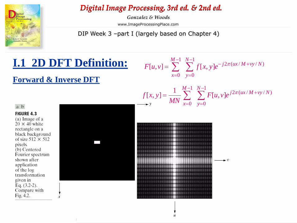
I.1 2D DFT Definitions
I.2 Properties
I.3 Filtering in Frequency Domain
Appendixes (Fourier series, Fourier
transform, FT of sampled signal and
discrete Fourier transform)
Digital Image Processing, 3rd ed. & 2nd ed.
www.ImageProcessingPlace.com
© 1992–2008 R. C. Gonzalez & R. E. Woods
Gonzalez & Woods
DIP Week 3 –part I (largely based on Chapter 4)
1 12 ( / / )
0 0
[ , ] [ , ]M N
j ux M vy N
x y
F u v f x y e
1 12 ( / / )
0 0
1[ , ] [ , ]
M Nj ux M vy N
x y
f x y F u v eMN
I.1 2D DFT Definition:
Forward & Inverse DFT

Digital Image Processing, 3rd ed. & 2nd ed.
www.ImageProcessingPlace.com
© 1992–2008 R. C. Gonzalez & R. E. Woods
Gonzalez & Woods
DIP Week 3 –part I (largely based on Chapter 4)
% create a 512x512 image of black with centre 20x40 white
x=zeros(512,512);
for i=1:20
for j=1:40
x(256-10+i,256-20+j)=255;
end
end
% display the image
figure(1); imshow(x);
% simple 2D DFT
figure(2); y=fft2(x);
% display the DFT magnitude image
imshow(abs(y)/max(max(abs(y))));
% display shifted DFT magnitude image
figure(3); y=fftshift(fft2(x));
imshow(abs(y)/max(max(abs(y))));
% display log magnitude (shifted) DFT magnitude iamge
figure(4); imshow(log(abs(y)),[]); colormap(gray);
Recreate this 2D DFT example in Matlab:

Digital Image Processing, 3rd ed. & 2nd ed.
www.ImageProcessingPlace.com
© 1992–2008 R. C. Gonzalez & R. E. Woods
Gonzalez & Woods
DIP Week 3 –part I (largely based on Chapter 4)

Digital Image Processing, 3rd ed. & 2nd ed.
www.ImageProcessingPlace.com
© 1992–2008 R. C. Gonzalez & R. E. Woods
Gonzalez & Woods
DIP Week 3 –part I (largely based on Chapter 4)

Digital Image Processing, 3rd ed. & 2nd ed.
www.ImageProcessingPlace.com
© 1992–2008 R. C. Gonzalez & R. E. Woods
Gonzalez & Woods
DIP Week 3 –part I (largely based on Chapter 4)
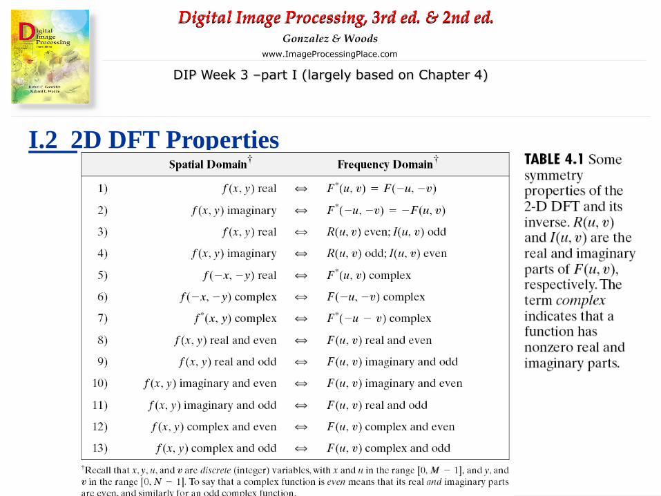
I.2 2D DFT Properties

Digital Image Processing, 3rd ed. & 2nd ed.
www.ImageProcessingPlace.com
© 1992–2008 R. C. Gonzalez & R. E. Woods
Gonzalez & Woods
DIP Week 3 –part I (largely based on Chapter 4)
I.2 2D DFT Properties

Digital Image Processing, 3rd ed. & 2nd ed.
www.ImageProcessingPlace.com
© 1992–2008 R. C. Gonzalez & R. E. Woods
Gonzalez & Woods
DIP Week 3 –part I (largely based on Chapter 4)
I.2 2D DFT Properties
Digital Image Processing, 3rd ed. & 2nd ed.
www.ImageProcessingPlace.com
© 1992–2008 R. C. Gonzalez & R. E. Woods
Gonzalez & Woods
DIP Week 3 –part I (largely based on Chapter 4)
I.2 2D DFT Properties

Digital Image Processing, 3rd ed. & 2nd ed.
www.ImageProcessingPlace.com
© 1992–2008 R. C. Gonzalez & R. E. Woods
Gonzalez & Woods
DIP Week 3 –part I (largely based on Chapter 4)
I.3 Filtering in Frequency Domain
2-Dimensional DFT
& Inverse

Digital Image Processing, 3rd ed. & 2nd ed.
www.ImageProcessingPlace.com
© 1992–2008 R. C. Gonzalez & R. E. Woods
Gonzalez & Woods
DIP Week 3 –part I (largely based on Chapter 4)
I.3 Filtering in Frequency Domain
Result of a notch filter that set to 0
the F(0,0) term in the Fourier
transform

Digital Image Processing, 3rd ed. & 2nd ed.
www.ImageProcessingPlace.com
© 1992–2008 R. C. Gonzalez & R. E. Woods
Gonzalez & Woods
DIP Week 3 –part I (largely based on Chapter 4)
Result of lowpass
filter (a) and
highpass filters (b)
and (c)
I.3 Filtering in Frequency Domain

Digital Image Processing, 3rd ed. & 2nd ed.
www.ImageProcessingPlace.com
© 1992–2008 R. C. Gonzalez & R. E. Woods
Gonzalez & Woods
DIP Week 3 –part I (largely based on Chapter 4)
I.3 Filtering in Frequency Domain
Lowpass filter:
Frequency
domain response
and
Spatial domain
masks
Laplacian of
Gaussian (LoG)
edge masks
2f(x,y)
Highpass filter:
Frequency
domain response
and
Spatial domain
masks

Digital Image Processing, 3rd ed. & 2nd ed.
www.ImageProcessingPlace.com
© 1992–2008 R. C. Gonzalez & R. E. Woods
Gonzalez & Woods
DIP Week 3 –part I (largely based on Chapter 4)
I.3 Filtering in Frequency Domain
Laplacian filter:
G(x,y)=f(x,y)-2f(x,y)

Digital Image Processing, 3rd ed. & 2nd ed.
www.ImageProcessingPlace.com
© 1992–2008 R. C. Gonzalez & R. E. Woods
Gonzalez & Woods
DIP Week 3 –part I (largely based on Chapter 4)
I.3 Filtering in Frequency Domain
Lowpass Filters
2 2 1/ 2( , ) [( / 2) ( / 2) ]D u v u M v N
( , ) ( , ) ( , ) ( , )f x y h x y F u v H u v

Digital Image Processing, 3rd ed. & 2nd ed.
www.ImageProcessingPlace.com
© 1992–2008 R. C. Gonzalez & R. E. Woods
Gonzalez & Woods
DIP Week 3 –part I (largely based on Chapter 4)

Digital Image Processing, 3rd ed. & 2nd ed.
www.ImageProcessingPlace.com
© 1992–2008 R. C. Gonzalez & R. E. Woods
Gonzalez & Woods
DIP Week 3 –part I (largely based on Chapter 4)
I.3 Filtering in Frequency Domain
Highpass Filters

Digital Image Processing, 3rd ed. & 2nd ed.
www.ImageProcessingPlace.com
© 1992–2008 R. C. Gonzalez & R. E. Woods
Gonzalez & Woods
DIP Week 3 –part I (largely based on Chapter 4)
I.3 Filtering in Frequency Domain
Highpass Filters

Digital Image Processing, 3rd ed. & 2nd ed.
www.ImageProcessingPlace.com
© 1992–2008 R. C. Gonzalez & R. E. Woods
Gonzalez & Woods
DIP Week 3 –part I (largely based on Chapter 4)
I.3 Filtering in Frequency Domain
Highpass Filters

Digital Image Processing, 3rd ed. & 2nd ed.
www.ImageProcessingPlace.com
© 1992–2008 R. C. Gonzalez & R. E. Woods
Gonzalez & Woods
DIP Week 3 –part I (largely based on Chapter 4)
I.3 Filtering in Frequency Domain
Highpass Filters

Digital Image Processing, 3rd ed. & 2nd ed.
www.ImageProcessingPlace.com
© 1992–2008 R. C. Gonzalez & R. E. Woods
Gonzalez & Woods
DIP Week 3 –part I (largely based on Chapter 4)

Digital Image Processing, 3rd ed. & 2nd ed.
www.ImageProcessingPlace.com
© 1992–2008 R. C. Gonzalez & R. E. Woods
Gonzalez & Woods
DIP Week 3 –part I (largely based on Chapter 4)
I.3 Filtering in Frequency Domain
Homomorphic Filtering:
f(x,y)=i(x,y)r(x,y), product of illumination and reflectance

Digital Image Processing, 3rd ed. & 2nd ed.
www.ImageProcessingPlace.com
© 1992–2008 R. C. Gonzalez & R. E. Woods
Gonzalez & Woods
DIP Week 3 –part I (largely based on Chapter 4)
I.3 Filtering in Frequency Domain
Homomorphic Filtering:
f(x,y)=i(x,y)r(x,y), product of illumination and reflectance

Digital Image Processing, 3rd ed. & 2nd ed.
www.ImageProcessingPlace.com
© 1992–2008 R. C. Gonzalez & R. E. Woods
Gonzalez & Woods
DIP Week 3 –part I (largely based on Chapter 4)
I.3 Filtering in Frequency Domain
Homomorphic Filtering:

Relations between Fourier Series, Fourier Transform and Discrete Fourier Transform Their relationships can be summarised in the following table, together with examples with rectangular waves in both continuous- and discrete –time, periodic and aperiodic forms.
Time Domain Frequency Domain
Fourier Series
∫+
Ω−=Tt
t
tjkk dtetx
TC
0
0
)(1
tjk
kk eCtx Ω
∞
−∞=∑=)(
Continuous x(t)
tTτ
A
Tktj
k
eT
kcTAtx /2)(sin)( ππττ∑
∞
−∞=
=
Discrete
-5 0 5 10 15 20 250
0.05
0.1
0.15
0.2
0.25
)/(sin TkcTACk πττ
=
Fourier Transform
∫∞
∞−
−≡ dtetxjX tjωω )()(
∫∞
∞−
= ωωπ
ω dejXtx tj)(21)(
Continuous x(t)
tτ
A
Continuous
-40 -30 -20 -10 0 10 20 30 400
0.1
0.2
0.3
0.4
0.5
0.6
0.7
ω
|X(jw
)|
6π/τ −2π/τ −6π/τ −4π/τ 4π/τ 2π/τ )2/(sin)( ωττω cAjX =
Fourier Transform
kj
k
j ekxeX ωω −∞
−∞=∑= ][)(
ωπ
ωπ
π
ω deeXnx njj∫−
= )(21][
Discrete
n
1
-3 -2 -1 0 1 2 3 4 5 6 7 8 9
⎩⎨⎧ −≤≤
=otherwise
Mnnx
,010 ,1
][
Continuous
-8 -6 -4 -2 0 2 4 6 80
1
2
3
4
5
6
7
|X (e )|jw
2π −2π π −π 2π/5 −2π/5
2/)1(
)2/sin()2/sin()( ωω
ωω −−= Mjj eMeX
Discrete Fourier Transform
NknjN
n
enxkX /21
0
][][ π−−
=∑=
∑−
=
=1
0
/2][1][N
k
NknjekXN
nx π
Discrete
n
1
-3 -2 -1 0 1 2 3 4 5 6 7 8 9
⎩⎨⎧
−≤≤−≤≤
=1 ,0
10 ,1][
NnMMn
nx
Discrete
0 1 2 3 4 5 6 7 8 90
1
2
3
4
5
6
7
k
|X(k
)|
NMkje
NkNkMkX /)1(
)/sin()/sin(][ −−= π
ππ