i~' (f) itto project fd 60199 rev. fcd modelto monitor ......floor vegetation was recorded to...

I~'

\

ITTO Project FD 60199 Rev.

Optimum Utilization of RADARSAT-SAR Data in Conjunction with Enhanced

FCD Modelto Monitor Change in the Status of Forest Resources

(F)

---

Report on the Application Test

conducted on July 26 -August 6, 2002

in Sabah, Malaysia

Japan Overseas Forestry Consultants Association

(10FCA)

Application Test forthe enhanced FCD Modelwas conducted from July 26 to August 6, 2002in Sabah, Malaysia for the purpose of collecting necessary information for reference inupgrading as well as verification on accuracy of the FCD Model. It was generous support ofSabah Forestry Department, Forest Research Centre at Sepilok and Forest Research institute ofMalaysia for the projectteam to be able to conductthe test and collect useful data. Preparationof this report is also assisted by Sabah Forestry Department to great extent. Mr. Hubert Petolespecially gave his dedication in preparation of profile diagrams of the survey plots. 10FCAwould like to express its sincere gratitude to all associates who gave their efforts in the field andpreparation of this report.

Acknowledgment

,\

2

I. Objectives

To assess forest conditions of Telupid area, Sabali, Malaysia, for reference in upgrading aswellas verification on accuracy of the FCD Model.

Report on FirstApplication TestforlTTO Project FD 60199 Rev. I (F)

2. FieldTest

(1) Methodology

The JOFCA team carried out sampling for forest inventory, including species,DBH, height, crown density and son on at twenty-two (22) plots in the forestssurrounding Telupid, Sabah, Malaysia. The areas for assessment were chosen basedon preliminary site visiting and LANDSAT'-TM imagery dated May 28, 2002 coveringthe areas was also utilized. Some of the major forest types in the area indude: mixedDipterocarps forests; KGrangas forests; ultramarphic forests; lowland swamp forests,and so on.

A transect line was randomly fixed in each plot. One of the importantparameters to be assessed was crown density at each location. A digital camera wasutilized to collect this information; crown density was measured by taking aphotograph of the canopy layer at zenith from a photogi'apher's standpoint. Thephotogi'aphs were taken every 20 meters along the transect line. On the 100-metertransect line, therefore, the photographs were taken at 6 points; i. e. 0, 20, 40, 60, 80,100-meter points.

Crown density was also measured by observing directly at zenith. Since error inmeasurement is inevitable in estimation of the crown density, the values were givenwith some ranges. Composition of the crown layers was also considered; themeasurement of crown density was taken for both top and second layers. Profilediagram was also prepared to facilitate the analysis.

A plot was set on the transectline as the base line. A plot for survey is depictedbillow:

,~

\_ I

La out ofSam 16 Plot and Sub lots

20

Subplotforsaplings(DBH 15cmor above, but below 30cm

Plotfortrees(DBH 30cm or above)

50

Subplotforseedlings(DBH below15cm,height 1.5m or abov

,, I^.in

3

loin

Sin

Sin

Setting the 50-meter point as the center, 10 meters were extended on both sides ofthe base line (i. e. 40 and 60m points). From these points 50-meter lines were fixedvertically from the base line. The rectangular area enclosed by these lines (covering0.1ha) was set as a plot for identification and listing of tree species having DBH largerthan 30cm. Exactlocations were recorded using GPS equipment. Items identifiedindude bearings, slope (in degree and aspect), light intensity, altitude, etc. Forestfloor vegetation was recorded to state whether it was thick medium or low. In casesoil was exposed, characteristics of the soil were also recorded. local and scientificnames of the trees, along with height and DBH were recorded.

Subplots for saplings and seedlings were setinside of each plot. Each plot forthe saplings (DBH 15cm or above but below 30cm) was loin x loin square. Localand scientific names, height and DBH were recorded for saplings. Each plot forseedlings (DBH below 15cm; height 1.5m or above) was Sin x Sin square. Local andscientific nannes and their numbers were recorded forthe seedlings.

I

(2) Results

There were total of twenty-two (22) plots surveyed forthe test.

a. Overview of plotinformation is summarized in the Annex I;b. Profile diagram of selected plots is depicted in the annex 2;c. Analysis of the satellite data is reported in the Annex 3;d. Associates in the application test are listed in annex 4;e. Itinerary of the application testis attached in Annex 5.

4

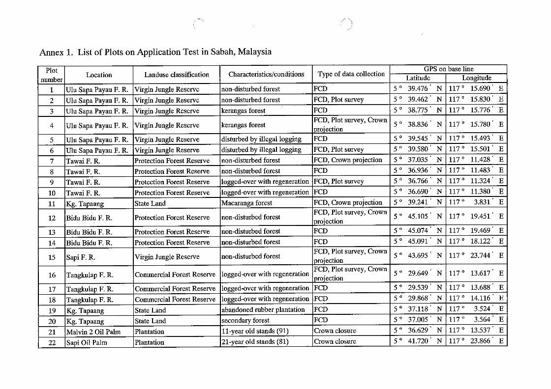
Annex I. List of Plots on Application Testin Sabah, Malaysia

Plot

number

I

2

Ulu Sapa Payau F. R.

Location

3


4


5


6

Ulu Sapa PayauF. R.

7

, \

Ulu SapaPayau F. R.

Landuse classification

8

Virgin Jungle Reserve

Tawai F. R.

9


Tawai F. R.

10


TawaiF. R.

11

Tawai F. R.


12

Kg. Tapaang

VirginJungle Reserve

13

Bidu Bidu F. R.


14

Protection Forest Reserve

Bidu Bidu F. R.

Characteristics/conditions


15

Bidu Bidu F. R.

non-disturbed forest



SapiF. R.

16


kerangas forest

State Land

17

Tanglculap F. R.

kerangas forest

18


Tangkulap F. R.

19

disturbed by megallogging

I\

Tanglrulap F. R.


20

disturbed by illegal logging


Kg. Tapaang

21


Kg. Tapaang

Type of data collection


22


Malvin 2 Oil Palm

FCD

logged-over with regeneration

SapiOilPalm

CoriumercialForest Reserve

FCD, Plotsurvey


CoriumercialForest Reserve

FCD

Macaranga forest

FCD, Plotsurvey, Crownro'ection

ConnnercialForest Reserve


State Land

FCD


State Land

FCD, Plotsurvey


Plantation

FCD, Crownprojection

Plantation


5' 39,476

Latitude

FCD

5' 39,462

GPS on base line

FCD, Plotsurvey


5' 38,775

FCD


FCD, Crown projection

5' 38,836


N

FCD, Plotsurvey, CrownTo'ection

abandoned rubber plantation

5' 39,545

N

1/7' 15,690' ELongitude

5' 39,580

secondary forest

FCD

N

1/7' 15,830

11-year old stands (91)

5' 37,035

FCD

1/7' 15,776

N

21-year old stands (81)

5' 36,936


1/7' 15,780' E

5' 36,766

N


5' 36,690' N

N

1/7' 15,493

5' 39,241

N

1/7' 15,501

E

FCD

N

1/7' 11,428

E

5' 45,105

FCD

N

117' 11,483

FCD

5' 45,074' N

117' 11,324' E

FCD

5' 45,091

E

N

117' 11,380' E

Crown closure

E

5' 43,695

1/7 '

N

Crown closure

E

1/7' 19,451

5' 29,649

E

3,831

N

1/7' 19,469

5' 29,539

117' 18,122' E

5' 29,868

N

E

"

5' 37,118

1/7' 23,744

N

5' 37,005

E

1/7' 13,617' E

5' 36,629

N

E

5' 41,720

N

1170 13,68'

N

117' 14,116

E

N

1/7 '

N

1/7 '

N

1/7' 13,537

E

117' 23.866

E

3,524' E

3,564' E

E

E

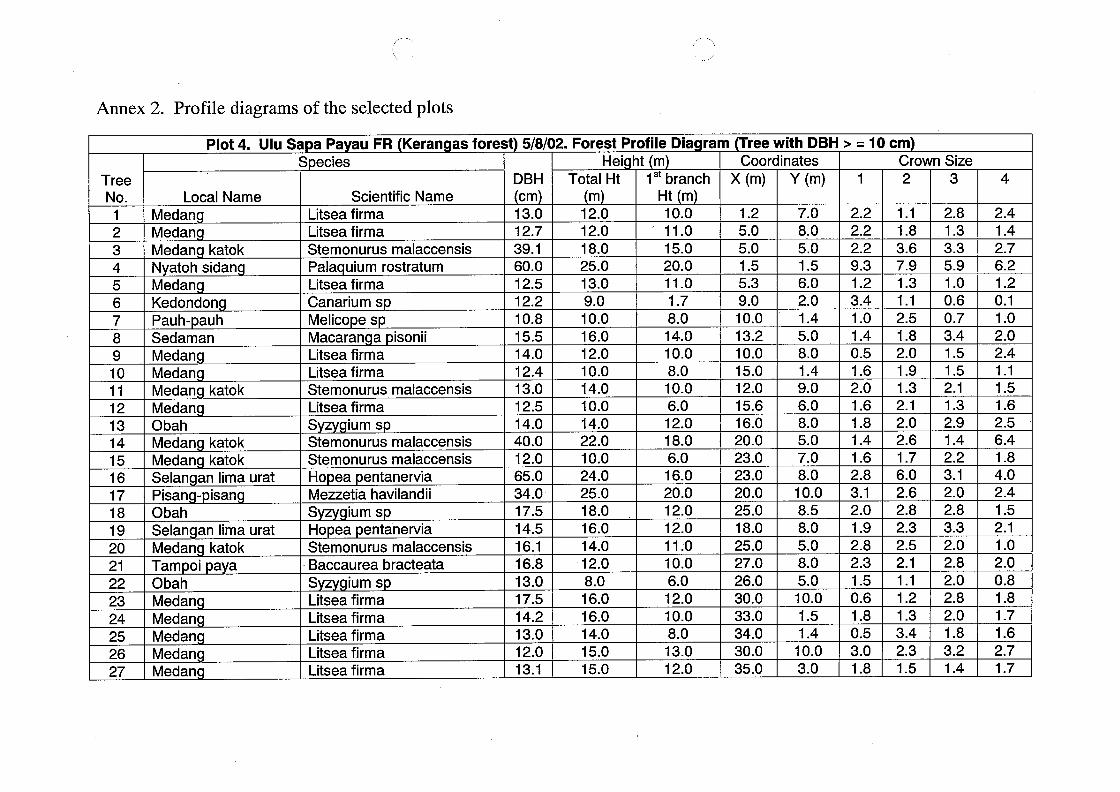
Annex 2. Profile diagrams of the selected plots

TreeNo.

2

Plot 4. Ulu Sa a Pa au FR Keran as forest 5/8/02. Forest Profile Dia

3

Medan

Local Name

4

Medan

5

Medan

6

N atoh sidan

7

Medan

I'I

8

Kedondon

katok

S

9

Pauh- auh

ecies

10

Sedaman

11

Medan

12

Litsea firma

Medan

13

Litsea firma

Medan

Scientific Name

14

Sternonurus malaccensis

Medan

15

Pala uium rostratum

Obah

16

Litsea firma

Medan katok

katok

17

Can arium s

Medan katok

18

MeIico e s

Selan an Iima ural

19

Macaran a isonii

Pisan

20

Litsea firma

Obah

21

Litsea firma

Selan an Iima ural

DBHcm

22


Medan katok

Isan

23

Litsea firma

Tam oi a a

24

13.0

S

Obah

..-\

25

12.7

Total Htin


Medan

39.1

Hei ht

26


Medan

IUm S

60.0

27

Ho

Medan

12.0

12.5

Mezzetia havilandii

Medan

ea entanervia

12.0

12.2

in

Sz

1st branchHt in

Medan

18.0

10.8

Ho ea entanervia

25.0

ram

15.5


IUm S

13.0

14.0

Baccaurea bracteata

10.0

9.0

12.4

ree with DBH > = 10 Gin

Sz

11.0

10.0

Coordinates

13.0

Litsea firma

x (in)

15.0

16.0

12.5

Litsea firma

20.0

IUm S

12.0

14.0

Litsea firma

11.0

10.0

I .2

40.0

Litsea firma

Y (in)

5.0

I .7

14.0

12.0

Litsea firma

8.0

5.0

10.0

65.0

14.0

14.0

I .5

34.0

7.0

10.0

22.0

5.3

17.5

8.0

8.0

9.0

I0.0

14.5

5.0

10.0

10.0

24.0

Crown Size

16.1

2.2

1.5

13.2

6.0

25.0

16.8

2

6.0

2.2

12.0

10.0

18.0

13.0

2.0

2.2

18.0

15.0

16.0

I . I

17.5

9.3

1.4

I2.0

6.0

14.0

I .8

3

14.2

5.0

12

16.0

15.6

3.6

12.0

13.0

3.4

8.0

20.0

2.8

I6.0

7.9

8.0

12.0

I. 4

I .O

20.0

12.0

I .3

4

I .3

16.0

13.1

9.0

1.4

3.3

23.0

12.0

I . I

16.0

6.0

0.5

2.4

5.9

23.0

110

2.5

14.0

8.0

1.6

I .4

20.0

I .O

10.0

I .8

15.0

5.0

2.0

2.7

0.6

25.0

6.0

2.0

15.0

7.0

1.6

6.2

0.7

12.0

18.0

I .9

8.0

I. 8

I .2

3.4

25.0

10.0

1.3

10.0

1.4

0.1

27.0

I .5

8.0

2.1

8.5

I. 6

I .O

26.0

I .5

13.0

2.0

2.8

8.0

2.0

2.1

30.0

12.0

2.6

3.1

5.0

2.4

1.3

33.0

17

8.0

2.0

I . I

2.9

34.0

6.0

5.0

I. 9

1.5

1.4

30.0

2.6

10.0

2.8

I. 6

2.2

35.0

2.8

2.3

1.5

2.5

3.1

2.3

I. 5

1.4

6.4

2.0

2.5

10.0

0.6

1.8

2.8

2.1

3.0

I .8

4.0

3.3

I . I

0.5

2.4

2.0

12

3.0

I .5

2.8

I .3

I .8

2.1

2.0

3.4

I .O

2.8

2.3

2.0

2.0

1.5

0.8

I .8

I .8

3.2

17

I .4

1.6

2.7

1.7

TreeNo.

28

29

30

N atoh sidan

Ulu Sa a Pa au FR Keran as forest 5/8/02. Forest Profile Dia ram

31

Local Name

Obah

32

Slopex-axis

Selan

Medan

Medan

an Iima ural

O-10=-2, 10-20=-I,20-30=-2, 30-40=-I

S ecies

^

Pala uium rostratum

S

Scientific Name

Ho

Litsea firma

IUm S

ea entanervia

Litsea firma40-50=+I

DBHcm

13.7

15.0

Total Htin

I\

Hei ht

30.0

13.5

14.0

14.7

16.0

in

1st branchHt in

19.0

12.0

ree with DBH > = 10 cm

12.0

10.0

11.0

Coordinates

x (in)

7.0

8.0

37.0

6.0

40.0

Y (in)

44.0

47.0

0.9

40.0

6.5

8.0

Crown Size

2.5

14

2

I .O

7.0

I . I

2.0

I .4

1.3

3

0.6

3.3

1.6

3.0

1.8

4

0.4

2.0

I .8

2.5

2.2

0.6

2.2

I .8

I .3

*

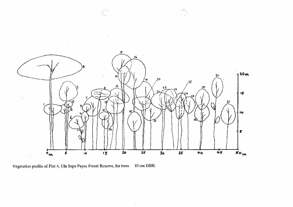
Canopyprofile of Plot 4, Ulu Sapa Payau Forest Reserve, fortrees

C^

I\

GP

a

%

* I6

@

62,

" 23 at

IOCmDBH.

^

@

@

63t

t

,

a, '

"

@

re

*40

a

*a *-, ,, 5.

\

4. -

I+

5

Vegetation profile of Plot 4, Ulu Sapa Payau Forest Reserve, fortrees

11

^* I

,

6

16

,

,

,

,

-\

^.

. " ,

,

,V,

I

I^

13 '~ ~^r. '

10

5

13 2.0

.

10

I,

L

II

13

.

I ,

I,.,

GJ

2.3

,

,

us

,

II

\

\ .

,/

?,

I,,

*. ,,I'

25

I , \

21

2.0

.J

'I'

,

,

2.9

2.9

30

2.5

IOCmDBH.

,

30

^. On

32

31

35

15

^'O

10

4, .5

5'

50r, ,

TreeNo.

2

3

Darah damh

4

Local Name

Kedondon

5

N atoh

6

Peru ok

7

Plot 7. Tawai FR 5/8/02. Forest Profile Dia ram

8

Perah ikan

S ecies

9

N atoh

.^.

10

Ke ala tundan

11

Kedondon

12

M ristica s

N atoh

13

Can arium s

Kedondon

Scientific Name

14

Pala uium rostratum

Min ak berok

15

Lo ho etalum beccarianum

16

Pt

Resak ba'au

17

Elaterios ermum to OS

cho

Kedondon

18

Madhuca s

Malotus sa

19

Buchanania s

Kar us wood

xis kin it

20

Dac odess

Malotus kernen an

21

Madhuca s

Ka u malam

22

DBHcm

Dac odess

Obah

23

ar-sa ar

Xantho h 11um

Selan an batu Iaut

24

57.4

A orusa acuminatissima

Malotus sa ar-sa ar

25

Total Htin

17.5

Vatica inari acha of

26

Hei ht

20.1

Dac odess

Sera a timbau

27

7

10.5

Slope-

Mallotus wra it

Ka ur merah

34.0


13.2

\

H dnocar us woodii

x axis

Kar

16.0

22.5

in

Mallotus enan iana

Ist branchHt in

Ka

24.0

20.6

us wood

Dios

0-10=+23.10-20=+22

14.0

ur merah

63.0

Sz

15.0

22.5

Shorea falciferoides

20.0

18.0

ros s

12.5

Mallotus wra it

I2.0

IUm S

18.0

Coordinates

26.0

A orusa acuminatissima

x (in)

10.0

28.0

27.0

Shorea smithiana

10.0

22.0

14.5

D obalano s becarri

49.4

10.0

17.0

25.8

H

46.1

12.0

Y (in)

13.0

26.0

dnocar us woodii

D obalano s beccarii

46.9

13.0

23.0

12.0

20-25=+6, 25-30=-18, 30-40=-20, 40-50=-21

44.5

22.0

16.0

24.0

I .O

36.5

18.0

25.0

13.5

1.5

35.0

11.0

27.0

I2.5

3.8

33.0

18.0

9.0

Crown Size

22.2

7.6

3.5

35.0

18.0

22.0

39.0

2

I. O

I .O

28.8

12.0

16.0

I'D

2.0

6.0

30.0

18.0

9.5

16.0

12.9

2.6

4.6

18.0

27.0

5.2

23.0

3

85.3

8.8

I .O

26.5

10.0

32.0

5.4

34.7

4.2

I .6

7.3

24.8

16.0

14.0

I .8

20.0

9.0

2.5

2.4

26.0

12.0

4

0.7

14.0

37.0

2.3

7.0

4.8

23.0

11.0

38.0

3.0

7.0

15

3.1

0.4

22.0

19.0

25.0

I .5

9.1

12

2.5

22.0

20.0

I .9

5.0

14.0

4.5

0.9

3.3

3.7

20.8

7.0

24.0

I .9

2.8

4.5

0.9

2.8

13.0

11.0

I .2

4.6

3.9

4.5

5.2

32.0

I2.0

2.0

6.0

3.8

4.0

2.6

20.0

I0.0

2.7

2.4

0.5

2.9

3.0

I2.0

2.5

5.5

3.8

4.5

3.0

2.5

20.0

2.6

4.5

3.0

6.0

3.2

4.2

3.0

3.7

5.0

3.7

I .8

2.2

2.6

5.0

2.4

2.7

I .6

3.4

4.0

0.6

2.4

1.4

3.0

2.0

2.5

I .5

2.0

2.4

2.6

2.9

I . I

I .3

8.3

3.0

1.4

2.7

8.0

1.0

2.9

1.5

3.0

7.0

2.0

0.9

I. 8

1.3

5.0

2.0

1.6

1.9

I .5

1.6

2.7

2.7

7.6

2.4

I. 8

2.8

2.1

2.6

3.5

4.2

7.9

4.2

1.9

3.1

2.2

2.6

7.2

0.9

4.2

4.4

2.6

\

02,

\\

~,,~

%, o3t , .2.01t, z"' ;' '\

,

.

,

,

,

-,

,

25

I~

-L a '~~,-,' ,

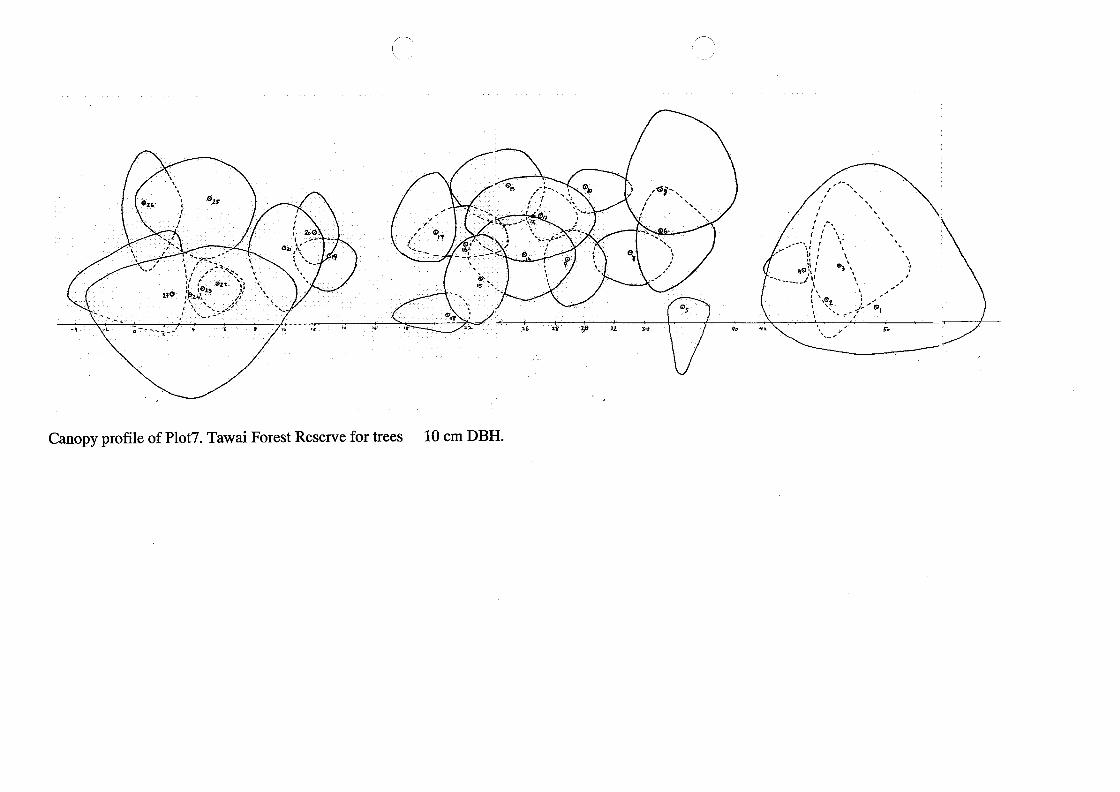
Canopy profile of Plot7. TawaiForest Reserve fortrees

. ** ~~~'*:,,

,

,

*,..,

a@, ,.~

," ,\:e, \

, ~

*,

,

.^

,

,

~.

"

,,,

..

,,

,.

I

^^ ^

q,

,,

. ~.~

@

16, \, .-<

., .,

I~\

.

\

a,,5 ~

'1, I

-.

q,

a

.t

$,

6,

IOCmDBH.

0,

a, ;, 34 e,

03

L@

2.4

a, ^

"2.3

,,.,

16

2.0

14

I,

,

,

,

,

.:, ,..

16

\

Dor

,,-,\\.\\

~~

19

*

19 .\

^

,I,

I I

,,

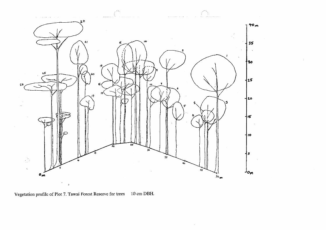
Vegetation profile of Plot 7. Tawai Forest Reserve fortrees

.~~,

,,,

,.--

,,.

,^.

On

I\

3

8

,@

,O

a

,

.

,S

.

*,I

J

20

,

,

6

,1.00^

as

5

35

a.

36

.

I,

30

I ,,..

35

,

IOCmDBH.

2.5

32.0

qo

,5

45

,O

So

5

01.1

TreeNo.

2

3

Lin

Local Name

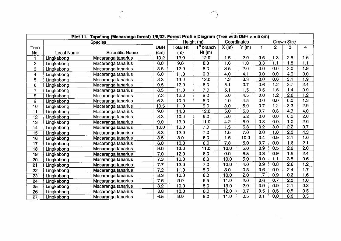
Plot, ,. Ta a'an

4

Lin

kabon

5

Lin

kabon

6

Lin

kabon

7

Lin

kabon

8

Lin

S ecies

I

kabon

9

Lin

\

10

kabon

Lin

11

kabon

Lin

Macaran a forest '18/02. Forest Profile Dia ram

12

kabon

Macaran

Lin

13

kabon

Macaran

Lin

Scientific Name

14

kabon

Macaran

Lin

15

kabon

Macaran

Lin

a tanarius

16

kabon

Macaran

Lin

a tanarius

kabon

17

Macaran

Lin

a tanarius

kabon

18

Macaran

Lin

kabon

19

a tanarius

Macaran

Lin

20

kabon

a tanarius

Macaran

Lin

21

kabon

a tanarius

Macaran

Lin

DBHcm

22

kabon

a tanarius

Macaran

Lin

23

kabon

a tanarius

Macaran

Lin

kabon

10.2

24

a tanarius

Macaran

Lin

25

kabon

a tanarius

Total Htin

6.0

Macaran

Lin

a tanarius

26

kabon

.--\

Hei ht

8.5

Macaran

Lin

27

kabon

a tanarius

\

6.0

Macaran

Lin

13.0

a tanarius

kabon

Macaran

8.3

Lin

a tanarius

9.0

kabon

in

9.5

Macaran

Lin

1st branchHt in

12.0

a tanarius

kabon

8.5

Macaran

11.0

kabon

a tanarius

7.2

Macaran

13.0

a tanarius

reewith DBH > = 5 cm

6.3

Macaran

12.0

12.0

a tanarius

10.5

Macaran

8.0

Coordinates

11.0

a tanarius

9.0

X (in)

Macaran

8.0

12.0

a tanarius

8.3

Macaran

9.0

10.0

a tanarius

9.0

Macaran

12.0

15

11.0

a tanarius

10.0

Macaran

Y (in)

I .6

14.0

8.0

a tanarius

8.3

Macaran

3.5

7.0

10.0

a tanarius

8.5

4.0

13.0

9.0

a tanarius

2.0

6.0

10.0

8.0

4.3

a tanarius

9.0

I .O

9.0

I2.0

5.1

a tanarius

2.0

7.0

12.0

5.1

Crown Size

8.0

0.5

4.1

7.3

9.0

10.0

5.0

2

0.3

3.3

7.7

11.0

4.0

I3.0

0.0

0.7

7.2

7.0

3.0

I .3

12.0

0.0

8.3

I .5

7.0

5.0

10.0

I . I

3

0.0

4.5

7.5

6.0

5.0

0.0

I2.0

0.6

4.5

8.2

2.5

6.0

4.2

0.0

11.0

5.0

0.5

8.8

I .8

11.0

4

1.5

10.0

0.0

5.0

0.0

6.5

2.0

8.0

1.5

I .2

9.0

5.2

0.0

15

4.9

6.0

I. 5

10.0

I .6

6.0

0.7

I . I

3.1

7.8

7.0

10.0

I .2

5.8

0.7

I .9

2.7

10.0

5.0

0.0

9.0

7.0

0.0

0.0

1.4

9.0

8.0

I .2

10.0

0.8

I .9

2.8

10.0

6.5

0.8

5.0

0.2

2.4

0.0

10.0

5.0

0.0

5.0

0.0

0.9

3.3

0.0

8.0

6.0

6.5

0.4

I .2

4.3

10.0

3.0

8.0

5.0

0.7

I .3

0.0

11.0

I. O

0.9

4.0

2.9

I .O

13.0

0.9

0.3

0.5

4.0

2.2

I2.0

0.0

0.0

2.0

2.0

2.0

110

0.5

0.9

2.0

2.0

2.1

0.9

0.6

2.0

0.7

1.6

I . I

0.7

1.7

4.3

2.2

0.8

0.6

0.5

1.0

1.5

0.0

0.9

2.1

3.5

0.9

0.5

2.0

2.6

0.7

0.1

2.4

2.4

0.9

0.6

0.6

0.5

1.2

2.0

0.0

1.7

2.1

1.6

0.5

1.0

0.0

0.3

0.50.5

TreeNo.

28

29

30

Lin

31

Local Name

Lin

kabon

32

Lin

kabon

33

Ta a'an

Lin

34

kabon

Slope

Linkabon

Lin

x-axis

S ecies

.-,~

kabon

Lin

\

kabon

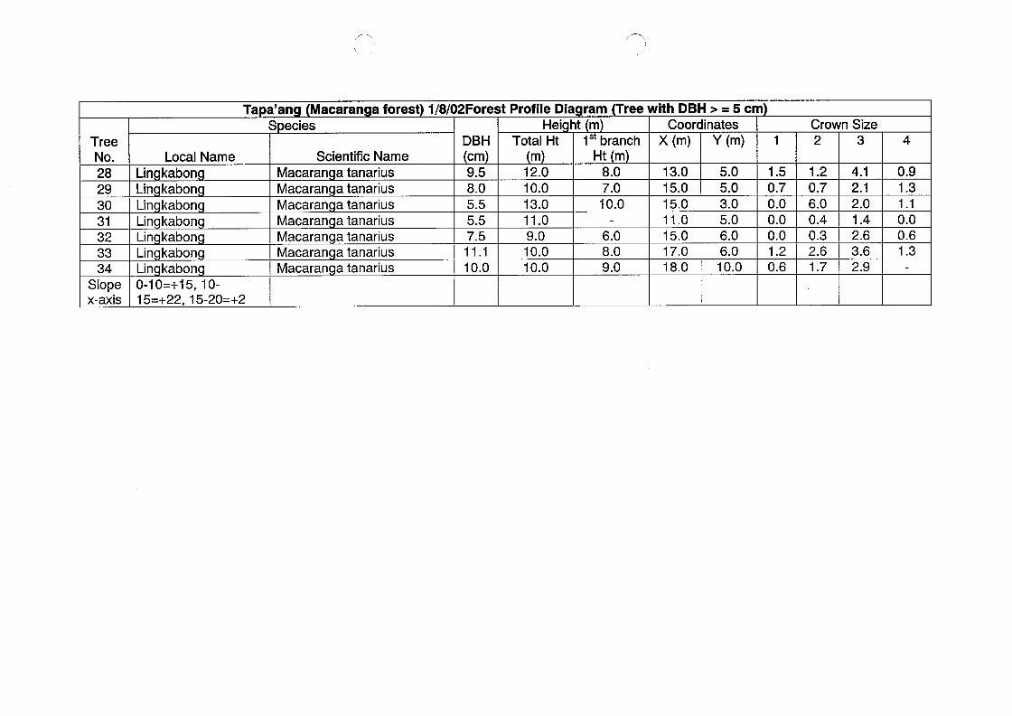
Macaran a forest 1/8/02Forest Profile Dia ram

0-10=+15, 10-15=+22, 15-20=+2

kabon

Macaran

Macaran

Scientific Name

Macaran

Macaran

a tanarius

Macaran

a tanarius

Macaran

a tanarius

Macaran

a tanariusa tanarius

a tanarius

DBHcm

a tanarius

9.5

Total Htin

8.0

Hei ht

,^

5.5

5.5

12.0

7.5

10.0

11.1

in

,st branchHt in

13.0

10.0


11.0

9.0

8.0

10.0

7.0

10.0

Coordinates

x (in)

10.0

13.0

6.0

15.0

Y (in)

8.0

15.0

9.0

11.0

5.0

15.0

5.0

17.0

3.0

18.0

Crown Size

5.0

1.5

2

0.7

6.0

0.0

6.0

I. 2

10.0

0.0

0.7

3

00

6.0

I .2

4.1

0.4

0.6

2.1

4

0.3

2.0

2.6

0.9

1.4

I .7

I .3

2.6

I . I

3.6

0.0

2.9

0.6

I .3

@

15

,.,'^';~.. ~**, " ^,~"~ '~ ,

; 19 ;^", " " ,' ,",,, , 117, ,""., ,, '8"' ^- I I^;, " '""""' '~~"'

~~ A'. .,~~ I~ ..," ,;,,~ I '

*, a. ,\/ . ',,

,@*,. ~";@' I-."<~', ^,;@a. ,,. '^;^a^-,\, ,

;@,,, ,

I~

t

t

,^

,

*

@

Canopy profile of Plot 11. Mac@r@"g" forest at Tapa ang trees

a

61,

,,

,-\

4-

*

6

.

J

,.

.

,

a.

~ -.~-..

632. I, ^ ^

.^... ^

I;^;* ,@Z,

.,

38*

,,

I'

.

,

,,

,,

~^^

a,

--.-

^I^.

03

~-

^ ^ ,

I

~..

^,

JP

13

.,

..

5cmDBH.

,

1.1. 16 ,8 Z@

10

3

^^

I~'

'*'

,,,~J

I'

11

6

I,

22

,

,,

I^

30

26

?.^

,,

24

~~

25'

o

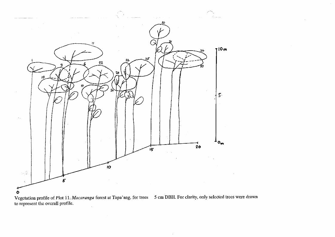
Vegetation profile of Plot 11. M@car@"g" forest at Tapa ang. fortreesto representthe overall profile.

, .\

,\ ,,

~- .>.- --

,,

,

5

,

,

34-

33

10, ,,

10

15

g

20

5 cm DBH. For clarity, only selected trees were drawn

O, ,

TreeNo.

2

3

La an -Ia an

Local Name

4

Sem ilau

5

Resak baau

6

N atoh

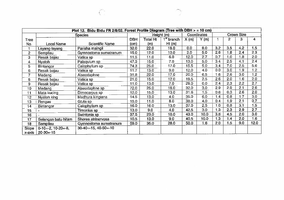
Plot, 2. Bidu Bidu FR 2/8/02. Forest Profile Dia ram

7

Bintan or

8

Resak baau

S ecies

I'

9

Medan

I

10

Resak baau

11

Resak ba

12

Parisha main it

Medan

13

G innostoma sumatranum

Mala kucin

Scientific Name

14

Vatica s

N atoh kin

au

15

Pala uium s

Ren as

16

Calo h

Bintan or

17

Vatica s

18

AISeoda

Slopex-axis

Vatica s

Selan an batu hitam

Urn S

Vatica s

Sem ilau

AISeoda

0-10=-2, 10-20=-8,20-30=-15

hne

DBHcm

Dimocar

Madhura kiri iana

32.0

Gluta s

hne s

Total Htin

15.0

Calo h 11um s

Hei ht

I\

us s

11.5

Timonius s

47.3

Swintonia s

22.0

74.3

Shorea atrinervosa


I2.0

in

11.7

G innostoma sumatranum

1st branchHt in

11.0

31.8

30-40=-15, 40-50=-, O

15.0

21.0

25.0

11.0

18.0

13.0

72.0

10.0

22.0

Coordinates

12.0

x (in)

6.0

15.0

14.5

7.0

13.0

15.0

17.0

0.0

25.0

16.0

Y (in)

9.0

2.0

15.0

13.0

17.0

12.0

13.0

37.5

12.0

13.0

11.0

10.5

8.0

15.5

7.0

16.0

59.0

5.0

12.0

18.0

9.0

2.7

20.0

13.0

23.0

Crown Size

3.2

5.0

19.5

4.0

13.0

2

2.6

5.0

29.0

35.0

8.0

0.7

4.0

32.0

13.0

3.5

3.4

6.5

31.6

4.0

I .8

3

2.5

3.4

35.0

I0.0

I .O

0.0

0.0

4.2

38.0

9.0

2.5

3.0

I .6

2.4

28.0

37.0

4

7.0

2.6

15

42.5

I .8

3.0

2.4

6.0

1.5

4.1

43.0

2.6

4.0

2.9

2.3

40.5

2.5

2.0

2.5

0.6

2.0

50.0

I .9

2.3

3.0

I .4

2.4

3.0

2.9

10.0

0.4

5.6

I .6

0.3

10.0

I .O

I .2

2.2

0.8

1.6

I .3

I .2

2.1

I .9

3.8

2.0

2.6

0.8

I .3

2.7

I .7

2.3

2.0

2.6

2.1

4.5

2.0

3.1

I .4

3.0

2.9

I .5

0.7

2.0

I .5

2.0

2.7

9.0

3.0

1.6

12.0

I~

@

Canopy profile of Plot 12, Bidu Bidu Forest Reserve, fortrees

.

5

I~\

^

8

. co us

IOCmDBH

@

\

@ @

@

S,

".

6 "

,

,, , ",

@

I~'

,

?...

5

4-

3

6

@

^

. I

*^,.,

8

I"

3

Vegetation profile of Plot 12, Bidu Bidu Forest Reserve, fortrees

--\

10

10

q

.

2.0

It

,4-

2.5

16

^. O un

18

30

35

13

I^

IOCmDBH.

35

30

15

2.5

,*@

2.0

^s

,S

3'0

to

5

On

TreeNo.

2

3

Karei utih

Local Name

4

Peru ok

5

6

N atoh

7

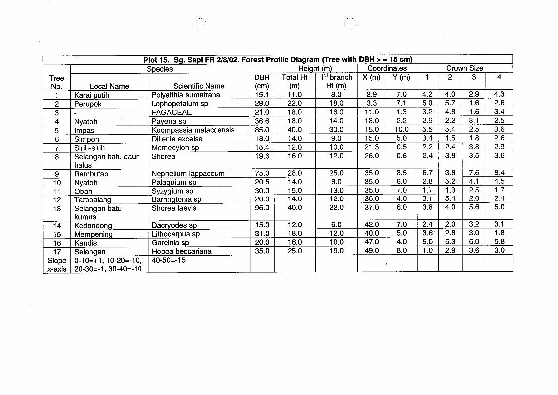
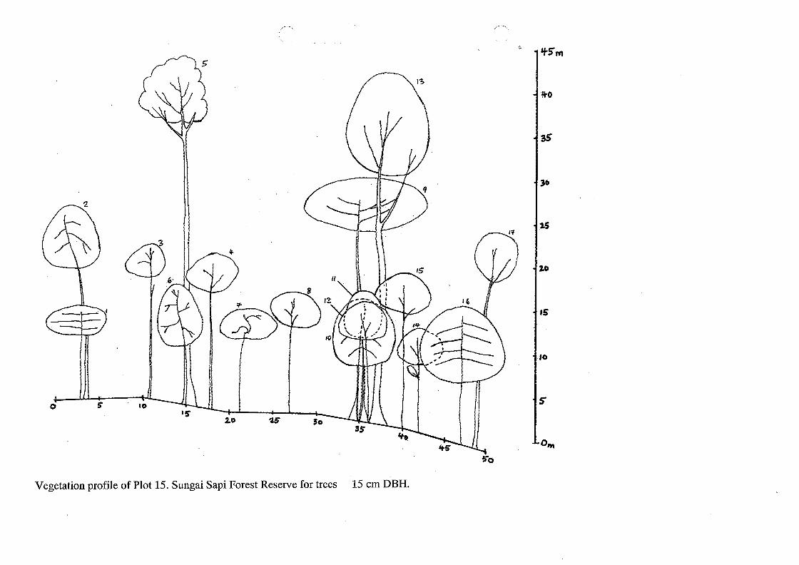
Plot 15. S . Sa i FR 2/8/02. Forest Profile Dia ram

Im as

8

Sim oh

S ecies

I~

Sirih-sirih

9

Selangan batu daunhalus

10

11

Pol

Rainbutan

12

Lo ho etalum s

N

althia sumatrana

Scientific Name

13

FAGACEAE

Obah

atoh

Pa ena s

Tam alan

14

Koom assia malaccensis

Selangan batukumus

15

Dillenia excelsa

16

Memec 10n s

Kedondon

17

Slopex-axis

Shorea

Mein enin

Kandis

Ne helium Ia

Selan an

DBHcm

Pala uium s

0-10=+I, 10-20=-10,20-30=-,, 30-40=-10

Sz

15.1

Barrin toriia s

29.0

Total Htin

Shorea Iaevis

IUm S

21.0

,-\

Hei ht

36.6

aceum

Dac odess

11.0

^

85.0

Lithocar us s


22.0

18.0

in

Garcinia s

1st branchHt in

18.0

15.4

Ho ea beccariana

18.0

19.6

40-50=-, 5

40.0

8.0

14.0

75.0

18.0

12.0

Coordinates

20.5

x (in)

16.0

16.0

30.0

14.0

20.0

30.0

2.9

28.0

96.0

Y (in)

9.0

3.3

14.0

10.0

11.0

15.0

15.0

12.0

18.0

14.0

31.0

7.0

15.0

40.0

20.0

7.1

25.0

15.0

35.0

I .3

21.3

8.0

12.0

Crown Size

4.2

2.2

13.0

26.0

18.0

10.0

2

5.0

12.0

16.0

3.2

5.0

22.0

35.0

25.0

4.0

2.9

0.5

35.0

5.7

3

0.6

5.5

35.0

6.0

4.8

3.4

36.0

12.0

2.9

2.2

8.5

2.2

10.0

37.0

1.6

4

5.4

6.0

2.4

19.0

I .6

I .5

7.0

4.3

42.0

3.1

2.4

4.0

6.7

2.6

40.0

2.5

3.8

6.0

2.8

3.4

47.0

I .8

I .7

2.5

49.0

3.8

3.8

7.0

3.1

3.6

3.5

5.2

5.0

3.8

2.6

I .3

4.0

2.9

7.6

5.4

2.4

8.0

3.6

4.1

4.0

3.6

2.5

5.0

8.4

2.0

2.0

I. O

4.5

5.6

2.8

I .7

5.3

2.4

3.2

2.9

5.0

3.0

5.0

3.1

3.6

I .8

5.8

3.0

I

00

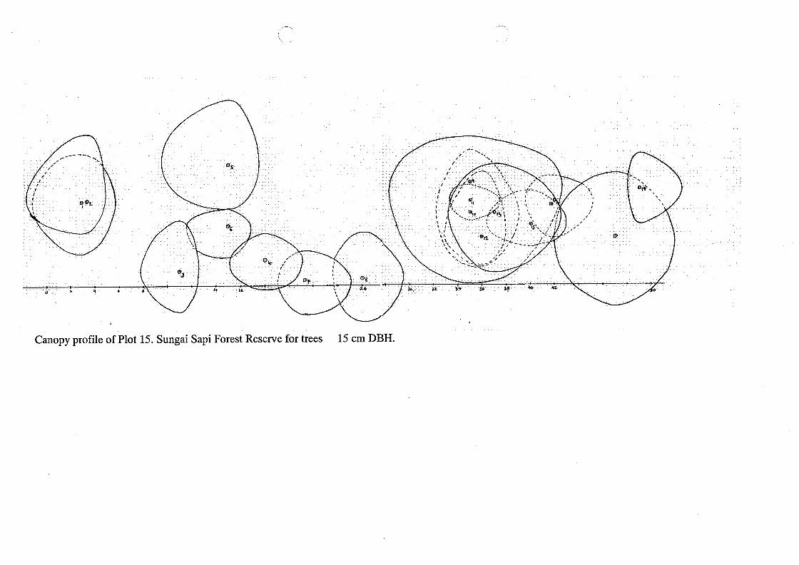
Canopy profile of Plot 15. Sungai SapiForest Reserve fortrees

OS

o

@

I

@

--.\

I.

, , ...-.

I I. ... , 'I , "'.' ,'r",~'.,

' " ,'. 1' 14*

I '... 0, ..../61^, , *'"....' , I , ,'

I '\,' <

\\ , ~~.-.~.

I,

, ~~..

@*

\.

15cmDBH.

30 az ,, a,

\

\\,

,,

38

,,

,,

,

,,

\~

40

~

a'\

43

@

.

\

L

a

5

2

I~\

\

^

^

3

6"

o

4-

13

5

Vegetation profile of Plot 15. Sungai SapiForest Reserve fortrees

.-\

^.

,o

C

11.5m

15

8

11

9

12

4.0

2.0

.

.,

, ,,

. "~

,^^

10

, ,, I

35

15

^. S

,

.

,,

30

go

,,,.

I^

~

16

2.5

~~,

35

,

,

",,

\\

2.0

^..

15cmDBH.

us

"-S

10

5

5'0

O, ,

TreeNo.

2

3

Ka u kerias

Local Name

4

Ka

5

Timbara un

u kerias

6

Obah

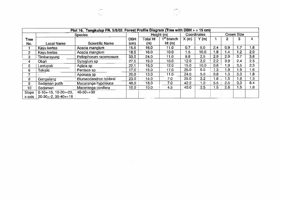
Plot, 6. Tan kula

7

Lantu ak

8

Tekalis

S ecies

I'~

9

10

Slopex-axis

Gan ulanSedaman

Acacia inari ium

Sedaman

Acacia inari ium

O-10=-15, I0-20=-23,20-30=-2, 30-40=+16

Scientific Name

Pelto horum racemosum

FR. 5/8/02. Forest Profile Dia ram

Sz

utih

A

Pentace s

Iaia s

Ium s

A orusa s

Blumeodendron tokbraiMacaran ah o1euca

Macaran a conifera

DBHcm

40-50=+30

15.5

18.5

Total Htin

,-\

33.5

Hei

27.5

ht

16.0

22.1

16.0

reewith DBH > = 15 cm

17.0

in

1st branchHt in

24.0

20.0

19.0

23.0

16.0

48.0

11.0

18.0

15.0

10.0

13.0

Coordinates

x (in)

11.0

14.0

10.0

18.0

12.0

0.7

10.0

17.0

Y (in)

I .5

11.0

6.8

12.0

7.0

5.0

15.0

7.0

10.0

25.0

4.5

2.5

24.0

Crown Size

2.4

3.0

25.0

10.0

2

I .8

42.2

2.9

9.5

40.0

0.9

2.2

5.0

I. 4

3

0.8

3.2

2.9

I .3

I .O

1.7

3.9

0.8

2.5

1.2

4

I .9

I .6

3.7

I .9

5.5

1.6

2.4

I .3

I .5

2.0

3.5

I .5

3.6

I .9

2.5

2.3

5.0

2.6

2.3

I .8

I .6

3.3

I .8

I .5

I .3

6.4

I .8

@

,^\

@

a o

,,

a.

Canopy profile of Plot 16. Tangkulap Forest Reserve fortrees

@

".

I\

e^.

a. + 6

^,.

20

^

23 24 2.6

15cmDBH.

2.8 3 33 39 "

@

39 "o

@

q * %

I,

,.

I\t

,

3

^.

,.

,

,I

I~~

,

I^

,

5

5

Vegetation profile of Plot 16. Tangkulap Forest Reserve fortrees

-\

co

6

...

I:' .e.

OS

>

^,.

2.0

q^

3.5"

15cmDBH.

10

COQ

^o

o0

35

g

00

^S'

50I, ,

On

annex3.

Report on analysis of satellite data for Sabah, Malaysia

I. Analysis of satellite data using the FCD-Mapper ver. 2Newly upgraded methodology that is to be programmed in the FCD-Mapper

ver. 2 was applied to estimate canopy density of the forests surrounding Telupid (Sabah),Malaysia and the results are described below.

1.1 Processing of satellite data for FCD Allaysis in Sabah, MalaysiaLANDSAT ETM data dated May 28, 2002 covering Sabah, Malaysia was

analyzed to estimate the forest canopy density (FCD). Primarily, the single modelthat is programmed in the FCD. Mapper ver. I was applied to process the data forFCD analysis; however, result of the field survey reveals that the FCD valueobtained in this process was relatively underestimated in the mountains where it isexpected to be higher. The underestimation can be attributed to structure of the

forest in the mountains. As Figure 1.1shows, the forest in the mountains consistsof multiple crown layers.

Top LayerA

V

Second Layer

'11. ees constituting the upper layers stand sparsely and are relatively inless amount of leaves; on the other hand, trees constituting the lower layers standdensely between the larger trees and are in more leaves. Although the forest isdense in itself, shadow created by the large trees prevents vegetative

<

Fig 1.1 Forest Condition in Mountain

Shadow

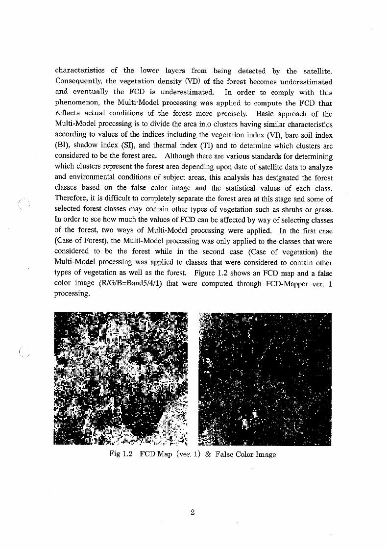
characteristics of the lower layers from being detected by the satellite.Consequently, the vegetation density (VD) of the forest becomes underestimatedand eventually the FCD is underestimated. In order to comply with thisphenomenon, the Multi. Model processing was applied to compute the FCD thatreflects actual conditions of the forest more precisely. Basic approach of theMulti-Model processing is to divide the area into clusters having similar characteristicsaccording to values of the indices including the vegetation index (Vl), bare soilindex(Bl), shadow index (SI), and thermal index (Tl) and to determine which clusters areconsidered to be the forest area. Although there are various standards for determiningwhich clusters represent the forest area depending upon date of satellite data to analyzeand environmental conditions of subject areas, this analysis has designated the forestdasses based on the false color image and the statistical values of each class.Therefore, it is difficult to completely separate the forest area at this stage and some ofselected forest classes may contain other types of vegetation such as shrubs or grass.In order to see how much the values of FCD can be affected by way of selecting classesof the forest, two ways of Multi-Model processing were applied. In the first case(Case of Forest), the Multi-Model processing was only applied to the classes that wereconsidered to be the forest while in the second case (Case of vegetation) theMulti-Model processing was applied to classes that were considered to contain othertypes of vegetation as well as the forest. Figure 1.2 shows an FCD map and a falsecolor image (RIG/B=Bands/4/1) that were computed through FCD-Mapper ver. Iprocessing.

\

; .

Pi',. e

^!

,F1, ' 4.11j. ^*

I*

Fib-f'T

.

..

*^

.,

,

I, ,,;.^

,I

,t

t

I

*^"

, .!^. Q. ,"'..' ' . 'h. *,.,".,.i -^.-.:+^^^*

,,

,

.

I .

.

Fig 1.2 FCDMap (ver. I) & False Colorlmage

'. .r

t .,

It-!;:,;,;,";".,. .

. Jig "..*"., F. ,,

'!;;,;'

a

,

, ,!, I^,,,

2

1.1. I Multi-modelprocessing to compute VD

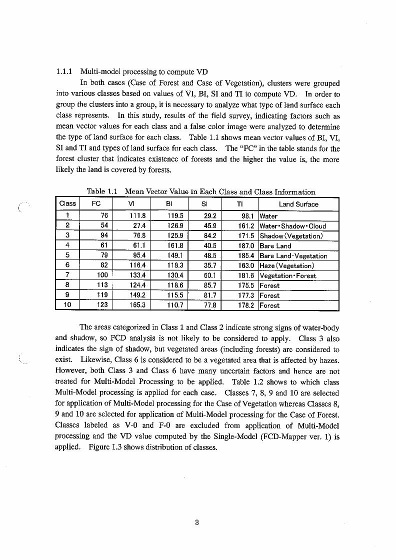
In both cases (Case of Forest and Case of Vegetation), clusters were groupedinto various classes based on values of Vl, Bl, SI and Tlto compute VD. In order togroup the clusters into a group, it is necessary to analyze whattype of land surface eachdass represents. In this study, results of the field survey, indicating factors such asmean vector values for each class and a false color image were analyzed to determinethe type of land surface for each class. Table 1.1 shows mean vector values of Bl, Vl,SI and Tl and types of land surface for each class. The "FC" in the table stands for theforest cluster that indicates existence of forests and the higher the value is, the morelikely the land is covered by forests.

I Class

Table 1.1 Mean Vector Value in Each Class and Class Information

2

FC

3

4

76

5

54

6

Vl

94

7

111.8

61

8

79

27.4

9

82

10

76.8

Bl

100

61.1

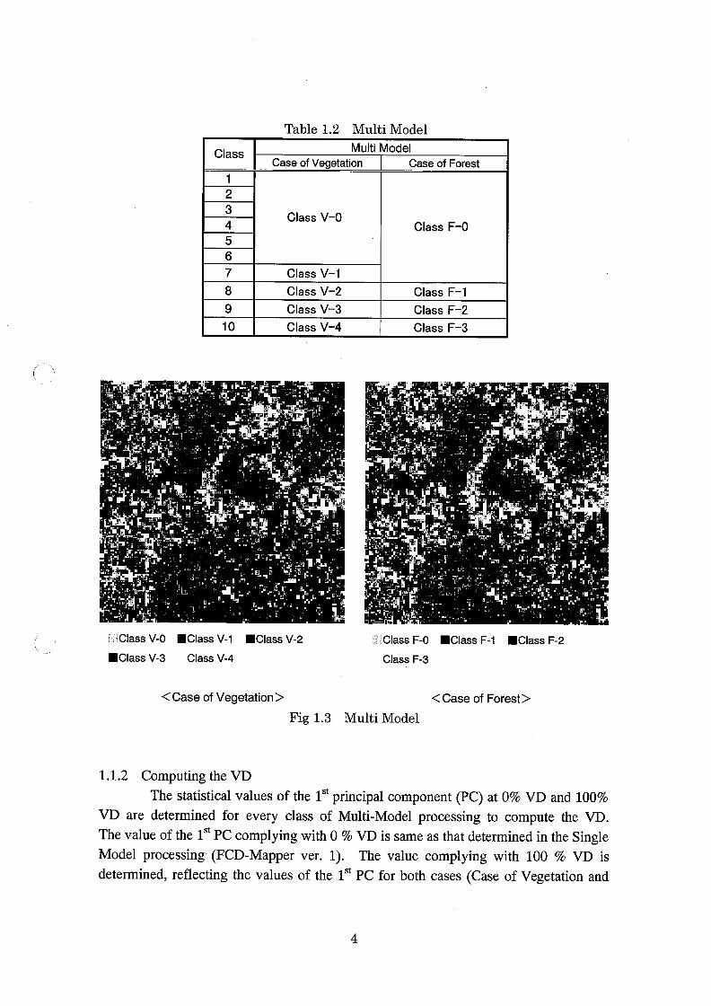
The areas categorized in Class I and Class 2 indicate strong signs of water-bodyand shadow, so FCD analysis is not likely to be considered to apply. Class 3 alsoindicates the sign of shadow, but vegetated areas (induding forests) are considered toexist. Likewise, Class 6 is considered to be a vegetated area that is affected by hazes.However, both Class 3 and Class 6 have many uncertain factors and hence are nottreated for Multi-Model Processing to be applied. Table 1.2 shows to which classMulti-Model processing is applied for each case. Classes 7, 8, 9 and 10 are selectedfor application of Multi-Model processing forthe Case of Vegetation whereas Classes 8,9 and 10 are selected for application of Multi-Model processing for the Case of Forest.Classes labeled as V-O and F-O are exduded from application of Multi-Modelprocessing and the VD value computed by the Single-Model(FCD-Mapper ver. I) isapplied. Figure 1.3 shows distribution of classes.

I I 3

119.5

95.4

11 9

126.9

116.4

123

125.9

133.4

SI

161.8

124.4

29.2

149.1

149.2

45.9

118.3

165.3

84.2

Tl

130.4

40.5

118.6

98.1

48.5

115.5

161.2

35.7

110.7

171.5

Water

60.1

Land Surface

187.0

Water. Shadow. Cloud

85.7

185.4

Shadow(Vegetation)

81.7

163.0

Bare Land

77.8

181.6

Bare Land. Vegetation

175.5

Haze (Vegetation)

177.3

Vegetation. Forest

178.2

Forest

Forest

Forest

3

Class

Table 1.2 MultiModel

2

3

Case of Vegetation

4

5

6

7

Multi Model

Class V-O

8

9

10

Class V-I

Case of Forest

Class V-2

Class V-3

Class V-4

Class F-O

.

.

,

Class F-I

,

Class F-2

Class F-3

ClassV-0 .ClassV-I .ClassV-2

.ClassV-3 ClassV-4

+

*

<Case of Vegetation>

1.1.2 Computing theVD

The statistical values of the I'' principal component (PC) at O% VD and 100%VD are determined for every class of Multi-Model processing to compute the VD.The value of the 1'' PC complying with O % VD is same asthat determined in the SingleModel processing (FCD-Mapper ver. I). The value complying with 100 % VD isdetermined, reflecting the values of the 1st PC for both cases (Case of Vegetation and

^ .

*

^

Fig 1.3 MultiModel

.

'-' ClassF-0 .ClassF-I .ClassF-2

Class F-3

,...,,

<Case of Forest>

4

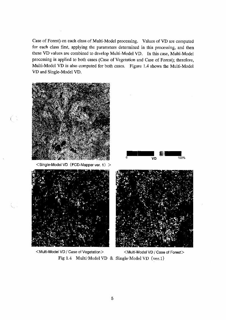
Case of Forest) on each class of Multi-Modelprocessing. Values of VD are computedfor each class first, applying the parameters determined in this processing, and thenthese VD values are combined to develop Multi-ModelVD. In this case, Multi-Model

processing is applied to both cases (Case of Vegetation and Case of Forest); therefore,Multi-Model VD is also computed for both cases. Figure 1.4 shows the Multi-ModelVD and Single-ModelVD.

!^,

I

A\

<4

aI

\

flit-

^^

**

+

a' :.,,.,'

*..*

&:- C

I,

a

<Single-Model VD (FCD-Mapperver. I) >

, ,,' ....*.

. '\:;;.* . 41.4 .. 44*~'.

.

,

A.

..

*

e

,

~.

as * tit, ,o

<Multi-Model VD I Case of Vegetation> < Multi-Model VD I Case of Forest>

Fig 1.4 MultiModelVD & Single. ModelVD (ver. I)

-

VD 100%

.

5

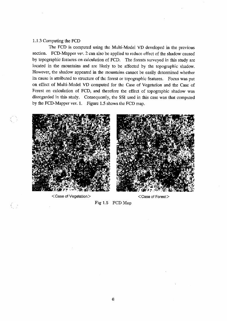
1.1.3 Computing the FCD

The FCD is computed using the Multi-Model VD developed in the previoussection. FCD-Mapper ver. 2 can also be applied to reduce effect of the shadow causedby topographic features on calculation of FCD. The forests surveyed in this study arelocated in the mountains and are likely to be affected by the topographic shadow.However, the shadow appeared in the mountains cannot be easily determined whetherits cause is attributed to structure of the forest or topographic features. Focus was puton effect of Multi-Model VD computed for the Case of Vegetation and the Case ofForest on calculation of FCD, and therefore the effect of topographic shadow wasdisregarded in this study. Consequently, the SSl used in this case was that computedby the FCD-Mapperver. I. Figure 1.5 showsthe FCD map.

,.

*.

f

* ,^

I. .F

,

%1.4 I, +^- ^

e

,i

,

..

I,Q;,;

..

r, "


;,-,

.

F

,

a

a

**

^;!.?

*.I. <

Fig 1.5 FCDMap

, L

%: ^:;,,:!I, , L, .- -

%*

re

- ,.

" I, '

r FFe-

. a* *r,..- 4 '-,'

.

<Case of Forest>

I,

.:.

"

;"

" ..

,on

6

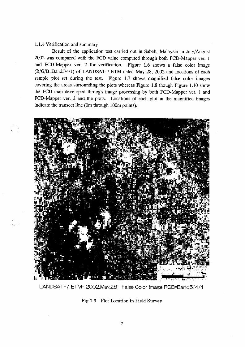
1.1.4 Verification and summary

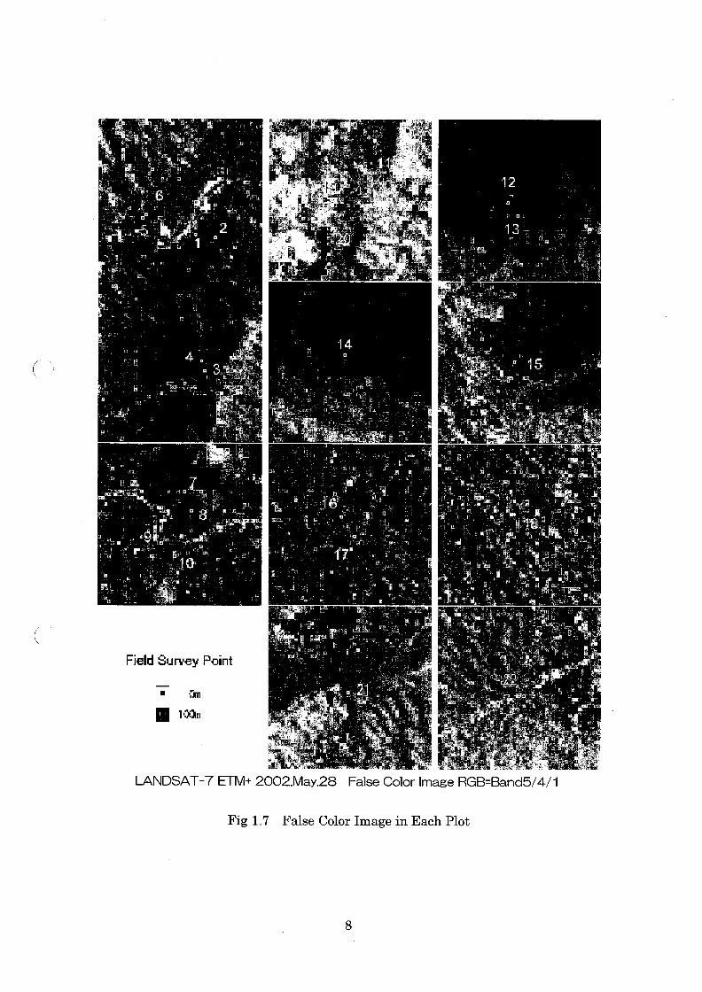
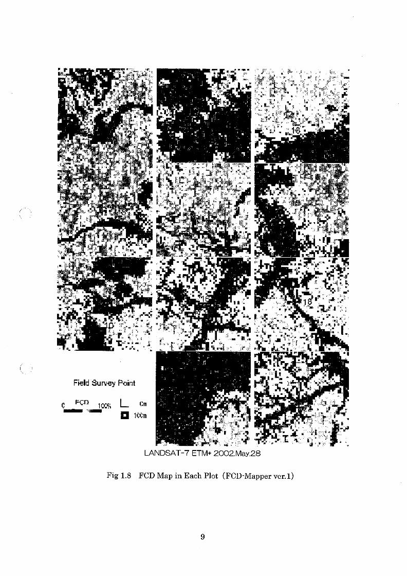
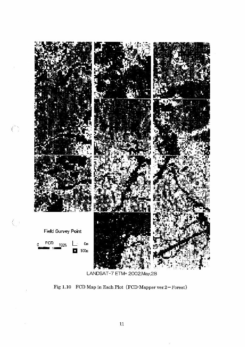
Result of the application test carried out in Sabah, Malaysia in July/August2002 was compared with the FCD value computed through both FCD-Mapper ver. Iand FCD-Mapper ver. 2 for verification. Figure 1.6 shows a false color image(RIG/B=Bands/4/1) of LANDSAT-7 ETM dated May 28, 2002 and locations of eachsample plot set during the test. Figure 1.7 shows magnified false color imagescovering the areas surrounding the plots whereas Figure 1.8 though Figure 1.10 showthe FCD map developed through image processing by both FCD-Mapper ver. I andFCD-Mapper ver. 2 and the plots. Locations of each plotin the magnified imagesindicate the transectline (Om through loom points).

,

,,

,.

,-, f

+,^..,,", ,I^

ipin

,

a"

,.

.

^

,.

. *

"-'- I^ *.;

*",. "

,

^a

a!

a

,r

,*

".

,

*

it .

*

,

.

a

*

LANDSAT-7 ETM+ 2002. May. 28 False Colorlmage RGB. Band5/4/1

Fig 1.6 Plot Location in Field Survey

, "

,

a

a

V

I

,.

*

\

it"

a

.:

^-* , I^.

,.. ,.

;

r

,.

., ^

IF^, ,. :!*' *"' 'ti, ,,

.

.^

7

;I

,,^.:,

!a

.

.

" ,

.!

,

<:1,\,

L .',

,*, j. *.

--;- .

," .

.**;! I ' ' *I'.

*g

. .

,

Field Survey Point

.

. It01/1

:in

LANDSAT-7 ETM+ 2002. May. 28 False Colorlmage RGB=Band5/4/1

. I*

..

^.

,;,

Fig 1.7 False Color Image in Each Plot

.,, I

8

.*,

.,

. ,

*

*

.r

.g.

!.

.., r. I"

" 'a i, ,,.,; ain, *,. , ,,

^';^;^,,' ,..

. .

". .,

J.

I^ -31^;*;

^\.,

"' ' . .;t" ,, ,.,*,.., ill. * :;!'"""""""... . .;,.,.*;"': : ."'\,.-*:"'

" '~"". '1;.;*, I' 'In. 'e, " ,!,'

,* ,., .. "..,* .,*j!.-%,,' . ' ~ .'-;,;.,

I^4'^nit -:^:I' %j'.^.--;11.1^ I*:,,.,, j^,"' ...,,., -. ... ..

It* ,, ,, *^ ^.-;" '""" "~* .,,,. -, 2.54" ' "- ". ".. I:'ul:..,- " " ,.;.

..,

' .' '"~"'. -' 'It,

" ''' """ '' ""' "''4, '""!' ': :*-',*i 13' ,"' ".'---'if, -"*~' ' it "' I*'V'~;',",';',. I, ,. I. .'. + ;.-- it;..@:;,^^,

"..... "

:"--t-,:I, ..- - 11^:-, " *, -.. . ,..,

,

,

ak. "'

,,". .

.,. ,"

,'*, ..

""

I .

\

if

.

D,-*... r {^.... r. 4ii ^I--- .

;j. .* , a- ;

I. :', ...

L!:, a;P"""' '..,.:, .. .

.,.*"!;;,. ,,... . .

."' ^'1<4' ' 11I' ' ' -f, .4-- '~. ~.

.. .,. .^.,..

" ."'\;, '

am"~ ,' *

. ' I. ' .'

. ,..,. . ,.. 11.1

Field Survey Point

L I:inFCDC ICC4^^.^

^ Icem

..,.., .,

,. ",<, i. ..,,"* -.I, .,^- !.;?.,;

'I.

,P^

,

!' ,r

..

,.

,.

,,.

+

^I .'. I

LANDSAT-7 ETM+ 2002. May. 28

Fig 1.8 FCD Map in Each Plot (FCD. Mapper ver. I)

.,.

.,

I-.^. t. ^,.,, , ,....,.!. ': \",'"i ".. .

! r . .\. r. _,.all .,;t . !

: -,,,.....,-..

t^,. P

,., ,

". ;'I^

,.' of, ;

11. . .

,.

.,. ^

r.* ,^ ,I^

^

f. ^, r ^^. t^

ip

^"

."

..

,

.

a:, a;

,

.

,.

: . I

IQ I' ',

.

,,

9

...

I

,.,

$,..

r..

"

,

I,

.

i.

I ;* ':, I' ' """'

, , !*,,*,'

,

P

^.,,

t!

"..

. """ .

'". by.4, '"ri" ,' ".

.

+r ..

^E^;

*.

q

. .~

a. , ^JR. ".',,.*"-!a^\,',', IP'.", ."

* -.

,. ..?. in. , .

* I, .., ,.

'* ,. ,

^

,

P*

.,

,

t

,

.?,

,,

,,'L

Field Survey Point

L CmFCDC ICC4;.^ ^

^ loom

.

..

I.

,rI

,it 431*

", !a, ,-p .+;., jin, **-.'-^',,, ;g. ,,,'- "'4-*,;^;;*,,. I*,, t, ,\,., ..!*.; . I, ;-:^;^..;:

.. ",,..., ,,.".,

' " *-' '",:..!"!"'!$' ' ""' "';* I ', It ,..,-.;; ., L. ,.:

.,,,._,,*,, ,,,. ,..,. ;lit. . '. ' ~in1.1~ 1'4 ,. ,,,! .i, ;.."... ... t

, - I^'11^;in^; " a '-... ,

. ,?^";%,

,

,,*


Fig 1.9 FCD Map in Each Plot (FCD. Mapper ver. 2-Vegetation)

I, I'. .,

,* . ..

,^.'. ',:!..

' I. . ;;! I ~;,'.'^I!I. .. ' .-,'. ~ ^~',!

,;^'::^::'11 I ~,--. ,. -- '1, /1;';.;':"1, '1' , ;,..;;^*._,..,,"' , _ It ..,,. ,,. ", ; , I' ,

*.,, :phip, I-* """".,",. ^..:.,, .:, I. . .,... *,!,.,\*I. *., ,.,,,,^,.: ',,.,.-** -, ,,

... .,

*;'.' *

.

,I,

-;

10

.,. Ir

a

by

,.$

," :..."\--! '~'

I;\

,^I

,,

^,

,*

' 11.1

,

,.

,

,as.r

, -;

*.,

. - : ,. it. *,.L, ,.,.' SE, I';^'*., t -.. . ,~ ".'I

'8;, ,"';!~''

, .. L. "^!

.

.,

., .,,

,

a. .

a

Field Survey Point

L Cm. Icem

FCDC 1, <41.^ ,:^

."

14_.. ,,;\ID ,.,

.r

. .,.

.'I^.

"

.

,

-*-: k:,:, A' I.... ,*

$' ^ i:"" . ,:^L "

!!$;

t^.

$,

.

a,

\,

.I'

J

~,

', a I," ' .,,, ' drip,


Fig 1.10 FCD Map in Each Plot (FCD. Mapper ver. 2-Forest)

"""' '*!?;;;.. er*;., 14 ',%;: I", _..*,, 41i.

; I. ^ *'\ " "" '";,* e'$, *

, ~#

1.1. ,.,

.'. Is '~ '

" !-^:;.!;: ' "" '"", ',, * .:."'

' ., L. ,... ,.

..,'~~. 11. \,$. .,, .' L, ,-,

. .!.. :.,~

.., .., .,.!.,' I, . ; ,$.;;it ',:. i;,.-;';';b, 1:1" ,' . - I, '^", --.;' ,-:1.1!;'-.*:! .,";,;j:"'*'* " I^ t I ,., r, ,,,;.:',"1,111' , "'I, ",.

... ^,,,,..

,

, ~

. b. ,L

11

Comparing the outcomes obtained from analysis by both FCD-Mapper ver. I andFCD-Mapper ver. 2, the FCD values for the latter appear to be higher overall. Inaddition, underestimation of FCD values in the mountain regions caused by analysisthrough FCD-Mapper ver. I was amended upward by applying analysis throughFCD-Mapper ver. 2. Methodology to apply Multi-Model processing to compute VDassured increase of FCD values for both Case of Vegetation and Case of Forest.

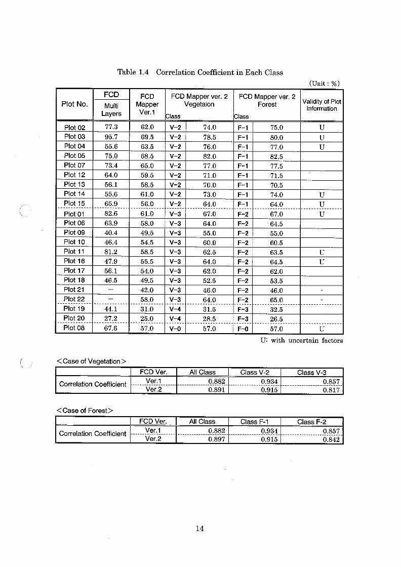
Table 1.3, Figure 1.11 and Figure 1.12 compare the values of crown density for MultiLayers estimated at each plot with the FCD values computed through application ofboth Single-Model processing and Multi-Model processing. In this comparison, theFCD values obtained through Multi-Model processing are also higher than those ofSingle-Model processing. The FCD values for FCD-Mapper ver. 2 score lowercorrelation with the values of ground data as compared to the values for FCD-Mapperver. I overall, but uncertain factors do exist in field information collected at some plots.Values of crown density are not consistent among those who estimate the crown densityat some plots; GPS information collected at some plots is not consistent with theirexpected locations in the satellite image. Such plots should be exduded fromcalculation for verification of accuracy. Comparing these two after excluding theseplots from calculation, correlation of the values for FCD-Mapper ver. 2 becomes higherthan the values for FCD-Mapper ver. I though the difference is not very apparent(Table1.4).

As for comparison between Case of Vegetation and Case of Forest, the FCD valuesscored higher correlation with the ground data in case that application of Multi-Modelprocessing was limited to the forest areas (Case of Forest) as compared to the case thatthe application included other types of vegetation (Case of Vegetation) although thedifference was not obvious. Although application of Multi-Model processing isbasically targeted for the forest areas, the accuracy is not much affected overallif it isapplied to the other types of vegetation,

Every class for the Case of Forest scored increase of the FCD values by applyingMulti-Model processing to compute VD though difference in amount of increasebetween classes exists. However, it is considered that some classes may reflect moreactual condition without application of Multi-Model processing. Provided that the siteconditions are understood to some extent, selecting the classes to apply the Multi-Modelprocessing instead of applying the Multi-Modelprocessing to all classes to compute VDenables us to compute more accurate FCD.

12

Plot No.

Plot 01

Plot 02

Plot 03

TopLa ers

Table 1.3 FCD Values in Each Plots

FCD ( Field Survey)

Plot 04

Plot 05

39.2

Plot 06

23.6

Plot 07

Second

La ers

30.5

Plot 08

43.2

Plot 09

35.8

61.8

Plot 10

57.6

61.5

Plot 11

59.2

Multi

La ers

86.0

Plot 12

37.6

34.6

Plot 13

14.2

56.8

82.6

Plot 14

FCD-Mapperver. I

28.1

31.9

Plot 15

77.3

81.2

24.1

Plot 16

95.7

50.4

47.5

Plot 17

55.6

21.8

26.2

Plot 18

75.0

52.4

61.0

22.8

Plot 19

63.9

FCD-Mapperver. 2

Ve etation

47.5

62.0

Plot 20

73.4

19.0

69.5

51.9

Plot 21

67.6

25.2

63.5

34.8

Plot 22

40.4

10.8

68.5

36.6

46.4

58.0

41.9

67.0

81.2

toriit : %)FCD-Mapper

ver. 2

Forest

65.0

46.4

74.0

64.0

57.0

30.9

78.5

56.1

49.5

37.9

76.0

55.6

54.5

44.1

82.0

65.9

58.5

27.2

64.0

47.9

67.0

59.5

77.0

56.1

75.0

58.5

57.0

46.5

4. *I **F1'.!'!;;;.\*1.1, I!* .

*";1,111!;\;\.!:!!:1111*1:1, :.' '4. ,,.

80.0

61.0

55.0

44.1

77.0

56.0

60.0

27.2

82.5

55.5

62.5

64.5

54.0

71.0

Corr. Coef.

77.5

49.5

70.0

57.0

31.0

73.0

RMS

55.0

25.0

64.0

Top Layers

60.5

42.0

64.0

63.5

58.0

62.0

71.5

+

52.5

70.5

0,774

,I; I' ,-.:;;;'I-';;!1'1'1;.11.1.1:11 *

31.5

e

74.0

28.5

11.8

64.0

46.0

64.5

64.0

62.0

$

53.5

0,700

32.5

Second Layers

Photo

26.5

12.1

46.0

65.0

Top LayerA

->^^,.

Second Layer

0,705

V

,f;;I, ;;.. 11 14:11*inn:;'!.!1, ,,,,,;.;,!"!: .

12.2

$4'

Multi Layers

Shadow

Plot No.

Table 1.4 Correlation Coefficient in Each Class

Plot 02

FCD

Plot 03

Multi

Layers

Plot 04

Plot 05

Plot 07

77.3

FCD

MapperVer. I

\

Plot 12

95.7

Plot 13

55.6

Plot 14

75.0

Plot 15

Plot 01

FCD Mapper ver. 2Vegetaion

62.0

73.4

69.5

64.0

Class

Plot 06

63.5

56.1

Plot 09

68.5

V-2

55.6

Plot 10

65.0

V-2

65.9

82.6

Plot 11

59.5

V-2

Plot 16

58.5

V-2

63.9

74.0

Plot 17

61.0

FCD Mapperver. 2Forest

V-2

40.4

78.5

Plot 18

56.0

61.0

V-2

46.4

76.0

Class

Plot 21

V-2

81.2

82.0

Plot 22

Plot 19

V-2

58.0

47.9

F-I

77.0

V-2

V-3

49.5

56.1

F-I

71.0

Plot 20

Plot 08

54.5

46.5

F-I

70.0

(Unit : %)

58.5

V-3

F-I

73.0

-^

75.0

55.5

V-3

F-I

Validity of PlotInformation

64.0

67.0

80.0

54.0

V-3

44.1

F-I

77.0


49.5

V-3

27.2

67.6

F-I

64.0

82.5

42.0

V-3

F-I

55.0

77.5

58.0

31.0

V-3

F-I

F-2

Correlation Coefficient

60.0

71.5

U

V-3

62.5

70.5

U

25.0

57.0

V-3

F-2

64.0

74.0

U

<Case of Forest>

V-3

V-4

F-2

62.0

64.0

67.0

F-2

52.5

V-4

V-O

F-2

Correlation Coefficient

46.0

64.5

F-2

64.0

31.5

55.0

F-2

FCD Ver.

60.5

U

F-2

28.5

57.0

63.5

U

U

Ver. I

Ver. 2

F-2

64.5

F-2

F-3

62.0

53.5

F-3

F-O

FCD Ver.

46.0

All Class

65.0

32.5

U

Ver. I

Ver. 2

U

26.5

57.0

0,882

0,891

U: with uncertain factors

All Class

Class V-2

0,882

0,897

0,934

0,915

U

Class F-I

Class V-3

0,934

0,915

0,857

0,817

Class F-2

14

0,857

0,842

100%

FCD

90%

80%

,

70%

"~co

. 50%CDor

60%

40%

30%

20%

Fig 1.11

AA

10%

A

^

A

O%

Comparison on the FCD values between results of satellite data analysisand ground survey (Multi. Model; Case of Vegetation)

A

O%

X

10% 20% 30% 40% 50% 60% 70% 80% 90% 100%

Field Survey Data

X

AX-

100%

x : FCD. Mapperver. I

A : FCD. Mapperver. 2

Vegetation

FCD

90%

80%

70%

. : Class V. 2

. : Class V. 3

: Class V. 4

. : Class V. O

us+,coQcoO=

60%

50%

40%

30%

FCD

20%

Fig 1.12 Comparison on the FCD values between results of satellite data analysisand ground survey (Multi. Model; Case of Forest)

oo

o

10%

8<

o

O%

oo

O%

X

10% 20% 30% 40% 50% 60% 70% 80% 90% 100%

Field Survey Data

X

o

x : FCD. Mapper ver. I

O : FCD. Mapper ver. 2

Forest

. : Class F. I

. : Class F. 2

: Class F. 3

. : Class F. O

FCD

15

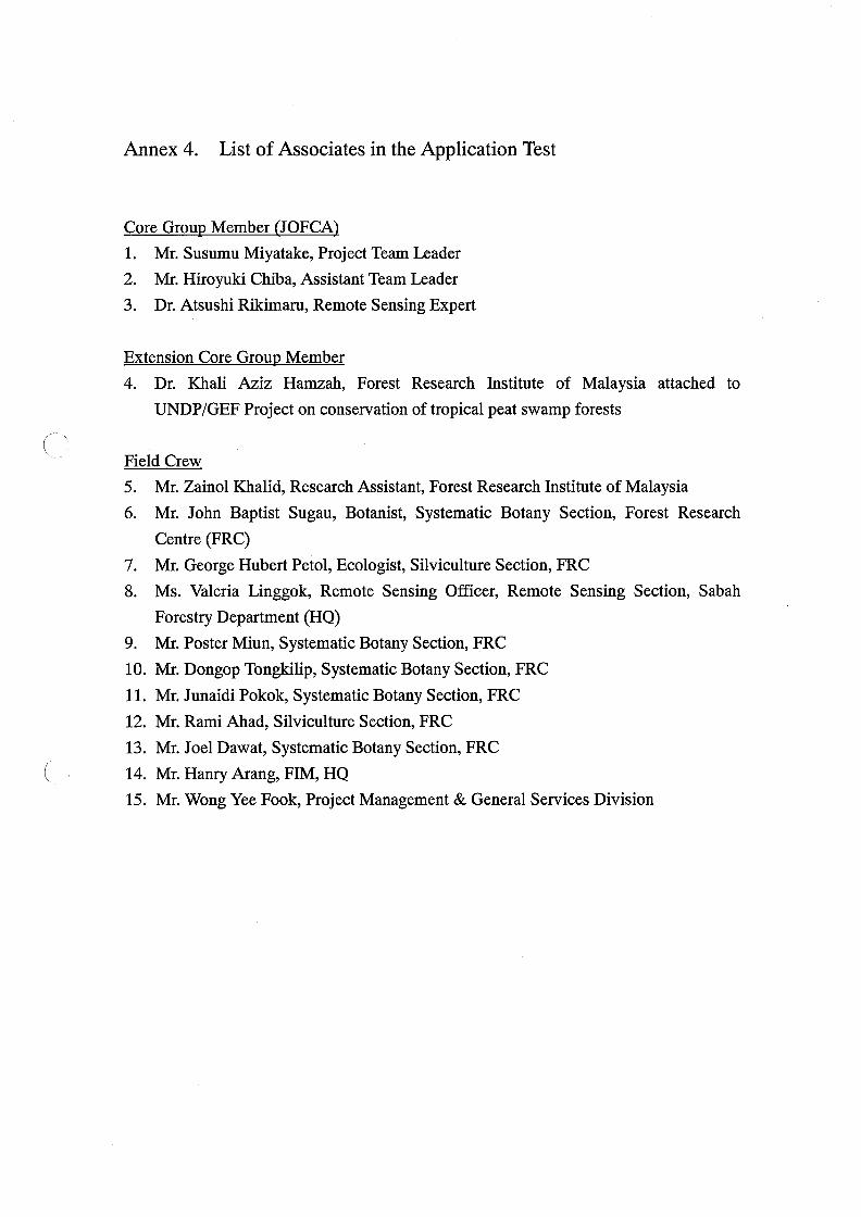
Annex 4.

CoreGrou Member

List of Associates in the Application Test

I. Mr. Susumu Miyatake, ProjectTeam Leader

2. Mr. HiroyukiChiba, Assistant Team Leader

3. Dr. AtsushiRikimaru, Remote Sensing Expert

Extension Core Grou Member

\

4. Dr. Khali Aziz Hamzah, Forest Research Institute of Malaysia attached to

UNDP/GEF Project on conservation of tropical peatswamp forests

10FCA

Field Crew

5. Mr. Zainol Khand, Research Assistant, Forest Research Institute of Malaysia

6. Mr. John Baptist Sugau, Botanist, Systematic Botany Section, Forest Research

Centre (FRO

7. Mr. George Hubert Petol, ECologist, Silviculture Section, FRC

8. Ms. Valeria Linggok, Remote Sensing Officer, Remote Sensing Section, Sabah

Forestry Department(HQ)

9. Mr. Poster Miun, Systematic Botany Section, FRC

10. Mr. Dongop Tongkilip, Systematic Botany Section, FRC

11. Mr. Iunaidi Pokok, Systematic Botany Section, FRC12. Mr. RainiAliad, Silviculture Section, FRC

13. Mr. 1061 Dawat, Systematic Botany Section, FRC

14. Mr. Hanry Arang, F1M, HQ

15. Mr. Wong Yee Fook, Project Management & Generalservices Division

\

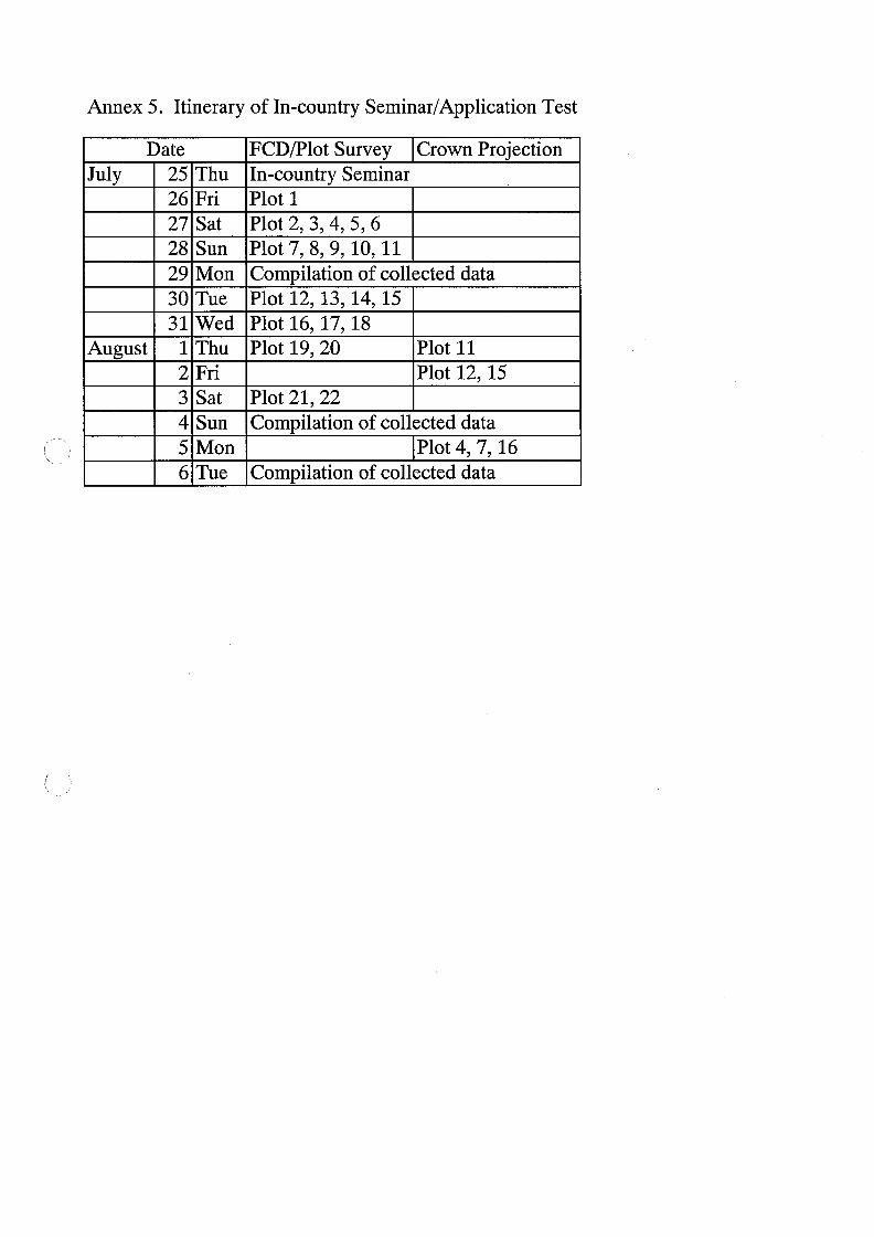
annex 5. Itinerary of In-country Seminar/Application Test

July

Date

25 Thu

26 Fri

27

FCD/Plot Survey

Sat

28

In-country Seminar

August

Sun

29

Plot I

Mon

30

Plot 2, 3, 4, 5, 6

TUG

31

Plot 7, 8, 9, 10, 11

\

Wed

Compilation of coll

I Thu

Plot 12, 13, 14, 15

2 Fri

Crown Projection

Plot 16, 17, 18

3 Sat

Plot 19, 20

4 Sun

5 Mon

Plot 21, 22

6 TUG

Compilation of coll

cted data

Compilation of collected data

Plot 11

Plot 12, 15

cted data

\

Plot 4, 7, 16

i~' (f) itto project fd 60199 rev. fcd modelto monitor ......floor vegetation was recorded to...

Documents