i tiib young person's guide to the data a survey lecture

•

I •

I -

©

Oi on

TIIB YOUNG PERSON'S GUIDE TO THE DATA

a survey lecture prepared for the 196R AF08R-IPP-8t«ntord Conference

Computation of Turbulent Boundary Layers L ^ /

<

Donald Coles Professor of Aeronautics. California Institute uf Technolcxiy

Consultant, The iRAND Corporation*

I. INTRODUCTION

The business of this conference Is to judge the present and potential value of various methods for calculating the development of the turbulent boundary layer in a pressure gradient. My task in this introductory lecture is to classify and criticize the available data, so that any comparison of measured and predicted quantities can include some estimate as to the quality and completeness of the various experiments. It goes without saying that I will try to do this without prejudicing any of the antilytical ideas which may be considered by other speakers at this conference.

I have already dealt with the special case of flow at constant pressure, in an unpublished appendix to Rand Report R-403-PR (Coles 1962). My principal conclusions in that paper weret

(1) that a detailed classification can readily be carried out using the conventional similarity laws, although not much can be learned about the numerical value of the supposedly universal constants;

(2) that there apparently does exist a standard or normal configuration for the flow in question, at least when viewed in terms of the mean-velocity profile alone; and

(3) that among the factors which can adversely affect the quality of a standard boundary-layer flow, the most important are (a) three-dimensional effects and (b) poor judgment in the choice of tripping or thickening devices.

In the present survey, I will again sort through a large mass of data in an effort to detect patterns and conventions which aid in classification. It turns out that a weight has to be assigned to each experiment almost from the beginning, and that this weight is not necessarily the same when considering matters of technique as it is when choosing test cases for calculation or for publica- tion in the proceedings of this symposium. From one point of view, those data turn out to be most useful in which only one factor is varied at a time. If the external conditions change, the instrumentation should remain the same, and conversely. From another point of view, there appears to be a certain level above which measurements can be described as being of professional quality. Such measurements are not only marked by good technique, but are usually also aimed at some particularly interesting or difficult area of the boundary-layer problem rather than at areas which have

* Any views expressed in this paper are those of the author. They should not be interpreted as reflecting the views of the RAND Cor- poration or the official opinion or policy of any of its govern- mental and private research sponsors.

Reproduced by the CLEARINGHOUSE

for Federal Scientific & Technical Information Springfield Va 2?151

..... uufc'bemi appiu'^ .iecse an<d »ale; it?

i-.r.limi*«^

ör 0CT20!9bti

J^

been adequately explored in the past.

One obviouii and venerable example is the contribution by I-udwicq and Tillmann (1949), who studied the effect of both positive and negative pressure gradients using the same impact-probe rake and heated-element instrumentation. Constructive work has also been done by Klebanoff and Diehl (1951) on the effect of initial conditions in flow at constant pressure, and by Bradshaw (1967) on the effect of initial conditions in a diffuser flow. I have several other favorite experiments; for instance, I will draw some delicate conclusions in section III, with the aid of some mea- surenents by Schubauer and Klebanoff (1950) and by Bauer (1951), respectively, about possible effects of streamwise wall curvature and of probe size on apparent profile shape. In most cases these conclusions were not at issue in the original research, and the fact that they can be drawn at all is almost a definition of the professional experimental touch.

Circumstances have required certain measurements to be omitted, deliberately or otherwise. For almost all of the experiments discussed here, tabulated mean-velocity profiles and other data are avoilüble in the literature or have been supplied by the experimenters. In two cases, however, the data have been read from small figures in the original report, and their accuracy should be dis- counted accordingly. The first such case is the thesis by Gruschwitz (1931); the second is an NACA study of an airfoil boundary layer and wake by Mendelsohn (1947). Apparently it has been a practice at NACA to destroy raw data records after a lapse of a few years. Inasmuch as most of the NACA airfoil research of this period involved small models at relatively low Reynolds numbers, I doubt that the effort required to recover the data is worth while in general.

I should also mention several diffuser studies for which data have been provided by the authors, but which I have been forced to set aside, at least temporarily, because of lack of time. These data are potentially useful in support of the main body of material considered by this symposium. However, in my opinion they are not likely to lie near the center of attention, which I expect to be the problem of relaxation phenomena. In this class are the diffuser experiments by Sandborn and Slogar (1955), by Furuya (1958), by Sandborn (1959), by Rosenberg and Uram (I960), and by Spangenberg et al. (1967) . J have also chosen for the present to omit data on reattaching flows obtained by Mueller (1961) and by Plate and Lin (1965), although measurements of this kind will undoubtedly play an important role in future research.

A number of measurements in axially-symmetric geometries are included in the test series but are not included in this survey. The reason is that I do not yet know how to handle an axially-symmetric coordinate system when the tests to be applied to the data are as systematic and delicate as the situation seems to allow — and in fact to require — in the case of plane flow.

Finally, I am compelled to comment on what I consider to be a general failure to exploit the advantages of hot-wire anemometers for measurement of mean as well as fluctuating quantities. As a consequence of this failure, all of the experiments considered in this survey include an unknown influence of the local turbu-

'

Mi

r

\ lence field on measurements of mean velocity by means of total- head tubes.* I suppose that data free of such effects will eventually become available in quantity, but this is not likely to happen soon. On the whole, therefore, I think that it is prefer- able at present to accept these effects as part of the data, rather than to attempt to remove them by unreliable or at any rate un- proven methods.

II. SIMILARITY LAWS

In any survey of this kind, it is important to use the light- est analytical skeleton which will bear the weight of the data. For this and other reasons, I have again chosen to work with similarity laws, although I have little doubt that the same general conclusions could also be reached by other means.

My analysis begins with the idea that a typical boundary- layer flow can be viewed as a wake-like structure which is con- strained by a wall. The wake-like behavior is apparent in the phenomena of intermittency and entrainment and in the sensitivity of the outer profile to pressure gradient. The wall constraint is felt mainly in the viscous sublayer and in the logarithmic part of the profile, and is closely related to the magnitude >f the surface shearing stress.

The idea that there are two distinct scales in a turbulent boundary-layer flow is an old one, although quantitative expressions of this idea have evolved very slowly. A schematic representation of a typical profile is shown in the sketch. To the

*T *■

WALL COMPONENT

WAKE COMPONENT

COMPOSITE PROFILE

'

extent that the outer velocity boundary condition for the inner (wall) profile is the same as the inner velocity boundary condition for the outer (wake) profile, the turbulent boundary layer

* Newman (1951) made a partial correction for turbulence; both the corrected and uncorrected data have been obtained and are considered in this survey.

ff

is a singular perturbation problem of classical type. In fact, we can claim to have discovered empirically the first two terms in a composite expansion, complete with logarithmic behavior. A corresponding physical view is that appreciable transfer of energy to the turbulent motion occurs at the largest scale, and that this energy is eventually converted to heat at the smallest scale (the sublayer thickness). Both of these notions become less opaque as the Reynolds number becomes very large, and it is possible to per- ceive dimly an analogy between the Kolmogorov inertial range and the logarithmic profile, both being manifestations of equilibrium at intermediate scales. It is also reasonable to think of the process of enercy transfer as having a natural direction, and to expect a peculiar behavior when the initial energy distribution is highly abnormal.

The two similarity laws to be cited here are known as the law of the wall and the law of the wake. The most important property of the law of the wall is that it provides a quite plausible method for estimating surface friction.* The essence of this similarity law is perhaps best recognized from its use in describing the profile of the natural wind, for which neither an overall thickness nor an origin for the coordinate system can be defined. I am not aware of any convincing theoretical derivation of the law of the wall; i.e., one which does not at some stage fall back on dimensional analysis in order to adduce a viscous characteristic scale in a region of complete turbulence. Much of the empirical evidence in favor of the law comes from measurements in pipes, and in fact the commonly accepted value of Karman's constant is directly traceable to Nikuradse's pipe experiments. More recently, a thorough calibration of the device called a Preston tube has been carried out by Patel (1965) in pipe flow.** His results are shown as the lowest curve in figure 1. The coordinates are the usual ones for the law of the wall, with u the velocity corresponding to the observed dynamic pressure, and y the distance from the probe center to the wall (i.e., half the probe diameter). If the law of the wall is generally valid, these data should define the position of the first data point in any profile measured with a cylindrical probe.

The most important property of the law of the wake is that

* For historical purposes, it is worth noting that Ludwieg and Tillmann (1949) did not set out to show the general validity of the law of the wall, but stumbled on this result while investi- gating momentum-balance anomalies arising from use of the momentum- integral equation near separation. A careful reading of their de- scription of the calibration of their heated element is also in- structive, since this calibration was (to say the least) somewhat indirect. ** The major problems in such a calibration, given an undisturbed flow of high quality, are (a) to determine the static pressure which would exist in the absence of the probe, and (b) to minimize any non-local disturbances to the mean flow when the probe is present. These problems seem to have received careful attention in Patel's work.

it avotdi a dlfct confrontation with th« phyical mechaniam of ahaar turbulence" In order to uae thia law, It is not necessary to darlv« or even to explain the profile in a wake, but only to know what it looks like — and also to believe that the same processes play a role in boundary-layer flow. In this sense, the concept was apparently first proposed by lludimoto (1935). Hudimoto used a power law rather than a logarithmic law to isolate the part of the mean profile not directly affected by the wall, and he referred to the resulting function as jet-like rather than wake-like, but the spirit is essentially the same as the spirit of my own paper published 21 years later. Hudimoto wrote in English; so much for the hazards of publishing in an unreceptive atmosphere.

The similarity laws are explicitly displayed in my standard equation for the mean-velocity profile (Coles 1956),

5-- f^) ^w (*). (1)

where u-r2 ■ TW/O . The function f (the law of the wall) has the form

yu | yu

outside the sublayer, which is to say for yur/v > 50. The constants K and C are taken as 0.41 and 5.0 respectively, indepen- dent of pressure gradient. For analytical convenience I have represented the function w (the law of the wake) as

w(^) - 2 sin2 (J^). (3)

On putting U ■ Um and y » 5 in the profile formula (1), the local friction law is obtained in the standard form

ö« 1 fiUT 2n — = i in (—-) + C + •=■" . (4)

Given K, C, V, and Ü , the last equation evidently determines any one of the three parameters uT, t, 2 if the other two are known. Since equation (1) defines a two-parameter family of mean-velocity profiles, I have chosen to attack the data bv finding values of two parameters I and uT for each profile such that the rms deviation of the data from the formula (1) is minimized (data points for which yurA < 50 or y/E. >1 are of course excluded). This procedure was originally developed in an attempt to salvage some data for which some or all of the mean-velocity profiles were incomplete (e.g., Riabouchinsky (1914), Perry (1966)). It was next applied, mostly out of a sense of pique, to several flow situations for which the profile formula (1) has been set aside by the authors or others as possibly inappropriate (e.g.. Perry (1966), Stratford

• (1959)). Inasmuch as the procedure turned out to provide a very stable and well-controlled vehicle for classification, it was ultimately applied to the whole of the data.

It became apparent early in this process that the fitting region would have to be more carefully specified. One reason is that the formula (1) has an abrupt change in slope at the outer

edge of the layer, where d(Ü/uT)/d(y/5) changes from I/K to 0. This is an obvious deficiency, and I will come back to it in section IV. At this stage of the development, it suffices to take the experimental existence of the corner into account by limiting the fitting region to the range y/6 < 0.9 or less, partly to avoid unnecessary dispersion and partly to restrict the use of the formula to regions where it has some prospect of being accurate. The phrase "or less" means that the value 0.9 is satisfactory when the wake component is large, but has to be decreased to about 0.75 for flow at constant pressure, and to something like 0.6 as the wake component vanishes.

Moreover, I found in some but not all cases a significant disagreement between the data and formula (1) in the 10 to 15 percent of the profile nearest the wall, as illustrated for several flows in figure 1. On the assumption that this discrepancy could eventually be rationalized as experimental error, the lower limit of the fitting region was adjusted to exclude the data in question. I want to emphasize, however, that the upper and lower limits for fitting were not chosen capriciously for each profile, but were fixed for all the profiles of any one flow (except in the special case of flows undergoing relaxation, and occasionally also for data at very low Reynolds numbers).

The profile parameters obtained from this process include Cf, n, and 6, all determined in a self-consistent way. Note that C, is now being determined by a fit of the central part of the complete profile to the full formula (1), rather than by a fit of the inner profile alone to the law of the wall (cf the remarks in the "Memorandum on Data Selection" which follows this survey paper). The main effect of the change is usually to reduce C, by perhaps one or two percent. Note also that the parameters H and 6 are now differently and more realistically defined than was the case in my 1956 paper,since the existence of a discontinuity in slope at y = & is now being taken into account.

To sum up: points near the edge of the boundary layer have been omitted from the fitting operation on the ground that the data are correct but the formula is wrong, and points near the wall have been omitted on the tentative ground that the formula is correct but the data are wrong, due (say) to effects of wall interference and/or effects of local strong turbulence. For the majority of the flows studied, this procedure seems to be entirely adequate. The fit is usually good enough so that the results are quite insensitive to minor changes in the size of the fitting region. In fact, a typical rms scatter of the data about the fitted curve in the fitted region is two or three parts in 1000 (referred to free- stream velocity). This conclusion may come as a pleasant surprise to some experimenters; it also provides a challenge for theoreti- cians who work independently of the profile formula (1). After

i1 careful study, I have not found any consistent pattern in the re- [ maining small discrepancies, and so I cannot suggest a better ana-

lytical representation for either of the functions f or w than"" the simple functions used here.

? . THE VARIOUS PROFILK PARAMETERS AS DETERMINED BY THE METHODS JUST DESCRIBED ARE LISTED IN TABLE I AT THE END OF THIS PAPER.

■Hai

Finally, I have reexamined the problem of evaluating inte- f. gral thicknesses for profiles which are defined by relatively few

data points near the wall, especially when the Reynolds number is also small. The problem is illustrated in figure 2, which shows the ratio H32 = 63/6 (energy/momentum) plotted against the ratio Hi2 = 6*/6 (displacement/momentum). The upper curve, labelled (a), snows values taken directly from the standard tables supplied to the predictors, together with some additional data points obtained by the same methods. I did not expect that the data would define a single curve, because there must be a Reynolds-number dependence in such a presentation; but in fact the scatter turns out to be wholly unacceptable. Matters are improved in the middle curve (b), which is the same as (a) except that I have deleted all data for profiles which lack experimental definition for U/O less than 1/2. As might be expected, the offending data points correspond to some or all of the profiles in flows 1400, 1800, 3100, 6100, and 6200, among others. These data cover a wide range of Reynolds numbers, and the difficulty must therefore arise in our original choice of an unrealistic interpolation method for the numerical integration near the wall, in any event, it is clear that very little use can be made of these particular data until some better interpola-

| tion scheme is specified. ■

For the sake of consistency, therefore, the integral thicknesses have been recalculated for all of the flows listed in Table I after replacing the experimental data near the wall by standard-

functions, with the results shown in curve (c) of figure 2. The standard sublayer profile is a slight revision of one which 1 have used before, and takes into account recent measurements by Liu (1966), Bakewell (1966), and others. All that needs to be known about the standard sublayer profile in order to reproduce the tabulated thicknesses is that

50 J (U/uT)d(yuT/v) = 540.6;

0' T T

50 , f (U/uTrd(yu /v) = 6546;

50- 3 f (U/u ) cl(yu /v) = 82770.

O1' T T

The gap between yu./v = 50 and the first point used in fitting is filled in by formula (1) with the (sin)^ function replaced by one term in y^, and the integration is then continued numerically by the usual parabolic interpolation scheme. I consider the revised values of displacement, momentum, and energy thickness to be sub- stantially more credible than the original ones, inasmuch as interpolation between measured points near the wall is now on a sounder

0 basis.

THE INTEGRAL THICKNESSES AND RELATED QUANTITIES DETERMINED BY THE METHODS JUST DESCRIBED ARE ALSO LISTED IN TABLE I AT THE

i * END OF THIS PAPER. 1

I

I

III. FLOWS IN OR NEAR EQUILIBRIUM

In this section I will consider only flows for which the profile formula of section II definitely provides a good representation of the data. This class seems to include nearly all equilibrium or near-equilibrium flows and nearly all flows of airfoil or diffuser type. I have not always limited myself to data which are being officially considered at this conference, and in some cases I have changed the emphasis slightly.

Figures 3 and 4 show the result of the fitting operation for several flows which are close to equilibrium in the sense of Clauser's definition. What is plotted is the wake component alone. That is, the fitting operation described in section II has first been carried out for the central 50 to 80 percent of the profile, and the logarithmic part has then been subtracted out.

In almost all cases, there are difficulties in the region close to the wall, even though points for which yuT/v is less than 50 are omitted. These difficulties may well be an instrumentation problem; they will be discussed in more detail at the end of this section, when more data have been put in evidence. The seeming in- crease in scatter in figure 4 as the pressure gradient becomes more negative is due to the fact that a smaller fraction of the velocity profile — in the worst case, as little as five percent — is being displayed in the figures. That the notion of a wake component still makes sense under these conditions is a compliment both to the skill of the experimenters and to the quality of the similarity laws.

There are also systematic discrepancies, especially in figure 4, near the outer edge of the layer; this is the corner effect mentioned in section II. In order to look at this effect more closely, I have converted the data of figure 4 into residuals, or differences between the data and the profile formula, with the result shown in figure 5. The ordinate is AÜ made dimensionless with uT, on the assumption that the corner effect is associated most closely with the law of_the wall. The maximum error in velocity is about one percent of Uo,, and_the area represented by the corner in figure 5 is typically J (AU/uT)d(y/B) ~ 0.1, compared to an area of (1 + 11)/* for the displacement thickness in the same units. It follows that ignoring the corner effect may lead to errors in displacement and momentum thickness of at most about 4 and 5 percent, respectively. There is a definite suggestion in figure 5 that the corner effect becomes more pronounced as 11 ap- proaches zero, perhaps because of deeper penetration of the region of intermittency into the layer as dp/dx becomes large and negative. Unfortunately, speculation on this point is almost useless as long as the free-stream turbulence level (presumably low for all of the data in figure 5) and its effects on the profile are unknown. An immediate conclusion is that it is highly desirable to know the free-stream turbulence level in such experiments, and almost essential to know the intermittency distribution.

On the premise that it is sensible to look for something where it is large rather than where it is small, I have also evaluated the wake function for a number of diffuser-like flows as

8

shown in figure 6. These flows are all developing toward separation and are therefore characterized by a strong flux of energy in the natural direction; i.e., from the mean flow to the turbulence. In all cases, the fit to the wake law can be modestly described as superb over perhaps 90 to 95 percent of the layer. In particular, Stratford's two flows (1959) are in no way distinguished from the others, and the wall-wake concept is reinforced rather than refuted by these particular data.*

I have also found a number of anomalies, explainable or otherwise, in some of the measurements included in this survey. One of the most intriguing is a small but definite change in the shape of the profiles in the Schubauer-Klebanoff experiment (1950) at the station where the surface curvature begins. This change is documented in figure 7, where I have plotted the wake component and the residuals, the latter in units of AU/U,», for two regions of the flow. The difference in profile shape is almost certainly not due to neglect of the "barely detectable" static pressure difference through the layer, since this difference is unlikely to be larger than pÜooB/R, and ought to be much smaller. With 5/R in the range from .007 to .017, it would be very generous to expect as much as one percent error in mean velocity when the pressure is assumed constant. Moreover, this error would presumably be monotonic through the layer and correspondingly difficult to detect. On the contrary, I believe that the effect shown in figure 7 is almost certainly due to a stabilizing action of the centripetal force on the turbulence. Another property of the Schubauer-Klebanoff experiment raises a different question. Especially in the downstream region, there is rather more scatter in the profile data from one station to another than in any one profile by itself. The measurements extended over a considerable time, and the reference velocity was adjusted from day to day to maintain a constant unit Reynolds number, regardless of changes in atmospheric temperature and pressure. Although the same technique has been used by other experimenters before and since, I think that for a turbulent flow, which is almost by definition highly insensitive to Reynolds number, it would be better to reproduce some non-viscous parameter such as a local or overall pressure coefficient.

Some other anomalies are illustrated in figures 8 and 9. In each figure, the top curve shows all of Gruschwitz's profiles for which n is greater than unity (1931? Messreihe 4 and 5), and the matter of interest is the abnormally large corner effect at the edge of the layer, whether this effect is due to thp low Reynolds number, to a presumably high free-stream turbulence level, or to the small probe size, is not clear. The next two curves refer to two of Bell's flows (1966) for which there seems to be a definite disagreement with the standard wake function. I think the source of the discrepancy is clear in this case, since the surface was heated, and the density was therefore assumed too large in deducing

* Both Stratford and Clauser had to cope with unusual difficulties in measurement because of the low velocities in their flows; note that the dynamic pressure in the free stream in the downstream part of Clauser's second flow was only about 2 mm of alcohol, whereas Bauer, working with water, could dispose of nearly 200 mm of mercury.

velocity from dynamic pressure near the wal1 (this explanation could of course be tested directly, by usiny the measured temperature profiles, but I have not done so). It should be noted that Bell's probe was very wide compared to its height; in fact, almost two-dimensional, but Perry's measurements (1966) with the same instrumentation* show no distortion of the profile shape (cf figure 6c). Another case of distortion occurs in Tillmann's ledge flow (1945). Curve (d) in figure 9 shows the residual error for the last few stations in this flow, the profiles being so nearly logarithmic that the wake component is too small to be displayed in figure 8. Because there is no such distortion in the nearly equivalent measurements by Klebanoff and Diehl (1951) behind a Cl- inch rod, I prefer to classify Tillmann's results as anomalous data rather than as solid evidence of a breakdown of the wall-wake formula.

Finally, a comment about the three flows studied by Bauer (1951). These are nominally the same flow. However, the probe used to obtain the data for 40° slope was four times larger than the probe used for 20o and 60° slope. There is a slight complica- tion in that the behavior of the parameter H in the upstream region for 60° slope, documented in Table I of this paper, suggests that a tripping device may have been present. The real point, however, is that the values of n for the flow with 40° slope lie generally below those for the other two flows in the downstream region (11 ~ 0.26 compared to 0.30), and the corner function is slightly weaker in figure 5. I suspect, therefore, that the effects of differences in probe size and/or probe damping may sometimes be detectable in the intermittent region.

It remains to face the question of experimental discrepancies near a wall. My own conclusions, after careful study, are mostly negative. Firstly, I do not approve of an uncritical application of the Young-Maas correction for displacement effect; and secondly, measurements

I do not know how to estimate errors in impact-probe of mean velocity when the local turbulence level is

high. There For instance, ported in whi is the moving shown as the in figure 1. suggest that

is no question that both kinds of error are real. one primitive but unusual experiment has been re-

ch the sign of both errors should be reversed; this -belt flow of Riabouchinsky (1914). His data are lowest curve in figures 8 and 9 and as the top curve Although the data are far from definitive, they the discrepancy does in fact change sign.

On the other hand, why is figure 6 (diffuser flows) generally clean near the wall, while figures 3 and 4 (equilibrium flows) are not? It is likely (Perry 1966, Bell 1966) that a wide rectangular probe is less subject to error near a wall than a round probe, and may even indicate too low a velocity. The rationale is that an effectively two-dimensional probe produces local separation, tlius

* One wry comment here; Bell and Perry used an elegant automatic plotting system, which produced profiles directly in logarithmic coordinates. However, several numerical errors in their tran- scription of these plots suggest that automation, once begun, ought to be carried to completion rather than subjected to falli- ble human intervention.

10

I

impairing the pressure recovery, while a round probe produces a flow deflection toward the wall (due to induction by a trailing vortex system), thus sensing a pressure which is too high. How- ever, Bradshaw (1966) takes another position on the question of the effect of probe shape, and the evidence from his own measurements is ambiguous (cf figures 3b, 3c, 3e, 6e).

I have one other observation on probe technique. The evidence in figures 1, 4, 5, and 6 suggests that a rake or multiple probe, as used at Göttingen (Ludwieg and Tillmann 1949, Wieghardt 1944), is not more subject to error than a single probe. If so, such a rake has obvious advantages of speed, accuracy, and convenience. Note,however, that the evidence of Tillmann's data (1945) in figure 9 does not support this conclusion.

Clarification of these problems in instrumentation may eventually come from a more professional attitude toward use of lin- earized hot-wire anemometers, or from developments in statistical marker or tracer methods (including laser doppler techniques) . Pending clarification, I think that it is probably a waste of time to attempt detailed mean-velocity measurements near a wall using conventional impact-probe instrumentation.

This is not to say that measurements in thin boundary layers, where there is no room to encounter this difficulty, recommend themselves except perhaps for special problems such as transition. Although it is demonstrably easier to achieve a nearly two- dimensional mean flow in thin layers, I doubt that much information would be lost by suppressing all data obtained in turbulent low-speed boundary layers less than 1 cm thick. It is clearly important in turbulence research to work at high Reynolds numbers; the data considered here suggest that a 5-foot model in a stream at 50 feet per second is marginal, while a 15-foot model in a stream at 100 feet per second is not. I am also struck by the scarcity of measurements in water, despite the access which is thereby provided to large Reynolds numbers and to powerful methods of flow visualization.

IV. A LOCAL FRICTION LAW

A formula proposed by Ludwieg and Tillmann (1949) is commonly used as a local friction law to connect the three variables Cf, Ra, and H = b*/%. In practice, the chief virtue of this formula (which I view as essentially an empirical power-law relationship of a fairly sophisticated kind) is that it is explicitly soluble for each of its three variables. This survey paper seems an appropriate place to test the usefulness of equation (4) above as an alternative and more rational formula for the estimation of local friction coefficient, and I want to digress briefly for this purpose.

The boundary-layer thickness ' can be eliminated from equation (4) by first defining integral displacement and momentum (and sometimes energy) thicknesses in the usual way.

*U PC

u - u -) d (5)

11

(-■ 9)U^ i (- AU

u. 0 (6)

and so on, imply

The particular profile functions (2) and (3) then

1 + (7)

= )u! = 2 i + ± si(")] :. + -f 3 „2 (8)

etc. in principle, elimination of tuT/v and II from the parametric system (4), (7), (8) yields a relationship between Cf = 2u^/Üs, R? = Üoo^/v, and H = */i. In practice, complete elimination of n is prevented by the transcendental form of the original equation (4) . After considering a variety of possible parametric represent- ations, I prefer one in which the variables remain bounded, namely

H

H

-) rz = F (H) 1' Kf

F(-) =

r)(l - j^- inlRFjJ) = KC)

i + r.

2 + 2[1 + ^ SKTT)] z + j n2

K(".) = Un H + HC + 2". - inl 1 + : I IFC)

(9)

(10)

(11)

(12)

where f sin u = U /u and Si(x) = f ^2- te t „0 U

du 0

- x P in y cos xy dy.

The complete function F(K) defined by equations (11) and (12) is the closed curve* shown in the small insert at the top of figure 10. In the first quadrant, the parameter 7. increases from -1 at the origin, where 6* = 0, to +=» at the point (F, K) = (0, 4/3), where uT = 0. This is the region of interest for the purposes of this boundary-layer survey, and it is enlarged to form the main part of figure 10.

Values of f, H, and Re* for about 450 profiles are available from Table I. (Both an inner fit and an outer fit may be listed for certain profiles; it is the outer fit which I am considering here) . These values have been used to compute F and K from the defining equations (9) and (10), with the results shown in

* I have used the sign convention that f is positive if U and T have the same sense, and is negative otherwise. With fhis convention, the absolute value signs in equations (10) and (12) allow the formulas to be extended to wall jets and to separated flow, although it is doubtful that the particular functions f and w defined by equations (2) and (3) will always be the appropriate ones in such cases. I have not considered the problem of representing laminar flows or free shear flows in the figure.

12

L

w

figure 10a. The large scatter at low values of H is obviously caused by my use of a logarithmic profile in the sublayer in evaluating the expressions (7) and (8) . For example, if the sublayer profile is corrected by an amount AU/uT which depends on yuT/v( an extra term of the form "constant/(cuT/v)" will appear on the right in equation (7). For my favorite sublayer profile, the constant is about 65 K., or about 27, and the correction is unimportant if either 0 or :uT/v is large. When the correction term is moved to the left side of the equation (for the sake of the single-parameter formulation), the final result is

R. ^ - 65) = 1 + ". (7a) ..r '5

u,/v

The corresponding correction to equation (8) is messier, but it turns out that reducing R * by 65 is again a good approximation to the required correction in the whole range of the data, and is essentially exact when f ~ 17. I have therefore recomputed F and K from equations (9) and (10) after reducing * by 65v/Üa> in both H and Rf*. The result is shown in figure 10b. The scatter is now much less, and the remaining discrepancies seem to be caused mostly by neglect of the corner effect in evaluating the integrals (see section III and figures 5 and 9) . If AU/UT in the corner region is a function of y/ , then the right-hand side of equation (7) or (7a) for ■ ♦ should be further modified by adding a constant of order 0.1 to the sum 1 + ". The correction is again unimportant if n is large. A similar small change will occur in the coefficients on the right in equation (8) for -. However, I have not worked out any details frrm this point onwards, because I suspect that the observed corner effect depends strongly on the intermittency distribution and perhaps weakly on the probe damping characteristics. The intermittency distribution, in turn, must be affected both by free-stream turbulence level and by the energy history of the flow. Among the noisiest measurements in figure 10b, incidentally, are those by Schubauer and Klebanoff (1950), presumably because of profile distortion due to surface curvature.

I should comment on the obviously circular nature of this treatment of the local friction law. The same profile formula (1) has been used both to determine f = 0«>/uT (say) and also to test the results for consistency by way of figure 10. However, there are two extenuating circumstances. The first is that the question of momentum balance has not come up explicitly in preparing figure 10, so that if necessary the quai.tity uT can be interpreted simply as a well defined and useful parameter for the mean velocity profile, much like the parameter n. For example, the product T.UT (i.e., the strength of the wake component) might be a quite reli- able indicator of the local rate of production of large-scale turbulent energy. Whether or not uT is equal to yTW/C is irrele- vant from this point of view, and in fact no decision on this point can be made for most of the flows considered here. The second extenuating circumstance is that I am looking for patterns in the available data. In order to succeed, I have had to reject much of the experimental evidence for the mean-velocity profile in and near the sublayer. I do not think that this procedure will eventually be proved to be wrong; but if it is, the errors involved are neither large nor beyond repair.

13

!

As a final illustration of the use of a local friction law to test the quality of the available experimental data, I have computed Cf as a function of R9 for several flows which are nominally in equilibrium (7. = constant). The sublayer correction is included in the computation, but the corner correction is not, and a possible tendency for the wake component to weaken at low Reynolds number is also ignored (see Coles 1962, Appendix A, for a discussion of this tendency in the case of flow at constant pressure). The results are shovn in figure 11a. When the momentum balance for the various flows is taken into account, it appears that the case of flow at constant pressure (Wieghardt 1944) is under good control, as is one case of equilibrium flow in a negative pressure gradient (Bauer 1951). However, the four equilibrium flows in positive pressure gradients (Clauser 1954, Bradshaw 1966) may all be somewhat shaky, especially as regards the numerical value of any pressure-gradient parameter which is used to characterize the fact of equilibrium.

V. ABNORMAL AND RELAXING FLOWS

I nov have to say a little ibout flows for which the methods of section II break down. In principle, there is more to be learned from a minority of cases where a general procedure fails than from a majority of cases where it does not. Unfortunately, the quality and completeness of the data tend to deteriorate in this area, and the conclusions tnus tend to be less conclusive.

For ten of the 45 flows listed in Table I*, I have carried out an inner fit as well as an outer fit for some or all of the profiles. By "inner fit" I mean that a few points near the wall but outside the sublayer have been put on the logarithmic line, in the same manner originally used to prepare the data for this conference, and with much the same results. My hope was that different characteristic scales (uT and -, say) could be attached to the inner and outer portions of the profile, and that their relative rates of change might reveal something about the dynamical processes occurring in the flow. However, I have little confidence in the parameters derived from the inner fit, in view of what I believe are serious experimental difficulties in measurement of nwan-velocity profiles near a wall in regions of high turbulence level, in fact, I am convinced of a real failure of the similarity laws only for three cases (2400, 5200, 5300).

The circumsta even when into ques large pressure forces of either sig

data suggest that there a jnces which can lead to fai the boundary-layer approx

it ion. One abnormal situat

re at least two different lure of the wall-wake concept, imation itself is not called ion is the presence of very

be a rotational flow, in which the ible and the mean motion is determi so that the total pressure is const behavior is well known from experie

n. The natural result seems to turbulent stresses are neglig- ned by pressure forces alone, ant on mean streamlines. Such nee with three-dimensional mean

• Six of these ten flows (1500, 2400, 5600, 5800, 5900, 6000) are relaxing from a relatively high turbulence energy level toward a lower one, at essentially constant pressure (cf figure lib). The other four flows are responding to a strong local pressure gradient, which may be either positive (5200, 5300) or negative (1700, 1800).

1-,

r

flow and from studies of relaminarization in strong negative pressure gradients, where, however, the situation may be further complicated by suicidal tendencies in the turbulence structure. Weak instances of a trend toward relaminarization are provided by the second flow (r = - 0.53) of Herring and Norbury (1967) and by portions of Gruschwitz's two flows (1931), although the similarity laws seem to be still valid for these examples. A stronger instance, involving a response to a very large positive pressure gradient, occurs in the early part of Stratford's two flows (1959), in which at least the second and third profiles show a hopeless lack of similarity in the inner region. The latter two flows thus provide a particular challenge for the predictors at this conference.

The second abnormal situation occurs in the relaxation process which follows an abrupt change in the external or boundary conditions, a process which is known to involve large and slowly decaying distortions in the mean flow. This topic is to be cover- ed by Professor Tani in another paper, but a few remarks may not be out of place here.

Despite the fact that instrumentation errors near a wall tend to be larger and less systematic in relaxing flows, it is clear that the rate of accommodation of the inner and outer regions of the flow is not the same. The large-scale motion associated with the law of the wake reacts slowly, while the small-scale motion associated with the law of the wall adjusts itself continu- ously to local conditions. During this process, the similarity laws may still provide a good approximation for the mean-velocity profile. Note also that there is sometimes a tendency for a flow which is relaxing toward equilibrium to overshoot the mark and then to recover. This tendency is illustrated in figure lib, the left portion of which shows the behavior of the local friction coefficient in several flows at constant pressure. The overshoot is most marked when there is complete separation and reattachment, as in the ledge flow studied by Tillmann (1945) and in the flow with '»-inch rod studied by Klebanoff and Diehl (1951). The profiles in the second of these two examples seem to lie within the scope of the general profile representation, while the profiles in the first perhaps do not, as already pointed out in figure 9. The reason is unknown. I regret that the intermittency properties of flows of this type have not been measured, especially in the region where the mean-velocity profile is closely logarithmic. The contrast with the situation near relaminarization should be striking. Note also that the friction history is incomplete for the sequence of three flows with rough-smooth transition studied by Klebanoff and Diehl (1951). Inasmuch as the value of Cf is initially large in the region of roughness, each flow has already overshot the final equilibrium state once before the data even begin. As the Reynolds number increases in this sequence of three flows, the final recovery process becomes relatively slower, presumably because of an increasing separation between the energy- containing scales and the dissipative scales at the higher Reynolds numbers.

Figure lib also shows a sequence of three flows studied by Bradshaw (1967). In each case, the pressure gradient changes rapidly from zero to a standard positive near-equilibrium value near the first station, and the three flows differ mainly in the

1^

initial Reynolds number. I view the last four profiles in flow A (6400) with great suspicion (since they seem to correspond to an altered initial condition) , but I have no real grounds for reject- ing these data out of hand.

Figure lib also shows the evolution of the relaxing flow a = - 0.255 -♦ 0 of Bradshaw and Ferriss (1965). The mean-velocity data are precise enough to establish that the similarity laws definitely fail for this flow, but I am not convinced that the measured profiles are free of error in and near the sublayer. The most that I have been willing to do with the data is to com- pare, in figure 12, the results of an outer fit for the relaxing flow and for the corresponding equilibrium flow. At three stations where profiles were measured in both flows, I have cross-hatched the area representing the difference. Although the boundary-layer thicknesses and Reynolds numbers are not strictly compatible, I believe that this difference in profile shape is probably a useful measure of local distortion. Note that in this experiment, as in most of the others shown in figure lib, the relaxation process is far from complete at the last experimental station.

Finally, I have included one other example of a relaxing flow among the data of this survey paper. This is a study by Mendelsohn (1947) of a boundary layer developing into a wake. The experiment is unsatisfactory in that (a) the Reynolds number is quite small; (b) the measurements are a little ragged, and do not extend far enough into the wake; and (c) there may be some difficulty with the boundary-layer approximation near the trailing edge. Nevertheless, these measurements seem to be the best available at the moment.

The quantity of interest is the center-line velocity defect in the wake, or in the equivalent wake in the case of boundary- layer flow. This equivalent wake is the dashed line in the right- hand profile sketch in section II of this paper. The data points in a boundary layer, of course, do not lie on this line, but on the composite profile. According to equation (4), the strength of the wake component (referred to the local free-stream velocity) is 2nuTAua3. This quantity was determined by fitting the outer part of each boundary-layer profile to the wall-wake formula, and this fitting process was continued downstream into the wake without regard for the changed nature of the actual flow. The results are shown in figure 13 by the circles (open in the boundary-layer region; filled in the wake region). To repeat; it is the intersection of the dashed curve in the sketch with the line y = 0 which is denoted by the circles in figure 13, and this intersection is a purely hypothetical one which stands or falls with the whole wall-wake concept of the profile. In the fully developed wake, on the other hand, the data points do lie on the dashed line. Hence the outer part of each wake profile was fitted to the wake function alone, and this fitting process was also continued upstream into the boundary layer. The results are shown in figure 13 by the triangles (open if the flow is actually a wake, filled if it is not). Finally, the actual measured velocity defect on the centerline of the wake is denoted by open squares.

Figure 13 shows that the effect of removing the wall constraint is felt quickly throughout the layer. The adjustment of

16

r

the initial wake flow near the plane of symmetry is relatively rapid when compared either to pressure-driven changes in the original boundary layer or to mixing-dominated decay in the final wake, This rapid adjustment includes small and intermediate scales, but not large scales; the final wake seems to evolve smoothly from the hypothetical wake profile associated with the boundary-layer flow, rather than from the boundary-layer profile itself. If this conclusion is correct, it follows that the expected rapid decrease in displacement thickness near the trailing edge can be readily estimated from the condition that the momentum thickness remains constant. I believe that flow situations of this kind should certainly be examined more closely and carefully, and that such a re-examination might well include the case of unsymmetrical flow also considered by Mendelsohn.

VI CONCLUSION

I have already commented at length on various regularities and irregularities which seem to characterize the behavior of turbulent boundary layers, given substantial differences in the experimental regime, the instrumentation, and the observer. I assume that anyone preparing a prediction scheme for this conference will be conscious of variations in the quality of the data, and will want to adjust his analytical machinery so as to reproduce certain flow situations more accurately than others. I have therefore recorded in the adjacent table my present opinion as to the relative value for this purpose of the available measurements. Where there is a choice among several nearly equivalent experiments, I recommend that data listed toward the left in the table be given more weight than data listed toward the right. Where there is no such choice, and where the need for information is sufficiently urgent, I have no doubt that new measurements will eventually become available.

1300 1400. 2400;; 2600, 3000* 3100e

3200 3300

5700 5800 5900 6000 6100 6200 6300

1600' 1700' 1800 be

4500 4800

ad

2100 r:c<20 ft) 2300 2500c

2700' 3500 4400c

4900 5400! 5600c

6500

ad

llOOj; 4700 1200^ 5200 1500 2100 (x>20 ft)

cd bd

2200 2800. 2900: 4200 4600c

cd

.bd

5300 5500 6400L

ad

(a) Small discrepancies in momentum balance for part or all of flow.

(b) Large discrepancies in momentum balance in region of rising pressure, probably due in part to omission of turbulence terms.

(c) Large discrepancies in momentum balance for part t r all of flow, probably due mostly to three-dimensionality.

(d) Considerable station-to-station scatter in profile parameters. (e) Abnormally low Reynolds number; sublayer profile may be

crucial.

THE DISCUSSION OF THIS PAPER IS INCLUDED IN THE

MONDAY MORNING DISCUSSION IN VOLUME I

iy

p

REFERENCES

Bakewell, H. Jr. 1966 An experimental investigation of the viscous sublayer in turbulent pipe flow. Dept. Aerosp. Eng., Penn. State Univ., Contr. Rep. Nonr (G)-00043-65.

Bauer, W. J. 1951 The development of the turbulent boundary layer on steep slopes. Ph.D. Thesis, State Univ. Iowa.

Bell, J. 1966 Forced turbulent convective heat transfer from a flat plate in adverse pressure gradients. M. Eng. Sei. Thesis, Univ. Melbourne.

Bradshaw, P. and Ferriss, D. H. 1965 The response of a retarded equilibrium turbulent boundary layer to the sudden removal of pressure gradient. NPL Aero Rep. 1145.

Bradshaw, P. 1966 The turbulence structure of equilibrium boundary layers. NPL Aero Rep. 1184.

Bradshaw, P. 1967 The response of a constant-pressure turbulent boundary layer to the sudden application of an adverse pressure gradient. NPL Aero Rep. 1219.

Clauser, F. H. 1954 Turbulent boundary layers in adverse pressure gradients. J. Aero. Sei. 2_1, 91-108.

Coles, D. 1956 The law of the wake in the turbulent boundary layer. J. Fluid Mech. 1, 191-226.

Coles, D. 1962 The turbulent boundary layer in a compressible fluid. RAND Corp., Rep. R-403-PR.

Furuya, y. 1958 Experiments and theory on flow in the diffuser. Mem. Fac. Eng., Nagoya Univ., _10< 1-41.

Gruschwitz, E. 1931 Die turbulente Reibungsschicht in ebener Strömung bei Druckabfall und Druckanstieg. Ing.-Arch. 2, 321-346.

Herring, H. J. and Norbury, J. F. 1967 Some experiments on equilibrium turbulent boundary layers in favorable pressure gradients. J. Fluid Mech. jH, 541-549.

Hudimoto, Busuke 1935 On the turbulent boundary layer with pressure rise and fall. Mem. Coll. Eng., Kyoto Imperial Univ.,9, 1-17.

Klebanoff, P. S. and Diehl, Z. W. 1951 Some features of arti- ficially thickened fully developed turbulent boundary layers with zero pressure gradient. NACA TN 2475.

Liu, C., Kline, S., and Johnston, J. 1966 An experimental study of turbulent boundary layer on rough walls. Dept. Mech. Eng., Stanford Univ., Rep. MD-15.

Ludwieg, H. and Tillmann, w. 1949 Untersuchungen über die Wandschubspannung in turbulenten Reibungsschichten. Ing.- Arch. 17, 288-299.

18

Mendelsohn, R. 1947 Wind-tunnel investigation of the boundary layer and wake and their relation to airfoil characteristics - NACA 65,-012 airfoil with a true contour flap and a beveled- trailing-edge flap. NACA TN 1304.

Mueller, T. J. 1961 On separation, reattachment, and redevelop- ment of turbulent boundary layers. Ph.D. Thesis, Univ. 111.

Newman, B. G. 1951 Some contributions to the study of the turbulent boundary layer near separation. Australia, Dept. Supply, Rep. ACA-53.

Patel, V. C. 1965 Calibration of the Preston tube and limita- tions on its use in pressure gradients. J. Fluid Mech. 23, 185-208.

Perry, A. E. 1966 Turbulent boundary layers in decreasing adverse pressure gradients. J. Fluid. Mech. 26, 481-506.

Plate, E. and Lin, C. 1965 The velocity field downstream from a two-dimensional model hill. Parts I, II. Coll. Eng., Colo. State Univ., Contr. Rep. DA-AMC-36-039-63-G7.

Riabouchinsky, D. 1914 Etude experimentale sur le frottement de 1'air. Boul. de L'Institute Aerodynamique de Koutchino, 5, 51-72.

Rosenberg, M. and Uram, E. 1960 Data on incompressible turbulent boundary layers in adverse pressure gradients. United Aircr. Corp. Res, Labs., Rep. M-0949-3.

Sandborn, V. A. and Slogar, R. J. 1955 Longitudinal turbulent spectrum survey of boundary layers in adverse pressure gradients. NACA TN 3453.

Sandborn, V. A. 1959 Measurements of intermittency of turbulent motion in a boundary layer. J. Fluid Mech. 6, 221-240.

Schubauer, G. B. and Klebanoff, P. S. 1950 Investigation of separation of the turbulent boundary layer. NACA TN 2133.

Schubauer, G. B. and Spangenberg, W. B. 1958 Forced mixing in boundary layers. J. Fluid Mech. _8, 10-32.

Spangenberg, W. G., Rowland, W. R., and Mease, N. E. 1967 Measurements in a turbulent boundary layer maintained in a nearly separating condition. General Motors Symp., Fluid Mechanics of Internal Flow, Elsevier, 110-151.

Stratford, B. S. 1959 An experimental flow with zero skin friction throughout its region of pressure rise. J. Fluid Mech. _5, 17-35.

Tillmann, W. 1945 Untersuchungen über Besonderheiten bei turbulenten Reibungsschichten an Platten. Z. W. B., K. W. I., U & M 6627.

Wieghardt, K. and Tillmann, W. 1944 Zur turbulenten Reibungs- schicht bei Druckansteig. Z. W. B., K. W. I., U & M 6617.

19

iMMMMiMtiiM

TABLE 1

PROFILE PARAMETERS FROM FIT TO WALL-WAKE FORMULA; INTEGRAL THICKNESSES

(1) 'ynln* and 'ynax* «tways denote first and last data points used In flttlnic operation (2) 'Inner fit' denotes fit to «all law alone (I.e., Clauser fit) (5) 'resld' Is rns deviation of fitted data fron fornula (1) after velocity Is nomallied to

unity In free strean (k) Integrals are always conputed uslnn standard sublayer forrula between wall and y ■ ymln (5) delta.utau/nu can he evaluated either from delta. II, f, and nu, or from u/utau and PI

utlnf! fornula (*)

rf ynln yna« delta U/utau

Liinwifr. and TIllfANN • mild positive pressure «radlent nu • 0.155 cnl/sec; fitted between y/delta • 0,10, 0.90

m m/sec en cm en

resld dlspl nom energy Pnom

1100

40 .noj»9S 2.52*9 .0009 *950 6120 (0 .002^66 5.62*1 .0019 .7296 17*6 70 .002201 *.9S19 .0017 06*0 120*6

.001915 6.5J75 .0015 *0I5 15017

.00179* 1.0672 .0010 1*65 11795

.001651 9.5*25 .0021 177* 21*70

.001515 10.5112 .0022 **01 25127

.001*9! ll.*l*6 .0017 75*9 25901

.001*02 12.2901 .001.1 9161 290*7

.001515 15.6555 .0025 5601 51125 6(1 .001225 15.0669 *0 .002* 7559 5*117 10 .0011*1 16.7*97 *1 .0025 1151 576C5

LMDWIF^ And TILLMANN - ttroriR positive pressure fradlcnt nu ■ 0.1SO cn2/ftec; fltt«H hfttvj«>rn y/Hrlta • 0.10« 0.9(1 ^xc^pt as noted ^y

m m/ t*c Cf cw C»" en

1200

.002195 2.0 .0015 ,»595

.002*65 2.5 .0015 ,6165

.002051 *.o .0059 1.0**5

.001171 5.0 .noil 1.5962

.001529 7.0 ,0020 2.0295

.001299 1.0 .0026 2.5556

.001179 10.0 .002* 2.9912

.000976 12.0 .0021 5.5111

.000127 15.0 .0019 k.010*

.000*91 o'.n* 17.0 ,0022 5.0750

lUmilFfi and TllU'HWi - negative pressure «radlent nu • 0.15* cn2/sec; fitted between y/delta • 0.15, 0.60 eneept as noted hy

m m/sec en rn en en

1500

.00***1 *.5* 1.2255 ,00*6 .1015 .1515 .2*52 105*

.00**12 1.5*27 ,00*6 .2100 .152* .2752 152*

.00*111 1.5750 .0025 .2226 .1621 .2)00 16*5

.005916 1.1771 .(1050 .2579 .1770 .5111 2051

.005707 1.1205 ,0019 .2571 ,1916 .5*57 2515

.005621 2,0021 ,0001 .2656 .1916 .556* 2l*t

.00562* 2,0*1« ,001* .26*7 .1930 .5571 2959

.00556* 2.0755 .002* .2752 .2059 .5705 5169

.005569 2,0765 .0016 .26*7 .2005 .5615 5272

.005*05 2,15** ,0025 .2952 .2215 .5971 5707

.005592 2,5591 ,0010 .5025 .229* .ilH 5955

.0055*1 2,2760 .0010 .5051 .2507 .U5* *120

WIFCHAPOT - 55.0 n/sce nu • 0.151 cn2/secj fitted between y/delta • 0.125,

.017

.117

.217

.517

.*i7

.657

.767

.957

m/sec

55.00 55.00 55.00 55.00 55.00 55.00 55.00 55.00

.005211

.00*151

.0057**

.005*71

.005511

.005219

.00511*

.005091

en

.05

.1 •.2« .2 .2 .2 .2 .*

en

•.2« .5 ,* ,6 ,7 ,1

1,0 1,2

en

.2511

.*716 ,6652 .1560 .9925

1.199* l.*100 1.6176

19.*S 21.99 25.11 25.91 2*.52 2*.66 25.5* 25.**

0.750 except as noted Hy •

cm en

.167 ,00*5 ,*fl7 ,0022 .*92 .0005 .575 .0009 .56* .0012 .5*6 ,0019 .619 .0020

.0515

.0710

.101*

.1577

.1602 ,1115 .22*5

.0255

.0556

.0756 ,0965 .1157 .1552 ,1610

.571 .001* .2*19 .1110

en

.0**5

.09*2

.1550

.1695

.2002

.2517

.2151

.520*

1*00

55* 1171 1655 2109 2*1* 2955 5519 5956

20

TABLE 1 (CONT'D)

i.oi; 1.257 l.*J7 1.M7 1.917 2.JI7 J.5I7 1.117 ).1I7 3.«17 J.7«7 k.OI7 t.317 «.617 I..917

I)

33.00 53.no 33.00 33.00 33.00 33.00 53.00 53.00 33.00 33.00 53.00 53.00 33.00 33.00 53.00

rf

.003000

.00291^

.oonso

.0021100

.00J730

.002665

.007630

.007591

.002361

.002519

.002%«!

.002*69

.002*31

.002(155

.002*22

ynln ymAx delta u/utau Pt r#sld rilspl mom »ner^y Pmom

.k

.» ,» ,* .5 .5

1.0 1.0 1.0 1.0 1.0 1.0 1.0 1.0

1.2 1.5 1.5 1.« 2.0 2.5 2.5 5.0 5.0 5.0 3.0 k.O "i.O li.O 5.0

1.1151 2.0159 2.2755 2.6552 3.0166 3.5039 5.«153 k.2096 11.5990 li.92lil 5.2102 5.601.0 6.0617 6.1.332 6.02*1.

25.12 26.20 26.1.9 26.73 27.07 27.1.0 27.5« 27.71 27.91 21.11 21.35 28.*6 21.61 21.66 21.711

.600

.65*

.657

.616

.625

.625

.621

.611

.602

.627

.651

.626

.656

.601

.511

.0001

.0026

.0017

.0025

.001*

.0021

.0012

.0006

.0007

.0022

.0023

.0027

.0013

.0010

.0010

.2105

.5109

.3*13

.5919

.*k70

.5075

.5520

.6031

.6*91

.7009

.7*52

.7905

.1521

.1163

.93*3

.20**

.226*

.2350

.2it7

.3311

.3767

.*119

.*526

.*I91

.5279

.5620

.59M

.6*55

.67*5

.7129

.3617

.*C01

.»511

.5117

.5177

.6617

.7323

.1057

.1711

.9*10 1.0022 1.0676 1.1519 1.2062 1.2757

**Q7 *9*7 5572 6309 7236 1233 9001 9190

10619 11536 12212 13071 1*106 1*7*1 15510

THLfiAHN - lrtlf>e 1500 nti ■ 0.152 c^/s^c; fltt^'I S^ti.p^o y/'Vltn ■ 0.15, 0.75 upstrean of t.»(Wj flttf»H ^tween

y/^elt» ■ 0,2?:# 0.75 'Inwnstreiin nf Ir^t* finrr FIT nr.irrrP «Y ( )

n/sec en tn cm

.*«7 17.70 .00370* .» 1.2976 25.2* .500 .0068 .2133 .1*89 .2615 173»

.717 17.70 .003329 1.2 1.7*02 2*.51 .6*1 .0053 .2938 .2065 .3626 2*03 l,n«7 17.70 .003267 1.5 2.2127 2*.7b .373 .00*0 .3*92 .2*93 .»392 2903 l.*36 17.70 .003131 2.0 2.723» 25.16 .363 .0053 .*182 .3011 .5313 5508 1.737 17.70 .002167 2.0 5.1H3 26.*1 .766 .00*9 .5558 .3820 .6717 *»*9 2.116 11.61 .000362 3.0 *.751(1 7*.29 10.872 .0069 .8759 .7790 1.1927 937* J.211 11.30 ,0005*7 5.0 n.mo 60.*7 7.926 .0018 .7823 .8123 1.2390 9887 2.236 11.29 .000771 3.0 *.90*1 30.9* 3.890 .00*9 .6*81 .8103 1.2926 9873 2.216 t«.09 .001220 3.0 5.2121 *a.*i 3.600 .0018 *70* .833» 1.3516 9918 2.316 17.79 .901733 *.o 5.9332 53.97 2.127 .0020 5367 .8538 l.*3»6 9993 2.516 17.70 .002333 5.0 7.102i 29.21 1.003 .00*7 1936 .836« l.*983 9975 2.116 17.70 .002633 6.0 i.6390 27.*5 .500 .001* 1606 .8813 1.3796 10176 3.116 17.70 .002762 7.0 10.31*0 26.91 .286 .0031 21*8 .«»•1 1.71** 110*0 3.M6 17.70 .002177 «.0 11.6973 26.36 .103 .0017 1801 .«575 1.7078 10917 3.716 17.70 .00215* «.0 12.*I9* 26.*7 .096 .0020 2338 1.0011 1.8185 11670 *.ei6 17.70 .002196 10.0 13.0230 26.21 .032 .0031 233* 1.0113 1.8331 11777 *.3I6 17.70 .002716 11.0 1*.0161 26.79 .108 .0078 »206 1.133« 1.0732 13117 *.6I6 17.70 .002779 10.0 13.0373 26.13 .082 .002* *360 1.1661 2.1198 13580 ».916 17.70 .0027*3 11.0 I3.**21 17.00 .109 .0028 3*91 l.lk3» 1.1711 1**80 3.21« 17.70 .002731 11.0 13.921* 26.96 .08* .0033 3661 1.160« 1.3077 1*683 2.11« li.6l .000291 (.5) • 2.90 *••••• .0000 «171 .73*3 1.1331 9171 I.Ill 11.30 .0003(9 (.5) 39,26 .oooo 7938 .80«3 1.13» 9831 1.136 11.2« ,000139 (.5) *i,il .0000 6*92 .•lit 1.1136 9886 1.216 11.09 ,001*07 (.5) 37.71 .0000 **83 .8371 1.3618 ««(» 1.316 17.79 ,001977 (1.0) 31.110 .6066 3037 ,•316 I.»»06 9« 7« I.311 17.70 ,002370 (1.0) 17.90 •••••• .0002 1336 ,•»31 1,»881 <8»1 1.116 17.70 .001901 (1.0) 26,26 .0037 1118 ,1(3» 1,5363 1005» 3.1(6 17.70 .002977 (1.0) 25,92 .0006 1638 .916» 1,6856 10787 3.*I6 17.70 .003021 (1.0) 23,70 *••••• .0021 1*13 .«1«! 1.6(11 1070» Si?« 17.7« ,003071 (1.0) 13,52 •••••• .0001 188» .9669 1.7761 1115« *.0I6 17.70 .003005 (1.0) 13.10 •••••• .0008 2187 .««11 1.1115 115»! *.3I6 17.70 .002171 (1 (1.3) 16.36 •••••• .0028 3791 1.1133 1.0593 1296» *.6I6 17.70 .002171 (1 (1.3) 26.36 .0018 »13» 1.1»37 1.0««l 15318 *.«•( 17.70 .002131 (1 (1,3) 26.33 .0016 3017 1.1116 1.13(1 1»1«1 3.2H 17,70 .002111 (1 (1.3) 26.6* .0016 3321 1.1»16 2.1805 1**70

RUROOrtmrSrY (prafllti vl»u*d frnn navln* ««ID nu • 0.1*35 cn2/»nc; flttx* *>*tH*Mi y/rtrlt* • 0.10, 0.55 *i»»t •« notad hy •

m m/aac em em cm cm cm

1600

i.ee .002333 «2.3C* 12.117 .001» 1.(611 1.3953 2.»751 15321 ».60 .002011 13.591 .00» 3 5.311( 2.62«» ».(57» 2(«1» 6.00 .001«»» 3». 301 .006« »,(511 3.((»1 (.5(71 »0313 6.(0 .001912 59.873 .00»6 5,5(16 ».Ik») 7.5153 »1(71

10.00 .001913 »3.911 .005« 5.9551 ».3711 (.17(6 501«* 10.«» .00119» »5.I85 ,00»3 6.1(67 ».1311 (.»«05 511k7

r.miSCWITZ - Hauralh» k nu • 0,151 cm2/»»c) flltad t>*|M»an y/rfalta • 0,20, 0.(0 aietot at not»* OUTFR FIT PFMOTI» 0Y I I; INMF» FIT BFMOTFn »T ( )

1701

cm m/aac cm cm em

k«,30 31.11 ,0«kl91 .110 .300 .kllk 11.15 .kk9 .111» .0101 .e»7« .01»0 1(55 51,70 31,36 .003111 .1»! .310 .5130 11.M .551 .0115 .0931 ,0051 .110» 1311

21

TABLE 1 (CONT'D)

51).50 56.70 51.50 PI.70 611.50 66,70 71.70 76.70 79.50 81.70 «14.50 86.70 89.50 91.70 914.50 96.70 86.70 89.50 01.70 914.50 96.70

U

50.16 29.05 28.19 27.149 26.85 26.27 26.20 26.86 27.142 28.U2 29.614 50.78 52.08 55.U5 514.78 55.85 50.78 52.08 55.145 514.78 55.85

Cf

,00514149 .005225 .0050U ,002889 ,002760 .002726 ,002795 .0051141 .005511 .0051477 .005677 .005805 I .0058914 I .0014025 I .0014167 I .00U25U I .005972 ( .0014222 ( .00145149 ( .OOI4I457 ( .OOI4I169 (

ymln

,182 .192 .252 .222 .250 .262 .uoo .57(1 .5140 .580 .280

I.UOOI ,5001 ,14001 ,14001 .5501 ,160) ,100) ,080) ,080) ,070)

ynax d»Ua

Ail .6262 .500 .7297 .662 .8526 .700 .9571 .800 1.0717 .900 1.11415

1.000 1.2552 .900 1.5560 .900 1.2885 .900 1.28814

1.000 1.29U8 .950 1.25145 .950 1.1966 .750 1.205« .850 1.2189 .950 1.1515

(.UOO) •••••• (.2140) ••.••• (.180) ...••. (.180) •••♦•• (.170) ......

U/utsu PI resld rilspl mom *ti»r«y Rmom

214.08 .789 .00214 .1195 .1519 1588 214.90 .916 .0025 .11421 .1629 1105 25.76 l.OUB .0026 ,1706 .1959 209r 26.51 1.1214 .0029 .19148 .2205 2522 26.92 1.216 .00014 .2209 .21476 25514 27.08 1.252 .005.5 .25115 .2626 26514 26.75 1.112 .0016 .21.76 .28147 2151 25.25 .727 .00142 .2262 .2750 278(4 214.5« .587 .0059 .2057 .2550 2620 25.98 .1456 .00214 .1921 .21457 2595 25.52 .262 .0052 .1768 .25140 25S1 22.95 .171 .0051 .1615 .21614 21.59 22,66 .115 .0010 .uei .1966 2507 22,29 .0014 .0025 .1555 .1862 2265 21,91 -.108 .0011 .12514 .1720 2161. 21.68 -.1U6 .0025 .11146 .1611 2085 22.I4I4 .0088 .1555 .2127 2585 21.77 ..*«. .01214 .15614 .1(99 2207 21.l4l4 ..... .0088 .1271 .0987 .1805 2175 21.25 ..... .0072 .1166 .0911 .1668 208(4 21.16 .0060 .1091 .08514 .1566 2015

nnuscmiiTZ - (Vssrcih» 5 nu ■ H.IUS cn?/s*'c; flttf^ hptw«»en y/^plta • 0.20, 0.80 except as notftH hy • OIITFT FIT rF'tnTE" KV I I; W.W FIT DrCflTFP BY ( )

1800

rn n/spc en Cr

149.50 25.614 .001.517 ,110 .280 .I4I88 21.014 51.70 25.75 .0014702 .1)0 .510 .14705 20.62 514.50 26.95 .0014599 .150 .580 .5898 20.85 56.70 27.6(4 .0014899 1.2001 .580 .5555 20.21 59.50 29.79 .005012 1,2001 .580 .5061 19,98 61,70 52,(46 .005206 1.1901 .570 .I468O 19.60 6(4.50 56.77 .005506 1.1801 ..560» .14209 19.06 16.70 lil.(47 .005655 I.HOI .270 .572(4 18,81. 69,55 148,55 .005925 1.0001 .170 .2769 18.57 71.70 5(4.57 .005818 1.0901 .150 .2259 18.5(4 7(4.55 60.29 .005625 1.1001 .180 .25(41 18.86 76.70 62.15 .00(4«8(4 1.0801 .180 .2265 20.21. 79.55 60.76 .001.076 .000 .170 .2525 22.15 81.70 57.62 .005(488 .070 .220 .5196 25.9(4 814.55 55.65 .002826 .090 .280 .1(251 26.60 86.70 50.10 .00258(4 .170 .560 .5(452 28.96 89.55 ((7.0(4 .001921 .250 .550 .7098 52.26 91.70 (4(4.81 .001555 .500 .600 .8559 55.89 9(4.^5 (42.92 .00151(4 .(400 .800 1.0*25 59.01 96.70 (41.67 .001175 .UOO .900 1.1955 U1.29 56.70 27.6(4 .00(49(45 (.080) (.200) ...... 20.11 50.50 29.79 .005125 (.080) (.200) ...... 19.76 61.70 52.(46 .005270 (.070) (.190) ...... 19.(.8 6(..50 50.77 .005708 (.050) (.120) ...... 18.72 60.70 (.1.(.7 .005778 (.0(.0) (.100) ...... 18.61 69.55 (.8.55 .005871 (.050) (.090) ...... 18.(.6 71.70 5(..57 .00571.8 (.01.0) (.090) ...... 18.65 7(..55 60.29 .005(.0(. (.OdO) (.100) ...... 19.2(. 76.70 62.15 .001.910 (.050) (.110) ...... 20.18

en en

.567 .0026 .0711 .0(476 .085(.

.211 .0057 .0718 .0(.95 .0870

.128 .0025 .0817 .0577 .1028 1051

.017 .0008 .0695 .0((92 .0880 -.0(17 .0007 .0620 .0(41(5 .0791. -.157 .0026 .051.7 .0597 .0718 -.272 .OOU .01.25 .0508 .0558 -.521 .0021. .0558 .0261 .0(47(4 -.558 .00(.0 .0270 .0197 .0559 -.27(4 .000(. .021.7 .0179 .0526 -.272 .0015 .025(> .0187 .05(12

.01.7 .0051 .0521 .0252 .OI1I8

.1.1.2 .0011 .n(.(.5 .0510 .05(18

.757 .0026 .0612 .0(415 .072(1 1.21.8 .001.2 .0919 .0598 .1021. 1.686 .0011 .1265 .0790 .1552 2.511. .0021 .1795 .1061. .1759 5.01.0 .0007 .2578 .151.2 .2186 5.6U6 .0011 .501.6 .1657 .2670 (..087 .0055 .5626 .1950 .5091. ....« .001.» .0687 .0(.90 ,0877 ..... .0U1 .0601 .01.52 .0778 ..... .0151 .0550 .0516 .0700 ..... ,0209 .0596 .0291 .0552 ..... .0191 .0559 .02(19 .OdSS ..... .0106 .0267 .0195 .0555 ..... .0170 .021.5 .0177 .0525 ..... .0056 .0262 .0191 .05(17 ..... .0051. .0522 .0255 .01.19

sci'iinAurn and vxfM.orr nu ■ O.000160 ft2/scc; fitted between y/Helta ■ 0.15, 0.75 for x • 0.5 to 18.0 ft; fitted hetween y/delta • 0.15, 0.90 for x - 18.5 to 25.77 ft

ft ft/see In. In. In. In.

2100

.5 100.69 .00598(4 .0(4 .15 .25(49 .0016 ,0590 .027(4 .01.86 1.0 106.57 .005866 .08 .19 .5100 .0012 .0(462 .0535 .0595 1,5 111.77 .005821 ,08 .27 .5855 .00(49 .0518 .0585 .0687 2.0 116.92 .005518 .08 .27 .5909 .0066 .0592 .0052 .0770 2.5 121.(.5 .005580 .08 .56 .14998 .0055 .06(42 ,0hl0 .0860 5.0 126.19 .005(410 ,56 .1(880 .00(41 .0681 .0506 .090(1 5.5 150.77 .005276 .56 .5555 .0051 .0752 .0558 .0997 (..5 159.12 .005216 .55 .5(4(40 .0050 .0761 .0573 .102(1 5.5 11.8.(46 .0051(42 .(46 .6291 .00(45 .08(46 .0659 .Ilka 6.5 155.72 .002980 .(46 .7087 .0027 .0989 ,07146 .1336 7.5 156.95 .002678 .57 .851414 .0001 .127(4 .09(15 .1678 8.5 156.77 .00266(4 .57 .8885 .0018 .1557 .0993 .1765 9.5 156.60 .002(475 .70 1.0612 .0057 .1695 .1255 .2220 10221

10.5 158.07 .002522 .8(4 1.2555 .0020 .180(4 .1553 .21.09 11102 11.5 157.7(4 .002572 .99 1.(4552 29.0(4 .766 .0028 .2221 .1661. .2961 1367(1 12.5 158.15 .002(450 .99 1.(4858 28.57 .652 ,0012 .218(4 .1662 .2976 15692

22

3"

m**»

TABLE I (CONT'D)

t>.s U.J IS.5 1S.S U.J 11.0 u.$ H.O J*.5 >n.o 20.S 21.0 21.1 22.0 12.S 21.0 15.5 2».0 J*.5 25.n 25.» 25.77

II

151.J9 159.» 150.0li 159.21 160,00 159,0li 157.26 1511.09 ISO.9k 1117.69 I»».27 Ul.Ok 157.6k IS).SI 129.19 126.k9 122.79 119.5? 116.57 115.95 112.57 111.77

rf

.0021129

.002511

.00255?

.002555

.002525 ,002561 .002502 .0021611 ,002112 .001119 .001111 .00175» .001579 .OOU65 .001251 ,001157 ,001020 ,0007»5 ,00059? ,000512 ,000266 ,000115

ynln

.27 ,55 ,55 ,55 ,56 ,55 ,»6 ,»6 .»6 .»5 .5» ,5» ,5b .68 ,6« .f.! .85 .15

1.17 l.U 1,16 1,57

yew« rtflta li/nt«u

1,00 1,51 1.51 1.51 1.52 1.69 7,01 ?,07 2,10 2,0« 2,»7 2,»8 2,»7 2,96 5.»9 5.50 ».05 ».57 5.11 6.09 6.56 7.79

1.616» 1.8»C0 1.9725 2.1»7a 2.1169 2.517« 2.»292 2.579« 2.6117 2.7055 5.01»5 5.1527 5.?I«S 5.716» ».5551 ».»21(1 ».G»5» 5.5960 5.8701 7.1019 7.5C77 8.7700

28.61 28.0» 29.29 29.1» 29.55 29.11 29,»S 50.»0 50.77 51.71 52.61 55.77 55.59 56.97 59.99 »1.57 »».27 51.89 58.15 80.11 80.75

152.91

PI

.655

.621

.665

.589

.657

.5»»

.609

.79»

.«81 1.082 1.256 l.»«5 1.872 2.127 2.722 5.068 5.6»5 5.22» 6.556

11.11» 12.»89 22.095

re«l<i rtl»ol mom ^nrrxy

.0012

.001»

.0019

.0026

.002»

.0025

.0085

.0059

.0087

.0066

.0059

.0071

.0076

.009» ,0077 .0125 .0100 .0057 .011« ,0062 .0119 .0091

.250»

.255»

.277»

.2921

.2959

.5015

.5257

.5751

.59»9

.»576

.5055

.5618

.6»»2

.7679

.975» 1.0626 1.196» 1.5818 1.8656 2.6172 2.«»»1 5.7205

.175?

.1927

.2108

.2250

.2268

.252»

.2505

.21156

.2967 .5221 .5666 ,5985 ,»»06 ,5181 .626! .6752 .72»E .8721 .9695

1.U99 1.2076 1.UC5

.515» ,5»»» ,5766 ,»O»0 .»066 ,»172 ,»»89 ,5055 ,5276 ,5681 ,6»25 ,6921 .7555 .R8»5

l.n»95 1.1265 1.1955 1.5996 1.5559 1.7570 1.8569 1.9998

Rmom

1»»56 15996 17»62 18662 1890» 192»? 20500 22755 25526 2»780 275»6 29259 51587 5C0»7 »2567 »»551 »65»1 5»291 5«7»6 68256 70801 78026

ClAliSfR - flow 1 nu • 0.000165 ft2/iiic; fitted hctw^n y/iVltn ■ ".KS o.inn

ft/»« In. In. In,

??nn

.0O2O',5 »0 2.00 2 »71 on 1.719 ,0016 5587 .5»U 5075 W5E

.001851 50 5.00 5 976 88 1.975 ,0056 870» ,56»» 0501 8205

.oomi 60 ».00 » 602 90 1.925 ,0026 9999 .6»6» 090» 01»1

.001911 "0 5.00 6 660 55 1.671 ,0057 5»»5 ,8900 55?? 11»»2

.001905 1 Zi 7.00 8 770 »0 1.577 ,0060 7251 1.1775 0219 1»052

.001125 1 50 9.00 10 15» 12 1.688 .00»5 Olli 1.5659 5555 15»99

.001887 1 50 10.00 11 16» 55 1.550 ,00»8 1588 1.11705 5280 16191

.001119 2 00 10.00 12 20» U 1.655 ,0025 5696 1.6 2 56 7889 1758»

ClAIISFI) • flmi 2 nu • 0.000165 ft2/»»c; flttf* hptiifen y/^rU>i • 0.125, O^OO

In. ft/l»c In. In. In. In.

:500

90 .0012»6 50 5,00 5 861 »0 06 5.61» ,005» 0905 6105 98S1 B0»7 101 .001070 75 »,00 » 715 2» ».250 ,0092 507» 75»0 2066 0»»»

,00105» 75 5.00 5 90J 56 ».21» ,0051 7272 9»19 5105 11170 ,00107» 00 6.00 7 080 15 »,0»9 ,007? 0257 1266 8165 12975 .001077 50 8.00 10 257 10 5,8«« ,0051 8506 6251 656» 17»82 ,0009»» 00 10.00 12 758 05 »,»5« ,0095 6829 025» 2»00 206»5 ,000951 00 1».00 17 22» 69 »,2»5 ,0061 80»» 7558 »58» 26506 .00091» 00 17.00 21 0»5 77 »,»05 ,0077 9750 5775 »589 5087»

BRADSHAW und FfPIMSS, » ■ - 0,255 ---> 0 nu • 0.000156 ft2/»»cj outir fit for »11 stntlnns onTfO FIT nFMOTrr nv | i; iwrr FIT or'^Tm ov (

In. ft/»ec

»7 55 59 65 71 85 95 »7 55 59 65 71 85 95

112,18 111,09 110,00 110,00 110.00 110.00 110.00 112.18 111.09 110.00 110.00 110,00 110.00 110,00

,001261 .001265 ,0015»5 .001»»! .001577 .001710 ,001128 ,001»05 .001»19 .001515 .001695 .001856 .002005 .002105

In.

11.001 11.201 II.»01 11.601 11.601 11.601 11.601 (.20) (.15) (.12) (.10) (.01) (.06) (.05)

In. In.

2.»0 2.7»55 2.60 5.057» 2.80 5.5107 5.00 5.»510 5.20 5.5908 5.»0 5.9279 5.80 ».2597 (.»0) •»•••• (.50) •••••• (.25) ...... (.20) ««•••• (.15) ••.••• (.15) •«.... (.15) ......

59.85 ?.977 .0017 50.79 2.920 ,001» 58,56 2,617 ,0015 57.25 2.510 ,0007 55,61 1.952 .0007 5».20 1.578 ,0008 55.08 1.205 .0011 37.75 ••••• .0020 57.5» ••.•• .0015 50.55 ••••• .0057 511,55 ..... ,0056 52,»5 ••••• ,0020 51,59 .•«•• ,001» 50.82 ••••• .0017

In.

.6670

.7550

.75»!

.7»17

.7177

.7211

.717»

.6569

.7196

.7»27

.7252

.6987

.6920

.6881

In.

.M52 ,»572 .»851 .»877 .»877 .5066 .5185 .»156 »57« .»8»2 .»881 .»869 .5 006 .5108

In.

.6855

.760»

.8098

.82»?

.«5»1

.8 765

.9060

.6889

.7r.»9

.«152

.8515

.8585

.8755

.9001

2»760 27156 28589 28655 28660 29771 50»58 ?»785 77168 ?8»55 2B6«0 28609 29»15 50016

URAPSHAW, « • • 0.150 (i)rnh(> rfltpl»r»n»nt rorr»>ctIon r»nov»H) nu ■ 0.0001562 ft2/n»r; fltt»<i (wtwmi y/H»lt.i • 0.125, 0,900

In. ft/uc

2» lt5.»2 .002210

In. In. In. In. In, In,

,1»6 ,796 1,0»20 50,08 1,200 ,0025 ,1865 ,1506 ,2265

2500

9995

23

TABLE 1 (CONT'D)

u Cf ynln yma« delta U/utau PI resM rflspl inom rnercy

lit 129.22 .002127 .2i|G 1.596 1.1379 10.66 1.098 .00U .5095 .2231 ,3906 15512 66 125.147 .002003 .290 1.996 2.5526 51.60 1.201« .0011 .1.020 .2115 .5055 1809k Ik 111.98 .001905 .396 2.596 2.8581. 52.1.0 1.506 .0012 .kWt .5550 .611.6 22ll07

BP.ArSMAW .mrt FFRRIS«;, a ■ - 0,255 (flat oltot prnhr) nu • 0.0001562 ft2/5fc: flttpH hctvi-i-n v/rtelta • 0.20, 0.90

2C00

In. ft/sec In. In. In. In.

25 156.51 .001259 1.7 115.78 .001267 65 101..03 .001289 83 98.19 .001226

.30 I 10 1 261.1. ItO 17 3 31.2 .001.0 .3351 .1061. ,5210 11.505

.60 2 1.0 2 7557 59 71. 2 91.9 .0019 .6699 .MUS ,6877 25165

.80 2 90 3 6101 39 58 2 777 .0031 ,81.71. .5556 .191.5 299S6

.00 i. 10 l| 6767 1.0 59 2 899 .0021. 1.1007 .6050 1.1559 56577

PPAPJHAU, a ■ - 0,255 (roiinrt nltot prohp; prob*» displacement correction repx)ved) nu ■ 0.0001562 ft2/spc; fitted hetween y/delta - 0.15, 0.90 iour point at x ■ 1*8, y ■ 2.196 suppressed In flttlnn

2600a

ft/sec In. In. In, In, In, In,

1.8 115,78 ,001203 ,1.96 2,196 2,61.61 59.79 2.981 .0025 .61.59 .3951. .651.0 21.000 81. 98,39 ,001197 ,796 5,996 U,61.1.6 1.0.81 3.008 ,0020 l.HKO .Wi 1.1586 56565

HERRINn and finnpi'RY, heta • - 0.55 nu ■ 0.000173 ft2/sec; Mtted between y/delta ■ 0.15, 0.65

2700

ft/sec In. In. In,

0 76,5 .00551.9 .50 .8655 31. 1.U .397 .0017 .121.8 .0925 .161.5 51.00 1 79.8 .005529 .00 .91.10 2U 51 .352 .0021. .1297 .0066 .1726 5712 2 81..6 .005507 .60 .9318 23 88 .185 .001.9 .1159 .0SJ2 .1591 5596 5 90.5 .005520 .60 .9527 25 81. ,150 .0016 .1125 .0861 .1555 5751 I. 97.1 .0051.511 .50 .8790 21. 06 .186 .0011 .1107 .081.9 .1555 5971 5 105.6 .005577 .50 .8U87 21. 3U .233 .0015 .1123 .0865 .1562 1.509

HFRRINr, and HORPURY, heta • - 0.55 nu • 0.000168 ft2/sec; fitted between y/delt-i • 0.15, 0.65

2800

ft ft/sec In. In. In. In.

0 76.9 .003215 .20 .00 1.0705 91. .387 ,0015 .11.81 .1101. ,1972 1.211 1 82.6 .003285 ,20 ,70 1.1591. 68 .261 .0027 ,lit58 .1091 ,1960 i.liC9 2 90.8 .0051i96 .20 ,70 1.1599 92 .01.2 .0026 .1251 .0959 ,171.5 1.511 3 101.1. .005691 .16 ,60 .9552 28 -.069 ,0010 .0956 .0752 ,1575 5785 It 115.1. .005771 ,15 ,50 .851.8 05 -,122 ,0009 .0790 .0652 ,1158 3617

PfPRY 2900 nu ■ 0.000157 ft?/sec; fl tte d between v/delta • n. 125, 0, 900 except Incomp let« last profile

ft ft/sec In, In, In. In, In. In,

2.5 122.09 .002015 ,25 l,f0 1.977 52 1,282 ,0057 ,3561. .2556 .1.1.20 161.31. "».B 109.18 .001737 ,1.0 2,60 2.951 95 1,671 ,0051 .56U5 5885 .6675 22505 5.5 100.98 .0011.58 ,60 5,50 ii.OSO 05 2,225 ,001.8 .86511 .5712 .9667 50615 7.0 92.96 .001117 ,70 I..50 5.529 51 3,262 ,001.2 1.3598 .8571. 1.5857 U516 8.5 88.68 .000917 ,90 6.00 7.11.5 70 l.,107 .0055 1.9070 1189 1.821.2 5266l|

10.0 8lt.55 .000792 1.20 8.00 9.001. 21. 1..778 .0057 2.5525 .1.1.15 2.5517 6lt695 11.0 82.15 .000638 1.50 9.00 10.512 98 5,155 .001.5 5.1522 6826 2.6791 75570 12.5 79.95 .0001.77 1.C0 10.50 11.811 61. 75 7,771 .0056 5.8985 9505 5.0159 81912 U.O 77.27 .000550 1.80 12.50 1U.295 77 90 10,1.80 .001.1 5.1278 5278 5.5696 95li77 15.0 76.0U .000225 2.00 12.00 15.512 9U 57 13.921 .0059 5.9811 1.856 5.7605 100520

BELL - constant pressure nu - 0.000178 ft2/sec; fitted between y/delta ■ 0.15, 0.75 except as noted by •

5000

In. ft/sec In.

7,8 58.2 ,001.981 ♦.06« .Ik .19911 20 Oil .282 .0025 .051.1 .0221. .0592 610 10,5 58.2 ,001.1.65 .05 .18 .2657 17 .1.01 .0026 .01.57 .0505 .0551t 832 15,5 58.2 ,001.068 .06 .26 .5555 17 .liBl .0021. .0608 .01.11 .0719 1120 21.5 58.2 ,005721 .08 .31. .11576 18 .581. .0025 .0792 .051.0 .09li5 11.71 25.6 58.2 .005500 .08 .58 .5295 60 .606 .0015 .0909 .0625 .1091 1705 28.1 58,2 .005555 .10 .1.0 .5526 72 .612 .OOU .0951. .oeno .1117 171. d 52.7 58,2 .005U78 .13 .Ii6 .6160 98 .616 .0025 .101.5 .0725 .1266 1970 55.1 58,2 .0051.01 ,10 .1.8 .OHIO 25 .656 .0025 .1095 .0755 .1518 2051 57.5 58,2 .005358 ,12 .50 .6917 M .655 .0025 .1180 .0825 .11.1.0 22K5

r

TAPLE 1 (C INT'D)

»7.1 M.I to.«

SI.2 it.t 51.2

.003231

.003135

.003171

ynln

.15

.15

.20

.62

.70

.75

Hrlta ü/utau

.«5«

1.0205

2li.l5 75.11 25.11

retM dlspl

.660

.660

.618

.0016

.0016

.0013

.H!7

.1565

.161.6

.0071.

.1106

.117«

.1705

.1151?

.;07!

2C55 301S 5201

BCLl • flo» n nu • 0,000171 ft2/tcc; 'Ittert hnwiwi y/r'flta ■ 0.15, 0.60

In. ft/we In. In.

.OOkMO .20 .1.015 IS .555 .0015 .0667 .01.55 .0795 916

.00*305 .25 .»601 56 .550 .0001 .071.8 .0511. .OIOS 1061

.00kl6« .50 ■»l .561 .001k .0525 .057^ .1011 1215

.ooms .30 05 .51.1 .0022 .0165 .0605 .1067 not

.005«»k .55 5« .57! .0125 .0151. .0651. .1151. 11.51

.OOkOO« .to 5^ .251. .0011 .1007 .072'; .12e9 lf70

.0039%0 .liO .6150 55 .501 .0051. .ion .072') .i;n 1712

.003112 .1.5 .7655 70 .271. .0026 .1016 .07in .U07 1121

•III - t\o* f nu • 0.000171 ftl/tcc; fitted >-rt*rrr\ y/^»lta • o.n, 0.90

In, ft/ttc In.

5200

10.7 2 k 11 5 76 .0039 .0992 .0697 .122k li.f 26 00 Oitk .0011 .1671 .115k .1960 »,l ?« .005k .2195 .lk7k .255? II.7 29 .0056 .2755 .1120 .5101 If.3 51 .0051 .k052 .2575 .k559 »J.l 52 .0055 .kf 76 .2951 .k9M 50.1 55 .00k7 .57k9 .5509 .■;i22 ft.« 51 .00k6 .72kO .k2kO .69k6

IIIAOSHAN - Uytr C (prohr dltplactrvnt correction r«mov#H) nu • 0.00013(2 ftl/ttc; ftttvH h»t»«»n y/dflt« • 0.10, 0.90

In, ft/itc In. In. In. In.

5500

.2k6 ooii

.lk6 .0012

.1«! .0029 ,lf« .0030 ,1» .0037 .2k6 .002k .2» .0017 .3t6 .0011 .7700

NEMMAN (corrtcttd for turbuUne») nu • 0.000151 tti/MCi fltt*<1 hctmrn y/Hrlta • 0.13, 0.90

In, ft/»« In. In. In.

5500

.001750 .00k( .1093 5371 ,00UI3 .0037 .2110 9213 ,00110k .0033 .5510 13360 .oootu .0031 .k656 17271 .000751 .0023 .60k7 21211 .000550 .00k6 .69k0 2k050 ,000511 ll.k07 .0031 1.1975 .7705 26932

NtNMAN (turbultnc* corrtetlon renovrd) nu • 0,000151 rt>/t*Ci flttd lirtwen »/delta • 0.15, 0.90

In, ft/uc In. In.

3500a

.001775 ,O0k6 .1011

.001*53 ,0036 .2091 ,0011*3 ,0031 .3367 ,oeot55 ,0050 .»611 .000106 ,001k .6029 .000502 .00k2 .6931 ,000575 10 ,005k 1.1511 .77«!

^:.

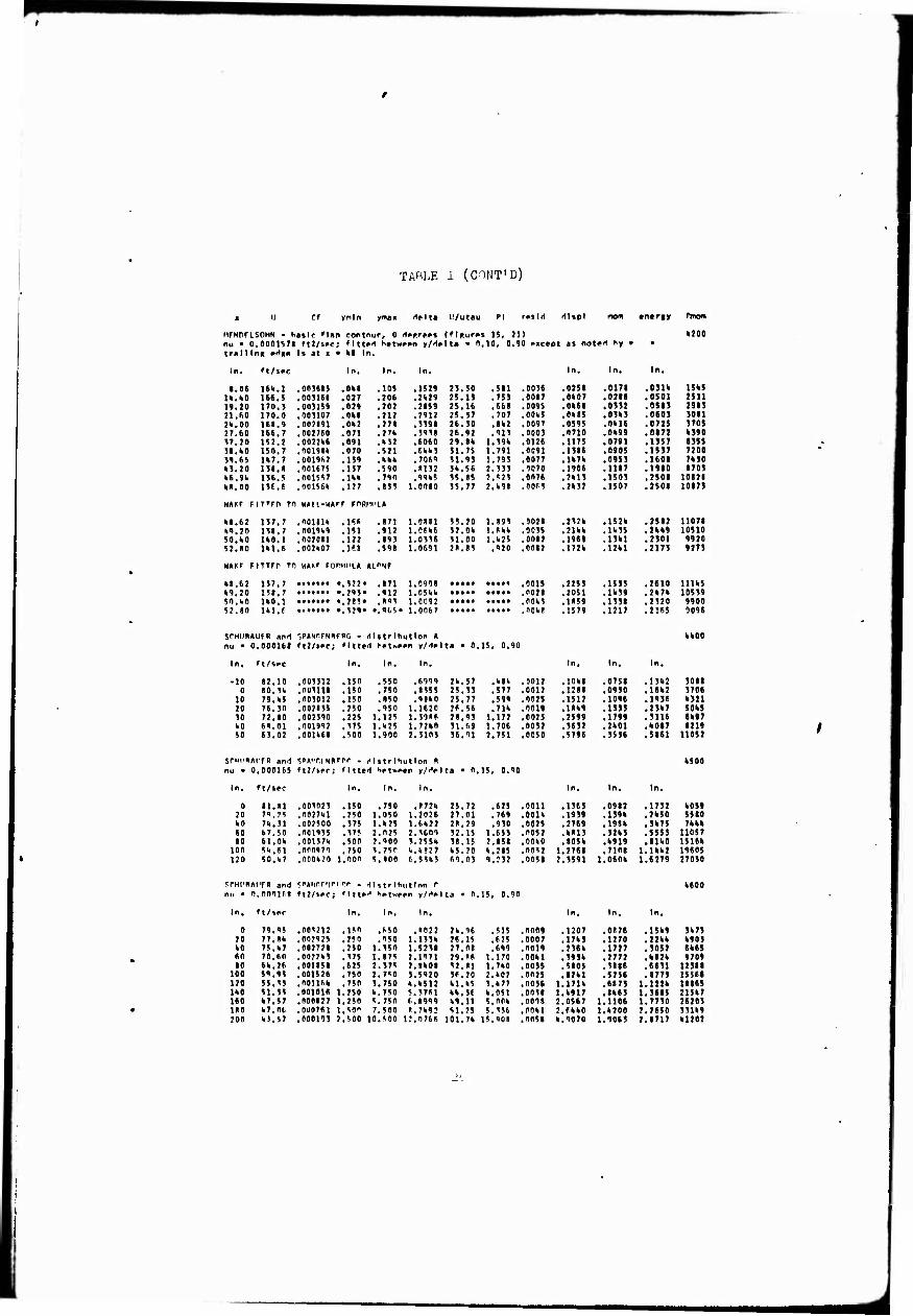
TABLE 1 (CONT'D)

ii rf ynfn ynai H»U» U/utau PI rrslH Hlspl mom eneriy

MFNmSOHN - hailc flap contour, 0 if>iir»»t (fliturvs IS, 21) nu • 0,00aiS7l ftl/irc; 'Ittod h«twi'i>n y/rf*)ta • 1,10, 0,90 nc»pt as notart ^y • tratllnK rrige It at ■ • »I In.

In. ft/»PC In, In, In, In. In. In,

Pmoffl

moo

1.0« ,0O)6IJ ,0k8 ,105 1529 25,50 ,511 .0056 0251 .0171 .0)16 1565 lll.H0 ,005161 .027 ,206 2k29 25.1) ,75) .0087 ,0k07 ,0286 ,0501 2511 19.20 ,005159 ,029 2859 25.16 ,668 .0095 0k6« ,0)52 ,051) 298) 21,ÜO ,005107 .Okl 2912 25.57 .707 .00k5 ,0k8S ,05k) .080) 5081 211.00 ,002891 ,0k2 5598 26,50 .8k2 .0097 0595 ,0616 .0725 5705 27,60 ,002760 .071 595« 26.92 .915 .000) 0710 ,0699 .0172 6)90 ?7.20 ,0022k6 .091 6060 29,8k 1.59k ,0126 1175 ,0791 .1)57 «555 31,kO ,00191k ,070 ,ekk5 )1,75 1,791 ,0091 1)8« .0905 .15)7 7200 59,S5 ,0019f>2 .159 7069 51.9) 1,795 .0077 lk7k .0455 ,1608 7k 50 k),20 ,001675 ,157 «152 5k,56 2.555 .0070 1906 .1187 ,1980 870) ke,9li IM.i ,001557 .Ikk 99k5 )5.«5 2,525 ,0076 2kl) .1505 ,2)08 10828 kn.eo U6.6 ,n0156k .127 1 0080 )S,77 2,k9« ,oor5 2k52 .1507 .2508 1087)

HAKF FITTm Tf W«ll-WArr FORI'I'l»

ill,62 157.7 .noiiik .166 ,171 1 0881 )),20 1,«95 ,0028 252k .152k .2582 11078 li9.2D 151.7 ,0019k9 .151 ,912 1 C6k6 )2,0k l,fkk .0055 2Ikk .lk55 .2669 10510 50,1.0 IkO.l ,002081 .122 .895 1 0556 51,00 l,k25 .0012 19« ,l)kl .2)01 9920 52,»0 1H.6 ,002k07 .16« ,59« 1 0691 21,«5 .920 .0012 172k ,12kl .217) 9275

NAICF FITTrr Tr W«ICF Fnnma* AlOHF

■■1,62 157.7 •.522« ,871 1 099« .0015 225) ,15)5 ,2610 nus k9,20 158.7 •,295» ,912 1 OSkk • •••• • •••« .0028 2051 ,lk)9 ,2k7k 10559 50,140 UO.l •,215» ,«95 1 0092 • •••• •*♦•* ,00k5 1«59 ,1558 ,2520 9900 52,«0 Ul.f •,529. • .915« 1 0067 .nokt 1579 ,1217 .2165 009«

SrHUKAUER and '.PANrfNUFBG - Hlttrlbutlon A kkOO nu • 0 .O00UI ft2/»»c; »Itt« <1 bat^aan y/Halta • 0. 15, 0.90

In, ft/i»c In, In, In, In, In, In,

-10 82,10 ,005512 .150 ,550 ,6999 2k,57 .kSk ,0012 lOkB ,0758 5088 0 80.5k ,005111 .150 ,750 ,8555 25,55 ,577 ,0012 128« .09)0 570«

10 79,k5 ,005012 .150 ,150 9860 25,77 ,599 ,0025 1512 ,109« k)21 20 76.50 ,002855 .250 .950 1 1620 26.56 .71k ,0019 18k9 ,1))) 5065 50 72,10 ,002590 .225 1.125 1 ,59«f 2«,95 1,172 ,0025 2599 .179» «697 kO 69.01 ,001992 .575 l.k25 1 72kfl 11,69 1.706 ,0052 56)2 .2601 8219 50 65,02 .00U6I ,500 1.900 2 510) 56,91 2.751 ,0050 5796 .)55« 11052

Srwl'^AlTR and SPMTINB'Pr . dljtrlSutlon H nu • 0,000165 ft2/ifr; fitted Sat»aan y/dalta ■ 0,15, 0,90

In, ft/»ac In, In, In, In, In,

6500

0 «1 ,005025 ,150 750 ,»72k 72 625 • ooii ,156) .0982 6059 20 ?! ,0027kl .250 050 1,202« 01 769 ,001k ,19)9 .159k 5580 kO 51 ,002500 ,575 k25 l,6k22 29 950 .0025 ,2769 ,19Sk 7666 60 50 ,001955 .57« 025 2.5609 15 I 655 ,0052 .k«l) .52k) 11057 «0 Ok ,00157k ,500 900 5,255k 15 2 «58 ,00k0 ,105k .k919 15166

100 61 ,000979 ,750 75r k,k827 70 k 785 ,0052 1,27«« .7108 1 19605 120 k7 ,0n0k20 1,000 «00 6,55k5 69 05 9 ;j2 ,0058 2,5591 l,0«0k 1 270)0

k«00 11 - n,ooMH ft2/»ac fllla ̂ Hatwaan y/dalla • 0.15, 0,90

In. ft/iar In, In, In, In, In, In,

0 79,95 .005212 .150 .650 96 ,51! .0009 ,087« 5k7) 20 77,«6 ,007925 ,250 .950 15 ,625 ,0007 kO 75,67 ,00272« .250 1,550 0« ,699 ,0019 60 70.60 ,0022k5 ,575 1,875 «6 1,170 ,0061 80 66.26 ,001858 ,625 2,575 «1 1.760 ,00)5

100 59.9) ,001526 .750 2,750 20 2,k02 .0025 120 55.55 ,"01166 .750 5,750 k5 5,k77 ,00)6 IkO 51.55 ,00101« I .250 k,750 5t k,051 ,005« 160 67,57 ,000827 1 .250 5.750 r.',«999 69, 1« !,00k ,0098 1 1«0 k7,0t ,000761 I .«0" 7,500 «,7k92 51, 25 5.556 .OOkl 1 200 k5,57 ,000195 2 .500 10,500 1?,0766 101, 7k 15,90« ,0058 1

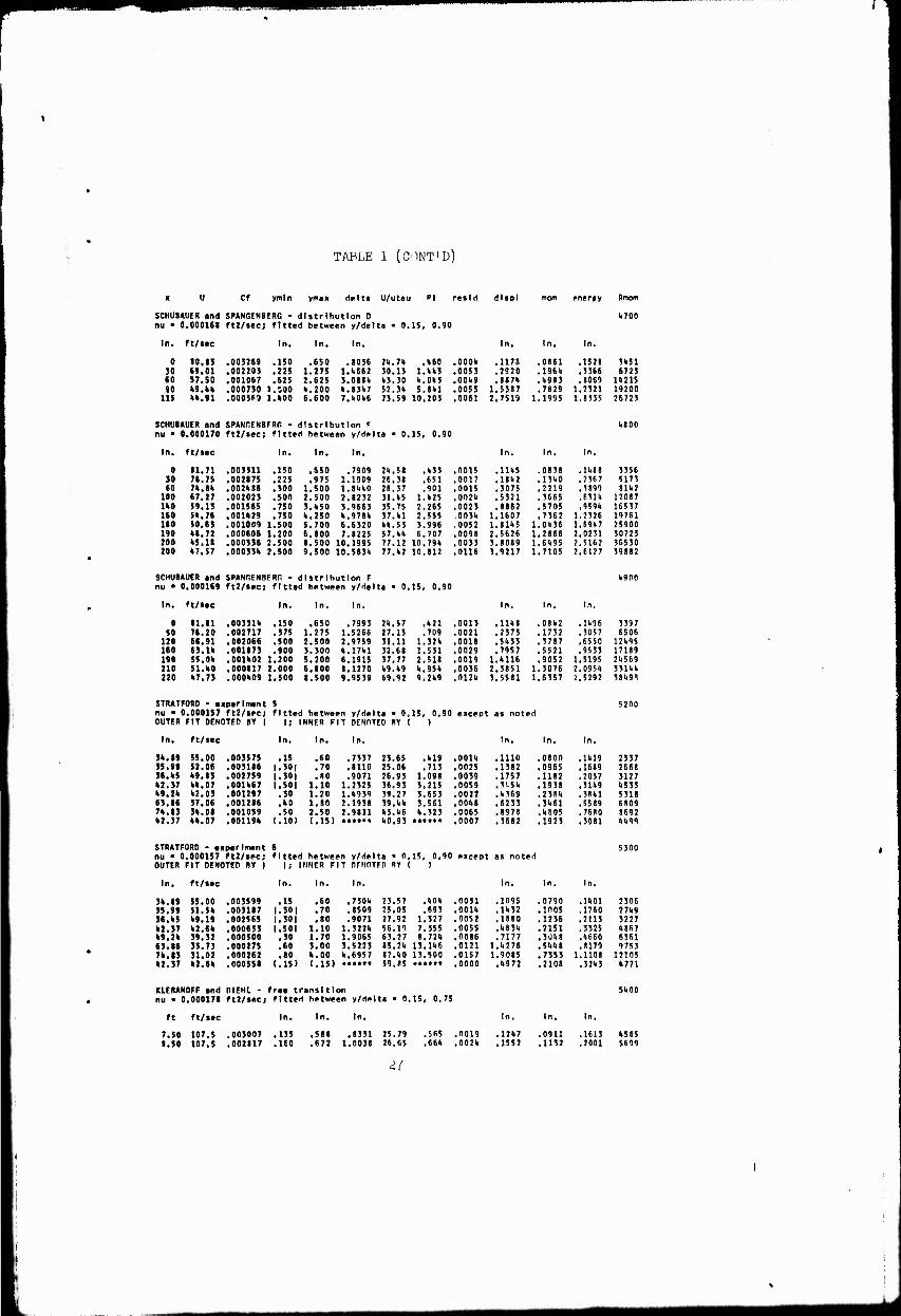
r

TABLE 1 (CONT'D)

Cf ymtn ytnax delta U/utau resld dlspl

SCHUBAUER and SPANGENBERG - distribution D nu • O.OOOIBi ft2/sec; fitted between y/delta • 0.15, 0,90

In. ft/««c In. In. In.

Rnom

Ii700

0 10.13 .003269 .150 650 .8036 .000» .117» .0861 .1521 3»51 30 69.01 .002203 .225 1 275 l.»662 1 .0053 .2920 .196» .3366 6725 «0 57.50 .001067 .625 ? 625 3.011» It .00»9 .817» .»983 .8069 1»21S 90 ii.hk .000730 1.S00 » 200 ».«J»7 5 .0055 1.5587 .7829 1.2321 19200 115 »».91 .000369 l.»00 6 600 7.»0»6 10 .0061 2.7519 1.1995 1.8535 26723

SCHUBAUER and SPANGENBERG - distribution F nu • 0.000170 ft2/sec; fitted between y/delta • 0.15, 0.90

In. ft/sec In. In. In. In. In. In.

»800

0 »1.71 .003311 .150 .650 .7909 »33 .0015 .11»5 0838 UI8 3356 30 7».75 .002875 .225 .975 1.1909 651 .0017 .I»»} 13»0 2367 5173 60 7».»» .002»I6 .300 1.500 1.8»»0 901 .0015 .3075 .2219 3899 8U2

100 67.27 .002023 .500 2.500 2.8232 1 »25 .002» .5521 .3665 631» 12087 no 59.13 .001565 .750 3.»50 3.9663 2 265 .0023 .8862 .5705 959» 16537 160 5».76 .001»29 .750 ».250 ».971» 2 555 ,005» 1.1607 .7362 2326 19761 110 50.63 .001009 1.500 5.700 6.6320 3 996 .0052 1.81»5 1 .0»36 69147 25900 190 »».72 .000606 1.200 6.800 7.8225 e 707 .009» 2.5626 1 .2866 0231 30723 200 »5.18 .000336 2.500 8.500 10.1995 10 79» .0033 3.8089 1 .6»95 5162 36530 200 »7.57 .00033» 2.500 9.500 10.583» 10 812 .0116 3.9217 1 .7105 6127 39882

CHUB AUEft and SPANGENBERG - dlstrlh utlon F »900 u • 0.000169 ft2/»ec. fitted between y/delta • 0 15 0.90

In. ft/»ac In. In. In. In. In. In.

0 »1.11 .00331» .150 .650 .7993 »21 .0013 .11»8 08»2 1»96 3397 50 76.20 .002717 .375 1.275 709 .0021 .2375 1732 3057 6506

120 66.91 .002066 .500 2.500 32» .001» .5»33 3787 6550 12»95 160 63.1» .001173 .900 3.300 531 .0029 .7957 5521 9533 17189 190 55.0» .001»02 1.200 5.200 51» .0019 l.»116 9052 1 5195 2»S69 210 51.»0 .000117 2.000 6.100 95» .0036 2.3851 1 .3076 2 095» 331»» 220 »7.73 .000*09 1.500 8.500 2»9 .012» 3.5581 1 .6357 2 5292 381.93

STRATFORD • experiment S nu • 0.000157 ft2/sec; fitted between y/delta • 0.15, 0.90 except as noted OUTER FIT DENOTED BY I I; INNER FIT DENOTED RY ( )

In. ft/see In. In. in. In.

55.00 .003575 .15 60 .7337 23.65 .001» .1110 .0800 .1»19 2337 52.06 .003116 |.30| 76 .8110 25.06 .0025 .1382 .0965 .1689 2668 »9.83 .002759 |.30| 80 .9071 26.93 .0039 .1757 .1182 .2037 3127 »».07 .001»67 l.50| 10 1.2325 36.93 .0059 .3i'5» .1938 .31»9 »533 »2.03 .001297 .30 20 l.»939 39.27 .0022 .»369 .238» .38»! 5318 37.06 .001216 .»0 80 2.1938 39.»» .00»8 .6233 .3»61 .5589 6809 3».01 .001059 .50 50 2.9811 »3.»6 .0065 .8978 .»805 .7680 8692 »».07 .00119» (.10) ,15) •*•*•• »0.93 .0007 .3682 .1923 .3081 »»99

STRATFORD - experiment nu • 0,000157 ft2/sec; OUTER FIT DENOTED BY I

In, ft/see

fitted between y/delta • 0.15, I; iriNER FIT nrnnTFn RY (

In. In.

0.90 except as noted )

In. In.

5300

.003599 .15 60 .730» 23.57 .»0» .0031 .1095 .0790 .U01 2306

.003187 l.30| 70 .8509 25.05 .693 .001» .1»32 .1005 .1760 27»9

.002565 1.301 80 .9071 27.92 1.327 .0052 .1880 .1236 .2113 3227

.000633 1.50! 10 1.322» 56.19 7,355 .0055 .»83» .2151 .3325 »867

.000500 .30 70 1.9065 63.27 8,72» .0086 .7177 .3ü»8 .»660 6361

.000275 .60 00 3.5223 85.2» 13.1»6 .0121 l.»276 .S»»8 .8179 9753

.000262 .80 00 ».6957 87.»0 13.500 .0157 1.9085 .7353 1.1108 12105

.000558 (.15) 15) 59.85 .0000 .»972 .2108 .32»3 »771

KLEBANOFF and DIEHL - free transition nu • 0,000171 rt2/sec; fitted between y/delta • 0,15, 0,75

ft ft/tec In, In, In. In. In.

7.50 107,5 .003007 .135 .588 .8331 25.79 .565 .0019 .12»7 .0911 .1613 »585 8.50 107.5 .002817 .160 .672 1.0038 26.65 .66» .002» .1552 .1132 .2001 5699

2f

1

TABLE 1 (CnNT'D)

9.50 10.50

107.5 107.5

yiMn ynn« iif\t» U/utnu PI ruld dlipl

.002721

.002657 .101. .211 .950

1.11.82 1.51.2k

27.OB 27.1.1.

.69!

.695 ,0020 .0017

.1710

.2050 .1J0! .1509

.2J02

.2672 6556 7597

KLfRAHOFF and mfHl - O.Ok-Ind' rod nu - 0,000171. ft2/sec; fitted l»tv««n y/dclt« ■ 0.15, 0.75 »xc«pt fit noted hy •

ft ft/s^c In. In. In. In. In.

ClriACDFr ,in.l IMFlij . 0.:5-lnc^ rod nu • 0.000171. ft2/i»c; fitted hetwpfn y/dfita ■ 0.15, 0.75 except as noted nUTFF FIT nF'IOTFD RV | |; ICNf! FIT PEWTfC BY ( )

ft/SPC In, In. In, In, In.

KUWinFF and nUHL - 21. nesl screen nii ■ n.000170 ftl/sec; fitted hetueen y/dclta ■ 0.15, 0.75

ft ft/sec In. In. In. In.

KLFnAIKlFF and niFML - sandpaper, 55 't/sec nu ■ 0.000165 ft2/spr; fitted hptween y/delta ■ 0.15, 0.75 except as noted OUTFR FIT nrnnTEn PY | | ; IMIirP FIT PFt'OT^r HY ( )

ft ft/Sec In. In. In, In. In. In.

5500

17 107 .005611 .01.2 ,11.0 .201.5 .0020 .0595 .0262 .01.511 07 107 .005561. ..122« ,280 .5859 .0027 .0602 .01.20 .0757 17 107 .005I.SO .092 ,528 .1.81.9 .0020 .0721. .0528 .095! no 107 .005205 ,155 ,1.87 .6557 .0012 ,0975 .0712 ,1261.

50 io- .002968 ,155 ,606 .8595 .0019 ,1271. ,0951 ,161.9 n 50 10. .002581. ,215 1,01.0 1.1.192 .OOU .2197 .1615 ,2852

5600

1. 17 115,0 .000016 ,7171 1.75 .6558 556,55 69.781 .0061. .5078 .0825 1. 25 109.2 .ooosns ,2501 50f ,6771. 1.9,77 5.895 .0026 .2515 .1117 1. f.7 107.1. .002900 .5091 685 1,0110 25,81. .1.68 .0009 .11.50 .1069 ■. 17 107.f. ,005181. ,1.111 80b 1,1686 25,06 .220 ,0018 .11.18 .1091. 0 on 107.2 ,005255 ,I.UI 201 1,6801. 21.,79 -.021 ,0021 .1020 .1298 7 50 107.2 ,005015 ,550 1.52 1.9628 25,1.2 .01.1. ,1011. .1995 ,1590 H 50 107.2 ,007975 .589 590 2.2102 25,91. .100 ,0010 .2519 .181.5 9 50 107,? ,002851. .51.1 707 2.5061 26,1.7 .199 ,0021 .2606 .2061. 10598

10 50 107,2 ,00271.7 .1.06 781. 2,1.285 26,98 .288 ,0027 .2905 .2285 11755 li 17 115,1 ,000215 .099) 090) «*•••• 16.79 ,0000 ,2965 ,0915 1. 75 100.2 ,001200 .055) 095) *•••«• 1.0.85 .0015 .2252 ,11U5 1. f.7 107.1. ,005560 .095) 171) 21..1.0 .0129 .151.1. ,1055 5 17 107.6 ,005519 .096) 191.) 25.81. .0151 .1519 ,101.7 f, no 107.2 ,005588 .158) 256) 21».50 .0072 .1578 ,1271

5700

; 00 1*5,1. ,cr.26ir. .251 725 1 0510 26.65 1,051. ,0027 .2071. ,1590 .2589 2956

5 50 1.5,1. ,005202 .290 1 156 1 5521 21..96 ,512 .0020 ,2291 ,1665 .291.2 5558 l. 50 1.5,1. .005229 .272 1 296 1 7571. 21.,89 ,1.20 .0052 .21.65 .1818 .525! 5807 f. 50 1.5,1. ,005085 .1.11 1 595 2 lU! 25,1.7 ,1.58 .0007 .2999 .2226 .5967 Ii7!7

10 50 1.5,1. ,002890 .511 1 188 2 8281 26,51 ,500 .0055 .5961. ,2960 .5276 6298

5800

2.08 .002179 .5101 701. 1.0127 50 21 1.187 ,0062 .21.81 .11.97 ,21.92 2685 2.5n ,002578 .5001 70! 1.1225 21 00 1,650 ,0010 .251.1. .1591. ,2682 2858

5,00 ,002721. .5081 800 1.2785 27 10 1,160 .001.5 .2501. ,1656 ,2851. 2969

i.,no ,005019 .507 095 1.5520 25 7U .765 ,0052 .2591 .1811 .5160 521.6

5.00 ,005065 .501 211. 1.71.1.7 75 55 ,658 ,0022 .2800 .1198 .5515 5585

5.50 .00501.9 .508 591 1.8907 25 61 ,652 ,0021. .291.7 .2112 .5715 5786

6,50 .005069 .1.06 591 2.101« 25 55 ,560 ,0018 .5171. .2511 .1.090 1.11.5

7,50 .002981 .1.06 687 2,189» 25 10 ,625 .0016 .51.05 .21.72 .1.565 1.1.52

8,50 .002959 .1.05 681. 2.5702 26 00 ,605 .00U1 .5628 .261.2 ,1.675 1.757

9,50 .00291.1 .1.08 687 2.5701 26 08 ,582 .0016 .5858 .2829 ,5011 507! 10,50 .002887 .605 981 2.71.52 ?f 52 ,601. .0021. .1.158 .5057 ,5581 51.1.5 2.08 .001852 .115) 115) 52 87 ***** .0000 .2581 .11.15 ,21.65 2676

2,50 .002570 .112) 152) 27 90 ***** .0028 .2506 .1595 ,2610 2857 5,00 .002878 .111) 151) 26 56 .0008 .21.75 .1655 ,2857 29(4

KIFRANOFF and niri'L - sandpaper, 55 ft/sec nu " 0,000166 ft2/5ec; fitted hptween y/delta - 0.15, 0.75 except as noted orTFO FIT rirnnTfp PY | [j INHFR FIT PFUOTFO OY ( )

ft ft/sec In. In. In. In. In, In,

2,08 55.1 .001858 1.5101 2.50 55.1 .002083 1.5081 5,00 55.1 .0021.65 1.5101

.701. ,1905 52 81 2 556 .0056 .21.85 .11.90 .21.68 U122

.702 1,1521. 50 91. 1 858 .OOIU .2559 .1606 .2692 1.1.1.2

,802 1,2162 28 1.8 1 21.5 .0011 .21.90 .1671 ,2861. 1.621

T/VHLK 1. (aniT'D)

u Cf ynln yn»« dolta I'/nttiu PI rmM HUpl mom Pnom

li.OO 5.00 5.SO 6,SO 7.SO 1,50 0,50

10,50 2,01 2,50 5.00

55,1 55,1 55,1 55,1 55,1 55,1 55,1 55,1 SS.l 55.1 55.1

,002645 ,002109 ,002857 .00281. U .0028115 ,002782 ,002760 .002726

,510 .52U .510 .14 or .1.06 .U0S .liOG ,li27

1.008 l.ll)2 1.196 1.591 1.587 I.Ml. 1.685 l.SSi.

.7605 ,«110 . Kf.l) .21.01 .«'JO .0150 751.«

.001591. (.071.) (,115) •••••. ,002505 <,111) (,151) ,002665 (,115) (.155)

77.21. 20.09 26.55 ?t.5l. 26,55 2C.«1 26.02 27.00 55.1.2 79.1.7 77.1.1

,«I.K ,68b .6 59 .505 .555 .559 ,51.5 .560

• •*•#

,"020 .0015 .0055 ,0008 .001U .0021 ,0010 .0019 .0021. .0005 .0020

.2f.6'l

.2765

.2811.

.5065

.'185

.51.81

.5705

.5(115

.2581

.2512 ,21.1.5

.18H9

.2006

.2060

.226«

.2568

.2595

.2771.

.2919

.use

.1605

.1665

.5500

.5557

.561.1.

.1.075

.1.210

. Ii 618

.1.91.5

.5202

.21.1.1

.2702

.2865

5221. 551.8 5097 6275 6550 7179 7672 8071. Uli 1.1.59 1.606

KLFPANOFF an(i PIFML - 5Än.(paper, 103 ft/irr nu • 0.000165 ft2/i«c; fitted ^rtvirrn v/^'\t!t • n,15, oiiTfn FIT nniorrn ov i i; in'ift> TIT nffrrrr «v (

0,75 except as note'' )

ft ft/»ec In. In. In. In.

2.08 108.5 .001661. .51.01 751. 1.0051. 51. 67 2.1^7 ."015 .21.15 .11.96 .21.92 8197

2.50 108.5 .001896 .21.21 751. 1.121.1 52 M 1.858 .0016 .21.28 .1580 .2672 E65 8 5.00 108.5 .002190 .51.01 952 1.509? 50 77 1.285 .0022 .71.07 .I0(.7 .7367 0106 li.OO ioa.5 .0021.72 .21.0 126 1.5885 ?y. kl. .noT .21.52 .Vt .»167 181.1 5.00 108.5 .002550 .505 111 1.1181 ?s on .nnio .2586 .1957 .Hkl. 10615 5.50 108.5 .002561 .51.0 525 1.8915 27 95 .OOi.O .265 5 .2001 .5565 10961. 6.50 108.5 .002561. .55« 1.21 2.K78 27 95 .0019 .28k? .2161 .5865 1181.5 7.50 108.5 .002550 .I.0U 58»i 2,2581 28 nn .0011 .5008 .2295 .1.117 12577 «.50 108.5 .00251.5 .1.55 5U, 2.1.571 2S Ok .0015 .5188 .21.1.8 .1.591. 151.11. 9.50 108.5 ,0021.92 .1.01. «80 2.5958 2a ^x .0022 .51.56 .2657 .1.750 lkU52

10.50 108.5 .0021.75 .505 802 2.71.1.1 78 1.5 .0006 .56 05 .7769 .1.975 15171 2.08 108.5 .001520 .065) 081.) 5C 12 **«*• .0005 .2560 ,11.91) .71.57 sm 2.50 108.5 .00201.9 .101.) US) 51 21. »«•*« .0011. .2595 .1570 .2677 8651

5.00 108.5 .00251.1 ,081.) 11.5) 29 25 **••« .0000 .2^61. .16511 .2861. 9C61.

BAUER - 20 rter.ree slnpe nu • 0,0000091.1. ft2/»ec; fitted hetieen v/4elta • n.15, 0.60 pxrept as note-1

ft/sec In. In.

5 8.51. .001.021. •,120. ..102. .2771 22 2') .155 .0012 0572 ."279 .0501. 2056

1. 9.68 .005555 •,006« ..2ii0. .1191. 25 79 .718 ."01.0 0515 ."589 .0700 1521.

5 10.«9 .0051.75 .072 .192 .5799 2 5 9') .71.1 .0018 "501 .0582 .0689 1071

6 12.06 .005215 .096 .788 .1.575 21. 91. .268 .0021. 0020 .01.71. .0853 501.0

7 12.85 .005128 .09G .28« .5111. 25 2'i .782 .0017 0668 .0511. .0978 5829

8 15.69 .005001 .096 .28« .5799 75 87 .11'. .0015 0758 .0587 .1060 7087

9 111.51 .002977 .096 .556 .6121 2C U .311. .0916 0815 .0651. .111.6 8117 10 15.26 .09281.7 .12" .1.52 .72';5 2f 51 .502 .0025 0902 .0701. .1275 91.86

11 15.97 ,002756 .120 ,1.52 ,71.9« 27 nu .182 .0022 0995 .0777 .11.05 1991.9

12 16.68 ,002711 .m .51.0 .8980 27 u. .29« .0016 1080 .0850 .151.2 12515

15 17.51 .002681 .lUk .51.0 .9560 27 M .292 .0026 1127 ,0691 .1620 15617

U 17.07 .0O2C1.9 ,U8 .6 00 1.0161. 77 1.8 .269 .0016 1176 .0933 .1698 11.805

15 18.58 ,002601. .192 .1.00 1.17RC 27 71 .251 .0015 urt .1021. .1865 10705

16 19.17 ,002575 .192 .r.nn l.uor, 27 St .265 .0921. 1290 .1025 .1361. 1751.0

BAUFR - 1.0 deftrce slope nu " 0.00001952 ft2/sec; fltte-l ^.rti.epn y/delta ■ 0.15, 0.60 except as noted >iy •

ft/sec In. In. In.

2 10 77 .001.075 «.081.. ,11.1. .2619 22 16 .059 .0"07 .0511. .0235 .0k21 2003 5 60 .001800 >.io«. .192 .5375 22 91| .012 .001« .0182 .0293 .0512 2027 1. 10 .003005 .072» .216 .5903 25 56 .01.2 .0022 .01.11 .053k .0606 3727 5 55 .00335« .072 .21." .1.587 71. 1.8 .121 .0025 .0520 .0k05 .0751 kOOO 6 8li .005091. .081. .7 76 .1.992 25 l.l .252 .0075 .9011. .0k7k .0357 6328 7 02 .002992 .090 .Ik« .6"11 25 86 .222 .0010 .0701 ,n5k6 .0988 7791 8 12 .007912 .096 .51.8 .6516 26 71 .21.6 .0016 .0755 .0580 .1067 8923 9 19 .002029 .120 .1*20 .7256 76 59 .255 .0019 .0631 .0652 .HBk 101.31

10 20 .002755 .120 .1.20 .7656 26 05 .265 .0017 ,0900 .0709 .1288 11913

11 09 .002686 .Ikh .1.68 .8155 27 70 .288 .0021 .0951. .0750 .1361 13131 12 08 .002613 .11.1. .516 .9 261 27 50 .263 .0011 . 101.8 .0850 .1508 15170

13 95 .002505 .168 .5611 1.0073 27 77 .250 .0011. .1113 .088k .1609 16778

u 79 .00251.3 .168 .612 1.0651. 28 05 .206 .1011 .1199 .0956 .17k2 18783

BAUFR - 60 deeree slope nu • 0.0000097k ft2/5ec; fitted Ketween y/delt« • 0.15, 0.60

ft ft/sec In.

2 13.88 .005165 .0k8

In. In. In. In. In.

.168 .5009 25.1k .k99 .0012 .0k61 .03kl .0607 kOke

29

M

TABLE 1 (CONT'D)

Cf ymln ymax delta U/ut«u PI msld dttpl mom entrity Rmom

is.n .003011 It .072 .5ii0 .14090 .390 .0011 .0550 .OI4IS 07143 5621 17.5J .005027 .072 .21.0 .14566 .523 .0012 .0573 .mi 0796 6611 11.91 .0029511 ,0814 .211 .149147 .312 .0015 .0623 .014112 0170 7826 20.14? .002151 .096 .336 .5716 .307 .0007 .0703 .05141 0991 9592 J1.7I .0027514 .096 .536 .i:075 .327 .0016 .0759 ,05914 1076 11072 25.02 .00266l( .101 .5111 .6769 .5147 .0016 .013« .0657 1U9 12953 2H.19 .0026511 .120 .1452 .75114 .3014 .0017 .01914 .0707 1213 1146214

10 JS.JI4 .002592 .HI. .UIO .1559 .279 .0013 .0976 .0771 nn 16860 11 26.59 .00251)9 .lltU .I4IO .16*2 .290 .0015 .10014 .0791 1*52 18021 12 27.It5 .002510 .Uk .5140 .9501 .2714 .OOU .1079 .0163 1575 20263

BRADSMAW - layer A (prohe ill tplncment correction removed) nu • 0.0001585 ft2/»ee; flttert hetween y/<<elt« • 0.10, 0.90 lour point it « • 72, y • 0.996 tuppressed In fitting

6I4OO

In. ft/sec In. In, In. In. In,

214 125,65 .002979 .051 .396 .1.668 25,91 .71.6 .0018 .0780 .0551 ,0966 36140 30 120,1.1 .00261.7 .076 .1496 .58146 27.1.9 1.007 .0022 .1057 .0753 ,1273 1)61414 56 11I..85 .002317 .106 .eiiF. .7668 29.58 1.317 .0020 .11.89 .1011 ,1738 142 110,76 .002110 .106 .796 .93147 50.79 1.5D8 .0015 .1901 .1268 ,2165 1.8 107,13 .002135 .106 .896 1.0592 30.61 1.1.72 ,001.7 .2061 .1591. ,2388 60 101,140 .n0203U .1146 1.196 1,3727 31.36 1.526 .0022 .2712 .1837 ,311.6 72 16.82 .001923 .196 1.51.6 1.71.10 32.25 1.625 .0016 .3515 .2379 .I4OEI4 12110 to 92.<)5 .0018149 .2146 1.896 2,1523 32.89 1.682 .0021. ,143011 ,2911 .14977 1(4225

BRAPSHAW • layer R (prohe displacement correction removed) nu • 0,0001562 ft2/sec; fitted between y/delta • 0.10, 0.90 sour point at x ■ I48, y ■ 0.996 suppressed In fitting

6500

In. ft/see In. In, In. In. In.

214 125.63 .002686 .076 .6146 .7196 7,29 .830 .0055 .081.8 .1 81) 5682 30 120.1.8 .002510 .796 .8956 8.23 .952 .0013 .1085 .1 95 6976 36 1114.85 .002233 .91.6 1.0661 9.93 1.267 .0022 .1573 .2' 75 81)13 142 110.76 .002051 1.096 1.2583 1,23 1.1.89 .0021 .1675 .2 71) 9899 «a 107.13 .001968 1.196 1.14311 1,88 1.585 .0019 .1907 .3 61) 10902 60 101.1)0 .001818 1.596 1.8229 3,16 1.775 .0027 .21.92 .14 1)8 131)82 72 96.82 .001685 1.91.6 2.2051 14,145 1.986 .0022 .5082 .5 21) 15919 8I4 92.95 .001652 2.296 2,5996 (14,79 1.998 .0028 5500 .3632 .6 72 18010

30

■R

I

k

Notes for figure 1:

(a) flow 1600 (Riabouchinsky 1914); last 5 profiles; complete profiles are at x = 4, 10.94 m.

| (b) flow 2200 (Clauser 1954, flow 1); 8 profiles, renormalized; complete profiles are at x = 83,

I 327 in. j

(c) flow 2500 (Bradshaw 1966, a = -0.150); round pitot tube (displacement correction removed); 4 profiles; complete profiles are at x = 24, 84 in.

I (d) flows 6100, 6300 (Bauer 1951, 20°, 60° slope); last 10, 8 profiles; complete profiles are at x = 7 ft, 20° slope and at x = 12 ft, 60° slope.

( (e) flows 1100, 1200 (Ludwieg and Tillmann 1949,

! moderate or strong positive pressure gradient); last 10, 8 profiles (except x = 3.932 m omitted,

, flow 1200); complete profiles are at x = 1.782 m, moderate gradient and at x = 3.732 m, strong gradient.

(f) Preston-tube calibration in pipe flow (Patel 1965).

Notes for figure 3:

(a) flow 2300 (Clauser 1954, flow 2); 8 profiles; n ~ 4.13.

(b) flow 2600 (Bradshaw and Ferries 1965, a = -0.255); flat pitot tube; 4 profiles; n ~ 2.99.

(c) flow 2600a (Bradshaw 1966, a = -0.255); round pitot tube (displacement correction removed); 2 profiles, 11 ~ 2.99. One sour point suppressed in fitting.

(d) flow 2200 (Clauser 1954, flow 1); 8 profiles, renormalized; n ~ 1.71.

(e) flow 2500 (Bradshaw 1966, a = -0.150); round * pitot tube (displacement correction removed);

4 profiles; H ~ 1.20.

Notes for figures 4 and 5:

• (a) flow 1400 (Wieghardt 1944, constant pressure); ,, last 15 profiles; Fl ~ 0.62.

(b) flows 5400, 5500,5800, 5900 (Klebanoff & Diehl 1951); last 4, 2, 4, 4 profiles; 11 ~ 0.60.

(c) flows 6100, 6300 (Bauer 1951, 20°, 60° slope); small pitot tube; last 10, 8 profiles; n ~ 0.30.

I 31

'

(d) flow 6200 (Bauer 1951, 40 slope) ; large pitot tube; last 9 profiles; U ~ 0.26.

(e) flow 1300 (Ludwieg and Tillmann 1949, dp/dx < 0); last 8 profiles; H ~ 0.24.

Notes for figure 6:

(a) flows 5200, 5300 (Stratford 1959, experiments 5 and 6) ; last 3, 3 profiles.

(b) flow 3500a (Newman 1951) ; 7 profiles (turbulence correction removed).

(c) flow 2900 (Perry 1966); 10 profiles (last profile incomplete).

(d) flows 1100, 1200 (Ludwieg and Tillmann 1949, moderate or strong positive pressure gradient) ; last 10, 8 profiles (7. > 1) (except x = 3.932 m omitted, flow 1200).

(e) flows 6400, 6500, 3300 (Bradshaw 1967, 3=0- -0.255, layers A, B, C); displacement correction removed; last 7, 6, 6 profiles (11 > 1) . Two sour points suppressed in fitting.

Notes for figures 8 and 9:

(a) flows 1700, 1800 (Gruschwitz 1931, Messreihe 4, 5); profiles for 59.3 < x ^ 71.7 cm, 84.35 < x < 96.7 cm (11 > 1) .

(b) flow 3200 (Bell 1966, flow E); last 7 profiles (H > 1).

(c) flow 3000 (Bell 1966, constant pressure); last 9 profiles; R ~ 0.63.

(d) flow 1500 (Tillmann 1945, ledge); last 6 profiles; H ~ 0.09.

(e) flow 1600 (Riabouchinsky 1914); last 5 profiles (data incomplete at outer edge of layer); n ~ 0.85.

10,000

Figure 1, Data from several sources in the coordinates of the law of the wall. The lowest curve (f) is Patel's (1965) Preston-tube calibration in pipe flow. Each of the other curves shows all of the data points near the wall which were not used in the fitting operation, together with two complete profiles for reference.

33

M

m

20

H 32

15

10. 10 15 20 2.5

Figure 2. Evaluation of integral thicknesses by different methods. Curve (a) shows values obtained by Coles and Hirst, using parabolic interpolation in the sublayer (cf Volume II of the proceedings of this conference). Curve (b) is the same except for omission of data for which the profile is not experimentally defined near the wall. Curve (c) again shows all of the data, as in curve (a), but with values obtained using a standard sublayer profile (cf Table I of this survey). The solid lines correspond to equations (l)-(3), which assume a logarithmic profile in the sublayer.

3H

CLAUStH HOW?

*»

W I

£. f rt ■ —►

BHAObMAW 8 FfRRISS a= .?e.b (FPI

BRAOSHAW 0-.255 (RP1

CLAUStR FLOW I

BRAOSHAW o .150

Figure 3. The wake component for equilibrium flow in a positive pressure gradient. The vertical bars show the limits of the fitting region and_also show the relative size of a velocity increment of 0.01 U». Points with yuT/v < 50 are omitted.

M

F

s

y

■S-'

:>*■

S"

WltGHARDT 33 m/s

KLLBANOFF & DIEHL

I i _.-• i

r I \...

^4< 0

i

1 .5

y/8

- .a~. " • -J?

BAUER 20°, 60°

Figure 4. The wake component for equilibrium flow in a zero or negative pressure gradient. The vertical bars show the limits of the fitting region and_al8o show the relative size of a velocity increment of 0.01 U». are omitted.

Points with yuT/v < 50

J"

AÖ

Wit GHARl T

31 ms

f -. —•

" *• ■»*

KLtBANOM ft DitH.

BAUE K ?Q°, 60°

BAU! K 40"

'., • -

LUDWif G H Tin MANN

dp dx

vO

-.51—

I .5 1.0 I.S

y/8

Figure 5. The data of figure 4 replotted as residuals to emphasize discrepancies near the wall and near the free stream. The vertical bars show the limits of the fitting region and also show the relative size of a velocity increment of 0.01 Go,. Points with yuT/v < 50 are omitted.

i(

.

STRATFORD EXP 5,6

\M <

Figure 6. The wake component for several flows of airfoil or diffuser type. The vertical bars show the limits of the fitting region. Points with yuT/v < 50 are omitted.

38

8.5-18.0 FT 7

Figure 7. The measurements by Schubauer and Klebanoff (1950) (flow 2100), analyzed separately for (a) the upstream region of flow over a plane surface, and (b) the downstream region of flow over a curved surface of large radius. The vertical bars show the limits of the fitting region. Points with yuT/v < 50 are omitted.

39

GRUSCHWITZ -7 /

Zr-

"0 >-.'

Figure 8. The wake component for several flows showing small anomalies. The vertical bars show the limits of the fitting region, and for the two lower curves also show_the relative size of a velocity increment of 0.01 ÜB (0.01 Üw in the case of Riabouchinsky's experiment). Points with yuT/v < 50 are omitted.

u

AU

GRUSCHWITZ

■ ■ ■■^■.—

^ y^^ttffÄU*»»^*^^ f^Ä^rr-.y

.■"^^-i—,^.'—'

TILLMANN LEDGE -

Nt^.-—- -

RIABOUCHINSKY

e

y/S 1.0 1.5

Figure 9. The data of figure 8 replotted as residuals to emphasize the various anomalies. The vertical bars show the limits of the fitting region, and for the three lower curves also show the relative size of a velocity increment of 0.01 0« (0.01 Uw in the case of Riabouchinsky's experiment). Points with yuT/v < 50 are omitted.

41

ff

i H

////////////////.

Ftni

Figure 10. The local friction law F(K). The insert shows the complete analytical curve defined by equations (11) and (12) , assuming a logarithmic profile in the sublayer. The data in (a) are placed according to equations (9) and (10), using values of H, f, and R. * fr'om Table I. The data in (b) are adjusted by reducing 5* by 65 v/Ü» in both H and Rfl*.

\2

r

004

Cf 30(6100,6300)

62(14001

20000

a

40000

004-

JOOOO

n-o n= 62

n-299

The development of several flows in the coordinates Figure 11 cf , puted from equations (9) and (10) with 6* reduced by 65v/Uoo in both H and R&*.

Rg . The solid lines representing equilibrium flow are com-

6100/6300 1400 2500 2200 2600, 2600a 2300

5800/5900/6000 5600 1500 6400/6500/3300 2400

Bauer (1951), 20O/60O slope Wieghardt (1944), constant pressure Bradshaw (1966), a = - 0.150 Clauser (1954) , flow 1 Bradshaw and Ferriss (1965), a = - 0.255 Clauser (1954), flow 2

Klebanoff and Diehl (1951), sand, 35/55/108 ft/sec Klebanoff and Diehl (1951), 1/4-inch rod Tillmann (1945), ledge Bradshaw (1967), layers A/B/C Bradshaw and Ferriss (1965), a = - 0.255 - 0

!0

Figure 12. Comparison of the wake component for the equilibrium flow a = - 0.255 (flow 2600) and the corresponding relaxing flow a = - 0.255 - 0 (flow 2400) of Bradshaw and Ferriss (1965).

t i

r

0|-

NORMALIZED VELOCITY

DEFECT IN WAKE

OR IN EQUIVALENT

WAKE

1.0

n

PROCESSED AS BOUNDARY LAYER

o —CL-A

/ ft

9

PROCESSED

AS WAKE

1 1

.5-

.5 X/t

10

Figure 13. Relaxation process near the trailing edge of an airfoil (Mendelsohn 1947)(flow 4200). The circles show the velocity defect at the wall for the equivalent wake, as established by a boundary-layer fit. The triangles show the velocity defect at the plane of symmetry, as established by a wake fit. The squares show the actual velocity at the plane of symmetry in the wake.

^

i tiib young person's guide to the data a survey lecture

Documents