375

Chapter

17Cluster Analysis

Identifying groups of individuals or objects that are similar to each other but different from individuals in other groups can be intellectually satisfying, profitable, or sometimes both. Using your customer base, you may be able to form clusters of customers who have similar buying habits or demographics. You can take advantage of these similarities to target offers to subgroups that are most likely to be receptive to them. Based on scores on psychological inventories, you can cluster patients into subgroups that have similar response patterns. This may help you in targeting appropriate treatment and studying typologies of diseases. By analyzing the mineral contents of excavated materials, you can study their origins and spread.

Tip: Although both cluster analysis and discriminant analysis classify objects (or cases) into categories, discriminant analysis requires you to know group membership for the cases used to derive the classification rule. The goal of cluster analysis is to identify the actual groups. For example, if you are interested in distinguishing between several disease groups using discriminant analysis, cases with known diagnoses must be available. Based on these cases, you derive a rule for classifying undiagnosed patients. In cluster analysis, you don’t know who or what belongs in which group. You often don’t even know the number of groups.

Examples

You need to identify people with similar patterns of past purchases so that you can tailor your marketing strategies.

You’ve been assigned to group television shows into homogeneous categories based on viewer characteristics. This can be used for market segmentation.

376

Chapter 17

You want to cluster skulls excavated from archaeological digs into the civilizations from which they originated. Various measurements of the skulls are available.

You’re trying to examine patients with a diagnosis of depression to determine if distinct subgroups can be identified, based on a symptom checklist and results from psychological tests.

In a Nutshell

You start out with a number of cases and want to subdivide them into homogeneous groups. First, you choose the variables on which you want the groups to be similar. Next, you must decide whether to standardize the variables in some way so that they all contribute equally to the distance or similarity between cases. Finally, you have to decide which clustering procedure to use, based on the number of cases and types of variables that you want to use for forming clusters.

For hierarchical clustering, you choose a statistic that quantifies how far apart (or similar) two cases are. Then you select a method for forming the groups. Because you can have as many clusters as you do cases (not a useful solution!), your last step is to determine how many clusters you need to represent your data. You do this by looking at how similar clusters are when you create additional clusters or collapse existing ones.

In k-means clustering, you select the number of clusters you want. The algorithm iteratively estimates the cluster means and assigns each case to the cluster for which its distance to the cluster mean is the smallest.

In two-step clustering, to make large problems tractable, in the first step, cases are assigned to “preclusters.” In the second step, the preclusters are clustered using the hierarchical clustering algorithm. You can specify the number of clusters you want or let the algorithm decide based on preselected criteria.

Introduction

The term cluster analysis does not identify a particular statistical method or model, as do discriminant analysis, factor analysis, and regression. You often don’t have to make any assumptions about the underlying distribution of the data. Using cluster analysis, you can also form groups of related variables, similar to what you do in factor analysis. There are numerous ways you can sort cases into groups. The choice of a method depends on, among other things, the size of the data file. Methods commonly used for small datasets are impractical for data files with thousands of cases.

377

Cluster Analysis

IBM SPSS Statistics has three different procedures that can be used to cluster data: hierarchical cluster analysis, k-means cluster, and two-step cluster. They are all described in this chapter. If you have a large data file (even 1,000 cases is large for clustering) or a mixture of continuous and categorical variables, you should use the IBM SPSS Statistics two-step procedure. If you have a small dataset and want to easily examine solutions with increasing numbers of clusters, you may want to use hierarchical clustering. If you know how many clusters you want and you have a moderately sized dataset, you can use k-means clustering.

You’ll cluster three different sets of data using the three IBM SPSS Statistics procedures. You’ll use a hierarchical algorithm to cluster figure-skating judges in the 2002 Olympic Games. You’ll use k-means clustering to study the metal composition of Roman pottery. Finally, you’ll cluster the participants in the 2002 General Social Survey, using a two-stage clustering algorithm. You’ll find homogenous clusters based on education, age, income, gender, and region of the country. You’ll see how Internet use and television viewing varies across the clusters.

Hierarchical Clustering

There are numerous ways in which clusters can be formed. Hierarchical clustering is one of the most straightforward methods. It can be either agglomerative or divisive. Agglomerative hierarchical clustering begins with every case being a cluster unto itself. At successive steps, similar clusters are merged. The algorithm ends with everybody in one jolly, but useless, cluster. Divisive clustering starts with everybody in one cluster and ends up with everyone in individual clusters. Obviously, neither the first step nor the last step is a worthwhile solution with either method.

In agglomerative clustering, once a cluster is formed, it cannot be split; it can only be combined with other clusters. Agglomerative hierarchical clustering doesn’t let cases separate from clusters that they’ve joined. Once in a cluster, always in that cluster.

To form clusters using a hierarchical cluster analysis, you must select:

A criterion for determining similarity or distance between cases

A criterion for determining which clusters are merged at successive steps

The number of clusters you need to represent your data

Tip: There is no right or wrong answer as to how many clusters you need. It depends on what you’re going to do with them. To find a good cluster solution, you must look at the characteristics of the clusters at successive steps and decide when you have an interpretable solution or a solution that has a reasonable number of fairly homogeneous clusters.

378

Chapter 17

Figure Skating Judges: The Example

As an example of agglomerative hierarchical clustering, you’ll look at the judging of pairs figure skating in the 2002 Olympics. Each of nine judges gave each of 20 pairs of skaters four scores: technical merit and artistry for both the short program and the long program. You’ll see which groups of judges assigned similar scores. To make the example more interesting, only the scores of the top four pairs are included. That’s where the Olympic scoring controversies were centered. (For background on the controversy concerning the 2002 Olympic Winter Games pairs figure skating, see http://en.wikipedia.org/wiki/2002_Olympic_Winter_Games_figure_skating_scandal. The actual scores are only one part of an incredibly complex, and not entirely objective, procedure for assigning medals to figure skaters and ice dancers.)*

Tip: Consider carefully the variables you will use for establishing clusters. If you don’t include variables that are important, your clusters may not be useful. For example, if you are clustering schools and don’t include information on the number of students and faculty at each school, size will not be used for establishing clusters.

How Alike (or Different) Are the Cases?

Because the goal of this cluster analysis is to form similar groups of figure-skating judges, you have to decide on the criterion to be used for measuring similarity or distance. Distance is a measure of how far apart two objects are, while similarity measures how similar two objects are. For cases that are alike, distance measures are small and similarity measures are large. There are many different definitions of distance and similarity. Some, like the Euclidean distance, are suitable for only continuous variables, while others are suitable for only categorical variables. There are also many specialized measures for binary variables. See the Help system for a description of the more than 30 distance and similarity measures available in IBM SPSS Statistics.

Warning: The computation for the selected distance measure is based on all of the variables you select. If you have a mixture of nominal and continuous variables, you must use the two-step cluster procedure because none of the distance measures in hierarchical clustering or k-means are suitable for use with both types of variables.

* I wish to thank Professor John Hartigan of Yale University for extracting the data from www.nbcolympics.com and making it available as a data file.

379

Cluster Analysis

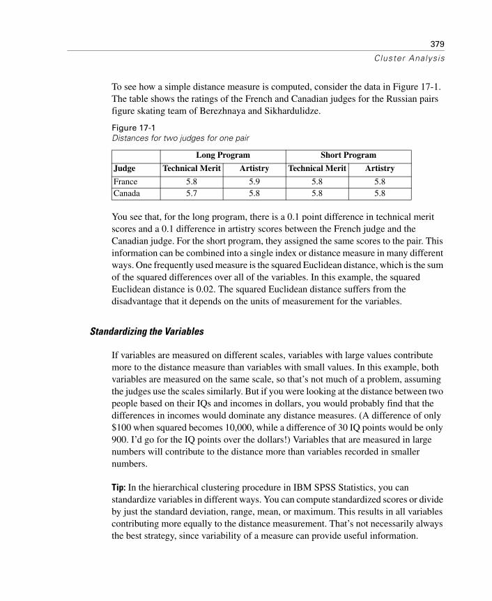
To see how a simple distance measure is computed, consider the data in Figure 17-1. The table shows the ratings of the French and Canadian judges for the Russian pairs figure skating team of Berezhnaya and Sikhardulidze.

Figure 17-1Distances for two judges for one pair

You see that, for the long program, there is a 0.1 point difference in technical merit scores and a 0.1 difference in artistry scores between the French judge and the Canadian judge. For the short program, they assigned the same scores to the pair. This information can be combined into a single index or distance measure in many different ways. One frequently used measure is the squared Euclidean distance, which is the sum of the squared differences over all of the variables. In this example, the squared Euclidean distance is 0.02. The squared Euclidean distance suffers from the disadvantage that it depends on the units of measurement for the variables.

Standardizing the Variables

If variables are measured on different scales, variables with large values contribute more to the distance measure than variables with small values. In this example, both variables are measured on the same scale, so that’s not much of a problem, assuming the judges use the scales similarly. But if you were looking at the distance between two people based on their IQs and incomes in dollars, you would probably find that the differences in incomes would dominate any distance measures. (A difference of only $100 when squared becomes 10,000, while a difference of 30 IQ points would be only 900. I’d go for the IQ points over the dollars!) Variables that are measured in large numbers will contribute to the distance more than variables recorded in smaller numbers.

Tip: In the hierarchical clustering procedure in IBM SPSS Statistics, you can standardize variables in different ways. You can compute standardized scores or divide by just the standard deviation, range, mean, or maximum. This results in all variables contributing more equally to the distance measurement. That’s not necessarily always the best strategy, since variability of a measure can provide useful information.

Long Program Short Program

Judge Technical Merit Artistry Technical Merit Artistry

France 5.8 5.9 5.8 5.8Canada 5.7 5.8 5.8 5.8

380

Chapter 17

Proximity Matrix

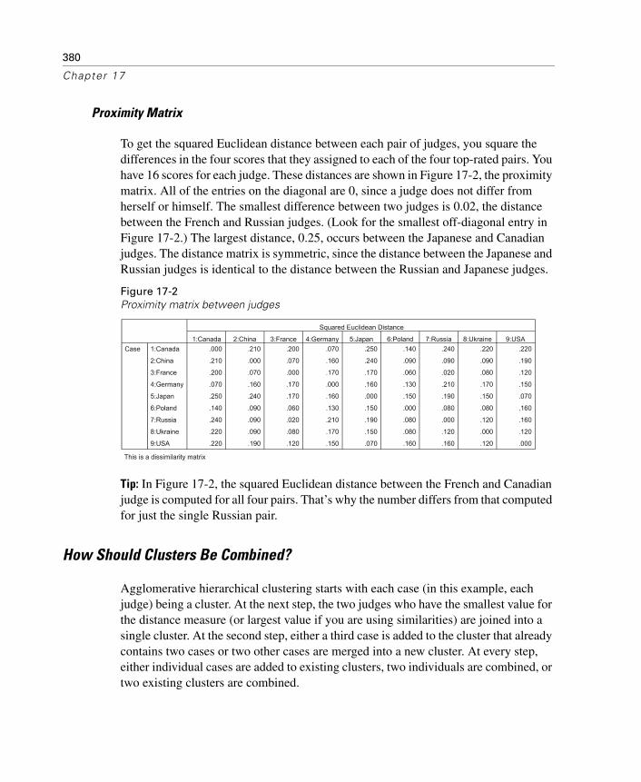
To get the squared Euclidean distance between each pair of judges, you square the differences in the four scores that they assigned to each of the four top-rated pairs. You have 16 scores for each judge. These distances are shown in Figure 17-2, the proximity matrix. All of the entries on the diagonal are 0, since a judge does not differ from herself or himself. The smallest difference between two judges is 0.02, the distance between the French and Russian judges. (Look for the smallest off-diagonal entry in Figure 17-2.) The largest distance, 0.25, occurs between the Japanese and Canadian judges. The distance matrix is symmetric, since the distance between the Japanese and Russian judges is identical to the distance between the Russian and Japanese judges.

Figure 17-2Proximity matrix between judges

Tip: In Figure 17-2, the squared Euclidean distance between the French and Canadian judge is computed for all four pairs. That’s why the number differs from that computed for just the single Russian pair.

How Should Clusters Be Combined?

Agglomerative hierarchical clustering starts with each case (in this example, each judge) being a cluster. At the next step, the two judges who have the smallest value for the distance measure (or largest value if you are using similarities) are joined into a single cluster. At the second step, either a third case is added to the cluster that already contains two cases or two other cases are merged into a new cluster. At every step, either individual cases are added to existing clusters, two individuals are combined, or two existing clusters are combined.

381

Cluster Analysis

When you have only one case in a cluster, the smallest distance between cases in two clusters is unambiguous. It’s the distance or similarity measure you selected for the proximity matrix. Once you start forming clusters with more than one case, you need to define a distance between pairs of clusters. For example, if cluster A has cases 1 and 4, and cluster B has cases 5, 6, and 7, you need a measure of how different or similar the two clusters are.

There are many ways to define the distance between two clusters with more than one case in a cluster. For example, you can average the distances between all pairs of cases formed by taking one member from each of the two clusters. Or you can take the largest or smallest distance between two cases that are in different clusters. Different methods for computing the distance between clusters are available and may well result in different solutions. The methods available in IBM SPSS Statistics hierarchical clustering are described in “Distance between Cluster Pairs” on p. 387.

Summarizing the Steps: The Icicle Plot

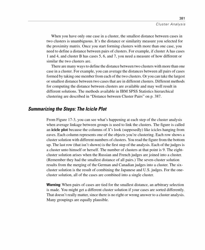
From Figure 17-3, you can see what’s happening at each step of the cluster analysis when average linkage between groups is used to link the clusters. The figure is called an icicle plot because the columns of X’s look (supposedly) like icicles hanging from eaves. Each column represents one of the objects you’re clustering. Each row shows a cluster solution with different numbers of clusters. You read the figure from the bottom up. The last row (that isn’t shown) is the first step of the analysis. Each of the judges is a cluster unto himself or herself. The number of clusters at that point is 9. The eight-cluster solution arises when the Russian and French judges are joined into a cluster. (Remember they had the smallest distance of all pairs.) The seven-cluster solution results from the merging of the German and Canadian judges into a cluster. The six-cluster solution is the result of combining the Japanese and U.S. judges. For the one-cluster solution, all of the cases are combined into a single cluster.

Warning: When pairs of cases are tied for the smallest distance, an arbitrary selection is made. You might get a different cluster solution if your cases are sorted differently. That doesn’t really matter, since there is no right or wrong answer to a cluster analysis. Many groupings are equally plausible.

382

Chapter 17

Figure 17-3Vertical icicle plot

Tip: If you have a large number of cases to cluster, you can make an icicle plot in which the cases are the rows. Specify Horizontal on the Cluster Plots dialog box.

Who’s in What Cluster?

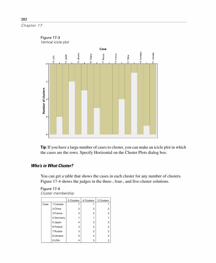
You can get a table that shows the cases in each cluster for any number of clusters. Figure 17-4 shows the judges in the three-, four-, and five-cluster solutions.

Figure 17-4Cluster membership

383

Cluster Analysis

Tip: To see how clusters differ on the variables used to create them, save the cluster membership number using the Save command and then use the Means procedure, specifying the variables used to form the clusters as the dependent variables and the cluster number as the grouping variable.

Tracking the Combinations: The Agglomeration Schedule

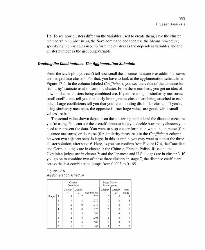
From the icicle plot, you can’t tell how small the distance measure is as additional cases are merged into clusters. For that, you have to look at the agglomeration schedule in Figure 17-5. In the column labeled Coefficients, you see the value of the distance (or similarity) statistic used to form the cluster. From these numbers, you get an idea of how unlike the clusters being combined are. If you are using dissimilarity measures, small coefficients tell you that fairly homogenous clusters are being attached to each other. Large coefficients tell you that you’re combining dissimilar clusters. If you’re using similarity measures, the opposite is true: large values are good, while small values are bad.

The actual value shown depends on the clustering method and the distance measure you’re using. You can use these coefficients to help you decide how many clusters you need to represent the data. You want to stop cluster formation when the increase (for distance measures) or decrease (for similarity measures) in the Coefficients column between two adjacent steps is large. In this example, you may want to stop at the three-cluster solution, after stage 6. Here, as you can confirm from Figure 17-4, the Canadian and German judges are in cluster 1; the Chinese, French, Polish, Russian, and Ukrainian judges are in cluster 2; and the Japanese and U.S. judges are in cluster 3. If you go on to combine two of these three clusters in stage 7, the distance coefficient across the last combination jumps from 0. 093 to 0.165.

Figure 17-5Agglomeration schedule

384

Chapter 17

The agglomeration schedule starts off using the case numbers that are displayed on the icicle plot. Once cases are added to clusters, the cluster number is always the lowest of the case numbers in the cluster. A cluster formed by merging cases 3 and 4 would forever be known as cluster 3, unless it happened to merge with cluster 1 or 2.

The columns labeled Stage Cluster First Appears tell you the step at which each of the two clusters that are being joined first appear. For example, at stage 4 when cluster 3 and cluster 6 are combined, you’re told that cluster 3 was first formed at stage 1 and cluster 6 is a single case and that the resulting cluster (known as 3) will see action again at stage 5. For a small dataset, you’re much better off looking at the icicle plot than trying to follow the step-by-step clustering summarized in the agglomeration schedule.

Tip: In most situations, all you want to look at in the agglomeration schedule is the coefficient at which clusters are combined. Look at the icicle plot to see what’s going on.

Plotting Cluster Distances: The Dendrogram

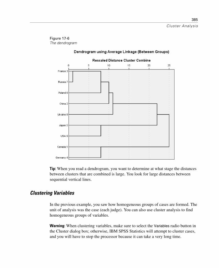
If you want a visual representation of the distance at which clusters are combined, you can look at a display called the dendrogram, shown in Figure 17-6. The dendrogram is read from left to right. Vertical lines show joined clusters. The position of the line on the scale indicates the distance at which clusters are joined. The observed distances are rescaled to fall into the range of 1 to 25, so you don’t see the actual distances; however, the ratio of the rescaled distances within the dendrogram is the same as the ratio of the original distances.

The first vertical line, corresponding to the smallest rescaled distance, is for the French and Russian alliance. The next vertical line is at the same distances for three merges. You see from Figure 17-5 that stages 2, 3, and 4 have the same coefficients. What you see in this plot is what you already know from the agglomeration schedule. In the last two steps, fairly dissimilar clusters are combined.

385

Cluster Analysis

Figure 17-6The dendrogram

Tip: When you read a dendrogram, you want to determine at what stage the distances between clusters that are combined is large. You look for large distances between sequential vertical lines.

Clustering Variables

In the previous example, you saw how homogeneous groups of cases are formed. The unit of analysis was the case (each judge). You can also use cluster analysis to find homogeneous groups of variables.

Warning: When clustering variables, make sure to select the Variables radio button in the Cluster dialog box; otherwise, IBM SPSS Statistics will attempt to cluster cases, and you will have to stop the processor because it can take a very long time.

386

Chapter 17

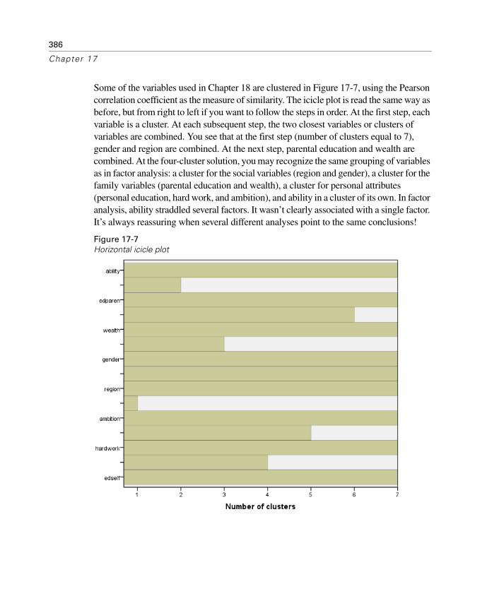
Some of the variables used in Chapter 18 are clustered in Figure 17-7, using the Pearson correlation coefficient as the measure of similarity. The icicle plot is read the same way as before, but from right to left if you want to follow the steps in order. At the first step, each variable is a cluster. At each subsequent step, the two closest variables or clusters of variables are combined. You see that at the first step (number of clusters equal to 7), gender and region are combined. At the next step, parental education and wealth are combined. At the four-cluster solution, you may recognize the same grouping of variables as in factor analysis: a cluster for the social variables (region and gender), a cluster for the family variables (parental education and wealth), a cluster for personal attributes (personal education, hard work, and ambition), and ability in a cluster of its own. In factor analysis, ability straddled several factors. It wasn’t clearly associated with a single factor. It’s always reassuring when several different analyses point to the same conclusions!

Figure 17-7Horizontal icicle plot

387

Cluster Analysis

Tip: When you use the correlation coefficient as a measure of similarity, you may want to take the absolute value of it before forming clusters. Variables with large negative correlation coefficients are just as closely related as variables with large positive coefficients.

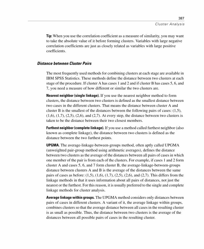
Distance between Cluster Pairs

The most frequently used methods for combining clusters at each stage are available in IBM SPSS Statistics. These methods define the distance between two clusters at each stage of the procedure. If cluster A has cases 1 and 2 and if cluster B has cases 5, 6, and 7, you need a measure of how different or similar the two clusters are.

Nearest neighbor (single linkage). If you use the nearest neighbor method to form clusters, the distance between two clusters is defined as the smallest distance between two cases in the different clusters. That means the distance between cluster A and cluster B is the smallest of the distances between the following pairs of cases: (1,5), (1,6), (1,7), (2,5), (2,6), and (2,7). At every step, the distance between two clusters is taken to be the distance between their two closest members.

Furthest neighbor (complete linkage). If you use a method called furthest neighbor (also known as complete linkage), the distance between two clusters is defined as the distance between the two furthest points.

UPGMA. The average-linkage-between-groups method, often aptly called UPGMA (unweighted pair-group method using arithmetic averages), defines the distance between two clusters as the average of the distances between all pairs of cases in which one member of the pair is from each of the clusters. For example, if cases 1 and 2 form cluster A and cases 5, 6, and 7 form cluster B, the average-linkage-between-groups distance between clusters A and B is the average of the distances between the same pairs of cases as before: (1,5), (1,6), (1,7), (2,5), (2,6), and (2,7). This differs from the linkage methods in that it uses information about all pairs of distances, not just the nearest or the furthest. For this reason, it is usually preferred to the single and complete linkage methods for cluster analysis.

Average linkage within groups. The UPGMA method considers only distances between pairs of cases in different clusters. A variant of it, the average linkage within groups, combines clusters so that the average distance between all cases in the resulting cluster is as small as possible. Thus, the distance between two clusters is the average of the distances between all possible pairs of cases in the resulting cluster.

388

Chapter 17

The methods discussed above can be used with any kind of similarity or distance measure between cases. The next three methods use squared Euclidean distances.

Ward’s method. For each cluster, the means for all variables are calculated. Then, for each case, the squared Euclidean distance to the cluster means is calculated. These distances are summed for all of the cases. At each step, the two clusters that merge are those that result in the smallest increase in the overall sum of the squared within-cluster distances. The coefficient in the agglomeration schedule is the within-cluster sum of squares at that step, not the distance at which clusters are joined.

Centroid method. This method calculates the distance between two clusters as the sum of distances between cluster means for all of the variables. In the centroid method, the centroid of a merged cluster is a weighted combination of the centroids of the two individual clusters, where the weights are proportional to the sizes of the clusters. One disadvantage of the centroid method is that the distance at which clusters are combined can actually decrease from one step to the next. This is an undesirable property because clusters merged at later stages are more dissimilar than those merged at early stages.

Median method. With this method, the two clusters being combined are weighted equally in the computation of the centroid, regardless of the number of cases in each. This allows small groups to have an equal effect on the characterization of larger clusters into which they are merged.

Tip: Different combinations of distance measures and linkage methods are best for clusters of particular shapes. For example, nearest neighbor works well for elongated clusters with unequal variances and unequal sample sizes.

K-Means Clustering

Hierarchical clustering requires a distance or similarity matrix between all pairs of cases. That’s a humongous matrix if you have tens of thousands of cases trapped in your data file. Even today’s computers will take pause, as will you, waiting for results.

A clustering method that doesn’t require computation of all possible distances is k-means clustering. It differs from hierarchical clustering in several ways. You have to know in advance the number of clusters you want. You can’t get solutions for a range of cluster numbers unless you rerun the analysis for each different number of clusters. The algorithm repeatedly reassigns cases to clusters, so the same case can move from cluster to cluster during the analysis. In agglomerative hierarchical clustering, on the other hand, cases are added only to existing clusters. They’re forever captive in their cluster, with a widening circle of neighbors.

389

Cluster Analysis

The algorithm is called k-means, where k is the number of clusters you want, since a case is assigned to the cluster for which its distance to the cluster mean is the smallest. The action in the algorithm centers around finding the k-means. You start out with an initial set of means and classify cases based on their distances to the centers. Next, you compute the cluster means again, using the cases that are assigned to the cluster; then, you reclassify all cases based on the new set of means. You keep repeating this step until cluster means don’t change much between successive steps. Finally, you calculate the means of the clusters once again and assign the cases to their permanent clusters.

Roman Pottery: The Example

When you are studying old objects in hopes of determining their historical origins, you look for similarities and differences between the objects in as many dimensions as possible. If the objects are intact, you can compare styles, colors, and other easily visible characteristics. You can also use sophisticated devices such as high-energy beam lines or spectrophotometers to study the chemical composition of the materials from which they are made. Hand et al. (1994) reports data on the percentage of oxides of five metals for 26 samples of Romano-British pottery described by Tubb et al. (1980). The five metals are aluminum (Al), iron (Fe), magnesium (Mg), calcium (Ca), and sodium (Na). In this section, you’ll study whether the samples form distinct clusters and whether these clusters correspond to areas where the pottery was excavated.

Before You Start

Whenever you use a statistical procedure that calculates distances, you have to worry about the impact of the different units in which variables are measured. Variables that have large values will have a large impact on the distance compared to variables that have smaller values. In this example, the average percentages of the oxides differ quite a bit, so it’s a good idea to standardize the variables to a mean of 0 and a standard deviation of 1. (Standardized variables are used in the example.) You also have to specify the number of clusters (k) that you want produced.

Tip: If you have a large data file, you can take a random sample of the data and try to determine a good number, or range of numbers, for a cluster solution based on the hierarchical clustering procedure. You can also use hierarchical cluster analysis to estimate starting values for the k-means algorithm.

390

Chapter 17

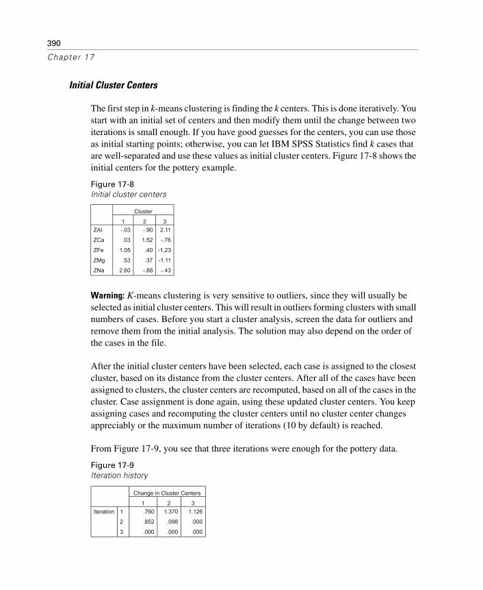
Initial Cluster Centers

The first step in k-means clustering is finding the k centers. This is done iteratively. You start with an initial set of centers and then modify them until the change between two iterations is small enough. If you have good guesses for the centers, you can use those as initial starting points; otherwise, you can let IBM SPSS Statistics find k cases that are well-separated and use these values as initial cluster centers. Figure 17-8 shows the initial centers for the pottery example.

Figure 17-8Initial cluster centers

Warning: K-means clustering is very sensitive to outliers, since they will usually be selected as initial cluster centers. This will result in outliers forming clusters with small numbers of cases. Before you start a cluster analysis, screen the data for outliers and remove them from the initial analysis. The solution may also depend on the order of the cases in the file.

After the initial cluster centers have been selected, each case is assigned to the closest cluster, based on its distance from the cluster centers. After all of the cases have been assigned to clusters, the cluster centers are recomputed, based on all of the cases in the cluster. Case assignment is done again, using these updated cluster centers. You keep assigning cases and recomputing the cluster centers until no cluster center changes appreciably or the maximum number of iterations (10 by default) is reached.

From Figure 17-9, you see that three iterations were enough for the pottery data.

Figure 17-9Iteration history

391

Cluster Analysis

Tip: You can update the cluster centers after each case is classified, instead of after all cases are classified, if you select the Use Running Means check box in the Iterate dialog box.

Final Cluster Centers

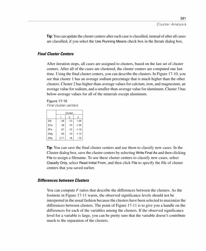
After iteration stops, all cases are assigned to clusters, based on the last set of cluster centers. After all of the cases are clustered, the cluster centers are computed one last time. Using the final cluster centers, you can describe the clusters. In Figure 17-10, you see that cluster 1 has an average sodium percentage that is much higher than the other clusters. Cluster 2 has higher-than-average values for calcium, iron, and magnesium, an average value for sodium, and a smaller-than-average value for aluminum. Cluster 3 has below-average values for all of the minerals except aluminum.

Figure 17-10Final cluster centers

Tip: You can save the final cluster centers and use them to classify new cases. In the Cluster dialog box, save the cluster centers by selecting Write Final As and then clicking File to assign a filename. To use these cluster centers to classify new cases, select Classify Only, select Read Initial From, and then click File to specify the file of cluster centers that you saved earlier.

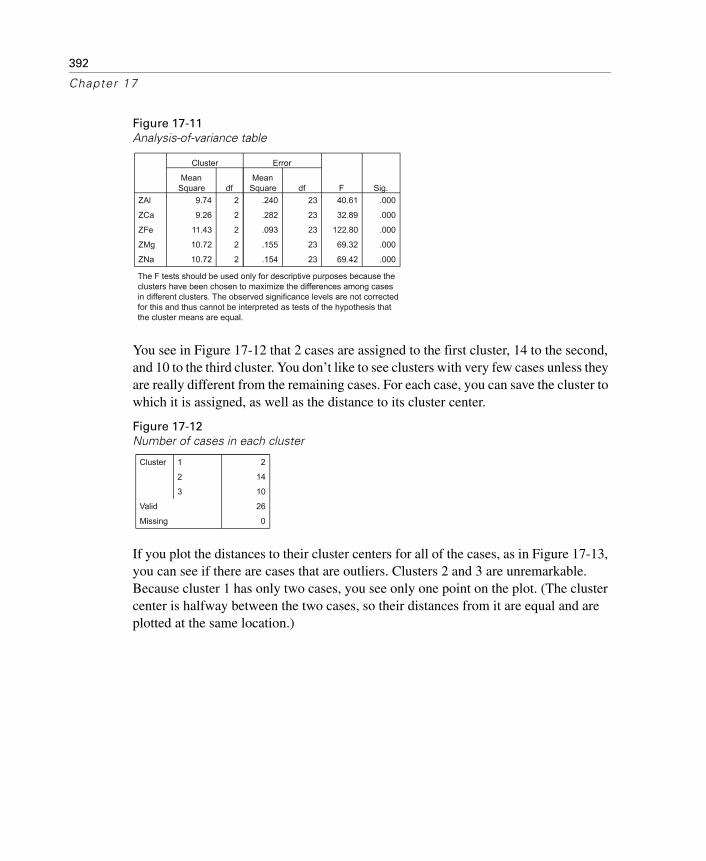
Differences between Clusters

You can compute F ratios that describe the differences between the clusters. As the footnote in Figure 17-11 warns, the observed significance levels should not be interpreted in the usual fashion because the clusters have been selected to maximize the differences between clusters. The point of Figure 17-11 is to give you a handle on the differences for each of the variables among the clusters. If the observed significance level for a variable is large, you can be pretty sure that the variable doesn’t contribute much to the separation of the clusters.

392

Chapter 17

Figure 17-11Analysis-of-variance table

You see in Figure 17-12 that 2 cases are assigned to the first cluster, 14 to the second, and 10 to the third cluster. You don’t like to see clusters with very few cases unless they are really different from the remaining cases. For each case, you can save the cluster to which it is assigned, as well as the distance to its cluster center.

Figure 17-12Number of cases in each cluster

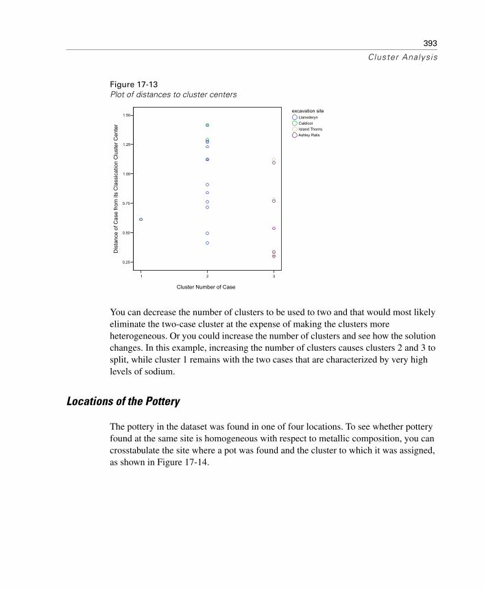
If you plot the distances to their cluster centers for all of the cases, as in Figure 17-13, you can see if there are cases that are outliers. Clusters 2 and 3 are unremarkable. Because cluster 1 has only two cases, you see only one point on the plot. (The cluster center is halfway between the two cases, so their distances from it are equal and are plotted at the same location.)

393

Cluster Analysis

Figure 17-13Plot of distances to cluster centers

You can decrease the number of clusters to be used to two and that would most likely eliminate the two-case cluster at the expense of making the clusters more heterogeneous. Or you could increase the number of clusters and see how the solution changes. In this example, increasing the number of clusters causes clusters 2 and 3 to split, while cluster 1 remains with the two cases that are characterized by very high levels of sodium.

Locations of the Pottery

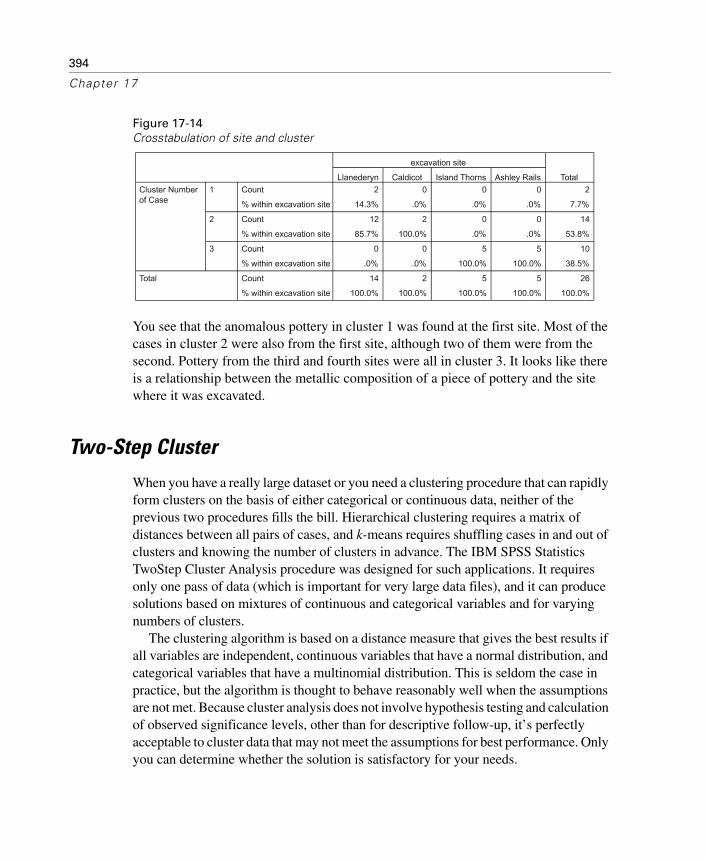
The pottery in the dataset was found in one of four locations. To see whether pottery found at the same site is homogeneous with respect to metallic composition, you can crosstabulate the site where a pot was found and the cluster to which it was assigned, as shown in Figure 17-14.

1 2 3

0.25

0.50

0.75

1.00

1.25

1.50excavation site

LlanederynCaldicotIsland ThornsAshley Rails

Cluster Number of Case

Dis

tanc

e of

Cas

e fro

m it

s C

lass

icat

ion

Clu

ster

Cen

ter

394

Chapter 17

Figure 17-14Crosstabulation of site and cluster

You see that the anomalous pottery in cluster 1 was found at the first site. Most of the cases in cluster 2 were also from the first site, although two of them were from the second. Pottery from the third and fourth sites were all in cluster 3. It looks like there is a relationship between the metallic composition of a piece of pottery and the site where it was excavated.

Two-Step Cluster

When you have a really large dataset or you need a clustering procedure that can rapidly form clusters on the basis of either categorical or continuous data, neither of the previous two procedures fills the bill. Hierarchical clustering requires a matrix of distances between all pairs of cases, and k-means requires shuffling cases in and out of clusters and knowing the number of clusters in advance. The IBM SPSS Statistics TwoStep Cluster Analysis procedure was designed for such applications. It requires only one pass of data (which is important for very large data files), and it can produce solutions based on mixtures of continuous and categorical variables and for varying numbers of clusters.

The clustering algorithm is based on a distance measure that gives the best results if all variables are independent, continuous variables that have a normal distribution, and categorical variables that have a multinomial distribution. This is seldom the case in practice, but the algorithm is thought to behave reasonably well when the assumptions are not met. Because cluster analysis does not involve hypothesis testing and calculation of observed significance levels, other than for descriptive follow-up, it’s perfectly acceptable to cluster data that may not meet the assumptions for best performance. Only you can determine whether the solution is satisfactory for your needs.

395

Cluster Analysis

Warning: The final solution may depend on the order of the cases in the file. To minimize the effect, arrange the cases in random order. Sort them by the last digit of their ID numbers or something similar.

Step 1: Preclustering: Making Little Clusters

The first step of the two-step procedure is formation of preclusters. The goal of preclustering is to reduce the size of the matrix that contains distances between all possible pairs of cases. Preclusters are just clusters of the original cases that are used in place of the raw data in the hierarchical clustering. As a case is read, the algorithm decides, based on a distance measure, if the current case should be merged with a previously formed precluster or start a new precluster. When preclustering is complete, all cases in the same precluster are treated as a single entity. The size of the distance matrix is no longer dependent on the number of cases but on the number of preclusters.

Step 2: Hierarchical Clustering of Preclusters

In the second step, IBM SPSS Statistics uses the standard hierarchical clustering algorithm on the preclusters. Forming clusters hierarchically lets you explore a range of solutions with different numbers of clusters.

Tip: The Options dialog box lets you control the number of preclusters. Large numbers of preclusters give better results because the cases are more similar in a precluster; however, forming many preclusters slows the algorithm.

Clustering Newspaper Readers: The Example

As an example of two-step clustering, you’ll consider the General Social Survey data described in Chapter 6. Both categorical and continuous variables are used to form the clusters. The categorical variables are sex, frequency of reading a newspaper, and highest degree. The continuous variable is age.

Some of the options you can specify when using two-step clustering are:

Standardization: The algorithm will automatically standardize all of the variables unless you override this option.

396

Chapter 17

Distance measures: If your data are a mixture of continuous and categorical variables, you can use only the log-likelihood criterion. The distance between two clusters depends on the decrease in the log-likelihood when they are combined into a single cluster. If the data are only continuous variables, you can also use the Euclidean distance between two cluster centers. Depending on the distance measure selected, cases are assigned to the cluster that leads to the largest log-likelihood or to the cluster that has the smallest Euclidean distance.

Number of clusters: You can specify the number of clusters to be formed, or you can let the algorithm select the optimal number based on either the Schwarz Bayesian Criterion or the Akaike information criterion.

Outlier handling: You have the option to create a separate cluster for cases that don’t fit well into any other cluster.

Range of solutions: You can specify the range of cluster solutions that you want to see.

Tip: If you’re planning to use this procedure, consult the algorithms documentation in the Help system for additional details.

Examining the Number of Clusters

Once you make some choices or do nothing and go with the defaults, the clusters are formed. At this point, you can consider whether the number of clusters is “good.” If you use automated cluster selection, IBM SPSS Statistics finds the number of clusters at which the Schwarz Bayesian Criterion, abbreviated BIC (the I stands for Information), becomes small and the change in BIC between adjacent number of clusters is small. For this example, the algorithm selects three clusters.

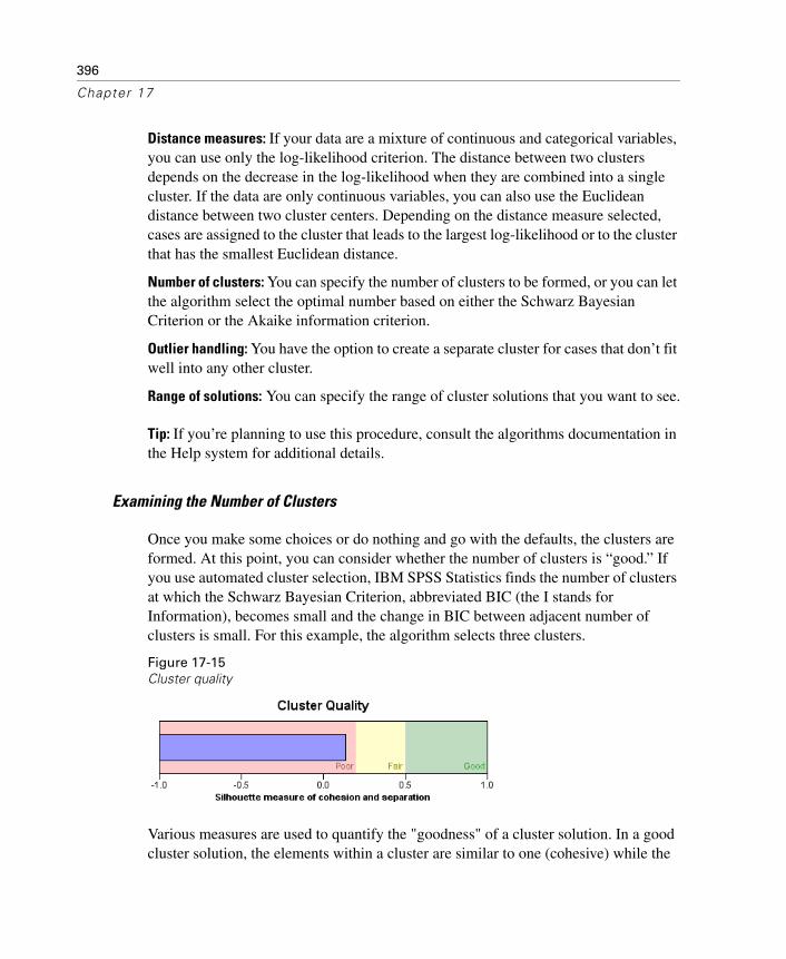
Figure 17-15Cluster quality

Various measures are used to quantify the "goodness" of a cluster solution. In a good cluster solution, the elements within a cluster are similar to one (cohesive) while the

397

Cluster Analysis

clusters themselves are quite different (separated). A popular measure is the silhouette coefficient, which is a measure of both cohesion and separation. For each element in a cluster, you calculate the average distance to all other elements in its cluster and the average distance to all elements in each of the other clusters. For each element, the silhouette measure is the difference between the smallest average between cluster distance and the average within cluster distance, divided by the larger of the two distances. In a good solution, the within-cluster distances are small and the between-cluster distances are large, resulting in a silhouette measure close to the maximum value of 1. If the silhouette measure is negative, the average distance of a case to members of its own cluster is larger than the average distance to cases in other clusters, an undesirable feature. The silhouette measure for a cluster is just the average of the silhouette measures for the cases within the cluster. The silhouette measure ranges from –1 to +1. In this example, from Figure 17-15, you see that the silhouette measure is close to 0, indicating that the cluster solution is far from stellar. We'll still soldier on.

In Figure 17-16, you see the distribution of cases in the final cluster solution. (Positioning the cursor over a pie slice shows you the number of cases in the cluster.) The largest cluster has 44% of the cases and the smallest has 27%. In most applications, you do not want many small clusters but instead prefer a solution with a small number of larger clusters.

398

Chapter 17

Figure 17-16Distribution of cases in clusters

Warning: When you have cases that are very different from other cases and not necessarily similar to each other, they can have a large impact on cluster formation by increasing the overall number of clusters or making clusters less homogeneous. One solution to the problem is to create an outlier cluster that contains all cases that do not fit well with the rest. IBM SPSS Statistics will do this automatically for you if you select Outlier Treatment in the Options dialog box.

Examining the Importance of Features

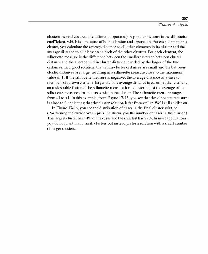
IBM SPSS Statistics offers numerous displays to help you understand what types of objects are in each of the clusters and the importance of each of the features/variables in cluster formation. Figure 17-17 summarizes the characteristics of each cluster. The

399

Cluster Analysis

features are arranged in descending order of importance for cluster formation. For categorical variables, the percentage of cases in each of the modal categories is shown; for scale variables, the average value is given. By default, the clusters are arranged in descending sizes.

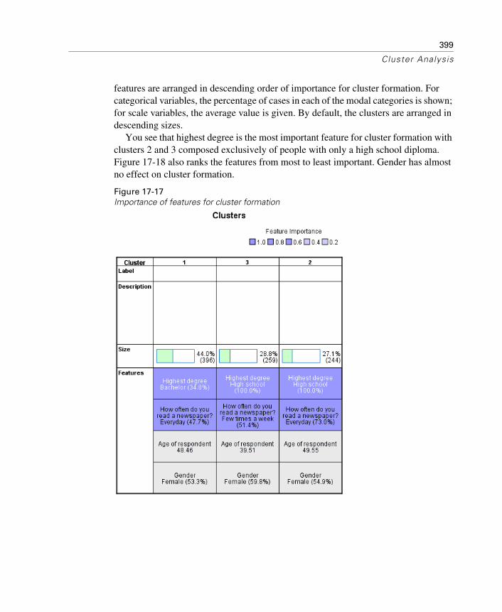
You see that highest degree is the most important feature for cluster formation with clusters 2 and 3 composed exclusively of people with only a high school diploma. Figure 17-18 also ranks the features from most to least important. Gender has almost no effect on cluster formation.

Figure 17-17Importance of features for cluster formation

400

Chapter 17

Figure 17-18Feature importance

Examining the Composition of Individual Clusters

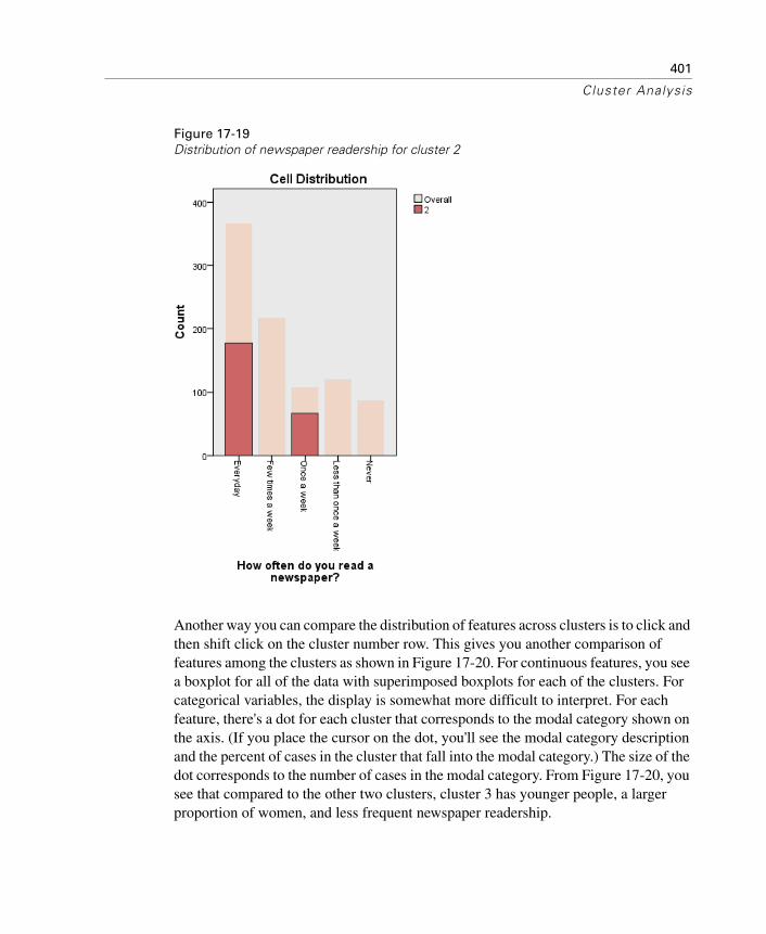
You can click on the feature/cluster cell of interest for more detailed information about the distribution of a feature within a cluster. For categorical variables, a bar chart is shown in the right pane of the model viewer; for continuous variables, a histogram. For example, Figure 17-19 is the cell information for newspaper readership for cluster 2, compared to the overall distribution.

401

Cluster Analysis

Figure 17-19Distribution of newspaper readership for cluster 2

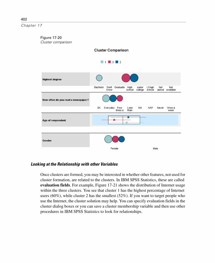
Another way you can compare the distribution of features across clusters is to click and then shift click on the cluster number row. This gives you another comparison of features among the clusters as shown in Figure 17-20. For continuous features, you see a boxplot for all of the data with superimposed boxplots for each of the clusters. For categorical variables, the display is somewhat more difficult to interpret. For each feature, there's a dot for each cluster that corresponds to the modal category shown on the axis. (If you place the cursor on the dot, you'll see the modal category description and the percent of cases in the cluster that fall into the modal category.) The size of the dot corresponds to the number of cases in the modal category. From Figure 17-20, you see that compared to the other two clusters, cluster 3 has younger people, a larger proportion of women, and less frequent newspaper readership.

402

Chapter 17

Figure 17-20Cluster comparison

Looking at the Relationship with other Variables

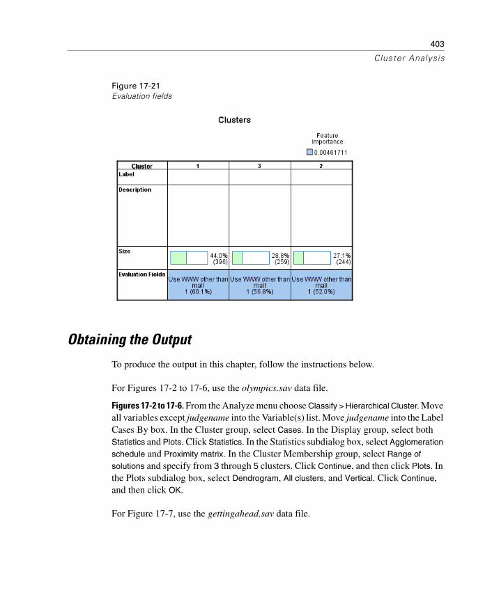
Once clusters are formed, you may be interested in whether other features, not used for cluster formation, are related to the clusters. In IBM SPSS Statistics, these are called evaluation fields. For example, Figure 17-21 shows the distribution of Internet usage within the three clusters. You see that cluster 1 has the highest percentage of Internet users (60%), while cluster 2 has the smallest (52%). If you want to target people who use the Internet, the cluster solution may help. You can specify evaluation fields in the cluster dialog boxes or you can save a cluster membership variable and then use other procedures in IBM SPSS Statistics to look for relationships.

403

Cluster Analysis

Figure 17-21Evaluation fields

Obtaining the Output

To produce the output in this chapter, follow the instructions below.

For Figures 17-2 to 17-6, use the olympics.sav data file.

Figures 17-2 to 17-6. From the Analyze menu choose Classify > Hierarchical Cluster. Move all variables except judgename into the Variable(s) list. Move judgename into the Label Cases By box. In the Cluster group, select Cases. In the Display group, select both Statistics and Plots. Click Statistics. In the Statistics subdialog box, select Agglomeration schedule and Proximity matrix. In the Cluster Membership group, select Range of

solutions and specify from 3 through 5 clusters. Click Continue, and then click Plots. In the Plots subdialog box, select Dendrogram, All clusters, and Vertical. Click Continue, and then click OK.

For Figure 17-7, use the gettingahead.sav data file.

404

Chapter 17

Figure 17-7. From the Analyze menu choose Classify > Hierarchical Cluster. Move ability, ambition, edparen, edself, hardwork, gender, region, and wealth into the Variable(s) list. In the Cluster group, select Variables. Select both Statistics and Plots in the Display group. Click Plots. In the Plots subdialog box, select All clusters in the Icicle group and Horizontal in the Orientation group. Click Continue and then click Method. In the Method subdialog box, select Interval in the Measure group, and select Pearson

correlation as Interval measure. Click Continue, and then click OK.

For Figures 17-8 to 17-14, use the pottery.sav data file.

Figures 17-8 to 17-12. From the Analyze menu choose Classify > K-Means Cluster. Move ZAl, ZCa, ZFe, ZMg, and ZNa into the Variables list, and specify 3 as Number of Clusters. Click Options and in the K-Means Cluster Analysis Options subdialog box, select both Initial cluster centers and ANOVA table. Click Continue, and then click Save. Select both Cluster membership and Distance from cluster center. Click Continue, and then click OK.

Figure 17-13. From the Graphs menu, choose Chart Builder. From the gallery, select Scatter/Dot, then double-click the Simple Scatter icon. Drag QCL_1 to the X-Axis drop box and QCL_2 to the Y-Axis drop box.

Figure 17-14. From the Analyze menu choose Descriptive Statistics > Crosstabs. Move QCL_1 into the Row(s) list and site into the Column(s) list. Click Cells, and in the Crosstabs Cell Display subdialog box, select Observed in the Counts group and Column in the Percentages group. Click Continue, and then click OK.

For Figures 17-15 to 17-21, use the gssdata.sav data file.

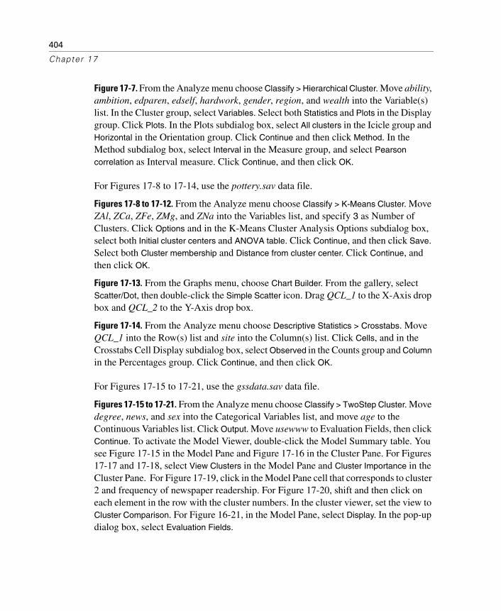
Figures 17-15 to 17-21. From the Analyze menu choose Classify > TwoStep Cluster. Move degree, news, and sex into the Categorical Variables list, and move age to the Continuous Variables list. Click Output. Move usewww to Evaluation Fields, then click Continue. To activate the Model Viewer, double-click the Model Summary table. You see Figure 17-15 in the Model Pane and Figure 17-16 in the Cluster Pane. For Figures 17-17 and 17-18, select View Clusters in the Model Pane and Cluster Importance in the Cluster Pane. For Figure 17-19, click in the Model Pane cell that corresponds to cluster 2 and frequency of newspaper readership. For Figure 17-20, shift and then click on each element in the row with the cluster numbers. In the cluster viewer, set the view to Cluster Comparison. For Figure 16-21, in the Model Pane, select Display. In the pop-up dialog box, select Evaluation Fields.