ICES REPORT 12-13

April 2012

Solid T-spline Construction from BoundaryTriangulations with Arbitrary Genus Topology

by

Wenyan Wang, Yongjie Zhang, Lei Liu and Thomas J.R. Hughes

The Institute for Computational Engineering and SciencesThe University of Texas at AustinAustin, Texas 78712

Reference: Wenyan Wang, Yongjie Zhang, Lei Liu and Thomas J.R. Hughes, Solid T-spline Construction fromBoundary Triangulations with Arbitrary Genus Topology, ICES REPORT 12-13, The Institute for ComputationalEngineering and Sciences, The University of Texas at Austin, April 2012.

Report Documentation Page Form ApprovedOMB No. 0704-0188

Public reporting burden for the collection of information is estimated to average 1 hour per response, including the time for reviewing instructions, searching existing data sources, gathering andmaintaining the data needed, and completing and reviewing the collection of information. Send comments regarding this burden estimate or any other aspect of this collection of information,including suggestions for reducing this burden, to Washington Headquarters Services, Directorate for Information Operations and Reports, 1215 Jefferson Davis Highway, Suite 1204, ArlingtonVA 22202-4302. Respondents should be aware that notwithstanding any other provision of law, no person shall be subject to a penalty for failing to comply with a collection of information if itdoes not display a currently valid OMB control number.

1. REPORT DATE APR 2012 2. REPORT TYPE

3. DATES COVERED 00-00-2012 to 00-00-2012

4. TITLE AND SUBTITLE Solid T-spline Construction from Boundary Triangulations withArbitrary Genus Topology

5a. CONTRACT NUMBER

5b. GRANT NUMBER

5c. PROGRAM ELEMENT NUMBER

6. AUTHOR(S) 5d. PROJECT NUMBER

5e. TASK NUMBER

5f. WORK UNIT NUMBER

7. PERFORMING ORGANIZATION NAME(S) AND ADDRESS(ES) University of Texas at Austin,Institute for Computational Engineeringand Sciences,Austin,TX,78712

8. PERFORMING ORGANIZATIONREPORT NUMBER

9. SPONSORING/MONITORING AGENCY NAME(S) AND ADDRESS(ES) 10. SPONSOR/MONITOR’S ACRONYM(S)

11. SPONSOR/MONITOR’S REPORT NUMBER(S)

12. DISTRIBUTION/AVAILABILITY STATEMENT Approved for public release; distribution unlimited

13. SUPPLEMENTARY NOTES

14. ABSTRACT A comprehensive scheme is described to construct rational solid T-splines from boundary triangulationswith arbitrary topology. To extract the topology of the input geometry, we first compute a smoothharmonic scalar field defined over the mesh and saddle points are extracted to determine the topology. Bydealing with the saddle points, a polycube whose topology is equivalent to the input geometry is built and itserves as the parametric domain for the solid T-spline. A polycube mapping is then used to build aone-to-one correspondence between the input triangulation and the polycube boundary. After that, wechoose the deformed octree subdivision of the polycube as the initial T-mesh, and make it valid throughpillowing, quality improvement and applying templates to handle extraordinary nodes and partialextraordinary nodes. The obtained T-spline is C2-continuous everywhere over the boundary surface exceptfor the local region surrounding polycube corner nodes. The e ciency and robustness of the presentedtechnique are demonstrated with several applications in isogeometric analysis.

15. SUBJECT TERMS

16. SECURITY CLASSIFICATION OF: 17. LIMITATION OF ABSTRACT Same as

Report (SAR)

18. NUMBEROF PAGES

13

19a. NAME OFRESPONSIBLE PERSON

a. REPORT unclassified

b. ABSTRACT unclassified

c. THIS PAGE unclassified

Standard Form 298 (Rev. 8-98) Prescribed by ANSI Std Z39-18

Solid T-spline Construction from Boundary Triangulations with ArbitraryGenus Topology

Wenyan Wang a, Yongjie Zhang a,∗, Lei Liu a, and Thomas J.R. Hughes baDepartment of Mechanical Engineering, Carnegie Mellon University

Pittsburgh, PA 15213, USAbInstitute for Computational Engineering and Sciences, The University of Texas at Austin

Austin, TX 78712, USA

Abstract

A comprehensive scheme is described to construct rational solid T-splines from boundary triangulations with arbitrary topology. To extractthe topology of the input geometry, we first compute a smooth harmonic scalar field defined over the mesh and saddle points are extracted todetermine the topology. By dealing with the saddle points, a polycube whose topology is equivalent to the input geometry is built and it servesas the parametric domain for the solid T-spline. A polycube mapping is then used to build a one-to-one correspondence between the inputtriangulation and the polycube boundary. After that, we choose the deformed octree subdivision of the polycube as the initial T-mesh, andmake it valid through pillowing, quality improvement and applying templates to handle extraordinary nodes and partial extraordinary nodes.The obtained T-spline is C2-continuous everywhere over the boundary surface except for the local region surrounding polycube corner nodes.The efficiency and robustness of the presented technique are demonstrated with several applications in isogeometric analysis.

Key words: Solid T-spline Construction, Arbitrary Genus Topology, Polycube, Rational T-spline, Isogeometric Analysis

1. Introduction

For tight integration of Design-Through-Analysis, isogeo-metric analysis [11] was proposed which utilizes spline func-tions as a basis. The current state-of-the-art in engineering de-sign and analysis is built on disparate geometric foundations.Spline representation is popular in design while polygonal meshrepresentation is generally used in analysis. This leads to manytranslational difficulties which affect the efficiency and accuracyof the entire process. Isogeometric analysis utilizes the same ba-sis functions as the geometry representation, and consequently,analysis can be carried out over an exact spline representa-tion of the geometry. Similar to other physically-based anal-ysis, solid models, which can represent both boundary shapeand interior volume, are required for many applications in iso-geometric analysis. A fundamental step for the unified Design-Through-Analysis technologies is to automatically constructsolid trivariate spline models from boundary representations.

The advent of T-splines [16] gives more flexibility for ge-ometric modeling, allowing local refinement, non-rectangulardomains in 2D and non-cubic domains in 3D. T-splines can

∗ Corresponding author: Y. Zhang. Tel: (412) 268-5332; Fax: (412) 268-3348; E-mail address: jessicaz@andrew.cmu.edu.

represent a complicated design with complex topology as a sin-gle watertight geometry, avoiding splitting the model into sev-eral patches. T-splines are a superior alternative to and also arecompatible with NURBS, which is the current geometry stan-dard in CAD systems. The flexibility of T-splines makes theman ideal discretization technology for isogeometric analysis.

Several methods have been developed recently to con-struct solid T-splines. A solid T-spline generation method wasdescribed for genus-zero geometries [4]. In [13], trivariateT-splines were defined based on the generalized polycubeparametrization. Another spline scheme based on polycubes,called restricted trivariate polycube splines, was developedin [21]. This algorithm is based on semi-standard T-splines.It requires calculation of weights and the obtained T-splineelements are uniform. For all these methods, the polycube isgenerated manually for a given geometry. In addition, the con-structed T-spline model may contain some negative Jacobianelements, which is unsuitable for analysis.

In our earlier work, we developed a mapping-based ratio-nal solid T-spline construction method for genus-zero geom-etry from the boundary surface triangulation [23]. To extendthis algorithm to more general geometry, we first extract thetopology of the input geometry and build a polycube which ap-proximates the input geometry, by computing a harmonic field

Preprint submitted to Elsevier 2 April 2012

and dealing with its critical points. Due to its regular structure,the polycube is suitable for serving as the parametric domainof the tensor-product spline representations. Here, a trivariatesolid T-spline is built upon the generated polycube. We thenbuild a parametric mapping between the triangulation and theboundary of the polycube. In the following steps, an octree sub-division is applied to the polycube and the initial T-mesh is adeformation of its subdivision. The subdivision continues untilthe surface approximation error is less than a given tolerance.After that, the valid T-mesh is obtained through pillowing, T-mesh quality improvement, and applying templates to handleextraordinary nodes and partial extraordinary nodes. Finally,Bezier elements are extracted with all positive Jacobians, andthey are suitable for isogeometric analysis.

Compared with other existing methods, our solid T-splineconstruction scheme has several attractive properties: (1) it canbe used for arbitrary topology and the polycube is created au-tomatically; (2) the obtained trivariate T-spline has a one-piecerepresentation and it contains very few irregular nodes wherethe continuity degenerates; (3) it employs rational T-spline ba-sis, which guarantee partition of unity by definition; (4) it pro-duces high quality analysis-suitable T-spline elements with allpositive Jacobians; and (5) with an adaptive refinement scheme,the resulting T-spline model is an efficient representation foranalysis.

The remainder of this paper is organized as follows. Section2 reviews related work. Section 3 presents an overview of theconstruction algorithm. The polycube construction algorithmis presented in Section 4. The T-mesh construction algorithmfrom the polycube is described in Section 5 and solid T-splineconstruction is presented in Section 6. Section 7 presents ex-amples and Section 8 draws conclusions.

2. Previous Work

Harmonic Fields. A harmonic field is the solution to theLaplace equation with given boundary conditions and it definesa scalar or vector field over the domain. For a given mesh, har-monic fields can be computed by solving a linear system of alge-braic equations with imposed boundary conditions. Harmonicfields have certain desirable properties, such as smoothness,and are free of extraneous critical points. Due to these proper-ties, harmonic fields have been shown to provide effective toolfor a number of geometry processing problems. Dong et al. [3]traced the integral lines through the gradient and orthogonalvector fields of a harmonic field for quadrilateral remeshing ofarbitrary manifolds. Based on a harmonic map, a 3D geomet-ric metamorphosis method was developed for any two objectswhich are topologically equivalent to a sphere or a disk [12].Joshi et al. [19] utilized harmonic coordinates, which are gen-eralized barycentric coordinates, in volume deformation.

Surface Parameterization. A surface parameterization is aone-to-one mapping from one surface in 3D to a suitable planardomain. Parameterization is a powerful tool and necessary formany geometry processing tasks, including data fitting, texturemapping, and remeshing. Many significant advances have beenmade for surface parameterization [5, 6, 18]. In [8], a conformal

mapping method was presented to map a genus-zero closedsurface onto the unit sphere by minimizing the harmonic energyof the map. For parameterization of an arbitrary genus objectto simpler surfaces of the same genus, the mesh is usuallyfirst segmented into disk-like patches and then each patch ismapped onto the corresponding plane. In [7], Gu et al. solvedthe problem of global conformal parameterization for surfacesof arbitrary topology, with or without boundaries.

Polycube Generation and Application. A polyube is a solidcomposed of cubes. It can be used to very roughly approxi-mate the geometry of a 3D object while faithfully replicating itstopology. Due to its highly regular structure, the polycube canbe used as the parametric domain for surface parameterizationand spline modeling. However, in practice due to the complexityof shapes, polycubes are usually constructed manually, entail-ing considerable effort. In order to produce polycubes with lessuser intervention, He et al. [9] developed a method to constructa 3D polycube by extruding the axis-aligned polygons whichapproximate the horizontal curved intersection contours. Basedon the polycube, a global parameterization technique, polycubemap [19], was first used for seamless texture mapping. Wanget al. developed a technique to build the polycube splines uponthe polycube map for surface modeling [20]. In [13], an algo-rithm was developed to construct trivariate T-splines over gen-eralized polycubes with a global “one-piece” representation forgeneral volumetric data. In [21], a theoretical volumetric mod-eling framework was presented to construct restricted trivariatepolycube splines, in which the blending functions are strictlybounded within the solid polycube domain.

Solid Spline Modeling. Only a few works have been de-voted to solid spline modeling. In [10], a trivariate simplexspline modeling method was developed based on a tetrahedraldecomposition of any 3D domain with complicated geometryand arbitrary topology. In [24], a skeleton-based method wasdeveloped to construct solid NURBS for isogeometric analysisof arterial blood flow. A method was presented in [1] to gener-ate NURBS parameterizations of swept volumes by sweeping aclosed curve, and isogeometric analysis was applied to the gen-erated NURBS model. Based on discrete harmonic functions,a volumetric parameterization was used to construct a singletrivariate B-spline [14]. By using adaptive tetrahedral meshingand a mesh untangling technique, an algorithm was developedto construct a trivariate T-spline representation of genus-zerosolids [4].

It is still a challenging problem to automatically create poly-cubes for high genus geometry and use them in constructinganalysis-suitable trivariate T-splines. In this paper, we utilize aharmonic field defined over the input mesh to build the polycubeautomatically, and then construct the rational solid T-spline overthe polycube. We include pillowing and quality improvementtechniques to guarantee that the obtained solid T-spline can beused for analysis directly.

3. Algorithm Overview

As shown in Figure 1, there are three main stages for con-structing a solid T-spline from a given boundary triangle mesh

2

with arbitrary genus topology. From the input triangle mesh,we first compute a harmonic scalar field defined over the mesh,extract the geometry topology, and then generate the polycubewith the same topology. Adopting the polycube as the paramet-ric domain, we build the valid T-mesh in the second stage andconstruct solid T-splines in the last stage.

Fig. 1. An overview of the solid T-spline construction algorithm from thegiven boundary triangle mesh with arbitrary topology.

The polycube generation stage consists of two steps:(i) Harmonic Field Calculation - We build a smooth har-

monic scalar field defined over the input mesh. Based onthis field, we compute its gradient field and an orthogo-nal vector field;

(ii) Handing Critical Points - From the harmonic field, wedetermine all the critical points where the first partialderivatives vanish. These critical points include extremepoints and saddle points. We design different methods todeal with each type of point in order to build the polycube.The polycube edges are traced along the gradient andisocontour directions.

Based on the polycube, the T-mesh is constructed. Thereare four different kinds of nodes in the solid T-mesh: regularnodes, partial extraordinary nodes, extraordinary nodes and T-junctions. A regular node is a node around which the localT-mesh is a structured mesh, like node A in Figure 2(a). Bothpartial extraordinary nodes and extraordinary nodes are irreg-ular, and they can be distinguished using reflection edges. Re-flection edges are a pair of adjacent edges with one commonnode, and the set formed by all the elements sharing one edgeis topologically symmetric with the set of elements sharing theother. For example, AB and AC in Figure 2(b) are a pair ofreflection edges. A partial extraordinary node is an irregularnode about which some but not all of its adjacent edges havereflection edges, like node A in Figure 2(b). An extraordinarynode is an irregular node about which none of its adjacentedges has a reflection edge, such as node A in Figure 2(c). AT-junction terminates a row of control points in one or more

parametric directions, which may lie on an edge or a face. Insolid T-splines, an edge T-junction is a T-junction which lieson one edge, such as node M in Figure 2(d). A face T-junctionis a T-junction lying on one face, such as node P in Figure 2(e).

(a) (b)

(c) (d) (e)

Fig. 2. Four types of nodes in solid T-meshes. (a) Regular node; (b) partialextraordinary node; (c) extraordinary node; (d) edge T-junction; and (e) faceT-junction.

The T-mesh construction stage consists of four steps:(i) Parametric Mapping - We build a parametric mapping

between the input triangle mesh and the boundary of thegenerated polycube;

(ii) Octree Subdivision and Projection - An initial T-mesh isobtained by an octree subdivision of the polycube andeach node on the polycube boundary is projected ontothe boundary surface based on the mapping;

(iii) Pillowing and Quality Improvement - We insert one pil-lowed layer on the boundary and improve T-mesh qualityby smoothing and optimization;

(iv) Handling Extraordinary Nodes and Partial ExtraordinaryNodes - In order to obtain a gap-free T-mesh, we applytemplates to each extraordinary node and partial extraor-dinary node in the initial T-mesh.

In this stage, we use the polycube as the parametric domainfor the solid T-spline construction. In the octree subdivisionstep, we choose the existing T-junction parametric values tosubdivide each octree cell as much as possible, instead of al-ways using the central parametric value. Based on the valid T-mesh, the knot vectors for each node are determined by travers-ing T-mesh faces and edges [17], and the solid T-spline is con-structed based on the rational T-spline definition [22]. Bezierelements are extracted to serve as the primary computationalobjects in isogeometric analysis. See [2, 15] for elaboration.

4. Polycube Generation

In this section, we discuss the detailed algorithm of the poly-cube generation from the input boundary triangulation. Thepolycube must be constructed in a geometrically approximateand topologically equivalent way. To achieve this goal, we first

3

compute a harmonic function defined over the input mesh T ,derive two orthogonal fields from the harmonic function, andextract the topology structure of T by examining critical points.

4.1. Harmonic Field Calculation

To extract the topological structure of the input mesh T ⊂R3, we construct a harmonic function f : T →R, such that

4 f = 0 (1)

subject to the boundary condition that vertices in the predefinedset S min and S max have the minimum and maximum values. 4is the Laplace operator. S min and S max are either given by theuser, or they can also be determined by selecting the bottom-most and top-most points on T . Basically, computing such aharmonic function is to assign a scalar value to each vertex inT . For a triangle mesh, we use the discretization of the Laplaceoperator

4 fi =∑j∈Ni

wi j( f (V j)− f (Vi)) = 0, (2)

where Vi,V j ∈ T , wi j is the weight and Ni is the number ofvertices adjacent to Vi. Here, we choose the weights, wi j =

cotαi j +cotβi j, where αi j and βi j are the opposite angles of theedge Vi −V j. From the discretization of the Laplace operator,the scalar function f can be obtained by solving a linear system.Figure 3(a) shows the scalar function defined over the “Eight”model. The red region has the maximal scalar value and theblue region has the minimal scalar value.

From the scalar field f , we compute both the gradient g1 =∇ fand one orthogonal vector field g2 (the isocontour field). Due tothe properties of a harmonic scalar field, the obtained directionfields are guaranteed to be smooth and free of extraneous criticalpoints. For one triangle (Vi,V j,Vk), suppose−→n is the unit normalvector. The gradient vector g1 = ∇ f is obtained by solving thefollowing linear system [3]:

V j−Vi

Vk −V j

−→n

[g1

]=

f j− fi

fk − f j

0

. (3)

The field g2 is along the isocontour directions of f . Hence, forone scalar value, we simply find out its isocontour to obtainthe vector field g2 for the triangle mesh. Once we obtain thetwo orthogonal vector fields g1 and g2, we can trace alongthe flow lines. A flow line is a piecewise-linear curve definedover the mesh whose edges are along one of the vector fields.There are two cases for tracing the gradient flow, the regularcase and the edge case. As shown in Figures 3(b-c), vertex Ais the starting point, the green arrows represent the gradientdirection for each incident triangle, and we wish to trace theflow line from A by walking across the incident triangles alongthe gradient direction. For the regular case in (b), starting fromA we extend the gradient line by crossing one of its incidenttriangles. In this case, we add one new vertex B to advance theflow line. For the edge case in (c), the flow field converges on

an edge AB and we simply follow this edge. In Figures 3(b-c),the red edges are the newly obtained flow line segments. Thenext step is to consider vertex B and trace the flow line from itusing the same procedure.

(b)

(a) (c)

Fig. 3. (a) Harmonic scalar field with saddle points rendered in pink for the“Eight” model. (b-c) Two cases for tracing the gradient flow line from agiven vertex A. (b) Regular case; and (c) edge case.

In addition, based on the scalar field, we can then determineall the critical points of f , that is, those points whose partialderivatives vanish. These points include:– Minimal point - Points in set S min;– Maximal point - Points in set S max;– Splitting saddle point - Points where the geometry splits;– Merging saddle point - Points where the geometry merges.

(a) (b) (c) (d)

Fig. 4. Configurations around a regular (a), minimal (b), maximal (c), andsaddle point (d).

Figure 4 shows the configurations of a regular, minimal, max-imal and saddle point. The red points denote the vertices witha larger scalar value compared with the center point and theblue points denote the vertices with a smaller scalar value. Asshown in Figure 4(a), around one regular point, vertices on oneside all have a larger scalar value and vertices on the other sideall have a smaller scalar value. For a minimal/maximal point,all the vertices surrounding it have a larger or smaller scalarvalue. For a saddle point, the sign changes alternately along itscircumferential direction.

Discussion: The harmonic field is controlled by the user-defined minima and maxima constraints, it then affects the poly-cube generation and alignment of the solid T-spline. To ensure

4

(a) (b) (c) (d)

Fig. 5. (a-b) Handling the minimal level; and (c-d) handling one splitting saddle point S .

the harmonic field follows the geometric shape of the input sur-face, generally it is better to place these constraints on the tipsof the geometry and also consider symmetry. For example, inthe “Eight” model (Figure 3(a)), we assign the constraints atthe top and the bottom.

4.2. Handing Critical Points

We need to handle various critical points: minimal, maximal,splitting saddle and merging saddle points. We first computeall the scalar levels or isocontours at which there are criticalpoints. Let fi denote the isovalue of Li and Ci denote thecorresponding isocontour. For level Li with saddle points, twosets of isocontours, C−i and C+

i , are computed by using theisovalue fi with a small perturbation δ. For the minimal ormaximal level, only one isocontour is computed.

Suppose level Li contains one minimal point. At level Li,four seed points (Pl

i, j, j = 0, . . . ,3) are chosen for each closedcurve as shown in Figures 5(a-b), which correspond to the fourlower corners of the cube Ci with the unit parametric length.The parametric value of the other vertices lying on this isocon-tour will be computed using the chord-length parameterization.From these seed points Pl

i, j we trace the gradient flow line un-til it intersects with the isocontour C−i+1 of the next level Li+1at Pu

i, j (Li+1 may contain a saddle or maximal point). The redcurves in Figure 5 are traced gradient lines, and the black onesare isocontours. The four vertices Pu

i, j ( j = 0, . . . ,3) correspondto the four upper corners of Ci. The traced four curves are thenmapped onto the four vertical edges of the cube, and Pl

i, j andPu

i, j serve as the eight corners. Then the polycube constructionprocess advances to the next level.

For level Li with a splitting saddle point S as shown inFigures 5(c-d), we

(i) Parameterize the lower isocontour C−i using Pli, j = Pu

i−1, jas four corners (assuming the associated cube beforesplitting is Ci−1);

(ii) Find the shortest path from the splitting saddle point Sto C−i , get the intersection node Q0 on C−i , and calculatepoint Q1 on the opposite edge with the same parametricvalue;

(iii) Compute the shortest path between Q0 and Q1 (see theblue curve in Figure 5(c), the path can not contain anyedge on this isocontour);

(iv) Determine two sets of points onC+i , Q0

0−Q01 and Q1

0−Q11,

which have the shortest distance from Q0−Q1 to C+i ;

(v) Construct two cubes C0i and C1

i by using Pli,0-Q0-Q1-Pl

i,3and Q0-Pl

i,1-Pli,2-Q1 as the lower corners, respectively;

(vi) continue tracing the gradient flow until the flow line in-tersects the isocontour at the next level.

Basically, for one splitting saddle point, we aim to find oneisoparametric line to split one cube into two. Here, the isopara-metric line connecting Q0 −Q1 is used to split the upper faceof the cube Ci−1 as shown in Figures 5(c-d). Similarly, for eachmerging saddle point, we use the same procedure to find oneisoparametric line to merge two neighboring cubes and ensurethey match with each other seamlessly.

(a) (b) (c)

Fig. 6. Polycube construction and mapping results for the “Eight” model. (a)The constructed polycube in the parametric space; (b) the polycube in thephysical space; and (c) the polycube mapping result.

By dealing with all the critical points, the polycube is con-structed level by level. We always map the isocontour ontothe horizontal isoparametric edges of the polycube and mapthe gradient flow lines onto the vertical edges. Figure 6 showsone polycube construction result for the “Eight” model. Thered lines in Figure 6(b) denote the curves corresponding to the

5

edges of the polycube. This polycube construction algorithmdoes not consider the symmetry property of the input geom-etry. However, if S min and S max are given symmetrically, theobtained polycube and the constructed solid T-spline can besymmetric for a symmetric input geometry.

Discussion: Here, we only consider Morse saddle pointswhose multiplicity is 1. Morse saddle points are handled bysplitting one cube into two, or merge two cubes into one. Ingeneral, for saddle points of any multiplicity, one cube may besplit into an arbitrary number of cubes. If there are two or moresaddle points on one level, multiple sets of Q0-Q1 need to becomputed.

5. T-mesh Construction

The T-mesh construction stage aims to build one valid T-mesh from the given boundary triangulation and the constructedpolycube. There are four main steps in this stage: parametricmapping, adaptive octree subdivision and projection, pillowingand quality improvement, handling extraordinary and partialextraordinary nodes.

5.1. Parametric Mapping

This step aims to build a one-to-one parametric mappingbetween the input triangle mesh T and the boundary of theobtained polycube, which serves as the parametric domain ofthe solid T-spline. From the constructed polycube, we have thecorrespondence between the traced gradient or isocontour linesand the edges of the polycube. Based on the traced lines onthe triangle mesh, we can divide the input mesh into N sub-meshes, T i (i = 0, . . . ,N), where N is the number of boundaryfaces of the polycube. Each sub-mesh is associated with oneface of the polycube, FCi(i = 0, . . . ,N). We then use the surfaceparameterization to map each sub-mesh T i to its correspondingpolycube face FCi.

For each sub-mesh, we first map its boundary to the boundaryof FCi by a chord length parameterization. The parameteriza-tion for the interior vertices is calculated by solving a linear sys-tem formed by the harmonic equation

∑j∈Ni

wi j( f (V j)− f (Vi)) =

0, where wi j = cotαi j +cotβi j. For the curve shared by two ad-jacent sub-meshes, we use the same parameterization. Figure6(c) shows the mapping result for the “Eight” model. To guar-antee a conformal boundary between two neighboring cubes,we always choose the same parameterization for all the edgesshared by them. Note that the two neighboring cubes A and Bdo not share faces. There are two duplicated faces in the para-metric space but they are separate in the physical space.

5.2. Adaptive Octree Subdivision and Projection

An initial T-mesh is generated by applying an adaptive octreesubdivision to the polycube C and projecting to the boundary.For each cube in C, we create one hexahedral element, usingthe same parametric length and considering the physical lengthdifference in three directions. Then we obtain a root T-mesh for

the whole polycube and treat it as one single piece, instead oftreating each cube separately. Starting from the root T-mesh, wesubdivide one element into eight smaller ones recursively to getthe refined initial T-mesh after projection. For each boundaryelement, we check the local distance from the T-mesh boundaryto the input triangular mesh, and subdivide the element if thedistance is greater than a given threshold ε.

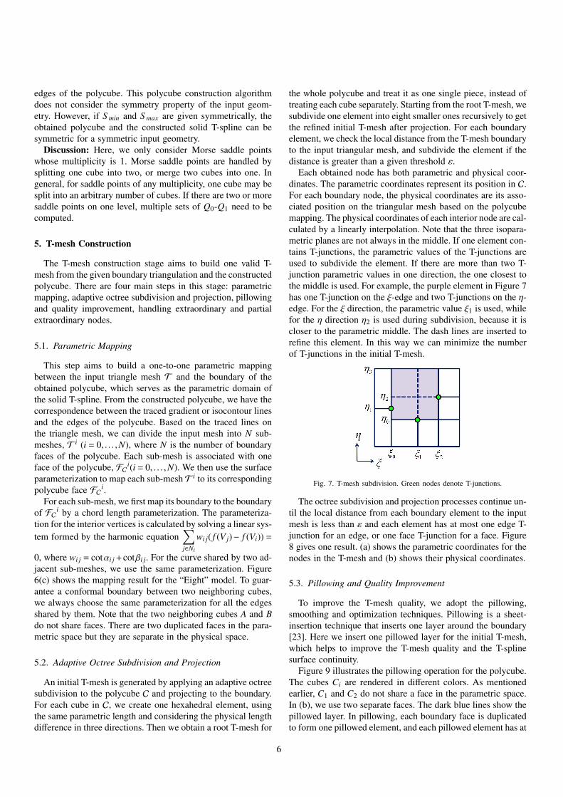
Each obtained node has both parametric and physical coor-dinates. The parametric coordinates represent its position in C.For each boundary node, the physical coordinates are its asso-ciated position on the triangular mesh based on the polycubemapping. The physical coordinates of each interior node are cal-culated by a linearly interpolation. Note that the three isopara-metric planes are not always in the middle. If one element con-tains T-junctions, the parametric values of the T-junctions areused to subdivide the element. If there are more than two T-junction parametric values in one direction, the one closest tothe middle is used. For example, the purple element in Figure 7has one T-junction on the ξ-edge and two T-junctions on the η-edge. For the ξ direction, the parametric value ξ1 is used, whilefor the η direction η2 is used during subdivision, because it iscloser to the parametric middle. The dash lines are inserted torefine this element. In this way we can minimize the numberof T-junctions in the initial T-mesh.

Fig. 7. T-mesh subdivision. Green nodes denote T-junctions.

The octree subdivision and projection processes continue un-til the local distance from each boundary element to the inputmesh is less than ε and each element has at most one edge T-junction for an edge, or one face T-junction for a face. Figure8 gives one result. (a) shows the parametric coordinates for thenodes in the T-mesh and (b) shows their physical coordinates.

5.3. Pillowing and Quality Improvement

To improve the T-mesh quality, we adopt the pillowing,smoothing and optimization techniques. Pillowing is a sheet-insertion technique that inserts one layer around the boundary[23]. Here we insert one pillowed layer for the initial T-mesh,which helps to improve the T-mesh quality and the T-splinesurface continuity.

Figure 9 illustrates the pillowing operation for the polycube.The cubes Ci are rendered in different colors. As mentionedearlier, C1 and C2 do not share a face in the parametric space.In (b), we use two separate faces. The dark blue lines show thepillowed layer. In pillowing, each boundary face is duplicatedto form one pillowed element, and each pillowed element has at

6

(c)

(a) (b) (d)

Fig. 8. The subdivision, projection, pillowing and optimization results for the“Eight” model. (a) The subdivision result in the parametric domain; (b) theinitial T-mesh; (c-d) Interior of the T-mesh before and after pillowing andoptimization.

most one face lying on the boundary. For the pillowed layer, theedge knot interval is a predefined constant along the pillowingdirection, which stays the same for the other two directions.

As shown in Figure 9(b), after pillowing the yellow cor-ner nodes become interior extraordinary nodes. The nodes onthe blue polycube edges become interior partial extraordinarynodes. The red corner nodes, pillowed from the yellow nodes,are extraordinary nodes on the boundary surface. The con-structed T-spline surface is C0-continuous around these redboundary extraordinary nodes up to the 2-ring neighborhood,C1-continuous from the 2-ring to 3-ring neighborhood, and C2-continuous everywhere else. Note that after pillowing, the sur-face continuity across the polycube edges is improved from C0

to C2. The interior region is C0-continuous around each interiorextraordinary node until the 3-ring neighborhood. For the inte-rior region across the polycube edges, the continuity is C0 untilthe 2-ring neighborhood, C1 from 2-ring to 3-ring neighbor-hood, and C2 everywhere else. Since here we introduce someextraordinary and partial extraordinary nodes, we use a localparameterization for each element in the following steps.

After pillowing, smoothing and optimization are used to im-prove the T-mesh quality. For smoothing, each node is movedtoward its mass center, and for optimization each node is movedtoward an optimal position that maximizes the worst Jacobian.For one T-mesh element, the Jacobian is defined as

J = det(JM) =

∣∣∣∣∣∣∣∣∣∣∣∣∣∣∣∣∣∣∣∣∣∣

7∑i=0

xi∂Ni

∂ξ

7∑i=0

xi∂Ni

∂η

7∑i=0

xi∂Ni

∂ζ7∑

i=0

yi∂Ni

∂ξ

7∑i=0

yi∂Ni

∂η

7∑i=0

yi∂Ni

∂ζ7∑

i=0

zi∂Ni

∂ξ

7∑i=0

zi∂Ni

∂η

7∑i=0

zi∂Ni

∂ζ

∣∣∣∣∣∣∣∣∣∣∣∣∣∣∣∣∣∣∣∣∣∣, (4)

(a) (b)

Fig. 9. The polycube before (a) and after (b) pillowing.

where Ni is a trilinear shape function. The scaled Jacobian is

Js =J

‖ JM(·,0) ‖ ‖ JM(·,1) ‖ ‖ JM(·,2) ‖, (5)

where JM(·,0), JM(·,1) and JM(·,2) represent the first, secondand last column of the Jacobian matrix, JM , respectively. Tohandle T-junctions during smoothing and optimization, we addsome “virtual nodes” to refine the local region and convert thelocal T-mesh to a hexahedral mesh. Figure 8(d) shows the resultafter pillowing and optimization for the “Eight” model.

5.4. Handling extraordinary and partial extraordinary nodes

Unlike regular nodes, extraordinary nodes or partial extraor-dinary nodes may introduce gaps to the solid T-spline. In thisstep, we apply templates given in [22] to make the T-mesh gap-free. Figure 10(a) shows the template for a partial extraordinarynode, in which the magenta edge has a reflection edge. Figure10(b) shows one general template for an extraordinary node.

(a) (b)

Fig. 10. The general template for a partial extraordinary node (a) and anextraordinary node (b). The magenta node is a partial extraordinary node,the red one is an extraordinary node, and the blue ones are inserted nodes.The magenta edge is the edge with a reflection edge and the red edges havezero knot interval.

6. Solid T-spline Construction and Bezier Extraction

In this stage, we aim to infer the local knot vectors for eachnode, build the rational solid T-spline from the T-mesh, andthen extract embedded Bezier elements [2, 15]. The concept

7

of rational T-splines was given in [22], with basis functionssatisfying a partition of unity by definition. The rational solidT-spline is defined as

S (ξ,η,ζ) =

n∑i=0

wiCiRi(ξ,η,ζ)

n∑i=0

wiRi(ξ,η,ζ)

, (ξ,η,ζ) ∈Ω, (6)

where

Ri(ξ,η,ζ) =Nξ

i (ξ)Nηi (η)Nζ

i (ζ)∑nj=0 Nξ

j (ξ)Nηj (η)Nζ

j (ζ)(7)

is the rational B-spline basis function, Nξi , Nη

i and Nζi are B-

spline basis functions defined by the local knot vectors at nodeCi which, for degree d = 3, are given by ~ξi = [ξi0, ξi1, ξi2, ξi3,ξi4], ~ηi = [ηi0, ηi1, ηi2, ηi3, ηi4] and ~ζi = [ζi0, ζi1, ζi2, ζi3, ζi4].

From the T-mesh, we first compute the knot intervals foreach node by traversing T-mesh edges and faces. Note that werepeat knots whenever we meet an extraordinary node duringthe traverse. Then for each domain, we determine all the nodeswith non-zero basis functions and use them to build the solidT-spline element. The entire solid T-spline model is built bylooping over all the local domains.

Bezier extraction provides a finite element representation ofT-splines for isogeometric analysis. Similar to [23], we firstcompute the “Bezier mesh”, which includes all the reducedcontinuity lines by adding all the knot vector inference linesor isoparametric planes for T-junctions and L-junctions to theT-mesh. Then for each element in the Bezier mesh, the trans-formation matrix Me between the T-spline basis functions andthe Bezier basis functions is calculated satisfying:

Bet = MeBe

b, (8)

where Bet is the vector formed by the nonzero T-spline basis

functions in this element and Beb is the vector formed by the

trivariate Bezier basis functions.

7. Results and Isogeometric Analysis

We have applied the construction algorithm to several models(Figures 11-14). The constructed solid T-spline is tricubic andC2-continuous except in the vicinity of partial extraordinaryand extraordinary nodes. Statistics for all the tested models areshown in Table 1. The Bezier Jacobian is calculated using thescaled Jacobian at the eight Gauss quadrature points for eachBezier element. The algorithm is efficient and all the resultswere computed on a PC equipped with an Intel X3470 processorand 8GB main memory.

The Isis model has genus zero and its polycube only con-tains one single cube. For the kitten model, there are three sad-dle points (one merging saddle point and two splitting saddlepoints). We only consider two of them, and the splitting sad-dle point close to the maximum point is skipped to get a moresimplified polycube. The sculpture model has genus two and

(a) (b) (c)

Fig. 11. The solid T-spline construction result for the “Eight” model. (a) Theconstructed solid T-spline and T-mesh; (b) the extracted solid Bezier meshwith some elements removed to show the interior (blue) and one pillowedlayer (magenta); and (c) the isogeometric analysis result.

five saddle points. Again, we skipped the one near the max-imal level. The time used for each model not only dependson the input mesh size, but also depends on the T-mesh size,which is determined by the given surface error tolerance andthe complexity of the topology and geometry. One advantageof this harmonic function based T-spline construction is thatthe isoparametric lines are basically aligned with the geometricstructure of the model.

We have developed a 3D isogeometric analysis solver forstatic mechanics analysis, which uses rational T-splines as thebasis, and we used it to test the obtained solid T-spline models.For all the models, we fix all the control points on the bottomand apply unit displacement on the top. The Young’s modulusE = 72.4GPa, and the Poisson’s ratio ν = 0.3. The obtaineddisplacement results are given in Figures 11(c), 12(e), 13(g) and14(g). From these results, we can conclude that the obtainedrational T-splines can be used in isogeometric analysis directlyand reasonable simulation results can be obtained.

8. Conclusions

We have presented a new algorithm to construct solid T-splines for arbitrary-genus geometries from boundary triangu-lations. Our method is efficient and the resulting solid T-splineis analysis-suitable with C2-continuity except for the local re-gion around a few irregular nodes. In this paper, we only con-sider the geometries with Morse saddle points, and as part ofour future work we will extend the algorithm to geometrieswith arbitrary saddle points. We will also consider engineeringdesigns with sharp features.

Acknowledgements

Y. Zhang, W. Wang and L. Liu were supported in partby ONR Grant N00014-08-1-0653. T. J.R. Hughes was sup-ported by ONR Grant N00014-08-1-0992, NSF GOALI CMI-

8

(a) (b) (c) (d) (e)

(f) (g) (h)

Fig. 12. Isis model with genus zero. (a) The input boundary triangle mesh; (b) the harmonic scalar field; (c) the constructed solid T-spline and T-mesh; (d)the extracted solid Bezier elements; (e) the isogeometric analysis result; (f) the constructed polycube and the mapping result; (g) the subdivision result for theparametric domain; and (h) the extracted solid Bezier mesh with some elements removed to show the interior (blue) and one pillowed layer (magenta).

9

Table 1. Statistics of all the tested models

Model Genus Input mesh T-mesh Extraordinary nodes Interior partial Bezier Bezier Jacobian Time

(vertices, elements) nodes (Boundary, Interior) extraordinary nodes elements (worst, best) (s)

Isis 0 (5,863, 11,722) 9,310 (8, 8) 244 5,335 (0.12, 1.0) 52.0

Kitten 1 (5,377, 10,754) 4,825 (12, 12) 140 2,883 (0.08, 1.0) 14.8

Eight 2 (766, 1,536) 5,735 (16, 16) 200 1,440 (0.10, 1.00) 8.5

Sculpture 2 (8,635, 17,276) 10,549 (16, 16) 252 7,072 (0.09, 1.00) 41.5

(a) (b) (c) (d)

(e) (f) (g) (h)

Fig. 13. Kitten model with genus one. (a) The input boundary triangle mesh; (b) the harmonic scalar field; (c) the constructed polycube and the mapping result;(d) the subdivision result for the parametric domain; (e) the constructed solid T-spline and T-mesh; (f) the extracted solid Bezier elements; (g) the extractedsolid Bezier mesh with some elements removed to show the interior (blue) and one pillowed layer (magenta); and (h) the isogeometric analysis result.

10

(a) (b) (c) (d)

(e) (f)

(g)

(h)

Fig. 14. Sculpture model with genus two. (a) The input boundary triangle mesh; (b) the harmonic scalar field; (c) the constructed polycube and the mappingresult; (d) the subdivision result for the parametric domain; (e) the constructed solid T-spline and T-mesh; (f) the extracted solid Bezier elements; (g) theextracted solid Bezier mesh with some elements removed to show the interior (blue) and one pillowed layer (magenta); and (h) the isogeometric analysis result.

11

0700807/0700204, NSF CMMI-1101007 and a grant fromSINTEF. The “Eight” model is from the AIM@SHAPE ShapeRepository.

References

[1] M. Aigner, C. Heinrich, B. Juttler, E. Pilgerstorfer,B. Simeon, and A. V. Vuong. Swept volume parameter-ization for isogeometric analysis. In IMA InternationalConference on Mathematics of Surfaces XIII, pages 19–44, 2009.

[2] M. J. Borden, M. A. Scott, J. A. Evans, and T. J.R.Hughes. Isogeometric finite element data structures basedon Bezier extraction of NURBS. International Journalfor Numerical Methods in Engineering, 87:15–47, 2011.

[3] S. Dong, S. Kircher, and M. Garland. Harmonic func-tions for quadrilateral remeshing of arbitrary manifolds.Comput. Aided Geom. Des., 22:392–423, 2005.

[4] J. M. Escobar, J. M. Cascon, E. Rodrıguez, and R. Mon-tenegro. A new approach to solid modeling with trivariateT-splines based on mesh optimization. Computer Meth-ods in Applied Mechanics and Engineering, 200(45-46):3210–3222, 2011.

[5] M. S. Floater. Parametrization and smooth approxima-tion of surface triangulations. Computer Aided GeometricDesign, 14(3):231–250, 1997.

[6] M. S. Floater and K. Hormann. Surface parameterization:a tutorial and survey. Advances in Multiresolution forGeometric Modelling, pages 157–186, 2005.

[7] X. Gu and S. Yau. Global conformal surface parameteri-zation. In Eurographics/ACM SIGGRAPH symposium onGeometry processing, pages 127–137, 2003.

[8] X. Gu, Y. Wang, T.F. Chan, P.M. Thompson, and S.-T.Yau. Genus zero surface conformal mapping and its ap-plication to brain surface mapping. IEEE Transaction onMedical Imaging, 23(8):949–958, 2004.

[9] Y. He, H. Wang, C. Fu, and H. Qin. A divide-and-conquerapproach for automatic polycube map construction. Com-puters & Graphics, 33(3):369–380, 2009.

[10] J. Hua, Y. He, and H. Qin. Multiresolution heterogeneoussolid modeling and visualization using trivariate simplexsplines. In ACM Symposium on Solid Modeling and Ap-plications, pages 47–58, 2004.

[11] T. J.R. Hughes, J. A. Cottrell, and Y. Bazilevs. Isogeomet-ric analysis: CAD, finite elements, NURBS, exact geom-etry, and mesh refinement. Computer Methods in AppliedMechanics and Engineering, 194:4135–4195, 2005.

[12] T. Kanai, H. Suzuki, and F. Kimura. 3D geometric meta-morphosis based on harmonic maps. In Pacific Graphics,pages 97–104, 1997.

[13] B. Li, X. Li, K. Wang, and H. Qin. Generalized poly-cube trivariate splines. In Shape Modeling InternationalConference, pages 261–265, 2010.

[14] T. Martin, E. Cohen, and R. M. Kirby. Volumetric pa-rameterization and trivariate B-spline fitting using har-monic functions. Computer Aided Geometric Design, 26

(6):648–664, 2009.[15] M. A. Scott, M. J. Borden, C. V. Verhoosel, T. W. Seder-

berg, and T. J.R. Hughes. Isogeometric finite element datastructures based on Bezier extraction of T-splines. Inter-national Journal for Numerical Methods in Engineering,88(2):126–156, 2011.

[16] T. W. Sederberg, J. Zheng, A. Bakenov, and A. Nasri. T-splines and T-NURCCs. ACM Transactions on Graphics,22(3):477–484, 2003.

[17] T. W. Sederberg, D. L. Cardon, G. T. Finnigan, N. S.North, J. Zheng, and T. Lyche. T-spline simplification andlocal refinement. In ACM SIGGRAPH, pages 276–283,2004.

[18] A. Sheffer, E. Praun, and K. Rose. Mesh parameterizationmethods and their applications. Found. Trends. Comput.Graph. Vis., 2:105–171, 2006.

[19] M. Tarini, K. Hormann, P. Cignoni, and C. Montani.Polycube-maps. ACM Trans. Graph., 23(3):853–860,2004.

[20] H. Wang, Y. He, X. Li, X. Gu, and H. Qin. Polycubesplines. In Symposium on Solid and Physical Modeling,pages 241–251, 2007.

[21] K. Wang, X. Li, B. Li, H. Xu, and H. Qin. Restrictedtrivariate polycube splines for volumetric data modeling.IEEE Transactions on Visualization and Computer Graph-ics, 18:703–716, 2012.

[22] W. Wang, Y. Zhang, G. Xu, and T. J.R. Hughes. Convert-ing an unstructured quadrilateral/hexahedral mesh to a ra-tional T-spline. Computational Mechanics, (2012) DOI:10.1007/s00466-011-0674-6.

[23] Y. Zhang, W. Wang, and T. J.R. Hughes. SolidT-spline construction from boundary representationsfor genus-zero geometry. Computer Methods inApplied Mechanics and Engineering, (2012) DOI:10.1016/j.cma.2012.01.014.

[24] Y. Zhang, Y. Bazilevs, S. Goswami, C. L. Bajaj, and T. J.R.Hughes. Patient-specific vascular NURBS modeling forisogeometric analysis of blood flow. Computer Methods inApplied Mechanics and Engineering, 196(29-30):2943–2959, 2007.

12