icesat full-waveform altimetry compared to airborne laser

IEEE TRANSACTIONS ON GEOSCIENCE AND REMOTE SENSING, VOL. 47, NO. 10, OCTOBER 2009 3365

ICESat Full-Waveform Altimetry Comparedto Airborne Laser Scanning Altimetry

Over The NetherlandsHieu Duong, Associate Member, IEEE, Roderik Lindenbergh, Norbert Pfeifer, and George Vosselman

Abstract—Since 2003, the full-waveform laser altimetry systemonboard NASA’s Ice, Cloud and land Elevation Satellite (ICESat)has acquired a worldwide elevation database. ICESat data arewidely applied for change detection of ice sheet mass balance,forest structure estimation, and digital terrain model generationof remote areas. ICESat’s measurements will be continued by afollow-up mission. To fully assess the application possibilities of thefull-waveform products of these missions, this research analyzesthe vertical accuracy of ICESat products over complex terrainwith respect to land cover type. For remote areas, validationof individual laser shots is often beyond reach. For a countrywith extensive geo-infrastructure such as The Netherlands, ex-cellent countrywide validation is possible. Therefore, the ICESatfull-waveform product GLA01 and the land elevation productGLA14 are compared to data from the Dutch airborne laseraltimetry archive Actual Height model of the Netherlands (AHN).For a total population of 3172 waveforms, differences betweenICESat- and AHN-derived terrain heights are determined. The av-erage differences are below 25 cm over bare land and urban areas.Over forests, differences are even smaller but with slightly largerstandard deviations of about 60 cm. Moreover, a waveform-basedfeature height comparison resulted in feature height differencesof 1.89 m over forest, 1.48 m over urban areas, and 29 cm overlow vegetation. These results, in combination with the presentedprocessing chain and individual waveform examples, show thatstate-of-the-art ICESat waveform processing is able to analyzewaveforms at the individual shot level, particularly outside urbanareas.

Index Terms—Actual height model of The Netherlands (AHN),digital terrain models (DTMs), feature height, full waveform, Ice,Cloud and land Elevation Satellite (ICESat), laser altimetry.

I. INTRODUCTION

THE ICE, Cloud and land Elevation Satellite (ICESat)was launched in January 2003 to observe the cryosphere

and atmosphere and to measure land topography profiles and

Manuscript received June 6, 2008; revised February 19, 2009 and April 3,2009. First published June 23, 2009; current version published September 29,2009. This work was supported by the Delft Research Centre “Earth.”

H. Duong and R. Lindenbergh are with the Delft University of Tech-nology, 2629 HS Delft, The Netherlands (e-mail: [email protected];[email protected])

N. Pfeifer is with the Institute of Photogrammetry and Remote Sens-ing, Vienna University of Technology, 1040 Vienna, Austria (e-mail:[email protected]).

G. Vosselman is with the International Institute for Geo-Information Scienceand Earth Observation (ITC), 7500 AA Enschede, The Netherlands (e-mail:[email protected]).

Color versions of one or more of the figures in this paper are available onlineat http://ieeexplore.ieee.org.

Digital Object Identifier 10.1109/TGRS.2009.2021468

canopy heights [1]. These objectives are accomplished usingthe Geoscience Laser Altimeter System (GLAS), in combi-nation with precise orbit determination (POD) and precisealtitude determination (PAD). Since 2003, ICESat has acquireda huge database of raw and processed data organized in 15 dataproducts, i.e., GLA01, . . ., GLA15 [2]. Each product contains adifferent data type. For example, the GLA01 level-1A productcontains the raw full-waveform data, and the GLA14 productprovides global land surface elevation data [3].

ICESat data products have been used in many researchtopics in recent years. Typical applications include forestry(such as estimation of canopy parameters and above-groundbiomass [4]–[6], vegetation vertical structure [7]–[9], forestdisturbance [10], and single- and two-epoch analyses of ICESatfull-waveform data over forested areas [11]) and polar regions,accuracy and precision of digital elevation models (DEMs)[12], [13], mass balance over Antarctica [14], volume changerate of the ice sheet over Greenland [15], snow accumulationon ice sheets [16], and estimation of sea ice thickness by usingsnow depth on the sea ice [17]. Follow-up missions are plannedto continue the acquisition of large footprint waveform data.ICESat-II and the scheduled Deformation, Ecosystem Structureand Dynamics of Ice (DESDynI) mission will also operate alarge footprint waveform system.

To obtain insight into ICESat data accuracy, ICESat datawere compared and validated by independent data sources.ICESat data were several times compared with data of mod-erate accuracy, such as InSAR-derived DEMs [18] and ShuttleRadar Topography Mission (SRTM) data [19]–[21]. Elevationdifferences between ICESat data and SRTM data are discussedeither with respect to different land cover types, as derivedfrom Landsat-7 images [21], or over high relief and denselyvegetated surfaces [19], [20]. In addition, the highest and lowestelevations derived from the ICESat full-waveform data are alsodiscussed in [19] and [20] to assess the properties of ICESatdata over complex land surfaces.

ICESat data are also carefully compared with more accuratedata, such as airborne laser scanning data [22]–[24] and GlobalPositioning System measurements [25]–[27]. According to[25], ICESat-derived elevations are impacted by environmentaleffects (e.g., forward scattering and surface reflectance) andinstrument effects (e.g., pointing biases, detector saturation, andvariations in transmitted laser energy). Under ideal conditions,a vertical bias of less than 2 cm with a standard deviation of atleast 3 cm is reported [22]–[25].

0196-2892/$26.00 © 2009 IEEE

Authorized licensed use limited to: TU Delft Library. Downloaded on July 06,2010 at 11:46:57 UTC from IEEE Xplore. Restrictions apply.

3366 IEEE TRANSACTIONS ON GEOSCIENCE AND REMOTE SENSING, VOL. 47, NO. 10, OCTOBER 2009

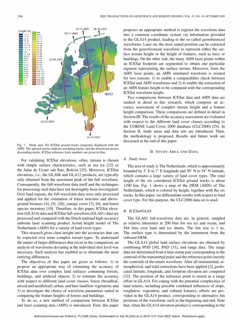
Fig. 1. Study area. Six ICESat ground tracks (magenta) displayed with theAHN. The upward arrows indicate ascending tracks, and the downward arrowsdescending tracks. ICESat reference track numbers are given in blue.

For validating ICESat elevations, often, terrain is chosenwith simple surface characteristics, such as sea ice [22] orthe Salar de Uyuni salt flats, Bolivia [25]. Moreover, ICESatelevations, i.e., the GLA06 and GLA12 products, are typicallyonly obtained from the maximum peak of the full waveform.Consequently, the full-waveform data itself and the techniquesfor processing such data have not thoroughly been investigated.Over land regions, the full-waveform data were only processedand applied for the estimation of forest structure and above-ground biomass [4], [5], [28], canopy cover [7], [8], and forestspecies inventory [10]. Therefore, in this paper, ICESat eleva-tion (GLA14) data and ICESat full-waveform (GLA01) data areprocessed and compared with the Dutch national high-accuracyairborne laser scanning product Actual height model of TheNetherlands (AHN) for a variety of land cover types.

This research gives clear insight into the accuracies that canbe expected over more complex terrain types. To understandthe nature of larger differences that occur in the comparison, ananalysis of waveforms deviating at the individual shot level wasnecessary. Such analysis has enabled us to eliminate the mostoutlying differences.

The objectives of this paper are given as follows: 1) topropose an appropriate way of estimating the accuracy ofICESat data over complex land surfaces containing forests,buildings, and artificial objects; 2) to estimate the accuracywith respect to different land cover classes: forest (broadleaf,mixed and needleleaf), urban, and bare land/low vegetation; and3) to investigate the choice of waveform parameters suited incomparing the feature heights of forests and buildings.

To do so, a new method of comparison between ICESatand laser scanning data (AHN) is introduced. First, this paper

proposes an appropriate method to register the waveform datainto a common coordinate system via information providedin the GLA14 product, leading to the so-called georeferencedwaveforms. Later on, the most suited position can be extractedfrom the georeferenced waveform to represent either the sur-face terrain height or the height of features, such as trees orbuildings. On the other side, the many AHN laser points withinan ICESat footprint are segmented to obtain one particularsegment representing the surface terrain. Moreover, from theAHN laser points, an AHN simulated waveform is createdfor two reasons: 1) to enable a comparability check betweenICESat and AHN waveforms and 2) to enable the extraction ofan AHN feature height to be compared with the correspondingICESat waveform height.

Two comparisons between ICESat data and AHN data arestudied in detail in this research, which comprise an ac-curacy assessment of complex terrain height and a featureheight comparison. These comparisons are defined in detail inSection III. The results of the accuracy assessment are evaluatedwith respect to the different land cover classes according tothe CORINE Land Cover 2000 database (CLC2000) [29]. InSection II, study areas and data sets are introduced. Then,the methodology is proposed. Results and future work arediscussed at the end of this paper.

II. STUDY AREA AND DATA

A. Study Area

The area of study is The Netherlands, which is approximatelybounded by 3◦ E to 7◦ E longitude and 50◦ N to 54◦ N latitude,which contains a large variety of land cover types. The totallength of the six considered ICESat ground tracks is about1290 km. Fig. 1 shows a map of the DEM (AHN) of TheNetherlands, which is colored by height, together with the sixtracks. In this paper, we differentiate results with respect to landcover type. For this purpose, the CLC2000 data set is used.

B. ICESat/GLAS

The GLA01 full-waveform data are, in general, sampledas relative intensities in 200 bins for sea ice and ocean, and544 bins over land and ice sheets. The bin size is 1 ns.The surface type is determined by the instrument from theonboard DEM.

The GLA14 global land surface elevations are obtained bycombining POD [30], PAD [31], and range data. The rangedata are determined from a time stamp pair corresponding to thecentroid of the transmitted pulse and the reference point (mostlythe centroid) of the return waveform. After all instrumental, at-mospherical, and tidal corrections have been applied [2], geolo-cated latitude, longitude, and footprint elevation are computed[32]. The position of the reference point is stored as a rangeoffset in GLA14. For coping with the potential complexities ofland returns, including possible combined influences of slope,roughness, vegetation, and cultural features, offsets are pro-vided in the GLA14 product, corresponding to alternative binpositions of the waveform, such as the beginning and end. Notethat, when the GLA14 elevation product is corresponding to the


DUONG et al.: ICESat FULL-WAVEFORM ALTIMETRY 3367

TABLE INUMBER OF ICESAT WAVEFORMS USED: FOREST (BROADLEAF, MIXED, AND NEEDLELEAF), URBAN, BARE LAND, AND WATER

waveform centroid, it is representing the mean elevation withinthe illuminated footprint [7]. In addition, ICESat waveformsthat cause saturation of the ICESat detector result in a lowerelevation [25]. A saturation elevation correction i_satElevCorris applied to all GLA14 data.

To avoid large changes in surface features and land coverbecause of acquisition time differences, the acquisition time ofICESat data needs to be close to the acquisition time of theAHN data (1996–2003) and the CLC2000 data (1999–2001).Therefore, ICESat GLA14 and GLA01 products from cam-paign L2a, which were obtained in the period betweenSeptember 25, 2003 and November 18, 2003, are chosen for thisstudy. As a result, the difference in acquisition time betweenthe data considered varies from 0 to 7 years. All data are fromrelease 428, and the waveform data were digitized in 544 bins.In Table I, the orientation and length of the major and minoraxes of the ellipses describing the footprint shape are given foreach track.

These six ICESat ground tracks are chosen because of fourreasons.

1) To be well spatially distributed over the study area.2) To cover all different land cover classes.3) ICESat measurements along these six tracks were rela-

tively successful, compared with other L2a tracks (cloudcover).

4) For some of the tracks also considered, repeated tracks insubsequent campaigns are available (tracks 0015, 0043,and 0295), which allows repeating this analysis for latercampaigns.

Moreover, waveforms from overlapping footprints from re-peated tracks can be compared to assess terrain height changesand feature height changes and to identify further issues inthe processing of ICESat data (cf. [33]). Starting 2007, AHN2is being acquired over The Netherlands [34]. AHN2 has evenbetter specifications than the first version of AHN used in thisstudy. The release of AHN2 will offer good possibilities toassess the quality of the most recent ICESat campaigns.

After applying filtering constraints, as described later inSection III-G, a total of 3172 waveforms from six ICESattracks were assigned to different land cover classes by usingthe CLC2000 land cover database (Table I). The transmittedenergy falls from 81 to 66 mJ during the campaign. The averagereturn energy of the waveform from each track varies from

17 to 316 fJ. Moreover, the nominal pointing angle is alwaysabout 0.3◦. According to [35], given the reported pointing errorof 0 ± 1.5 arcsec in data campaign L2a, ICESat elevation datahave a theoretically vertical accuracy of 2.25 cm/1◦ incidentangle and a horizontal accuracy of 4.5 m [35].

C. AHN

The AHN was acquired between 1996 and 2003 under leaf-off conditions and is based on airborne laser altimetry, with apoint density of at least 1 point per 4 × 4 m2 area. There arefour levels of detail available, i.e., raw point cloud data andinterpolated grid data at 5-, 25-, and 100-m resolution [34],[36]. In this study, the raw point cloud data are used. Overrural areas, the raw point cloud data are divided into nongroundpoints (so-called vegetation points) and ground points. Overurban areas, no filtering is applied. Hence, both vegetation andbuildings are present in the urban AHN data sets. All data are inASCII format files with XY Z coordinates given in the Dutchcoordinate system Rijksdriehoeksmeting and Normaal Amster-dams Peil (RDNAP) [37]. The accuracy strongly depends on theamount of vegetation and topography. For solid surfaces (e.g.,roads and parking lots) and soft but flat surfaces (e.g., beachesand grass fields), the maximum systematic offset is 5 cm with astandard deviation of 15 cm. Over wooded areas, the maximumsystematic offset is 10 cm with a standard deviation of 20 cm incase of at least one ground point per 36 m2 [34].

D. CLC2000

The CLC2000 was developed by the European Environ-ment Agency and the European Joint Research Centre. TheCLC2000 database originates from the year 2000 but is actu-ally obtained during a three-year period from 1999 to 2001,with a horizontal geolocation accuracy of 25 m based onsatellite images of Landsat-7 Enhanced Thematic MapperPlus with 25-m pixel resolution. The CLC2000 data prod-uct is obtained from Landsat data via a computer-assistedvisual interpretation of the satellite images, under the re-quirements of a scale of 1 : 100 000, a minimum mappingunit of 25 ha, and a pixel resolution of 100 m [38].The CLC2000 classification is hierarchical and distinguishes44 classes at the third level, 15 classes at the second level, andfive classes at the first level. Detailed information of land coverlevels can be found on the metadata section on the European



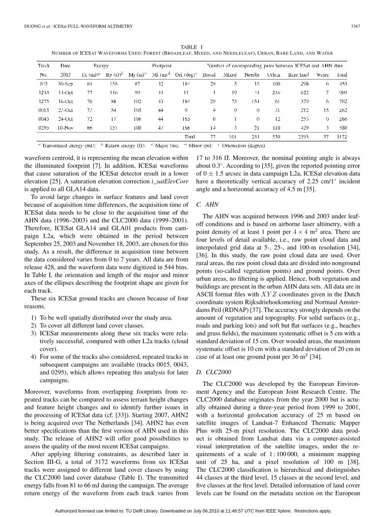
Fig. 2. Procedure of coordinate system conversion.

Environment Agency website [29]. The total thematic accuracyof the CLC2000 database was almost 95%. The database isgeoreferenced in the European reference system (ERS) [39].

III. METHODOLOGY

A. Datum Transformation and Coordinate Systems

A critical step in the elevation comparison is coordinatesystem conversion. For comparison between ICESat and AHNdata with respect to land cover type from CLC2000, data setsneed to be available in the same georeferenced coordinatesystem. AHN and CLC2000 data are available in RDNAPand ERS coordinates, respectively. Because AHN data andCLC2000 are very large data sets, ICESat data that are ini-tially in the TOPEX/Poseidon reference frame, are chosento be converted. ICESat data are both converted to RDNAPand ERS coordinates. The conversion scheme is shown inFig. 2. The ICESat data in the TOPEX/Poseidon ellipsoid arefirst converted to the WGS84 ellipsoid by Interactive DataLanguage scripts provided by NSIDC [40]. This conversionproduced a very small error of less than 1 cm [41]. Then,the ICESat data in WGS84 coordinates are converted to theETRS89 reference system by the program PCTrans 4.0 [42].The accuracy of this step is up to the centimeter level. Next,these data are transformed to the RDNAP system by theCoordinate Calculator developed in [37]. This conversion isaccurate within 1 cm [43]. The total accuracy of the previoussteps is still restricted to the centimeter level; therefore, thiserror component cannot be considered very significant to thecomparison. Moreover, the ICESat GLA14 data in ETRS89system are additionally converted to the ERS coordinates byArcGIS 9.2 [44]. The ICESat geolocation accuracy of about4.5 m is well below the CLC2000 resolution of 100 m. There-fore, this conversion has no significant effect either. Finally,the ICESat data are assigned to land cover type classes bycomparison to the CLC2000.

B. Georeferenced Waveform

Typically, one position on the time axis of each waveformis used to compute a range between the GLAS sensor and theEarth surface, which is the so-called reference point. Togetherwith the ICESat orbit position and orientation, elevation data,such as that available in GLA14, can be obtained [32]. To beable to use different positions in one waveform for differentcomparisons, this paper proposes a two-step approach: First,a waveform is registered into the RDNAP coordinate systemusing the reference point (the waveform centroid in most cases).

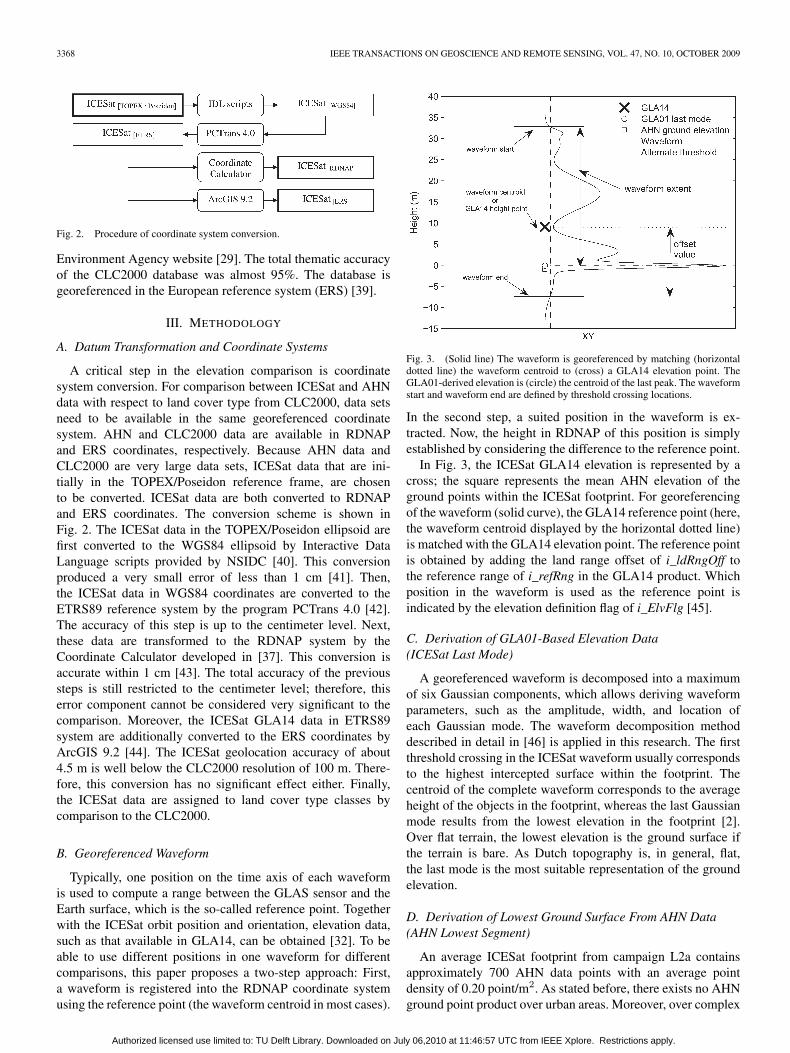
Fig. 3. (Solid line) The waveform is georeferenced by matching (horizontaldotted line) the waveform centroid to (cross) a GLA14 elevation point. TheGLA01-derived elevation is (circle) the centroid of the last peak. The waveformstart and waveform end are defined by threshold crossing locations.

In the second step, a suited position in the waveform is ex-tracted. Now, the height in RDNAP of this position is simplyestablished by considering the difference to the reference point.

In Fig. 3, the ICESat GLA14 elevation is represented by across; the square represents the mean AHN elevation of theground points within the ICESat footprint. For georeferencingof the waveform (solid curve), the GLA14 reference point (here,the waveform centroid displayed by the horizontal dotted line)is matched with the GLA14 elevation point. The reference pointis obtained by adding the land range offset of i_ldRngOff tothe reference range of i_refRng in the GLA14 product. Whichposition in the waveform is used as the reference point isindicated by the elevation definition flag of i_ElvFlg [45].

C. Derivation of GLA01-Based Elevation Data(ICESat Last Mode)

A georeferenced waveform is decomposed into a maximumof six Gaussian components, which allows deriving waveformparameters, such as the amplitude, width, and location ofeach Gaussian mode. The waveform decomposition methoddescribed in detail in [46] is applied in this research. The firstthreshold crossing in the ICESat waveform usually correspondsto the highest intercepted surface within the footprint. Thecentroid of the complete waveform corresponds to the averageheight of the objects in the footprint, whereas the last Gaussianmode results from the lowest elevation in the footprint [2].Over flat terrain, the lowest elevation is the ground surface ifthe terrain is bare. As Dutch topography is, in general, flat,the last mode is the most suitable representation of the groundelevation.

D. Derivation of Lowest Ground Surface From AHN Data(AHN Lowest Segment)

An average ICESat footprint from campaign L2a containsapproximately 700 AHN data points with an average pointdensity of 0.20 point/m2. As stated before, there exists no AHNground point product over urban areas. Moreover, over complex



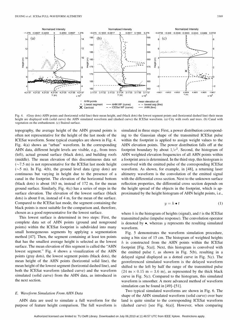
Fig. 4. (Gray dots) AHN points and (horizontal solid line) their mean height, and (black dots) the lowest segment points and (horizontal dashed line) their meanheight are displayed with (solid curve) the AHN simulated waveform and (dashed curve) the ICESat waveform. (a) City with roofs and trees. (b) Canal withvegetation on the embankment. (c) Staired surface.

topography, the average height of the AHN ground points isoften not representative for the height of the last mode of theICESat waveform. Some typical examples are shown in Fig. 4.Fig. 4(a) shows an “urban” waveform. In the correspondingAHN data, different height levels are visible, e.g., from trees(left), actual ground surface (black dots), and building roofs(middle). The mean elevation of this discontinuous data set(∼7.5 m) is not representative for the ICESat last mode height(∼5 m). In Fig. 4(b), the ground level data (gray dots) arecontinuous but varying in height due to the presence of acanal in the footprint. The elevation of the horizontal bottom(black dots) is about 163 m, instead of 172 m, for the meanground surface. Similarly, Fig. 4(c) has a series of steps in thesurface elevation. The elevation of the lowest surface (blackdots) is about 0 m, instead of 4 m, for the mean of the surface.Compared to the ICESat last mode, the segment containing theblack points is most suitable for the comparison and, therefore,chosen as a good representative for the lowest surface.

This lowest surface is determined in two steps: First, thecomplete data set of AHN points (ground and nongroundpoints) within the ICESat footprint is subdivided into manysmall homogeneous segments by applying a segmentationmethod [47]. Then, the segment containing at least ten pointsthat has the smallest average height is selected as the lowestsurface. The mean elevation of this segment is called the “AHNlowest segment.” Fig. 4 shows a visualization of the AHNpoints (gray dots), the lowest segment points (black dots), themean height of the AHN points (horizontal solid line), themean height of the lowest segment (horizontal dashed line), andboth the ICESat waveform (dashed curve) and the waveformsimulated (solid curve) from the AHN data, as introduced inthe next section.

E. Waveform Simulation From AHN Data

AHN data are used to simulate a full waveform for thepurpose of feature height comparison. The full waveform is

simulated in three steps: First, a power distribution correspond-ing to the Gaussian shape of the transmitted ICESat pulsewithin the footprint is applied to assign weight values to theAHN elevation points. The power distribution falls off at thefootprint boundary by about 1/e2. Second, the histogram ofAHN weighted elevation frequencies of all AHN points withina footprint area is determined. In the third step, this histogram isconvolved with the emitted pulse of the corresponding ICESatwaveform. As shown, for example, in [48], a returning laseraltimetry waveform is the convolution of the emitted signalwith the differential cross section. Next to the unknown surfacereflection properties, the differential cross section depends onthe height spread of the objects in the footprint, which is ap-proximated by the height histogram of AHN height points, i.e.,

y = h • t (1)

where h is the histogram of heights (signal), and t is the ICESattransmitted pulse (impulse response). The convolution operatoris denoted by •, whereas y represents the resulting simulatedwaveform.

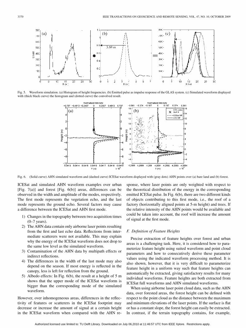
Fig. 5 demonstrates the waveform simulation procedure,using a bin size of 15 cm. The histogram of weighted heightsh is constructed from the AHN points within the ICESatfootprint [Fig. 5(a)]. Next, this histogram is convolved withthe emitted pulse t, as shown in Fig. 5(b), resulting in adelayed signal displayed as a dotted curve in Fig. 5(c). Thegeoreferenced simulated waveform is the delayed waveformshifted to the left by half the range of the transmitted pulse(24 ns × 0.15 m = 3.6 m), as represented by the thick blackcurve in Fig. 5(c). Compared to the histogram, this simulatedwaveform is smoother. A more advanced method of waveformsimulation can be found in [49]–[51].

Two typical simulated waveforms are shown in Fig. 6. Theshape of the AHN simulated waveform (solid curve) over bareland is quite similar to the corresponding ICESat waveform(dashed curve) [see Fig. 6(a)]. However, when comparing



Fig. 5. Waveform simulation. (a) Histogram of height frequencies. (b) Emitted pulse as impulse response of the GLAS system. (c) Simulated waveform displayedwith (thick black curve) the histogram and (dotted curve) the convolved result.

Fig. 6. (Solid curve) AHN simulated waveform and (dashed curve) ICESat waveform displayed with (gray dots) AHN points over (a) bare land and (b) forest.

ICESat and simulated AHN waveform examples over urban[Fig. 7(a)] and forest [Fig. 6(b)] areas, differences can beobserved in the width and amplitude of the modes, respectively.The first mode represents the vegetation echo, and the lastmode represents the ground echo. Several factors may causea difference between the ICESat and AHN first mode.

1) Changes in the topography between two acquisition times(0–7 years).

2) The AHN data contain only airborne laser points resultingfrom the first and last echo data. Reflections from inter-mediate scatterers were not available. This may explainwhy the energy of the ICESat waveform does not drop tothe same low level as the simulated waveform.

3) Contamination of the AHN data by multipath effects orindirect reflections.

4) The differences in the width of the last mode may alsodepend on the season. If most energy is reflected in thecanopy, less is left for reflection from the ground.

5) Albedo effects: In Fig. 6(b), the result at a height of 5 mshows that the upper mode of the ICESat waveform isbigger than the corresponding mode of the simulatedwaveform.

However, over inhomogeneous areas, differences in the reflec-tivity of features or scatterers in the ICESat footprint maydecrease or increase the amount of signal at a certain heightin the ICESat waveform when compared with the AHN re-

sponse, where laser points are only weighted with respect tothe theoretical distribution of the energy in the correspondingemitted ICESat pulse. In Fig. 6(b), there are two different kindsof objects contributing to this first mode, i.e., the roof of afactory (horizontally aligned points at 5-m height) and trees. Ifthe relative intensity of the AHN points would be available andcould be taken into account, the roof will increase the amountof signal at the first mode.

F. Definition of Feature Heights

Precise extraction of feature heights over forest and urbanareas is a challenging task. Here, it is considered how to para-meterize feature height using suited waveform and point cloudparameters and how to consecutively derive these parametervalues using the indicated waveform processing method. It isalso shown, however, that it is very difficult to parameterizefeature height in a uniform way such that feature heights canautomatically be extracted, giving satisfactory results for manyindividual waveforms. Feature heights are both extracted fromICESat full waveforms and AHN simulated waveforms.

When using airborne laser point cloud data, such as the AHNdata, over forested areas, the forest height can be defined withrespect to the point cloud as the distance between the maximumand minimum elevations of the laser points. If the surface is flator has a constant slope, the forest height can easily be extracted.In contrast, if the terrain topography contains, for example,



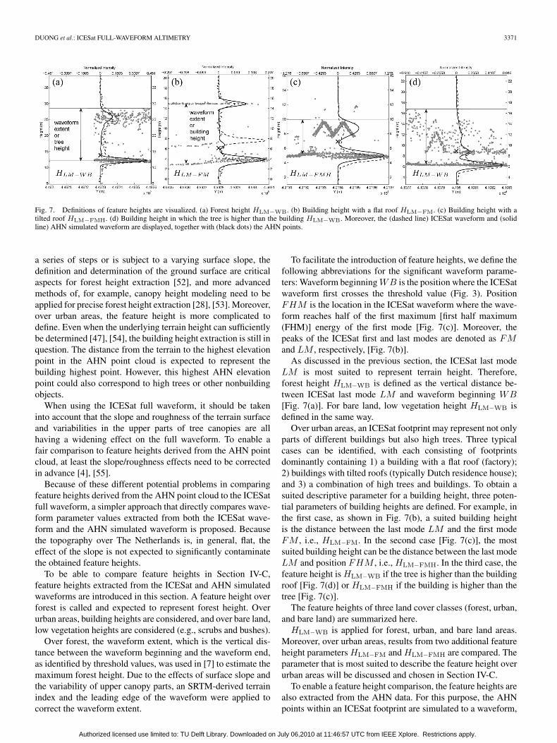
Fig. 7. Definitions of feature heights are visualized. (a) Forest height HLM−WB. (b) Building height with a flat roof HLM−FM. (c) Building height with atilted roof HLM−FMH. (d) Building height in which the tree is higher than the building HLM−WB. Moreover, the (dashed line) ICESat waveform and (solidline) AHN simulated waveform are displayed, together with (black dots) the AHN points.

a series of steps or is subject to a varying surface slope, thedefinition and determination of the ground surface are criticalaspects for forest height extraction [52], and more advancedmethods of, for example, canopy height modeling need to beapplied for precise forest height extraction [28], [53]. Moreover,over urban areas, the feature height is more complicated todefine. Even when the underlying terrain height can sufficientlybe determined [47], [54], the building height extraction is still inquestion. The distance from the terrain to the highest elevationpoint in the AHN point cloud is expected to represent thebuilding highest point. However, this highest AHN elevationpoint could also correspond to high trees or other nonbuildingobjects.

When using the ICESat full waveform, it should be takeninto account that the slope and roughness of the terrain surfaceand variabilities in the upper parts of tree canopies are allhaving a widening effect on the full waveform. To enable afair comparison to feature heights derived from the AHN pointcloud, at least the slope/roughness effects need to be correctedin advance [4], [55].

Because of these different potential problems in comparingfeature heights derived from the AHN point cloud to the ICESatfull waveform, a simpler approach that directly compares wave-form parameter values extracted from both the ICESat wave-form and the AHN simulated waveform is proposed. Becausethe topography over The Netherlands is, in general, flat, theeffect of the slope is not expected to significantly contaminatethe obtained feature heights.

To be able to compare feature heights in Section IV-C,feature heights extracted from the ICESat and AHN simulatedwaveforms are introduced in this section. A feature height overforest is called and expected to represent forest height. Overurban areas, building heights are considered, and over bare land,low vegetation heights are considered (e.g., scrubs and bushes).

Over forest, the waveform extent, which is the vertical dis-tance between the waveform beginning and the waveform end,as identified by threshold values, was used in [7] to estimate themaximum forest height. Due to the effects of surface slope andthe variability of upper canopy parts, an SRTM-derived terrainindex and the leading edge of the waveform were applied tocorrect the waveform extent.

To facilitate the introduction of feature heights, we define thefollowing abbreviations for the significant waveform parame-ters: Waveform beginning WB is the position where the ICESatwaveform first crosses the threshold value (Fig. 3). PositionFHM is the location in the ICESat waveform where the wave-form reaches half of the first maximum [first half maximum(FHM)] energy of the first mode [Fig. 7(c)]. Moreover, thepeaks of the ICESat first and last modes are denoted as FMand LM , respectively, [Fig. 7(b)].

As discussed in the previous section, the ICESat last modeLM is most suited to represent terrain height. Therefore,forest height HLM−WB is defined as the vertical distance be-tween ICESat last mode LM and waveform beginning WB[Fig. 7(a)]. For bare land, low vegetation height HLM−WB isdefined in the same way.

Over urban areas, an ICESat footprint may represent not onlyparts of different buildings but also high trees. Three typicalcases can be identified, with each consisting of footprintsdominantly containing 1) a building with a flat roof (factory);2) buildings with tilted roofs (typically Dutch residence house);and 3) a combination of high trees and buildings. To obtain asuited descriptive parameter for a building height, three poten-tial parameters of building heights are defined. For example, inthe first case, as shown in Fig. 7(b), a suited building heightis the distance between the last mode LM and the first modeFM , i.e., HLM−FM. In the second case [Fig. 7(c)], the mostsuited building height can be the distance between the last modeLM and position FHM , i.e., HLM−FMH. In the third case, thefeature height is HLM−WB if the tree is higher than the buildingroof [Fig. 7(d)] or HLM−FMH if the building is higher than thetree [Fig. 7(c)].

The feature heights of three land cover classes (forest, urban,and bare land) are summarized here.

HLM−WB is applied for forest, urban, and bare land areas.Moreover, over urban areas, results from two additional featureheight parameters HLM−FM and HLM−FMH are compared. Theparameter that is most suited to describe the feature height overurban areas will be discussed and chosen in Section IV-C.

To enable a feature height comparison, the feature heights arealso extracted from the AHN data. For this purpose, the AHNpoints within an ICESat footprint are simulated to a waveform,



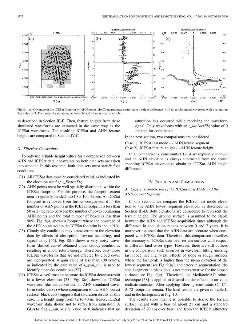
Fig. 8. (a) Coverage of the ICESat footprint by AHN points. (b) Cloud presence resulting in a height difference ≥ 10 m. (c) Saturated waveform with a saturationflag value of 3. The range of saturation, between 39 and 45 m, is clearly visible.

as described in Section III-E. Then, feature heights from thesesimulated waveforms are extracted in the same way as theICESat waveforms. The resulting ICESat and AHN featureheights are compared in Section IV-C.

G. Filtering Constraints

To only use reliable height values for a comparison betweenAHN and ICESat data, constraints on both data sets are takeninto account. In this research, both data sets must satisfy fourconditions.

C1) All ICESat data must be considered valid, as indicated bythe elevation use flag i_ElvuseFlg.

C2) AHN points must be well spatially distributed within theICESat footprint. For this purpose, the footprint extentarea is regularly divided into 10 × 10 m boxes. An ICESatfootprint is removed from further comparison if 1) thenumber of AHN points in the ICESat footprint is less than50 or 2) the ratio between the number of boxes containingAHN points and the total number of boxes is less than90%. Fig. 8(a) shows a footprint where the coverage ofthe AHN points within the ICESat footprint is about 91%.

C3) Cloudy sky conditions may cause errors in the elevationdata by effects of absorption, forward scattering, andsignal delay [56]. Fig. 8(b) shows a very noisy wave-form (dashed curve) obtained under cloudy conditions,resulting in a low return energy. Therefore, only thoseICESat waveforms that are not effected by cloud coverare incorporated. A gain value of less than 100 counts,as indicated by the gain value of i_gval_rcv, is used toidentify clear sky conditions [57].

C4) ICESat waveforms that saturate the ICESat detector resultin a lower elevation [25]. Fig. 8(c) shows an ICESatwaveform (dashed curve) and an AHN simulated wave-form (solid curve) where comparison to the AHN lowestsurface (black dots) suggests that saturation results, in thiscase, in a height jump from 42 to 40 m. Hence, ICESatwaveform data should not to suffer from saturation. AGLA14 flag i_satCorrFlg value of 0 indicates that no

saturation has occurred while receiving the waveformsignal. Only waveforms with an i_satCorrFlg value of 0are kept for comparison.

In the next section, two comparisons are considered.

Case 1) ICESat last mode ↔ AHN lowest segment.Case 2) ICESat feature height ↔ AHN feature height.

In all comparisons, constraints C1–C4 are explicitly applied,and an AHN elevation is always subtracted from the corre-sponding ICESat elevation to obtain an ICESat–AHN heightdifference.

IV. RESULTS AND COMPARISON

A. Case 1: Comparison of the ICESat Last Mode and theAHN Lowest Segment

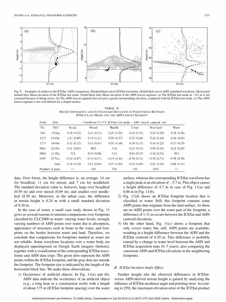
In this section, we compare the ICESat last mode eleva-tion to the AHN lowest segment elevation, as described inSection III-D. Both elevations are considered to represent theterrain height. The ground surface is assumed to be stablebetween the AHN and ICESat acquisition times although thedifference in acquisition ranges between 0 and 7 years. It ismoreover assumed that the AHN data are accurate when com-pared with ICESat data. Therefore, this comparison describesthe accuracy of ICESat data over terrain surface with respectto different land cover types. However, there are still outliersin the comparison, such as errors in waveform fitting [missinglast mode; see Fig. 9(a)], effects of slope or rough surfaceswhere the last peak is higher than the mean elevation of thelowest segment [see Fig. 9(b)], and errors in segmentation [thesmall segment in black dots is not representative for the slopedsurface; see Fig. 9(c)]. Therefore, the Median/MAD robusttechnique [58] is applied to discard outlier effects to arrive atrealistic statistics. After applying filtering constraints C1–C4,3172 footprints remain. The final results are given in Table IIand in the histograms in Fig. 10.

The results show that it is possible to derive the terrainsurface height with a bias of about 21 cm and a standarddeviation of 20 cm over bare land from the ICESat altimetry



Fig. 9. Examples of outliers in the ICESat–AHN comparison. (Dashed black curve) ICESat waveform. (Solid black curve) AHN simulated waveform. (Horizontaldashed line) Mean elevation of the ICESat last mode. (Solid black line) Mean elevation of the AHN lowest segment. (a) The ICESat last mode at −0.2 m is notextracted because of fitting errors. (b) The AHN lowest segment does not give a good corresponding elevation, compared with the ICESat last mode. (c) The AHNlowest segment is not well defined for a sloped surface.

TABLE IIHEIGHT DIFFERENCE AND ITS STANDARD DEVIATION IN PARENTHESIS BETWEEN

ICESAT LAST MODE AND THE AHN LOWEST SEGMENT

data. Over forest, the height difference is, on average, 14 cmfor broadleaf, 11 cm for mixed, and 7 cm for needleleaf.The standard deviation value is, however, large over broadleaf(0.59 m) and over mixed (0.69 m), and smaller over needle-leaf (0.30 m). Moreover, in the urban case, the differencein terrain height is 0.24 m with a small standard deviationof 0.28 m.

In the case of water, a small case study shown in Fig. 11gives us several reasons to mistrust comparisons over footprintsclassified by CLC2000 as water: varying water levels, stronglyvarying numbers of AHN points over water due to absorption,appearance of structures such as boats in the water, and foot-prints on the border between water and land. Therefore, weconclude that comparisons for footprints marked as water arenot reliable. Some waveform locations over a water body aredisplayed superimposed on Google Earth imagery (bottom),together with a visualization of the corresponding ICESat wave-forms and AHN data (top). The green dots represent the AHNpoints within the ICESat footprint, and the gray dots are outsidethe footprint. The footprint size is indicated by the length of thehorizontal black line. We make three observations.

1) Occurrence of artificial objects: In Fig. 11(a) and (b),AHN data indicate the occurrence of an artificial object(e.g., a long boat or a construction work) with a lengthof about 175 m (ICESat footprint spacing) over the water

surface, whereas the corresponding ICESat waveform hasa single peak at an elevation of −5.7 m. This object causesa height difference of 4.7 m in case of Fig. 11(a) and0.86 m in Fig. 11(b).

2) Fig. 11(d) shows an ICESat footprint location that isclassified as water. Still, this footprint contains someAHN points that originate from the land surface. As thereare no AHN points over the water part of the footprint, adifference of 1.31 m occurs between the ICESat and AHNcentroid elevations.

3) On the other hand, Fig. 11(c) shows a footprint thatonly covers water, but, still, AHN points are available,resulting in a height difference between the AHN and theICESat centroid of 0.29 m. This difference is probablycaused by a change in water level between the AHN andICESat acquisition time (0–7 years), also comparing theconsistent AHN and ICESat elevations in the neighboringfootprints.

B. ICESat Incident Angle Effect

Further insight into the observed differences in ICESat-versus AHN-derived terrain height is gained by analyzing theinfluence of ICESat incidence angle and pointing error. Accord-ing to [59], the maximum elevation error of the ICESat product



Fig. 10. Histograms of height differences obtained after applying conditions C1–C4 over (a) broadleaf, (b) mixed, (c) needleleaf, (d) urban, and (e) bare land.Median and standard deviation values have been estimated by the Median/MAD robust statistics [58].

Fig. 11. (Top) Water waveforms with (top right) the number of AHN points within (bottom) the ICESat footprints displayed, together with the Google Earthimage. (Horizontal black line) Last mode height. (Horizontal red line) Mean height of AHN ground points. (Green dots) AHN points located inside the ICESatfootprint. (Gray dots) AHN points outside the ICESat footprint.

is equal to about 7.5 cm/1◦ incident angle with a laser pointingerror of 1.5 arcsec. To limit the impact of incident angle onelevation errors to an effect of maximally a few centimeters,footprints were removed if the ICESat incident angle is largerthan 1◦. By using the AHN data, the ICESat incident angle isobtained from a combination of the ICESat laser pointing angleand the AHN surface slope. The AHN surface slope is obtainedby fitting a plane to the AHN lowest segment data within thefootprint.

In comparison to the previous results, the results show thatthe observed differences in terrain height are strongly changedin forested areas and slightly improved in bare land and ur-ban areas. Over forested areas, the average difference slightlyincreases, i.e., by 13 cm over mixed forest and 5 cm overboth needleleaf and broadleaf forests. The standard deviationis significantly reduced from a maximum of 69 cm (overmixed) to a maximum of 25 cm (over broadleaf). Moreover,over urban and bare land areas, only the standard deviationis reduced by 1–5 cm. The price to pay for the improvementin the statistics is that 873 pairs were removed from a totalof 3172 pairs. Although this analysis was performed overrelatively flat terrain, it demonstrates that the ICESat inci-

dence angle has an impact on the accuracy of the terrainheight.

C. Case 2: Comparison Between the ICESat- andAHN-Derived Feature Heights

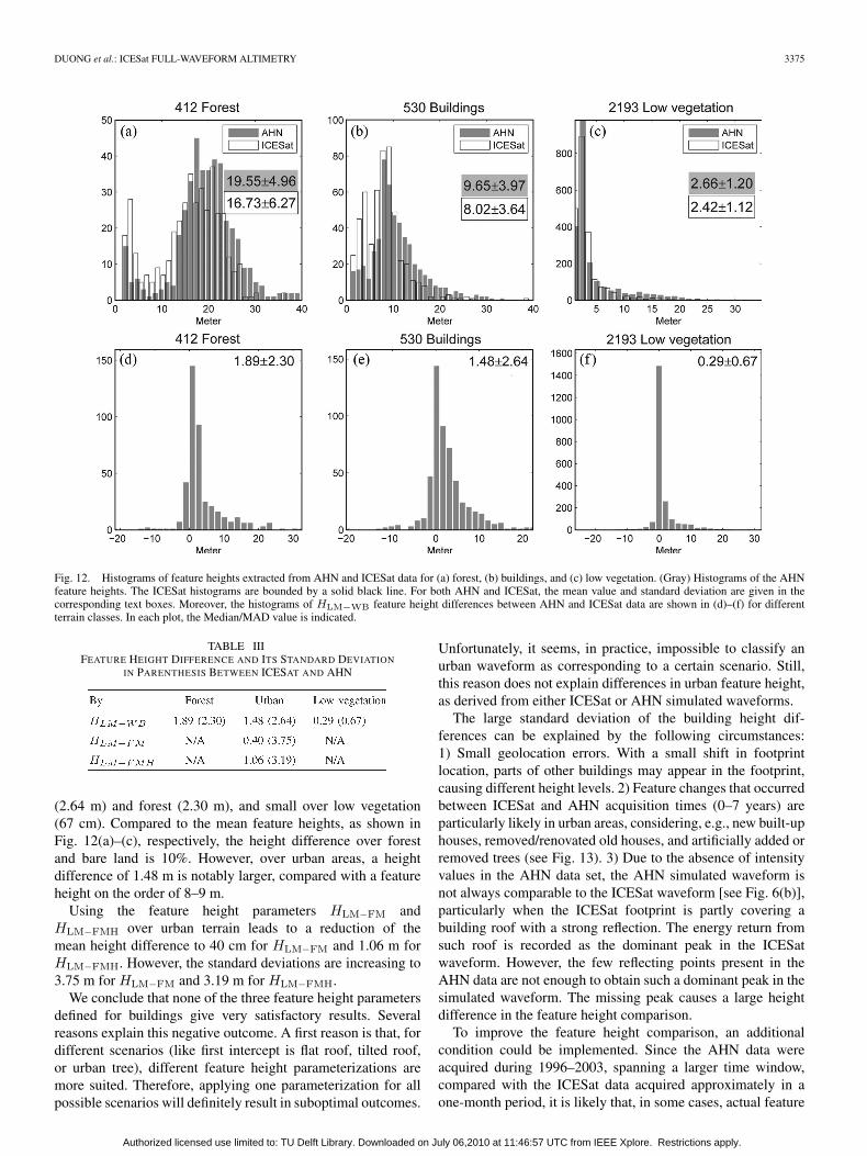
In this section, after applying filtering constraints C1–C4,3172 feature heights derived from ICESat waveforms andAHN simulated waveforms, as defined in Section III-F, arecompared. Histograms of forest, building, and low vegetationheights using parameter HLM−WB are shown in Fig. 12(a)–(c),respectively. On average, the feature height is about 17–20 mover forest, 8–9 m over buildings, and almost 3 m over lowvegetation.

Table III shows height differences with respect to forest,buildings, and low vegetation in terms of feature height param-eter HLM−WB. Moreover, over urban areas, two other featureheight parameters HLM−FM and HLM−FMH were also deter-mined. According to the feature height HLM−WB, the heightdifference between the ICESat data and AHN data is equalto 1.89 m over forest, 1.48 m over buildings, and 29 cm overlow vegetation. The standard deviation is larger over buildings



Fig. 12. Histograms of feature heights extracted from AHN and ICESat data for (a) forest, (b) buildings, and (c) low vegetation. (Gray) Histograms of the AHNfeature heights. The ICESat histograms are bounded by a solid black line. For both AHN and ICESat, the mean value and standard deviation are given in thecorresponding text boxes. Moreover, the histograms of HLM−WB feature height differences between AHN and ICESat data are shown in (d)–(f) for differentterrain classes. In each plot, the Median/MAD value is indicated.

TABLE IIIFEATURE HEIGHT DIFFERENCE AND ITS STANDARD DEVIATION

IN PARENTHESIS BETWEEN ICESAT AND AHN

(2.64 m) and forest (2.30 m), and small over low vegetation(67 cm). Compared to the mean feature heights, as shown inFig. 12(a)–(c), respectively, the height difference over forestand bare land is 10%. However, over urban areas, a heightdifference of 1.48 m is notably larger, compared with a featureheight on the order of 8–9 m.

Using the feature height parameters HLM−FM andHLM−FMH over urban terrain leads to a reduction of themean height difference to 40 cm for HLM−FM and 1.06 m forHLM−FMH. However, the standard deviations are increasing to3.75 m for HLM−FM and 3.19 m for HLM−FMH.

We conclude that none of the three feature height parametersdefined for buildings give very satisfactory results. Severalreasons explain this negative outcome. A first reason is that, fordifferent scenarios (like first intercept is flat roof, tilted roof,or urban tree), different feature height parameterizations aremore suited. Therefore, applying one parameterization for allpossible scenarios will definitely result in suboptimal outcomes.

Unfortunately, it seems, in practice, impossible to classify anurban waveform as corresponding to a certain scenario. Still,this reason does not explain differences in urban feature height,as derived from either ICESat or AHN simulated waveforms.

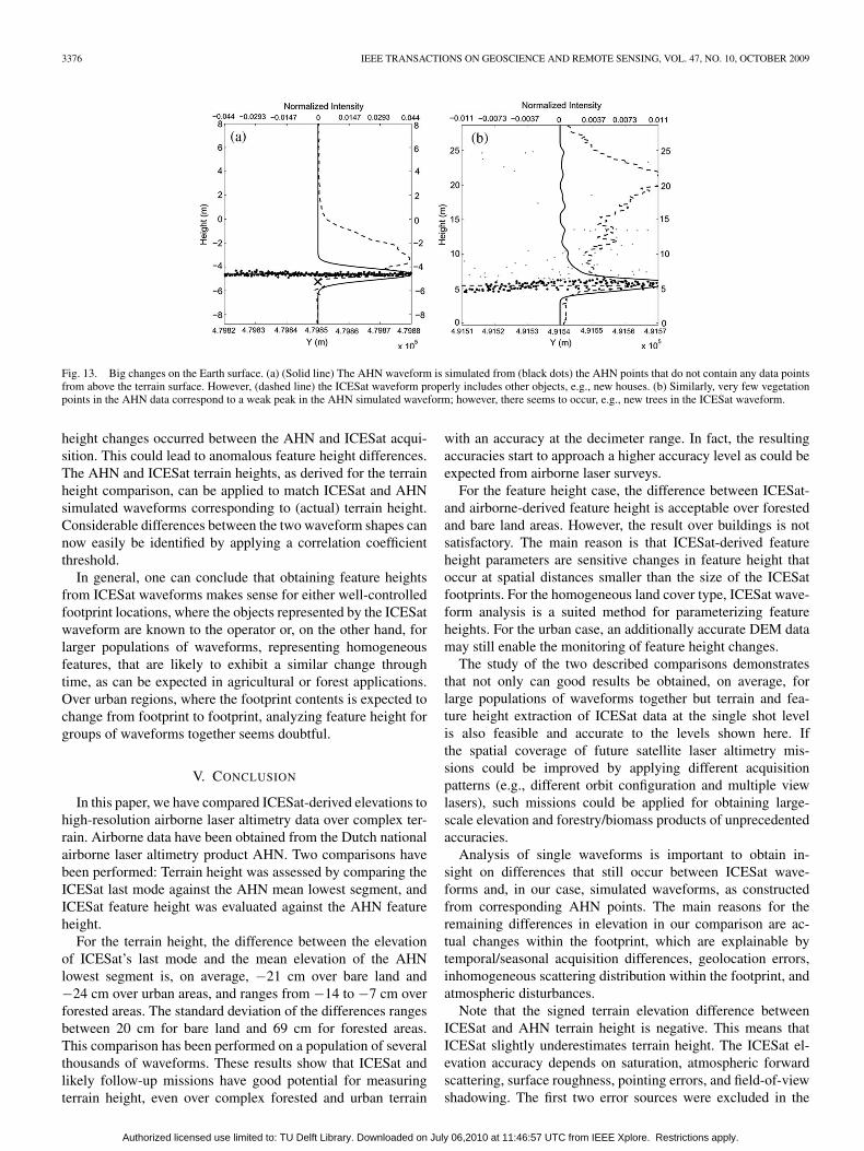
The large standard deviation of the building height dif-ferences can be explained by the following circumstances:1) Small geolocation errors. With a small shift in footprintlocation, parts of other buildings may appear in the footprint,causing different height levels. 2) Feature changes that occurredbetween ICESat and AHN acquisition times (0–7 years) areparticularly likely in urban areas, considering, e.g., new built-uphouses, removed/renovated old houses, and artificially added orremoved trees (see Fig. 13). 3) Due to the absence of intensityvalues in the AHN data set, the AHN simulated waveform isnot always comparable to the ICESat waveform [see Fig. 6(b)],particularly when the ICESat footprint is partly covering abuilding roof with a strong reflection. The energy return fromsuch roof is recorded as the dominant peak in the ICESatwaveform. However, the few reflecting points present in theAHN data are not enough to obtain such a dominant peak in thesimulated waveform. The missing peak causes a large heightdifference in the feature height comparison.

To improve the feature height comparison, an additionalcondition could be implemented. Since the AHN data wereacquired during 1996–2003, spanning a larger time window,compared with the ICESat data acquired approximately in aone-month period, it is likely that, in some cases, actual feature



Fig. 13. Big changes on the Earth surface. (a) (Solid line) The AHN waveform is simulated from (black dots) the AHN points that do not contain any data pointsfrom above the terrain surface. However, (dashed line) the ICESat waveform properly includes other objects, e.g., new houses. (b) Similarly, very few vegetationpoints in the AHN data correspond to a weak peak in the AHN simulated waveform; however, there seems to occur, e.g., new trees in the ICESat waveform.

height changes occurred between the AHN and ICESat acqui-sition. This could lead to anomalous feature height differences.The AHN and ICESat terrain heights, as derived for the terrainheight comparison, can be applied to match ICESat and AHNsimulated waveforms corresponding to (actual) terrain height.Considerable differences between the two waveform shapes cannow easily be identified by applying a correlation coefficientthreshold.

In general, one can conclude that obtaining feature heightsfrom ICESat waveforms makes sense for either well-controlledfootprint locations, where the objects represented by the ICESatwaveform are known to the operator or, on the other hand, forlarger populations of waveforms, representing homogeneousfeatures, that are likely to exhibit a similar change throughtime, as can be expected in agricultural or forest applications.Over urban regions, where the footprint contents is expected tochange from footprint to footprint, analyzing feature height forgroups of waveforms together seems doubtful.

V. CONCLUSION

In this paper, we have compared ICESat-derived elevations tohigh-resolution airborne laser altimetry data over complex ter-rain. Airborne data have been obtained from the Dutch nationalairborne laser altimetry product AHN. Two comparisons havebeen performed: Terrain height was assessed by comparing theICESat last mode against the AHN mean lowest segment, andICESat feature height was evaluated against the AHN featureheight.

For the terrain height, the difference between the elevationof ICESat’s last mode and the mean elevation of the AHNlowest segment is, on average, −21 cm over bare land and−24 cm over urban areas, and ranges from −14 to −7 cm overforested areas. The standard deviation of the differences rangesbetween 20 cm for bare land and 69 cm for forested areas.This comparison has been performed on a population of severalthousands of waveforms. These results show that ICESat andlikely follow-up missions have good potential for measuringterrain height, even over complex forested and urban terrain

with an accuracy at the decimeter range. In fact, the resultingaccuracies start to approach a higher accuracy level as could beexpected from airborne laser surveys.

For the feature height case, the difference between ICESat-and airborne-derived feature height is acceptable over forestedand bare land areas. However, the result over buildings is notsatisfactory. The main reason is that ICESat-derived featureheight parameters are sensitive changes in feature height thatoccur at spatial distances smaller than the size of the ICESatfootprints. For the homogeneous land cover type, ICESat wave-form analysis is a suited method for parameterizing featureheights. For the urban case, an additionally accurate DEM datamay still enable the monitoring of feature height changes.

The study of the two described comparisons demonstratesthat not only can good results be obtained, on average, forlarge populations of waveforms together but terrain and fea-ture height extraction of ICESat data at the single shot levelis also feasible and accurate to the levels shown here. Ifthe spatial coverage of future satellite laser altimetry mis-sions could be improved by applying different acquisitionpatterns (e.g., different orbit configuration and multiple viewlasers), such missions could be applied for obtaining large-scale elevation and forestry/biomass products of unprecedentedaccuracies.

Analysis of single waveforms is important to obtain in-sight on differences that still occur between ICESat wave-forms and, in our case, simulated waveforms, as constructedfrom corresponding AHN points. The main reasons for theremaining differences in elevation in our comparison are ac-tual changes within the footprint, which are explainable bytemporal/seasonal acquisition differences, geolocation errors,inhomogeneous scattering distribution within the footprint, andatmospheric disturbances.

Note that the signed terrain elevation difference betweenICESat and AHN terrain height is negative. This means thatICESat slightly underestimates terrain height. The ICESat el-evation accuracy depends on saturation, atmospheric forwardscattering, surface roughness, pointing errors, and field-of-viewshadowing. The first two error sources were excluded in the



comparison based on quality flags provided in the GLAS prod-uct. The third and fourth error sources have been discussed inthis paper. However, the last one, i.e., field-of-view shadowing,which is significant in campaign L2a data, is not analyzed yet.This factor causes distortion of the laser power distributionwithin the footprint, resulting in clipped/skewed waveformshapes. As a consequence, ICESat elevations can be too lowby several centimeters, with a bias magnitude correlated withthe footprint size and laser energy level [59]. This error sourcecould be the remaining problem for underestimated terrainheights and, therefore, needs to be investigated and quantifiedin further studies. Finally, almost time-coincident data fromairborne AHN2 and recent ICESat campaigns is becomingavailable. Repeating this analysis on these new data sets willenable obtaining better insight into error sources in ICESatheight underestimation and terrain/feature height differencesbetween ICESat and AHN data.

ACKNOWLEDGMENT

The authors would like to thank the National Snow andIce Data Center; G. Hazeu from Wageningen University,Wageningen, The Netherlands; and the European EnvironmentAgency for their guidelines and data distribution.

REFERENCES

[1] H. J. Zwally, B. Schutz, W. Abdalati, J. Abshire, C. Bentley, A. Brenner,J. Bufton, J. Dezio, D. Hancock, D. Harding, T. Herring, B. Minster,K. Quinn, S. Palm, J. Spinhirne, and R. Thomas, “ICESats laser mea-surements of polar ice, atmosphere, ocean, and land,” J. Geod., vol. 34,no. 3/4, pp. 405–445, Oct./Nov. 2002.

[2] A. C. Brenner, H. J. Zwally, C. R. Bentley, B. M. Csatho, D. J. Harding,M. A. Hofton, J. B. Minster, L. A. Roberts, J. L. Saba, R. H. Thomas,and D. Yi, “Geoscience laser altimeter system algorithm theoretical basisdocument: Derivation of range and range distributions from laser pulsewaveform analysis,” Algorithm Theoretical Basis Documents (ATBD),2003. [Online]. Available: http://www.csr.utexas.edu/glas/atbd.html

[3] “Frequently asked question,” ICESat/GLAS Data at NSIDC, 2005.[Online]. Available. http://nsidc.org/data/icesat/faq.html

[4] M. Lefsky, D. Harding, M. Keller, W. Cohen, C. Carabajal, F. Espirito-Santo, M. Hunter, and R. Oliveira, “Estimates of forest canopy height andabove ground biomass using ICESat,” Geophys. Res. Lett., vol. 32, no. 22,pp. L22 S02-1–L22 S02-4, Nov. 2005. DOI:10.1029/2005GL023971.

[5] M. A. Lefsky, W. B. Cohen, D. J. Harding, G. G. Parker, S. A. Acker,and S. T. Gower, “Lidar remote sensing of above-ground biomass in threebiomes,” Glob. Ecol. Biogeogr., vol. 11, no. 5, pp. 393–399, Oct. 2002.

[6] J. Boudreau, R. F. Nelson, H. A. Margolis, A. Beaudoin, L. Guindon,and D. S. Kimes, “Regional above ground forest biomass using airborneand spaceborne lidar in Québec,” Remote Sens. Environ., vol. 112, no. 10,pp. 3876–3890, Oct. 2008.

[7] D. J. Harding and C. C. Carabajal, “ICESat waveform measurementsof within-footprint topographic relief and vegetation vertical structure,”Geophys. Res. Lett., vol. 32, no. 21, pp. L21 810.1–L21 810.4, Oct. 2005.DOI:10.1029/2005GL023471.

[8] G. Sun, K. Ranson, D. Kimes, J. Blair, and K. Kovacs, “Forest verticalstructure from GLAS: An evaluation using LVIS and SRTM data,” RemoteSens. Environ., vol. 112, no. 1, pp. 107–117, Jan. 2008.

[9] J. A. B. Rosette, P. R. J. North, and J. C. Suárez, “Vegetation heightestimates for a mixed temperate forest using satellite laser altimetry,” Int.J. Remote Sens., vol. 29, no. 5, pp. 1475–1493, Mar. 2008.

[10] K. Ranson, G. Sun, K. Kovacs, and V. Kharuk, “Landcover attributesfrom ICESat GLAS data in Central Siberia,” in Proc. IEEE IGARSS,Anchorage, AK, Sep. 20–24, 2004, vol. 2, pp. 753–756.

[11] V. H. Duong, R. Lindenbergh, N. Pfeifer, and G. Vosselman, “Single andtwo epoch analysis of ICESat full waveform data over forested areas,” Int.J. Remote Sens., vol. 29, no. 5, pp. 1453–1473, Mar. 2008.

[12] C. A. Shuman, H. J. Zwally, B. E. Schutz, A. C. Brenner, J. P. DiMarzio,V. P. Suchdeo, and H. A. Fricker, “ICESat Antarctic elevation data:Preliminary precision and accuracy assessment,” Geophys. Res. Lett.,vol. 33, no. 7, p. L07 501, Apr. 2006. DOI:10.1029/2005GL025227.

[13] T. Yamanokuchi, K. Doi, and K. Shibuya, “Combined use of InSAR andICESat/GLAS data for high accuracy DEM generation on Antarctica,” inProc. IEEE IGARSS, 2007, pp. 1229–1231.

[14] J. Wahr, D. Wingham, and C. Bentley, “A method of combining ICESatand GRACE satellite data to constrain Antarctic mass balance,” J. Geo-phys. Res., vol. 105, no. B7, pp. 16 279–16 294, 2000.

[15] D. C. Slobbe, R. C. Lindenbergh, and P. Ditmar, “Estimation of volumechange rates of Greenland’s ice sheet from ICESat data using overlappingfootprints,” Remote Sens. Environ., vol. 112, no. 12, pp. 4204–4213,Dec. 2008.

[16] R. Bindschadler, H. Choi, C. Shuman, and T. Markus, “Detecting andmeasuring new snow accumulation on ice sheets by satellite remotesensing,” Remote Sens. Environ., vol. 98, no. 4, pp. 388–402, Oct. 2005.

[17] H. J. Zwally, D. Yi, R. Kwok, and Y. Zhao, “ICESat measurementsof sea ice freeboard and estimates of sea ice thickness in the wed-dell sea,” J. Geophys. Res., vol. 113, no. C2, p. C02 S15, Feb. 2008.DOI:10.1029/2007JC004284.

[18] J. Bamber and J. L. Gomez-Dans, “The accuracy of digital elevationmodels of the Antarctic continent,” Earth Planet. Sci. Lett., vol. 237,no. 3/4, pp. 516–523, Sep. 2005.

[19] C. C. Carabajal and D. J. Harding, “ICESat validation of SRTMC-band digital elevation models,” Geophys. Res. Lett., vol. 32, no. 22,pp. L22 S01.1–L22 S01.5, Nov. 2005.

[20] C. C. Carabajal and D. J. Harding, “SRTM C-band and ICESat laseraltimetry elevation comparisons as a function of tree cover and relief,”Photogramm. Eng. Remote Sens., vol. 72, no. 3, pp. 287–298, Mar. 2006.

[21] K. J. Bhang, F. W. Schwartz, and A. Braun, “Verification of the verticalerror in C-band SRTM DEM using ICESat and Landsat-7, Otter TailCounty, MN,” IEEE Trans. Geosci. Remote Sens., vol. 46, no. 1, pp. 36–44, Jan. 2007.

[22] N. T. Kurtz, T. Markus, D. J. Cavalieri, W. Krabill, J. G. Sonntag, andJ. Miller, “Comparison of ICESat data with airborne laser altimeter mea-surements over Arctic sea ice,” IEEE Trans. Geosci. Remote Sens., vol. 46,no. 7, pp. 1913–1924, Jul. 2008.

[23] C. F. Martin, R. H. Thomas, W. B. Krabill, and S. S. Manizade, “ICESatrange and mounting bias estimation over precisely-surveyed terrain,”Geophys. Res. Lett., vol. 32, no. 21, pp. L21 S07.1–L21 S07.4, Oct. 2005.DOI:10.1029/2005GL023800.

[24] L. A. Magruder, C. E. Webb, T. J. Urban, E. C. Silverberg, andB. E. Schutz, “ICESat altimetry data product verification at whitesands space harbor,” IEEE Trans. Geosci. Remote Sens., vol. 45, no. 1,pp. 147–155, Jan. 2007.

[25] H. A. Fricker, A. Borsa, B. Minster, C. Carabajal, K. Quinn, andB. Bills, “Assessment of ICESat performance at the Salar de Uyuni,Bolivia,” Geophys. Res. Lett., vol. 32, no. 21, p. L21 S06, Sep. 2005.DOI:10.1029/2005GL023423.

[26] D. Atwood, R. Guritz, R. Muskett, C. Lingle, J. Sauber, andJ. Freymueller, “DEM control in Arctic Alaska with ICESat laser altime-try,” IEEE Trans. Geosci. Remote Sens., vol. 45, no. 11, pp. 3710–3720,Nov. 2007.

[27] A. Braun and G. Fotopoulos, “Assessment of SRTM, ICESat, and sur-vey control monument elevations in Canada,” Photogramm. Eng. RemoteSens., vol. 73, no. 12, pp. 1333–1342, 2007.

[28] D. J. Harding, M. A. Lefsky, G. G. Parker, and J. B. Blair, “Laser al-timeter canopy height profiles: Methods and validation for closed-canopy,broadleaf forests,” Remote Sens. Environ., vol. 76, no. 3, pp. 283–297,Jun. 2001.

[29] European Environment Agency, CORINE Land Cover 2000, 2006.[Online]. Available: http://dataservice.eea.eu.int/dataservice/metadetails.asp?id=822

[30] H. J. Rim and B. E. Schutz, “Precision orbit determination (POD),”Algorithm Theoretical Basis Documents (ATBD), 2002. [Online].Available: http://www.csr.utexas.edu/glas/pdf/atbd_pod_10_02.pdf

[31] S. Bae and B. E. Schutz, “Precision attitude determination (PAD),”Algorithm Theoretical Basis Documents (ATBD), 2002. [Online].Available: http://www.csr.utexas.edu/glas/pdf/atbd_pad_10_02.pdf

[32] B. E. Schutz, “Laser footprint location (geolocation) and surface pro-files,” Center Space Res., Univ. Texas, Austin, Austin, TX, 2002.Tech. Rep.

[33] H. Duong, R. Lindenbergh, N. Pfeifer, and G. Vosselman, “Error analysisof icesat waveform processing by investigating overlapping pairs overEurope,” in Proc. IEEE IGARSS, Barcelona, Spain, Jul. 23–27, 2007,pp. 4753–4756.



[34] AHN, Actual Height Model of The Netherlands, 2008. [Online].Available: http://www.ahn.nl/english.php

[35] T. J. Urban, B. E. Schutz, and A. L. Neuenschwander, “A survey of ICESatcoastal altimetry applications: Continental coast, open ccean island, andinland river,” Terr., Atmos. Ocean. Sci., vol. 19, pp. 1–19, 2008.

[36] R. Heerd, E. Kuijlaars, M. Teeuw, and R. ’t Zand, “ProduktspecificatieAHN,” Rijkswaterstaat, Adviesdienst Geo-informatie en ICT , 2000.

[37] RDNAP, “Rijksdriehoeksmeting and normaal amsterdams peil,” DutchGeometric Infrastructure, 2007. [Online]. Available: http://www.rdnap.nl/

[38] V. Perdigão and A. Annovi, “Technical and methodological guidefor updating corine land cover database,” Joint Res. Centre, Eur.Environ. Agency, Copenhagen, Denmark, 1997. [Online]. Available:http://www.ec-gis.org/document.cfm?id=197&db=document

[39] G. Hazeu, “CLC2000 land cover database of The Netherlands: Moni-toring land cover changes between 1986 and 2000,” Green World Res.,Wageningen, The Netherlands, 2003. Alterra, Alterra-rapport 775/CGI-rapport 03-006, Tech. Rep.

[40] NSIDC, Tools for Working With ICESat/GLAS Data, 2006. [Online].Available: http://nsidc.org/data/icesat/tools.html

[41] J. Meeus, Astronomical Algorithms. Richmond, VA: Willmann-Bell,1991.

[42] RNlN, “PCTrans 4.2.3,” Hydrographic Service of the Royal NetherlandsNavy, 2008. [Online]. Available: http://www.hydro.nl/pgS/en/pctrans_en.htm

[43] Hoog/NAP, Nlgeo2004: Geoid Model Over The Netherlands, 2009.[Online]. Available: http://www.rdnap.nl/algemeen/hoogte/geoide.html

[44] EEA, EEA Reference Grids, 2008. [Online]. Available: http://dataservice.eea.europa.eu/dataservice/metadetails.asp?id=760

[45] NSIDC, GLAS Altimetry Data Dictionary, 2008. [Online]. Available:http://nsidc.org/data/docs/daac/glas_altimetry/data_dictionary_rel28.html

[46] H. Duong, N. Pfeifer, and R. Lindenbergh, “Analysis of repeated ICESatfull waveform data: Methodology and leaf-on/leaf-off comparison,” inProc. Workshop 3D Remote Sens. Forestry, 2006, pp. 239–248.

[47] T. Rabbani, F. A. van den Heuvel, and G. Vosselman, “Segmentation ofpoint clouds using smoothness constraint,” in Int. Arch. Photogramm.Remote Sens. Spat. Inf. Sci., Dresden, Germany, Sep. 25–27, 2006,vol. XXXVI, pt. 5, pp. 248–253.

[48] W. Wagner, A. Ullrich, V. Ducic, T. Melzer, and N. Studnicka, “Gaussiandecomposition and calibration of a novel small-footprint full-waveformdigitizing airborne laser scanner,” ISPRS J. Photogramm. Remote Sens.,vol. 60, pp. 100–112, 2006.

[49] J. B. Blair and M. A. Hofton, “Modeling laser altimeter return waveformsover complex vegetation using high-resolution elevation data,” Geophys.Res. Lett., vol. 26, no. 16, pp. 2509–2512, Aug. 1999.

[50] S. Filin and B. Csathó, “An efficient algorithm for the synthesisof laser altimeter waveforms,” BPRC, Columbus, OH, 2002, Tech. Rep.[Online]. Available: http://bprc.osu.edu/glid/Documents/WF_simulator/Waveform_simulator.pdf

[51] J. M. Abshire, J. F. McGarray, L. K. Pacini, J. B. Blair, and G. C. Elman,“Laser altimetry simulator. Version 3.0: User’s guide,” NASA TechnicalMemorandum 104588, 1994. p. 66. [Online]. Available: http://ntrs.nasa.gov/archive/nasa/casi.ntrs.nasa.gov/19940021649_199402 1649.pdf

[52] M. A. Lefsky, W. B. Cohen, G. G. Parker, and D. J. Harding, “Lidarremote sensing for ecosystem studies,” BioScience, vol. 52, no. 1, pp. 19–30, 2002.

[53] M. Hollaus and W. Wagner, “Operational use of airborne laser scanningfor forestry applications in complex mountainous terrain,” in Proc. 9thInt. Symp. High Mountain Remote Sens. Cartography, 2007, pp. 19–26.

[54] K. Kraus and N. Pfeifer, “Determination of terrain models in woodedareas with airborne laser scanning data,” ISPRS J. Photogramm. RemoteSens., vol. 53, no. 4, pp. 193–203, Aug. 1998.

[55] M. A. Lefsky, M. Keller, Y. Panga, P. B. de Camargod, andM. O. Hunter, “Revised method for forest canopy height estimation fromgeoscience laser altimeter system waveforms,” J. Appl. Remote Sens.,vol. 1, p. 013 537, 2007.

[56] T. Herring and K. Quinn, “Atmospheric delay correction to GLASlaseraltimeter ranges,” Sci. Syst. Appl., Inc., Lanham, MD, 1999. GLASAlgorithm Theoretical Basis Document, Ver. 1.0, Tech. Rep.

[57] A. T. Nguyen and T. A. Herring, “Analysis of ICESat data using Kalmanfilter and Kriging to study height changes in East Antarctica,” Geophys.Res. Lett., vol. 32, no. 23, pp. L23 S03.1–L23 S03.4, Dec. 2005.

[58] J. W. Muller, “Possible advantages of a robust evaluation of compar-isons,” J. Res. Nat. Inst. Standards Technol., vol. 105, no. 4, pp. 551–555,Jul./Aug. 2000.

[59] T. Urban, R. Gutierrez, and B. Schutz, “Analysis of ICESat laser altimetryelevations over ocean surfaces: Sea state and cloud effects,” in Proc. IEEEIGARSS, Boston, MA, Jul. 6–11, 2008.

Hieu Duong (S’06–A’08) received the B.E degreein electrical and electronic engineering from Ho ChiMinh City University of Technology, Ho Chi MinhCity, Vietnam, in 1999 and the M.Eng. degree inremote sensing and GIS from the Asian Instituteof Technology, Bangkok, Thailand, in 2003. He iscurrently working toward the Ph.D. degree in opticaland laser remote sensing, and mathematical geodesyand positioning from the Delft University of Tech-nology, Delft, The Netherlands. His thesis topic is“Large Footprint Full Waveform Analysis in Laser

Scanning Data and Applications.”

Roderik Lindenbergh received the M.S. degreein mathematics from the University of Amsterdam,Amsterdam, The Netherlands, in 1994 and the Ph.D.degree in mathematics from Utrecht University,Utrecht, The Netherlands, in 2002.

He was a Scientific Programmer with the Re-search Institute for Applications of Computer Al-gebra, Eindhoven, The Netherlands, in 1995 and aResearch Assistant in computational group theorywith Queen Mary and Westfield College, London,U.K., in 1996. In 2002, he joined the Delft Institute

of Earth Observation and Space Systems, Delft University of Technology,where he is currently an Assistant Professor in the Chair of Optical and LaserRemote Sensing. His recent work includes deformation analysis and qualityaspects of remote sensing and surveying data, with emphasis on the analysis oflaser ranging data from both terrestrial laser scanners and airborne and satelliteplatforms (ICESat) and fusion of integrated water vapor observations from GPSground stations and the MERIS spectrometer.

Norbert Pfeifer received the Dipl.Ing. and Dr.degrees in surveying engineering from the ViennaUniversity of Technology, Vienna, Austria, in 1997and 2002, respectively.

He was an Assistant Professor with the Delft Uni-versity of Technology and a Senior Researcher withthe alp-S, Centre of Natural Hazard Management,Innsbruck, Austria. He is currently a Professor ofphotogrammetry with the Institute of Photogramme-try and Remote Sensing, Vienna University of Tech-nology. His research interests include topographic

and 3-D modeling, laser scanning, and automatic scene reconstruction.Prof. Pfeifer is a member of the International Society of Photogrammetry and

Remote Sensing.

George Vosselman received the M.Sc. degree ingeodetic engineering from the Delft University ofTechnology, Delft, The Netherlands, in 1986 and thePh.D. degree from the University of Bonn, Bonn,Germany, in 1991.

From 1993 to 2004, he was a Professor of pho-togrammetry and remote sensing with the Delft Uni-versity of Technology. Since 2004, he has been aProfessor of geo-information extraction with sensorsystems with the International Institute for Geo-Information Science and Earth Observation (ITC),

Enschede, The Netherlands. Since 2005, he has been the Editor-in-Chief forthe ISPRS Journal of Photogrammetry and Remote Sensing. He has been chairor co-chair of three ISPRS working groups on processing point clouds since2000. His research interests include methods for semiautomated and automatedmapping using imagery and point clouds, and the quality analysis of dataacquired with laser scanners.

Prof. Vosselman was the recipient of the ISPRS Otto von Gruber Award andthe Hansa Luftbild Award.
