paper theicesat-2laser altimetrymission · paper theicesat-2laser altimetrymission planned to...

INV ITEDP A P E R

The ICESat-2 LaserAltimetry MissionPlanned to launch in 2015, ICEsat-2 will measure changes in polar

ice coverage and estimate changes in the Earth’s bio-mass

by measuring vegetation canopy height.

By Waleed Abdalati, H. Jay Zwally, Robert Bindschadler, Bea Csatho,

Sinead Louise Farrell, Helen Amanda Fricker, David Harding, Ronald Kwok,

Michael Lefsky, Thorsten Markus, Alexander Marshak, Thomas Neumann,

Stephen Palm, Bob Schutz, Ben Smith, James Spinhirne, and Charles Webb

ABSTRACT | Satellite and aircraft observations have revealed

that remarkable changes in the Earth’s polar ice cover have

occurred in the last decade. The impacts of these changes,

which include dramatic ice loss from ice sheets and rapid

declines in Arctic sea ice, could be quite large in terms of sea

level rise and global climate. NASA’s Ice, Cloud and Land

Elevation Satellite-2 (ICESat-2), currently planned for launch in

2015, is specifically intended to quantify the amount of change

in ice sheets and sea ice and provide key insights into their

behavior. It will achieve these objectives through the use of

precise laser measurements of surface elevation, building on

the groundbreaking capabilities of its predecessor, the Ice

Cloud and Land Elevation Satellite (ICESat). In particular,

ICESat-2 will measure the temporal and spatial character of

ice sheet elevation change to enable assessment of ice sheet

mass balance and examination of the underlying mechanisms

that control it. The precision of ICESat-2’s elevation measure-

ment will also allow for accurate measurements of sea ice

freeboard height, from which sea ice thickness and its tempo-

ral changes can be estimated. ICESat-2 will provide important

information on other components of the Earth System as

well, most notably large-scale vegetation biomass estimates

through the measurement of vegetation canopy height.

When combined with the original ICESat observations,

ICESat-2 will provide ice change measurements across more

than a 15-year time span. Its significantly improved laser system

will also provide observations with much greater spatial

resolution, temporal resolution, and accuracy than has ever

been possible before.

KEYWORDS | Ice sheets; ICESat-2; laser altimetry; NASA;

satellite; sea ice; vegetation

I . INTRODUCTION

Observations from satellites and aircraft have revealed that

in the last decade, the Earth’s polar cryosphere has

experienced some remarkable changes. The Greenland and

Antarctic ice sheets are losing mass at an increasing rate

[1]–[3]. Fast flowing outlet glaciers and ice streams, which

carry most of the mass flux from the interiors of the vast

Greenland and Antarctic ice sheets toward the ocean, have

Manuscript received May 29, 2009; revised September 23, 2009. Current version

published May 5, 2010. This work was supported by the ICESat-2 Program, NASA, and

the Cryospheric Sciences Program, NASA.

W. Abdalati is with the Earth Science and Observation Center and Department of

Geography, University of Colorado at Boulder, Boulder, CO 80302 USA

(e-mail: [email protected]).

H. J. Zwally, R. Bindschadler, D. Harding, T. Markus, A. Marshak, and T. Neumannare with the Science and Exploration Directorate, NASA Goddard Space Flight Center,

Greenbelt, MD 20771 USA (e-mail: [email protected];

[email protected]; [email protected]; thorsten.markus-1@

nasa.gov; [email protected]; [email protected]).

B. Csatho is with the Department of Geology, University at Buffalo, Buffalo,

NY 14260 USA (e-mail: [email protected]).

S. L. Farrell is with the Cooperative Institute for Climate Studies, University of

Maryland, College Park, MD 20742 USA (e-mail: [email protected]).

H. A. Fricker is with the Scripps Institution of Oceanography, San Diego,

CA 92121 USA (e-mail: [email protected]).

R. Kwok is with the Jet Propulsion Laboratory, California Institute of Technology,

91125 USA (e-mail: [email protected]).

M. Lefsky is with Colorado State University, Fort Collins, Colorado 80125 USA


S. Palm is with Science Systems and Applications Inc., Lanham, MD 20706 USA


B. Schutz and C. Webb are with the Center for Space Research, University of Texas at

Austin, 78712 USA (e-mail: [email protected]; [email protected]).

B. Smith is with the Polar Science Center, University of Washington, Seattle,

WA 98195 USA (e-mail: [email protected]).

J. Spinhirne is with the University of Arizona, Tucson, AZ 85721 USA


Digital Object Identifier: 10.1109/JPROC.2009.2034765

Vol. 98, No. 5, May 2010 | Proceedings of the IEEE 7350018-9219/$26.00 �2010 IEEE

Authorized licensed use limited to: NASA Goddard Space Flight. Downloaded on June 01,2010 at 14:04:00 UTC from IEEE Xplore. Restrictions apply.

accelerated dramatically [4]–[7]. The sea ice that coversthe Arctic Ocean has decreased in areal extent far more

rapidly than climate models have predicted [8] and has

thinned substantially [9], suggesting that a summertime

ice-free Arctic ocean may be imminent. Some of the thick

and ancient ice shelves that fringe the Antarctic Peninsula

have disintegrated, triggering the acceleration of the outlet

glaciers that feed them [10], [11]. These and other

phenomena suggest that the state of balance of the Earth’spolar ice cover is in transition, with much of it in a

substantial negative downturn. Amidst these dramatic

losses, however, some areas have experienced modest ice

growth. Parts of the Greenland and Antarctic ice sheets

have thickened [12]–[14], and on the whole, the Antarctic

sea ice area has increased slightly in the last three decades

[15]. All of these occurrencesVrapid losses, slight gains,

dramatic increases in ice discharge, etc.Vare indicative ofthe dynamic complexity of polar ice.

Though far-removed from the everyday lives of most of

the world’s population, the behavior of ice sheets and sea

ice is of major and direct consequence to society. The

Greenland and Antarctic ice sheets contain enough ice to

raise sea level by about 7 and 60 m, respectively [2]. Sea ice

exhibits a major influence on the Earth’s planetary energy

budget, influencing global weather and climate; and theArctic ice cover is especially sensitive to and a strong driver

of climate change, in large part due to the positive albedo

feedbacks associated with melting ice. Consequently, the

Earth’s polar ice cover is a critical and potentially unstable

component of the Earth system. NASA’s Ice Cloud and

Land Elevation Satellite-2 (ICESat-2) is specifically

intended to quantify the rate of change of ice sheets and

sea ice and provide key insights into the processes that drivethose changes. It will achieve these objectives through

the use of precise laser measurements of surface eleva-

tion, following the pioneeringVthough compromisedVcapabilities demonstrated by its predecessor, the Ice Cloud

and Land Elevation Satellite (ICESat). These laser altimeter

measurements will also provide important information on

other components of the Earth system, in particular,

vegetation biomass through the measurement of vegetationcanopy height.

II . BACKGROUND

On January 12, 2003, NASA launched ICESat (Fig. 1), the

first satellite mission specifically designed to measure

changes of polar ice, as part of NASA’s Earth Observing

System. ICESat combined state-of-the-art laser rangingcapabilities with precise orbit and attitude control and

knowledge to provide very accurate measurements of ice

sheet topography and elevation change at high along-

track spatial resolution. ICESat achieved this by sampling

over �65-m-diameter footprints every �172 m, and has

elevation retrieval precision and accuracy of �2 and

�14 cm per shot, respectively [16]. By observing changes

in ice sheet elevation (dh/dt), it is possible to quantify

the growth and shrinkage of parts of the ice sheets with

great spatial detail, thus enabling an assessment of icesheet mass balance and contributions to sea level. More-

over, because the mechanisms that control ice sheet mass

loss and gainVchanges in accumulation, surface ablation,

and dischargeVpresumably have distinct topographic ex-

pressions, ice sheet elevation changes also provide impor-

tant insights into the processes causing the observed

changes.

The original ICESat mission’s primary instrument isthe Geoscience Laser Altimeter (GLAS), which carries

three 1064 nm Nd-YAG lasers, each of which was expected

to operate continuously for approximately 18 months to

enable a nearly five-year mission [17]. GLAS also includes a

frequency-doubler in the beam path that converted a

portion of the main 1064 nm beam to 532 nm in order to

enable more accurate atmospheric measurements, since

detectors at green wavelengths are more sensitive thanthose in the near infrared (IR). On-orbit anomalies

resulted in the premature failure of the first laser after

37 days of operation and rapid energy decay in the second

laser. In the face of compromised laser life, ICESat

operations were switched in fall 2003 from continuous

measurement to a campaign mode, in which elevation

measurements were made along repeat ground tracks for

three 33-day periods (a subcycle of the more denselyspaced 91-day exact repeat orbit) each year during

northern hemisphere (NH) fall, winter, and spring seasons

(Table 1). This revised strategy was intended to enable the

mission to meet its overall ice sheet change detection

objectives but with less temporal and spatial detail than

would have been achieved with continuous operation.

Later, beginning in 2007, the NH winter campaigns were

Fig. 1. Schematic diagram of ICESat on a transect over the Arctic.

ICESat uses a 1064 nm laser operating at 40 Hz to make measurements

at 172-m intervals over ice, oceans, and land.

Abdalati et al.: The ICESat-2 Laser Altimetry Mission

736 Proceedings of the IEEE | Vol. 98, No. 5, May 2010


dropped to further extend mission life (Table 1). The

revised operations plan and the excellent performance ofICESat’s third laser have enabled a total of 15 33-day

measurement campaigns over a period of 5.5 years. The

ICESat mission is no longer collecting elevation data as

the final GLAS laser ceased firing in October 11, 2009.

Despite its compromised operation, ICESat has dem-

onstrated a remarkable capability not only to assess

changes in ice sheet elevations (e.g., [14], [18], [19], as

shown in Fig. 2, but also to measure sea ice freeboard,from which thickness can be inferred [9], [20]–[23]. It has

also been used to determine vegetation height and

aboveground biomass [24]–[30], and for various other

applications across a wide range of disciplines. In addition,

ICESat has provided new insights into Antarctic subglacial

hydrology through its unanticipated capability to detect

localized surface deformation (subsidence or uplift) in

response to movement of subglacial water beneath up to4 km of ice [31]–[33].

It was these demonstrated capabilities, coupled with

recent observations of dramatic changes in polar ice,

that led the National Research Council’s Earth Science

Decadal Survey to call for an ICESat follow-on mission[34]. ICESat-2 is intended to carry out the measurements

that were successfully begun by ICESat despite its

compromised operating condition. Advances in laser

technology since the design and launch of ICESat are

such that the problems experienced with ICESat’s analog

pulse laser system can readily be addressed with more

reliable laser diodes and more benign operating condi-

tions. In addition, developments in micropulse lasertechnology allow consideration of new low-energy high-

repetition-rate systems to further improve the capabilities

of ICESat-2.

III . ICESat-2 MISSION OBJECTIVES

Like ICESat, ICESat-2 is expected to support multidisci-

plinary applications; however, following from the Decadal

Survey’s recommendation, the main science goals are

specifically targeted at measuring 1) ice sheet changes,

2) sea ice thickness, and 3) vegetation biomass. The ICESat-2

Table 1 Acquisition Dates and Release Numbers for the 13 91-Day ICESat Campaigns Acquired Up to March 2008

Abdalati et al. : The ICESat-2 Laser Altimetry Mission

Vol. 98, No. 5, May 2010 | Proceedings of the IEEE 737


Science Definition Team (SDT) has defined specific science

objectives for the mission in each of these areas.

A. Ice SheetsThe primary objective of ICESat-2 is to quantify polar

ice sheet contributions to sea-level rise and the linkages toclimate conditions. ICESat-2 will accomplish this by

measuring changes in ice sheet elevation for the purposes

of assessing overall ice sheet mass balance and its variation

in time and space in the context of a changing climate.

Understanding the causes of that spatial and temporal

variability is the key to achieving the ultimate goal of

developing predictive models that will reliably estimate

future ice sheet contributions to sea level.To meet these objectives, ICESat-2 must measure ele-

vation changes with an accuracy and resolution sufficient to

isolate surface-driven change (controlled by accumulation

and surface ablation variability) from dynamic imbalances

(caused by accelerating or decelerating ice flow). We assume

that each of these processes has a spatially variable dh/dt

signature. Melt-driven imbalances, which are often under a

meter in height, should lower or raise surfaces in a mannerthat varies slowly over large distances, decreasing from a

maximum at the margin to zero at the equilibrium line

altitude [35]. Also, since surface melt is driven by atmo-

spheric processes, it should not be significantly different

between adjacent areas of fast-moving ice streams and the

slow-moving ice sheet. Dynamic imbalances, which can be

many meters in magnitude, begin and are usually most

extreme near outlet glacier termini, propagate inward withtime, and vary significantly over small scales in transition

regions between ice stream flow and sheet flow [36].

Accumulation and precipitation will presumably have

variable gradients that would most likely be strongest in

the high accumulation zones near the margins and lowest at

the low accumulation regions at the interior, and will affect

elevation change both above and below the equilibrium line.

Quantifying these distinctions is very important for thedevelopment of predictive models that capture both

dynamic and surface processes. Doing so requires detec-

tion of vertical changes at a level that is significantly

smaller than the seasonal amplitude. It also requires the

characterization of change along linear distances at major

ice boundaries, such as the transition regions from slow

sheet flow to fast stream flow or from grounded ice to

floating ice (Fig. 3). These transition areas exhibit a stronginfluence on the evolution of flow. In view of these

considerations, the SDT determined that ICESat-2 must be

capable of resolution of winter/summer elevation changeFig. 2. Changes in ice elevation derived from ICESat repeat-track

analyses for the period October, 2003 through October, 2007.

The ice sheet continues to increase in elevation inland, as it did

in the 1990s, but thinning at the margins has increased significantly,

due to increased summer melting and acceleration of outlet glaciers.

The dotted line shows the 2000-m contour line, and the dashed line

shows the ice sheet equilibrium line.

Fig. 3. Landsat image of the Jakobshavn Ice Stream from 2002.

Black ovals show transition regions from sheet flow to stream flow.

In these areas, knowledge of topographic change along linear transects

is critical for understanding the controls of these transition zones on

ice stream flow. Inset: ICESat-derived digital elevation model of

Greenland (Dimarzio et al., 2007). The white dot indicates the location

of the larger image.




to 2.5 cm at subdrainage basin scales (25 � 25 km2),annually resolved elevation changes of 25 cm/y on outlet

glaciers (100 km2 areas), and annually resolved elevation

changes of 25 cm/y at outlet glacier margins (along linear

distances of 1 km).

B. Sea IceThere is currently no means of directly measuring sea

ice thickness by satellite; however, a useful proxy is to

measure the freeboard height (the height of the surface

above open water) and estimate the ice thickness based on

the density differences between the floating ice, snow, andwater (Fig. 4). This has been demonstrated with ERS-1,

ERS-2, and Envisat radar altimetry [37], [38], and with

improved spatial sampling and coverage using ICESat laser

altimetry [9], [20]). Arctic Ocean sea ice thickness from

two ICESat campaigns are shown in Fig. 5. Achieving this

capability requires very dense and precise along-track

sampling to measure the differences in height between the

ice surface and that of narrow leads directly.Unlike ice sheet elevation change, the primary

measurement driver for sea ice is precision (i.e., consis-

tency of retrievals between adjacent pulses) rather than

accuracy. Because estimating thickness requires scaling

the freeboard measurement by approximately a factor of

ten, small errors in precision can translate to large errors

in sea ice thickness. Furthermore, as snow loading

depresses the sea ice freeboard, it has to be accountedfor in the calculation of ice thickness. Various approaches

to estimate snow depthVincluding the use of a snow

climatology [37], snowfall from meteorological fields [9],

and derived snow fields from passive microwave data

[22]Vhave been used. A recent assessment [9] shows that

the ICESat thickness estimates are within 0.5 m of icethickness estimated from draft measurements from

profiling sonars on submarines and ocean moorings.

Three centimeter precision (in freeboard) is a mini-

mum required capability, which corresponds to an

accuracy of �0.3 m in thickness or an overall uncertainty

of better than 25% of the current annual ice-volume

production of the Arctic Ocean. Measurement at this level

will enable accurate determination of the spatial ranges ofice thickness across the Arctic (3–4 m) and Southern

(2–3 m) Oceans. It will also resolve the seasonal cycles in

growth and melt (peak-to-trough amplitude of �1.0 m).

The thickness distribution of sea ice controls energy and

mass exchanges between the ocean and atmosphere at the

surface, and the fresh water fluxes associated with melting

ice serve as stabilizing elements in the circulation of the

North Atlantic waters. Basin-scale fields of ice thicknessare therefore essential for improvements in our estimates

of the seasonal and interannual variability in regional mass

balance, the freshwater budget of the polar oceans, and the

representation of these processes in regional and climate

models.

C. VegetationOver vegetated surfaces, echo laser waveforms include

returns from the top of the canopy, within the canopy, and

the ground, which makes laser altimetry very well suited to

measuring vegetation height and structure (Fig. 6).

However, there are significant differences in sampling

and orbit requirements for ice and vegetation measure-

ment objectives. As a result, a separate Earth ScienceDecadal Survey mission, Deformation Ecosystem Structure

and Dynamics of Ice (DESDynI), includes a lidar

specifically designed to measure vegetation height, and

from that estimate above-ground biomass, while ICESat-2

mainly focuses on ice. Nevertheless, because of the vertical

distribution of laser return energy from vegetated surfaces,

ICESat-2 is expected to make important contributions to

Fig. 4. Schematic diagram of sea ice showing the relationships

between sea ice thickness ðTIÞ, ice draft ðDÞ, ice freeboard ðFIÞ, total

freeboard ðFÞ, and snow thickness ðTsnÞ. The laser measures to the

top of the ice/snow surface, and freeboard height is determined from

the difference between the reference ocean level (height within a lead)

and the elevation of the ice/snow surface.

Fig. 5. Sea ice thickness for fall 2007 (ON2007) and spring 2008

(FM08) estimated from ICESat-derived freeboard height with the

pole-hole filled in by interpolation and smoothed with a 50-km

Gaussian kernal (Kwok et al., 2009).




the objectives defined by the vegetation and ecosystem

structure science community, specifically an assessment of

forest biomass through the measurement of canopy height

(Fig. 7). Results from the ICESat mission [25] suggest that

extending the ICESat capability to a 91-day continuous

measurement could make ICESat-2 capable of producing a

vegetation height surface with 3-m accuracy at 1-km spatial

resolution, assuming that off-nadir pointing can be used toincrease the spatial distribution of observations over

terrestrial surfaces.

This sampling, combined with a smaller footprint of

50 m or less, would allow characterization of vegetation at a

higher spatial resolution than ICESat, which is expected to

provide a new set of global ecosystem applications. These

include mapping forest productivity by tracking the growth

of individual forest stands, observations of tree phenology,

forest disease, and pest outbreaks through associated

changes in canopy structure, and the mapping of forestheight and aboveground biomass at a scale that approaches

one that is appropriate for forest carbon management. Such

Fig. 6. Depiction of the illumination of trees by an ICESat or ICESat-2 laser spot (left) and the corresponding waveform (right) (from [24]).

The waveform shows a clear ground return that is spread by the slope of the ground, the top of the canopy, and returns from within the

canopy that are indicative of structure within the crown.

Fig. 7. Global estimates of mean canopy height derived from ICESat. The capability of retrieving tree height with ICESat-2 will contribute

to the large-scale biomass assessments.




improvements would enable the global ecosystem commu-nity to further constrain the sources and sinks of carbon at

regional to continental scales.

D. Other ApplicationsSatellite laser altimetry provides additional information

on a wide range of other Earth surface processes and

characteristics, such as mountain glaciers and ice caps

[39]–[42], river and lake height [43], [44], ocean tides [45],[46], land surface topography [47], coastal ocean height

[44], the geoid and marine gravity field at high latitudes

[48], [49], etc. In addition, the atmospheric measurement

capability of ICESat-2, even at near-IR wavelengths, will

enable global measurements of cloud and aerosol structure

to extend the record of these observations beyond those

provided by the lasers onboard ICESat [50] and

CALIPSO [51]. This demonstrated range of capabilitiesindicates that ICESat-2 will make important multidisci-

plinary science contributions; however, it is the ice sheet,

sea ice, and vegetation science objectives that drive the

mission implementation strategies.

IV. ICESat-2 MISSION CONSIDERATIONS

A. Technical ConsiderationsThe accurate measurement of ice sheet change requires

that elevation measurements be made repeatedly over a

time interval that is frequent enough to observe the

temporal character of changes in a meaningful way. At the

same time, the spatial sampling must be sufficiently dense

that change can be characterized on the scales at which

they vary. To achieve this, the original ICESat mission wasplaced in a 91-day exact repeat orbit with a 94� inclination

at 600 km altitude and used repeat observations of

prescribed ground tracks for change determination.

ICESat-2 is planned to fly in a similar orbit that repeats

these ground tracks, in part because this orbit optimizes

the tradeoff between temporal and spatial sampling,

providing maximum coverage density while allowing

observation opportunities of each ground track once everythree months.

Spatial sampling density is of most significance on the

outlet glaciers at the ice sheet margins. The spacing

between ascending tracks for this orbit is shown as a

function of latitude in Table 2. For latitudes greater than

70�, the spacing between ascending and descending tracks

is less than 5 km. (On average, the spacing between

ascending and descending tracks will be about half of whatis reported in Table 2.) This spacing, combined with the

fact that most glaciers are not oriented parallel to ascending

or descending tracks, means the large majority of outlet

glaciers in Antarctica and Greenland will be observed,

many on multiple passes, in the 91-day orbit. Even with the

compromised 33-day orbits of ICESat, important observa-

tions of outlet glacier changes have been made [18]. With

the threefold increase in sampling density with ICESat-2

that will be achieved by repeating the 91-day orbit, thiscapability will be improved upon significantly. In addition,

repeating the ICESat orbit enables direct repeat-track

comparisons between ICESat and ICESat-2, which facil-

itates linking the two missions for an extended change

assessment that will span more than 15 years.

Achieving repeat track capability imposes very strin-

gent requirements on pointing and orbit control and

knowledge. Like its predecessor, ICESat-2 is planned tohave the ability to point to reference ground tracks to

within 30 m (1-sigma) in order to minimize the separation

between observations along each repeat pass. Analysis by

the ICESat-2 science definition team [52] indicates that

with the 30-m pointing ability, satisfying the change-

detection requirements means that the location of the spot

on the ground must be known to better than 4.5 m. This

level of knowledge is necessary to minimize the effects ofsurface slope on the elevation change measurement. Also

like ICESat, we plan to control the orbit to within 800 m of

the reference track to maintain pointing levels of less than

0.1�. Larger values introduce an apparent slope effect that

contributes significantly to dh/dt errors. The orbit must

also be known to within 2 cm radial distance to satisfy the

dh/dt measurement accuracy requirements.

B. Physical ConsiderationsIn addition to these technical considerations, there are

physical characteristics of the ice and the atmosphere that

influence measurement accuracy. Most significant among

these are ice surface roughness and forward-scattering of

photons by clouds and blowing snow from a direct

measurement perspective and firn density variability for

the conversion of elevation change to mass balance.

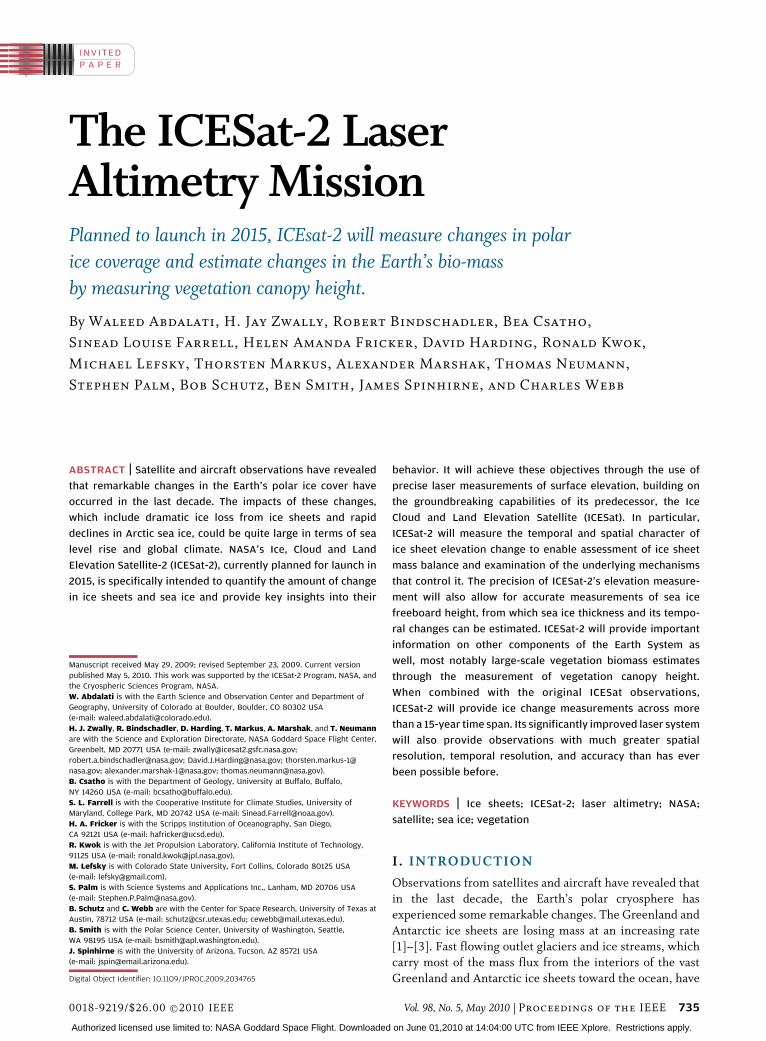
Table 2 Spacing Between Ascending or Descending Ground Tracks in

ICESat’s 91-Day, 94 Inclination, 600 km Altitude Orbit




The horizontal scales of ice sheet roughness vary frommillimeters to kilometers with meteorological processes

driving small-scale variability, while ice flow and topog-

raphy of the underlying bedrock control the large-scale

variability. The scales most significant for altimetry are on

the order of meters to tens of meters for within-footprint

measurement accuracy and meters to hundreds of meters

for accuracy of interpolation between footprints. One way

to minimize noise introduced by surface roughness is byusing small footprints at high along-track sampling rates to

characterize the surface variability. Another is to use larger

footprints to smooth over the roughness elements, which

lowers the sampling rate required to achieve a particular

accuracy. Because laser life is the primary limiting factor

on mission duration and thus science return, strategies

that most sparingly use the finite number of laser shots are

preferable to those that require high sampling rates forconventional analog pulse lasers.

For ICESat-2, the baseline plan has been for approxi-

mately a 50 m footprint size at 50 Hz pulse-repetition

frequency (PRF), which provides laser shots spaced at 140 m

along-track. For the vast majority of the Greenland and

Antarctic ice sheets, 140 m is a reasonable scale over which

the elevation can be interpolated [52]. SDT analyses show

that footprints of this size and spacing should smooth outthe surface roughness characteristics sufficiently, so that

ICESat-2 can achieve the desired measurement accuracy at

this sampling rate [52]. At 50 Hz, the ICESat-2 along-track

sampling would be 20% more dense than that of ICESat.

Previous analyses have shown that forward scattering

of photons in clouds leads to pulse broadening and a range

bias for surface altimetry. This occurs because the path of

photons forward-scattered through clouds from thesatellite to the ground and back to the sensor is not direct

and, if not accounted for, can bias elevation retrievals by

meters [53]. It has been shown [54] that by filtering plus

estimating, the ranging errors from the 532 nm data could

sufficiently correct ICEsat surface elevations to meet all

science requirements. Because atmospheric science is not

an objective of the ICESat-2 mission, a strategy for dealing

with forward scattering is necessary that does not rely ondirect atmospheric measurements from a 532 nm laser.

For actual ICESat data, cloud-clearing based on the

1064 nm ICESat return signal addresses the largest effects,

but a bias of as much as 10 cm or more from clouds and

blowing snow remains. For ICESat-2, a means to bring

forward scattering errors to below the elevation accuracy

requirements is necessary for a 1064 nm altimeter.

Reducing the instrument field of view (FOV) can reducethe forward scattering biases significantly, since more of

the scattered photons are outside the smaller fields of view.

To examine the extent to which reducing the FOV can

mitigate forward scattering effects, the SDT analyzed data

from several areas in Antarctica (Fig. 8) using an estimated

range delay (ERD) from cloud scattering based on ICESat

cloud statistics. The range delay was estimated using Monte

Carlo and analytical radiative transfer calculations using

the best available particle and scattering models for ice

clouds over ice sheets [53], [55]. The analysis was carried

out using accurate cloud data from fall 2003 when the

532 nm channel was operating [52].

We have modeled the approach of reducing the receiver

FOV and applying corrections that could be done with ICEsat1064-nm cloud detection. Results are shown in Table 3 for

one-month averages over the areas shown in Fig. 8. The

estimate of the residual error was based on the analysis of

the relative frequency of optically thin clouds detected by the

532-nm channel but undetected by the 1064-nm channel as a

function of cloud optical depth retrieved from the 532-nm

channel [50]. The error includes those clouds below the level

of detection with the 1064-nm-only cloud channel. Theseanalyses indicate that for fields of view on the order of 100–

160 �rad (60 and 100 m on the ground, respectively), the

effects of forward scattering on 1064 nm analog laser pulses

are reduced to near or within the accuracy requirements.

However, in order to reach these accuracies, a cloud and

blowing snow detection capability similar to that of the

existing ICESat 1064-nm channel would need to be available

for ICESat-2. This in turn would place minimum require-ments on laser energy that are consistent with those required

for altimetry discussed below.

Finally, the primary challenge in converting altimetry

observations of ice sheet elevation change to mass balance

is in the uncertainty in the density of mass lost or gained.

Several models have been developed to account for

elevation changes attributable to firn densification [56],

[57], which have been instrumental in the interpretation ofelevation changes from past and current altimetry missions

(e.g., [1], [58], and [59]). Another aspect of that

Fig. 8. Areas in Antarctica where analysis of field-of-view effects were

examined. The background figure is a shaded-relief digital elevation

model of Antarctica derived from ICESat (Dimarzio et al., 2007). The

gray circle in the middle shows the ‘‘pole-hole’’ area that is not covered

by the 94� inclination of ICESat.




conversion, however, is assessing how much of the

observed elevation changes in the accumulation zones are

dynamically driven and how much are dominated by

surface balance. In the case of the former, the conversion of

elevation change to mass change assumes the density of ice,

while in the case of the latter, the volume lost is assumed to

be the density of firn. Observations and model estimates of

surface balance and flow characteristics provide importantinsights into the relative weighting between the two in

order to reduce uncertainty. More directly, however,

comparisons between mass change estimates derived

from the Gravity Recovery and Climate Experiment

(GRACE) and elevation changes from altimetry enable

estimates of the densities for the volume-to-mass conver-

sions at large spatial scales on the order of 200–500 km,

which has been used to constrain higher resolution ICESatobservations [14], [59]. GRACE has its own limitations,

arising from the large uncertainties related to postglacial

rebound, but the combination of ICESat and GRACE is

improving our understanding of both ice sheet density and

the postglacial rebound. Unfortunately, it is not clear that

ICESat-2 and the successor to GRACE will overlap in the

current implementation plan of the Decadal Survey.

However, the information learned from comparisonsbetween the current ICESat and GRACE missions will be

used to improve densification models and our understand-

ing the dynamic and surface contributions to mass balance.

These in turn will inform our interpretation of elevation-

change signals from ICESat-2.

C. Mission DurationA major consideration for the mission implementation

is maximizing laser life in order to enable a continuously

operating five-year mission. For ice sheets, five years is

the minimum necessary to characterize ice sheet inter-

actions with climate, as it is on the order of the shortest

time scales of surface balance variability [60], [61]. It is

also the absolute minimum time required to examine the

responses of outlet glaciers and ice sheets to major

forcings such as the catastrophic collapse of a floating ice

shelf or retreat of outlet glacier floating tongues.

Responses to these forcings include both the inward

propagation of the marginal perturbation effects, which

can take years [36], and the time required for outlet

glaciers to establish a new quasi-steady-state surface and

velocity profile after such perturbations [62]–[65]. Five

years of observations will not capture the full evolution offorcing and response in most cases, but sustained,

continuous, and detailed observations of this duration or

longer will advance the capabilities of ice sheet and outlet

glacier models that seek to describe ice-climate interac-

tions and the physics associated with responses to major

forcings.

In the case of sea ice, five or more years are also

necessary for developing an understanding of the ocean/atmosphere/sea ice exchanges. It has been shown, for

example, that the behavior of the anomalies of tempera-

ture and salinity in the central Arctic Ocean follows a first-

order linear response to the Arctic Oscillation with a time

constant of five years and a delay of three years [66]. Ice-

climate interactions must be observed through at least a

typical cycle of high-frequency climate processes like the

Arctic Oscillation in order to characterize ice-climateinteractions. Anything shorter will subsample this vari-

ability and will alias the ice-change signal that follows from

such quasi-periodic climate processes.

As the mission proceeds, mapping of forest height

and biomass will be improved as the areas between tracks

are filled in and the spatial density of observations

increases. A longer mission will also (as with the other

application areas) allow a longer period to monitorchange in forest height and aboveground biomass due to

stand growth, changes in forest health, and recovery

from disturbance.

Finally, five years of observation starting in 2015 will

provide a sufficiently long period between the earliest

ICESat measurements and the latest ICESat-2 measure-

ments to quantify more than 15 years of change. Such a

Table 3 Estimated Range-Delay (ERD) Results for Four Different Fields of View in Different Regions of Antarctica (Shown in Fig. 8). The First Row Shows

Analysis of the Average ERD With No Cloud Clearing or Correction With the Effect From Clouds and Blowing Snow Shown Separately. The Second Row Is

an Estimated Residual Error After Cloud Clearing Feasible From Direct 1064 nm Cloud Signals




time span facilitates separation of climatologically signif-icant trends from short-term variability in the combined

ICESat/ICESat-2 time series.

Strategies being adopted to maximize laser life include

maintaining a low PRF to spread a finite number of shots

over a long period and operating at low energy to minimize

the stress on the lasers. There are tradeoffs, however, and

the advantage of implementing these strategies must be

weighed against the need for high energy to penetrate thinand clouds and the need for high PRF to sample surface

variability sufficiently. The tradeoffs between PRF and

footprint size, and their implications on laser life, have been

discussed under Section IV-B, and they suggest that for a

single-beam laser system like GLAS on ICESat, a baseline

configuration with a footprint size of approximately 50 m

and a PRF of 50 Hz (140 m along-track spacing).

Each ICESat laser at intial start-fire operated at app-roximately 70 mJ. For a similar laser system on ICESat-2,

the requirement would be reduced to 50 mJ, assuming a

telescope size of 1-m like ICESat carried. ICESat-2 SDT

analyses show that at these levels, every 10 mJ reduction in

transmit energy corresponds to an average decrease in the

amount of surface returns by 2–4% [52]. However, in

certain regions such as coastal Antarctica and Greenland

and over sea ice, the loss of surface returns can be as muchas 15% per 10 mJ of laser energy. While higher energy

would be preferable, in order to maximize the amount of

surface returns, a reduction to at least 50 mJ is necessary to

reduce stress on the lasers. Current laboratory assessments

of a modified version of the original ICESat engineering test

unit have demonstrated nearly 2.6 billion shots at 50 Hz and

50 mJ with minimal energy loss. At 2 billion shots per laser

and 50 Hz, four lasers operating one at a time should supporta five-year mission. Configurations considered include as

many as six lasers, with the two additional lasers carried

primarily for redundancy, but also in part as recognition of

the importance of long-term measurements. If all six

lasers were to perform at the 2 billion shot level, ICESat-2

could provide more than seven years of measurement at

50 Hz. Additionally, a laser energy of at least 50 mJ will

ensure a sufficient cloud and blowing snow detectioncapability, which is crucial for identifying and filtering

altimetry measurements that have been biased by forward

scattering.

V. MISSION STATUS

The Decadal Survey categorized its recommended mis-

sions into three tiers: near-term, mid-term, and long-term.ICESat-2 is one of four first-tier (near-term) missions

recommended for launch as early as 2010. Currently

planned for launch in the 2015 time frame, ICESat-2 is still

in the early stages of development. However, experiences

with ICESat and associated lessons-learned have provided

important information that inform the design significantly.

These experiences combined with the science require-

ments from the SDT have led to a flow-down from scienceobjectives to measurement requirements to instrument

and mission requirements, as shown in Table 4. With the

mission only recently entering Phase A, which is when the

preliminary design and project plan are developed, a

number of important tradeoffs are under consideration to

provide the optimum science return. Despite this, the

elements of Table 4 present well-understood requirements

that provide a solid design foundation.Fundamental to the success of ICESat-2 is understand-

ing and overcoming the causes of ICESat’s premature laser

failure (laser 1) and rapid energy degradation (laser 2). The

cause of failure for laser 1 was found to be the erosion of

gold conductors in the laser diode array due to excessive

amount of indium solder. This solder combined with the

gold to form nonconducting gold indide, which caused the

diode array to stop functioning [67]. The likely cause ofrapid energy loss in laser 2 is believed to have been a

photodarkening that occurred at and near the laser’s

frequency doubler [68]. In particular, trace levels of

hydrocarbons outgassed from adhesives used in the laser

are believed to have interacted with the 532 nm photons.

These issues will be addressed on ICESat-2 by eliminating

indium from the solder material and possibly pressurizing

the housing to avoid outgassing. The nearly 2.6 billionshots to date on the engineering test unit with these

mitigation strategies implemented indicate that at least

one candidate laser system can achieve five years or more

of continuous measurements at 50 Hz and 50 mJ with four

or more lasers.

The mid-decade launch date, coupled with the fact

ICESat is no longer collecting altimetry data, will lead to a

multiyear gap in satellite laser altimetry measurementsbetween ICESat and ICESat-2. In the intervening period,

NASA is implementing Operation IceBridge, a series of

airborne campaigns in Greenland, Antarctica, and their

surrounding seas, designed to survey high-priority areas

with a range of instrumentation that includes airborne

laser altimetry. IceBridge observations will provide some

continuity of data between missions for these high-priority

targets and collect data in support of model development.1

In addition, the European Space Agency’s satellite

radar altimeter CryoSat-2 is scheduled for launch in early

2010. Cryosat-2 is a three-year mission that is also

intended to measure ice sheet changes and sea ice free-

board height, but it will do so using radar altimetry at up to

250-m along-track resolution based on an interferometric

processing technique [69]. As a radar altimeter, Cryosat-2

will provide coverage under cloudy conditions. On sea ice,the penetration characteristics of radar into snow that may

overlie sea ice make its returns more likely to be from the

interface between the ice and snow, rather than from the

snow surface itself. In other words, it will likely measureFI in Fig. 4, rather than F. Since the presence of snow on

1Details can be found at http://www.espo.nasa.gov/oib/.




sea ice adds uncertainty to the thickness estimate (for

lasers by changing the total column density used to convert

freeboard to thickness, and for radar, by lowering the ice/

snow interface under the weight of the snow), it must be

accounted for in either measurement. Currently, this is

estimated using snow climatology [37], snowfall from

meteorological fields [9], or derived snow fields from

passive microwave data [22]. If there is overlap between

Table 4 General Flowdown From Science Goals to Implementation Requirements




ICESat-2 and Cryosat-2, however, differences in freeboardheight over the same locations will presumably provide a

direct measure of snow height. Also, with ICESat-2’s

smaller laser footprint, it should be able unambiguously

sample smaller leads than Cryosat-2. A comparison be-

tween the two should help quantify the lead size iden-

tifiable by Cryosat-2 and the implications for freeboard

estimates for both measurement approaches.

On ice sheets, Cryosat-2’s all-weather capability willprovide more observations under cloudy conditions that are

often persistent in some of the coastal areas of Greenland

and Antarctica. However, because it carries a Ku-band

radar, variable penetration into firn adds an uncertainty to

the elevation change retrievals that is not inherent in the

laser observations. Moreover, the repeat-track capability of

ICESat-2 will allow change detection along linear tracks,

providing much greater detail in the along-track directionthan can be achieved with the traditional crossover

analysis, as will be done with Cryosat-2.

Though the measurement technologies are very differ-

ent between ICESat/ICESat-2 and Cryosat-2, each is a

valuable complement to the other, and together they will

provide crucial data on ice sheet and sea ice changes over

most of the 2003-2020 time period. The greatest benefits

will be realized if there is significant overlap betweenCryosat-2 and ICESat-2 for a year or more, which will allow

cross-calibration between the two missions.

VI. MISSION CONFIGURATION OPTIONS

Three basic candidate mission configuration options have

been examined for ICESat-2. The simplest employs a single-

beam near-infrared laser approach that would be very

similar to ICESat (Fig. 1). Like ICESat, it would carry

multiple lasers with only one operating at a time. Because it

is not possible to overlay each repeat track exactly on top ofone another, along-track and cross-track offsets in the beam

locations between repeat tracks on the sloped ice sheet

surface can introduce significant errors in the elevation

change calculations. These errors manifest themselves as

Bapparent[ elevation changes between repeat passes due to

the component of surface slope in either the along-track or

the cross-track direction. Along-track slopes can be estimat-

ed from adjacent consecutive measurements, but cross-trackslopes must employ data from multiple passes (Fig. 9).

Correcting for this in repeat-track analyses usually employs a

simultaneous solution of cross-track slope ð�Þ and elevation

change (dh/dt) according to the following formula:

Hðx; �; tÞ ¼ Hðt1Þ þ x tanð�Þ þ tðdh=dtÞ (1)

where H is the surface height at the reference track at time t(with t1 being the time of the first measurement) and x is a

horizontal distance from the reference track.

As a result, for a single-beam configuration, repeat-track

elevation change can only be determined after a sufficient

number of observations has been acquired, in order to solve

(1). At a minimum, this is four observations, but in practice,

analyses of ICESat data have shown that achieving therequired elevation change accuracy requires ten or more. In

coastal regions, where a vast majority of ice loss occurs,

surface signals are not retrieved for approximately half of the

passes, due to extinction under persistent optically thick

atmospheric conditions [70]. Under these circumstances,

approximately five years of measurements are needed on

average before the required change-detection accuracy can

be achieved. Moreover, assessing the variability in dh/dt inthis way requires the assumption that slopes are constant

throughout the mission. This constant-slope assumption is

reasonable for the ice sheet interior, but near the margins,

slopes will likely change considerably throughout the

mission, especially following major change events. Thus

capturing changes in these crucial areas of the ice sheets

requires the simultaneous measurement of cross-track slope

and elevation. This has led the ICESat-2 SDT to recommendthe incorporation of a cross-track measurement capability in

order to enable the direct observation of slope and elevation

and their time-varying changes.

The geometry of any cross-track implementation has

to take into account that the spacecraft may not remain

in the same orientation with respect to its velocity vector

throughout the year. At an inclination of 94�, ICESat-2, like

ICESat, will not be sun-synchronous. To maintain suf-ficient illumination of its solar panels to meet power

requirements, ICESat executes a series of 90� yaw ma-

neuvers twice each year, such that during half the year, the

solar panels are aligned perpendicular to the velocity vector

(referred to as airplane mode) and half the year, they are

aligned parallel to the velocity vector (referred to as

sailboat mode). Cross-track approaches under consider-

ation are those that can accommodate both airplane andsailboat mode.

Fig. 9. Representation of a rising ice sheet surface that is observed by

seven individual ground tracks that are oriented perpendicular to the

page. Each number represents a different observation period, and

the diagonal line passing through that number represents the height of

the sloped surface at the time of observation. Each observation is

offset some distance (x) from the reference track (the black dot at the

intersection of the ‘‘Cross-track’’ and ‘‘HðtÞ’’ axes).




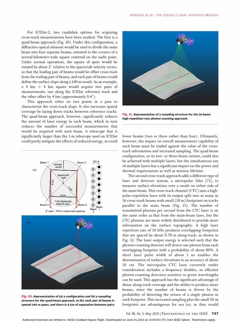
For ICESat-2, two candidate options for acquiringcross-track measurements have been studied. The first is a

quad-beam approach (Fig. 10). Under this configuration, a

diffractive optical element would be used to divide the main

beam into four separate beams, oriented to the corners of a

several-kilometer-wide square centered on the nadir point.

Under normal operations, the square of spots would be

rotated by about 2� relative to the spacecraft velocity vector,

so that the leading pair of beams would be offset cross-trackfrom the trailing pair of beams, and each pair of beams would

define the surface slope along a 140-m swath. As an example,

a 4 km � 4 km square would acquire two pairs of

measurements, one along the ICESat reference track and

the other offset by 4 km (approximately 0.4�).

This approach relies on two points in a pass to

characterize the cross-track slope. It also increases spatial

coverage by laying down tracks between reference tracks.The quad-beam approach, however, significantly reduces

the amount of laser energy in each beam, which in turn

reduces the number of successful measurements that

would be acquired with each beam. A telescope that is

significantly larger than the 1-m telescope used on ICESat

could partly mitigate the effects of reduced energy, as could

fewer beams (two or three rather than four). Ultimately,

however, the impact on overall measurement capability of

each beam must be traded against the value of the cross-

track information and increased sampling. The quad-beam

configuration, or its two- or three-beam variant, could also

be achieved with multiple lasers, but the simultaneous use

of multiple lasers has a significant impact on the power andthermal requirements as well as mission lifetime.

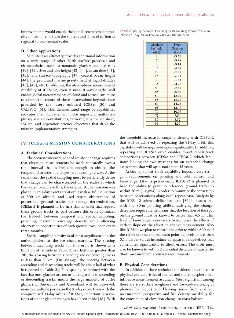
The second cross-track approach adds a different type of

laser and detector system, a micropulse lidar [71], to

measure surface elevations over a swath on either side of

the main beam. This cross-track channel (CTC) uses a high-

pulse-repetition laser with its output split into as many as

16 cross-track beams with small (10 m) footprints on tracks

parallel to the main beam (Fig. 11). The number oftransmitted photons per second from the CTC laser is on

the same order as that from the main-beam laser, but the

CTC photons are more widely distributed to provide more

information on the surface topography. A high laser

repetition rate of 10 kHz produces overlapping footprints

that are spaced by about 0.70 m along-track, as shown in

Fig. 12. The laser output energy is selected such that the

photon-counting detector will detect one photon from eachoverlapping footprint with a probability of about 80%. A

short laser pulse width of about 1 ns enables the

determination of surface elevations to an accuracy of about

10 cm. The micropulse CTC laser currently under

consideration includes a frequency doubler, so efficient

photon-counting detectors sensitive to green wavelengths

can be used. This approach has the significant advantage of

dense along track coverage and the ability to produce morebeams, since the number of beams is driven by the

probability of detecting the return of a single photon in

each footprint. This increased sampling plus the small 10-m

footprints are advantageous for sea ice, as they would

Fig. 10. Representation of (a) a configuration and (b) a sampling

structure for the quad-beam approach. In (b), each pair of beams is

spaced 140 m apart, and there is 4 km of separation between pairs.

Fig. 11. Representation of a sampling structure for the 16-beam

high-repetition-rate photon-counting approach.




enable the detection of smaller leads, which would improve

freeboard measurement accuracy. At green wavelengths,

there is the added complexity of the penetration into the

leads, which will require filtering of subsurface returns. In

the combined micropulse/analog configuration shown in

Fig. 11, any ambiguities can be further resolved through

cross-calibration with a near-IR beam.

The CTC approach also has the potential to improvemeasurements of vegetation canopy heights along each

cross-track beam using algorithms that calculate the along-

track surface elevation profile. Calculation of the surface

profile enables construction of above-surface canopy

height distributions independent of surface slope over

lengths greater than the 10 m footprint size. These canopy

height distributions can also be constructed over various

along-track distances (e.g., 100–500 m) corresponding tothe appropriate decorrelation length scale of the various

vegetation types. The extent to which this approach will

support vegetation and ecosystem science objectives is

currently under investigation.

A fully capable micropulse lidar system can potentially

serve both the primary and cross-track measurement func-

tions, eliminating the need for the analog pulse lidar; however,

the two are most effective as complementary measurements.The analog pulse laser is familiar and has significant heritage,

in terms of both space flight and algorithms. The micropulse

lidar is offers potentially excellent sampling capabilities;

however, it is a novel approach with a limited history. Flying

both lasers simultaneously would provide an important cross-

calibration opportunity that would enable effective merging

the strengths of the two.

VII. SUMMARY AND CONCLUSIONS

The Earth’s ice cover has experienced substantial and

unexpected changes in the last few decades, and satellite

laser altimetry has been demonstrated as a very useful toolfor examining and understanding these changes. Because of

the severely compromised performance of two of its three

lasers, the original ICESat mission never realized its full

potential. ICESat has, however, provided many important

insights into the value of laser altimetry for ice sheet, sea

ice, vegetation, and other measurements, and has provided

a unique initial time series to help assess the state of polar

ice. ICESat-2 will carry this capability forward into thefuture and provide continuous detailed observations of the

polar ice and vegetation with three or more the spatial

coverage of ICESat. In so doing, it will enable scientists to

quantify the seasonal and annual contributions of the ice

sheets to sea level rise, the rate of mass balance changes of

Arctic and Antarctic sea ice, and the amount of global

biomass, with unprecedented accuracy.

In the case of ice sheet changes, ICESat-2 will go beyondthese historic assessments and provide important and

unique insights into the processes that control ice sheet

mass balance based on observations of their topographic

expressions. These observations will support the develop-

ment of models designed to predict the contributions of the

Fig. 12. Depiction of a conventional analog laser return signal of a 70-m footprint laser at (left) 50 Hz and a 10 kHz photon-counting digital return

signal. In the analog case, the photons are collected by the receiving telescope to produce a waveform. In the digital case, single photons are

detected from within 10-m-diameter circles spaced incrementally at 70 m. In the digital approach, uncertainty arises from not knowing where

within that 10-m circle the photon was returned from, so along-track averaging is employed to improve measurement accuracy.




Greenland and Antarctic ice sheets to sea level in the comingdecades. With respect to sea ice, ICESat-2 will provide the

critical third dimension that is needed to understand the

nature and distribution of change. When appropriately

incorporated into models along with complementary

oceanographic and atmospheric measurements, these ob-

servations will help scientists understand the processes that

control sea ice change and the implications for future

climate, filling a significant gap in our climate predictioncapability. For vegetation, ICESat-2 will contribute to large-

scale biomass assessment, helping us understand the global

distribution of carbon on land, which will complement those

of the DESDynI mission, whose orbit and laser system is

more specifically targeted at vegetation and ecosystem

science objectives. ICESat-2 will be capable of supporting

other science disciplines as well, including hydrology,

oceanography, geology, atmospheric science, etc., throughits precise elevation measurement capability.

Note added in proof: With launch not scheduled until

�2015, the final configuration of the ICESat-2 mission is

still being refined. However, based on the capabilitiesdemonstrated by ICESat and planned improvements that

follow from our experiences with that mission, ICESat-2 is

expected to provide critical observations for addressing

some of today’s most important challenges in Earth science.

Since the time this paper was accepted, programmatic

and scientific considerations have resulted in the selection

of the micropulse lidar with no analog central beam as the

implementation approach for ICESat-2. As a result, themicropulse cross-track channel will serve both the primary

measurement function and the cross-track measurement

function. h

Acknowledgment

The authors acknowledge the three anonymous

reviewers whose comments were helpful in the revisionof this paper. The authors also wish to thank David

Hancock for providing detailed information on operational

characteristics of the ICESat mission.

RE FERENCES

[1] R. Thomas, E. Frederick, W. Krabill,S. Manizade, and C. Martin, BProgressiveincrease in ice loss from Greenland,[ Geophys.Res. Lett., vol. 33, no. 10, 2006.

[2] P. Lemke, J. Ren, R. B. Alley, I. Allison,J. Carrasco, G. Flato, Y. Fujii, G. Kaser,P. Mote, R. H. Thomas, and T. Zhang,BObservations: Changes in snow, ice andfrozen ground,[ in Climate Change 2007: ThePhysical Science Basis. Contribution of WorkingGroup I to the Fourth Assessment Report of theIntergovernmental Panel on Climate Change.Cambridge, U.K.: Cambridge Univ. Press,2007, pp. 337–383.

[3] E. Rignot, J. E. Box, E. Burgess et al., BMassbalance of the Greenland ice sheet from 1958to 2007,[ Geophys. Res. Lett., vol. 35, no. 20,Oct. 22, 2008.

[4] I. Joughin, W. Abdalati, and M. Fahenstock,BLarge fluctuations in speed on Greenland’sJakobshavn Isbrae Glacier,[ Nature, vol. 432,pp. 608–610, 2004.

[5] E. Rignot and P. Kanagaratnam, BChangesin the velocity structure of the Greenlandice sheet,[ Science, vol. 311, no. 5763,pp. 986–990, Feb. 17, 2006.

[6] A. Luckman, T. Murray, R. de Lange, andE. Hanna, BRapid and synchronousice-dynamic changes in East Greenland,[Geophys. Res. Lett., vol. 3, no. 33, 2006.

[7] E. Rignot, BChanges in ice dynamics and massbalance of the Antarctic ice sheet,[ Phil. Trans.Royal Soc. A, Math. Phys. Eng. Sci., vol. 364,no. 1844, pp. 1637–1655, Jul. 15, 2006.

[8] J. Stroeve, M. M. Holland, W. Meier et al.,BArctic sea ice decline: Faster than forecast,[Geophys. Res. Lett., vol. 34, no. 9, May 1, 2007.

[9] R. Kwok, G. F. Cunningham, M. Wensnahan,I. Rigor, H. J. Zwally, and D. Yi, BThinningand volume loss of the Arctic Ocean sea ice

cover: 2003–2008,[ J. Geophys. Res., Oceans,2009.

[10] T. A. Scambos, J. A. Bohlander, C. A. Shuman,and P. Skvarca, BGlacier acceleration andthinning after ice shelf collapse in the LarsenB embayment,[ Antarctica, Geophys. Res. Lett.,vol. 31, 2004.

[11] E. Rignot, G. Casassa, P. Gogineni, W. Krabill,A. Rivera, and R. Thomas, BAccelerated icedischarge from the Antarctic Peninsulafollowing the collapse of Larsen B ice shelf,[Geophys. Res. Lett., vol. 31, 2004.

[12] W. B. Krabill, E. Hanna, P. Huybrechts,W. Abdalati, J. Cappelin, B. Csatho,E. B. Frederick, S. Manizade, C. Martin,J. Sonntag, R. Swift, R. H. Thomas, andJ. Yungel, BGreenland ice sheet: Increasedcoastal thinning,[ Geophys. Res. Lett., vol. 31,no. 24, 2004.

[13] H. J. Zwally, M. Giovinetto, J. Li,H. G. Cornejo, M. A. Beckley, A. C. Brenner,J. L. Saba, and D. Yi, BMass changes of theGreenland and Antarctic ice sheets andshelves and contributions to sea level rise1992–2002,[ J. Glaciol., vol. 51, no. 175,pp. 509–527, 2005.

[14] D. C. Slobbe, P. Ditmar, and R. C. Lindbergh,BEstimating the rates of mass change, icevolume change and snow volume change inGreenland from ICESat and GRACE data,[Geophys. J. Int., vol. 176, pp. 95–106, 2008.

[15] D. J. Cavalieri and C. L. Parkinson, BAntarcticsea ice variability and trends, 1979–2006,[J. Geophys. Res., Oceans, vol. 11, no. C7,Jul. 1, 2008.

[16] C. A. Shuman, H. J. Zwally, and B. E. Schutz,BICESat Antarctic elevation data: Preliminaryprecision and accuracy assessment,[ Geophys.Res. Lett., vol. 33, no. 7, 2006.

[17] H. J. Zwally, R. Schutz, W. Abdalati,J. Abshire, C. Bentley, J. Bufton, D. Harding,T. Herring, B. Minster, S. Palm, J. Spinhirne,

and R. Thomas, BICESat’s laser measurementsof polar ice, atmosphere, ocean, and land,[J. Geodyn., vol. 34, no. 4, pp. 405–445, 2002.

[18] H. D. Pritchard, R. J. Arthern, D. G. Vaughan,and L. A. Edwards, BExtensive dynamicthinning on the margins of the Greenland andAntarctic ice sheets,[ Nature, 2009.

[19] I. M. Howat, B. E. Smith, I. Joughin, andT. A. Scambos, BRates of Southeast Greenlandice volume loss from combined ICESat andASTER observations,[ Geophys. Res. Lett.,vol. 35, 2008.

[20] R. Kwok, H. J. Zwally, and D. H. Yi, BICESatobservations of Arctic sea ice: A first look,[Geophys. Res. Lett., vol. 31, no. 16, Aug. 18,2004.

[21] R. Kwok, G. F. Cunningham, H. J. Zwally et al.,BIce, cloud, and land elevation satellite(ICESat) over Arctic sea ice: Retrieval offreeboard,[ J. Geophys. Res., Oceans, vol. 112,no. C12, Dec. 21, 2007.

[22] H. J. Zwally, D. H. Yi, R. Kwok et al., BICESatmeasurements of sea ice freeboard andestimates of sea ice thickness in the WeddellSea,[ J. Geophys. Res., Oceans, vol. 113, no. C2,Feb. 19, 2008.

[23] S. L. Farrell, S. W. Laxon, and D. C. McAdoo,BFive years of Arctic sea ice freeboardmeasurements from the ice, cloud and landelevation satellite,[ J. Geophys. Res. Oceans,vol. 114, 2009.

[24] D. J. Harding and C. C. Carabajal, BICESatwaveform measurements of within-footprinttopographic relief and vegetation verticalstructure,[ Geophys. Res. Lett., vol. 32, 2005.

[25] M. A. Lefsky, M. Keller, Y. Pang,P. B. de Camargo, and M. O. Hunter,BRevised method for forest canopy heightestimation from geoscience laser altimetersystem waveforms,[ J. Appl. Remote Sens.,vol. 1, no. 013537, 2007.




[26] A. L. Neuenschwander, BEvaluation ofwaveform deconvolution and decompositionretrieval algorithms for ICESat/GLAS data,[Can. J. Remote Sens., vol. 34, pp. S240–S246,2008, suppl. 2.

[27] Y. Pang, M. Lefsky, H. E. Andersen,M. E. Miller, and K. Sherrill, BValidationof the ICEsat vegetation product usingcrown-area-weighted mean height derivedusing crown delineation with discrete returnlidar data,[ Can. J. Remote Sens., vol. 34,pp. S471–S484, 2008, suppl. 2.

[28] J. A. B. Rosette, P. R. J. North, andJ. C. Suareze, BVegetation height estimates fora mixed temperate forest using satellite laseraltimetry,[ Int. J. Remote Sens., vol. 29, no. 5,pp. 1475–1493, 2008.

[29] J. Boudreau, R. F. Nelson, H. A. Margolis,A. Beaudoin, L. Guindon, and D. S. Kimes,BRegional aboveground forest biomass usingairborne and spaceborne LiDAR in Quebec,[Remote Sens. Environ., vol. 112, no. 10,pp. 3876–3890, 2008.

[30] R. Nelson, K. J. Ranson, G. Sun, D. S. Kimes,V. Kharuk, and P. Montesano, BEstimatingSiberian timber volume using MODIS andICESat/GLAS,[ Remote Sens. Environ.,vol. 113, no. 3, pp. 691–701, 2009.

[31] H. A. Fricker, T. A. Scambos, R. Bindschadler,and L. Padman, BAn active subglacial watersystem in West Antarctica mapped fromspace,[ Science, vol. 315, no. 5818,pp. 1544–1548, 2007.

[32] H. A. Fricker and T. Scambos, BConnectedsubglacial lake activity on lower Mercer andWhillans ice streams, West Antarctica,2003–2008,[ J. Glaciol, vol. 55, no. 190,pp. 303–315, 2009.

[33] B. Smith, H. A. Fricker, I. Joughin, andS. Tulaczyk, BAn inventory of active subglaciallakes in Antarctica detected by ICESat(2003–2008),[ J. Glaciol, in press.

[34] National Research Council, Earth Science andApplications From Space: National Imperativesfor the Next Decade and Beyond. Washington,DC: National Academies Press, Sep. 28, 2007.

[35] W. Abdalati, W. Krabill, E. Frederick,S. Manizade, C. Martin, J. Sonntag, R. Swift,R. Thomas, W. Wright, and J. Yungel,BNear-coastal thinning of the Greenland icesheet,[ J. Geophys. Res. Atmos., vol. 106,no. D24, pp. 33 729–733 742, 2001.

[36] R. H. Thomas, W. Abdalati, W. B. Krabill,S. Manizade, and K. Steffen, BInvestigation ofsurface melting and dynamic thinning ofJakobshavn Isbrae, Greenland,[ J. Glaciol.,vol. 49, no. 165, pp. 231–239, 2003.

[37] S. Laxon, N. Peacock, and D. Smith, BHighinterannual variability of sea ice thickness inthe Arctic Region,[ Nature, vol. 425, no. 6961,pp. 947–950, Oct. 30, 2003.

[38] K. A. Giles, S. W. Laxon, and A. L. Ridout,BCircumpolar thinning of Arctic sea icefollowing the 2007 record ice extentminimum,[ Geophys. Res. Lett., vol. 35, 2008.

[39] J. M. Sauber, J. B. Molnia, C. Carabajal,S. Luthcke, and R. Muskett, BIce elevationsand surface change on the Malaspina Glacier,Alaska,[ Geophys. Res. Lett., vol. 32, no. 23,2005.

[40] E. Berthier and T. Toutin, BSPOT5-HRSdigital elevation models and the monitoring ofglacier elevation changes in North-WestCanada and South-East Alaska,[ Remote Sens.Environ., vol. 112, no. 5, pp. 2443–2454,2008.

[41] W. A. Sneed, R. L. Hook, and G. S. Hamilton,BThinning of the south dome of Barnes icecap, Arctic Canada, over the past twodecades,[ Geology, vol. 36, no. 1, pp. 71–74,2008.

[42] A. Kaab, BGlacier volume changes usingASTER satellite stereo and ICESat GLAS laseraltimetry. A test study on Edgeøya, EasternSvalbard,[ IEEE Trans. Geosci. Remote Sens.,vol. 46, no. 10, pp. 2823–2830, 2008.

[43] J. W. Chipman and T. M. Lillesand, BSatellite-based assessment of the dynamics of newlakes in Southern Egypt,[ Int. J. Remote Sens.,vol. 28, no. 19, pp. 4365–4379, 2007.

[44] T. J. Urban, B. E. Schutz, andA. L. Neuenschwander, BA Survey of ICESatcoastal altimetry applications: ContinentalCoast, open ocean island, and inland river,[Terr. Atmos. Ocean. Sci., vol. 19, no. 1–2,pp. 1–19, Apr. 2008.

[45] L. Padman, L. Erofeeva, and H. A. Fricker,BImproving Antarctic tide models byassimilation of ICESat laser altimetry over iceshelves,[ Geophys. Res. Lett., vol. 35, 2008.

[46] R. D. Ray, BA preliminary tidal analysis ofICESat laser altimetry: Southern Ross IceShelf,[ Geophys. Res. Lett., vol. 3, no. 2,Jan. 23, 2008.

[47] C. C. Carabajal and D. J. Harding, BSRTMC-band and ICESat laser altimetry elevationcomparisons as a function of tree cover andrelief,[ Photogram. Eng. Rem. S., vol. 72, no. 3,pp. 287–298, Mar. 2006.

[48] R. Forsberg and H. Skourup, BArctic oceangravity, geoid and sea-ice freeboard heightsfrom ICESat and GRACE,[ Geophys. Res. Lett.,vol. 32, no. 21, Nov. 4, 2005.

[49] D. C. McAdoo, S. L. Farrell, S. W. Laxon,H. J. Zwally, D. Yi, and A. L. Ridout, BArcticocean gravity field derived from ICESat andERS-2 Altimetry: Tectonic implications,[J. Geophys. Res., vol. 113, 2008.

[50] J. D. Spinhirne, S. P. Palm, W. D. Hart,D. L. Hlavka, and E. J. Welton, BCloud andaerosol measurements from GLAS: Overviewand initial results,[ Geophys. Res. Lett., vol. 32,no. 22, 2005.

[51] D. M. Winker, W. H. Hunt, and M. J. McGill,BInitial performance assessment of CALIOP,[Geophys. Res. Lett., vol. 34, 2007.

[52] W. Abdalati et al., BReport of the ad-hocscience definition team for the Ice Cloudand Land Elevation Satellite-II (ICESAT-II),65 pp. [Online]. Available: http://cires.colorado.edu/~waleed/aSDT_Final_Report_11-20-2008.pdf

[53] D. P. Duda, J. D. Spinhirne, andE. W. Eloranta, BAtmospheric multiplescattering effects on GLAS altimetryVPart I:Calculations of single path bias,[ IEEE Trans.Geosci. Remote Sens., vol. 39, pp. 92–101,2001.

[54] A. Mahesh, J. D. Spinhirne, D. P. Duda, andE. W. Eloranta, BAtmospheric multiplescattering effects on GLAS altimetryVPart II:Analysis of expected errors in Antarcticaltitude measurements,[ IEEE Trans. Geosci.Remote Sens., vol. 40, pp. 2353–2362, 2002.

[55] Y. Yang, A. Marshak, T. Varnai, W. Wiscombe,and P. Yang, BUncertainties in ice sheetaltimetry from a space-borne 1064 nm singlechannel lidar due to undetected thin clouds.’’

[56] R. A. Arthern and D. J. Wingham, BThenatural fluctuations of firn densification andtheir effect on the geodetic determinationof ice sheet mass balance,[ Climatic Change,vol. 30, no. 4, pp. 605–624, 1998.

[57] J. Li and H. J. Zwally, BModeled seasonalvariations of firn density induced bysteady-state surface air-temperature cycle,[Ann. Glaciol., vol. 34, pp. 299–302.

[58] D. J. Wingham, A. Shepherd, A. Muir, andG. J. Marshall, BMass balance of the Antarcticice sheet,[ Phil. Trans. Royal Soc. A, vol. 364,pp. 1627–1635, 2006.

[59] B. Gunter, T. Urban, R. Riva, M. Helsen,R. Harpold, S. Poole, P. Nagel, B. Schutz, andB. Tapley, BA comparison of coincidentGRACE and ICESat data over Antarctica,[J. Geodyn., 2009.

[60] J. E. Box, D. H. Bromwich, B. A. Veenhuis,L.-S. Bai, J. C. Stroeve, J. C. Rogers, K. Steffen,T. Haran, and S. H. Wang, BGreenland icesheet surface mass balance variability(1988–2004) from calibrated Polar MM5output,[ J. Climate, vol. 19, no. 12,pp. 2783–2800, 2006.

[61] A. J. Monaghan, D. H. Bromwich, andS. H. Wang, BRecent trends in Antarctic snowaccumulation from Polar MM5,[ Phil. Trans.Royal Soc. A, vol. 364, pp. 1683–1708, 2006.

[62] A. J. Payne, BDynamics of the Siple Coast icestreams, West Antarctica: Results from athermomechanical ice sheet model,[ Geophys.Res. Lett., vol. 25, pp. 3173–3176, 1998.

[63] I. M. Howat, I. Joughin, M. Fahnestock,B. E. Smith, and T. A. Scambos, BSynchronousretreat and acceleration of southeastGreenland outlet glaciers 2000–06: Icedynamics and coupling to climate,[ J. Glaciol.,vol. 54, no. 187, pp. 646–660, 2008.

[64] I. Joughin, I. M. Howat, M. Fahnestock,B. Smith, W. B. Krabill, R. Alley, H. Stern,and M. Truffer, BContinued evolution ofJakobshavn Isbrae following its rapidspeedup,[ J. Geophys. Res., Earth, vol. 133,no. 113, 2008.

[65] F. M. Nick, A. Vieli, I. M. Howat, andI. Joughin, BLarge-scale changes in Greenlandoutlet glacier dynamics triggered at theterminus,[ Nat. Geosci., vol. 2, pp. 110–114,2009.

[66] J. Morison, M. Steele, and T. Kikuchi,BRelaxation of central Arctic Oceanhydrography to pre-1990s climatology,[Geophys. Res. Lett., vol. 33, no. 17, 2006,L17604.

[67] R. Kichak, Independent GLAS Anomaly ReviewBoard executive summary, Nov. 2003, p. 4.[Online]. Available: http://icesat.gsfc.nasa.gov/docs/IGARB.pdf.

[68] G. R. Allan, BEvidence for optically inducedheating of the GLAS/ICESAT doublercrystal,[ in Proc. IEEE LEOS Ann. Meeting,2008, vol. 1–9, pp. 216–217.

[69] D. J. Wingham, C. R. Francis, S. Baker,C. Bouzinac, D. Brockley, R. Cullen,P. De Chateau-Thierry, S. W. Laxon,U. Mallow, C. Mavrocordatos, L. Phalippou,G. Ratier, L. Rey, F. Rostan, P. Viau, andD. W. Wallis, BCryoSat: A mission todetermine the fluctuations in Earth’s land andmarine ice fields,[ Adv. Space Res., vol. 37,no. 4, pp. 841–871, 2006.

[70] J. D. Spinhirne, S. P. Palm, and W. D. Hart,BAntarctica cloud cover for October 2003from GLAS satellite lidar profiling,[ Geophys.Res. Lett., vol. 32, no. 22, 2005b.

[71] J. J. Degnan, BPhoton-counting multikilohertzmicrolaser altimeters for airborne andspaceborne topographic measurements,[ J.Geodyn., vol. 34, no. 3–4, pp. 503–549, 2002.




ABOUT T HE AUTHO RS

Waleed Abdalati, photograph and biography not available at the time of

publication.

H. Jay Zwally, photograph and biography not available at the time of

publication.

Robert Bindschadler, photograph and biography not available at the

time of publication.

Bea Csatho, photograph and biography not available at the time of

publication.

Sinead Louise Farrell, photograph and biography not available at the


Helen Amanda Fricker, photograph and biography not available at the


David Harding, photograph and biography not available at the time of

publication.

Ronald Kwok, photograph and biography not available at the time of

publication.

Michael Lefsky, photograph and biography not available at the time of

publication.

Thorsten Markus, photograph and biography not available at the time

of publication.

Alexander Marshak, photograph and biography not available at the


Thomas Neumann, photograph and biography not available at the time

of publication.

Stephen Palm, photograph and biography not available at the time of

publication.

Bob Schutz, photograph and biography not available at the time of

publication.

Ben Smith, photograph and biography not available at the time of

publication.

James Spinhirne, photograph and biography not available at the time of

publication.

Charles Webb, photograph and biography not available at the time of

publication.




paper theicesat-2laser altimetrymission · paper theicesat-2laser altimetrymission planned to...

Documents