icmf2013-417 (conference paper dr) investigating dispersion and emulsification processes using a...

8th

International Conference on Multiphase Flow ICMF 2013, Jeju, Korea, May 26 - 31, 2013

1

Investigating Dispersion and Emulsification Processes using a

“Sonolator” Liquid Whistle David Ryan

1,2, Mark Simmons

1, Michael Baker

2

1School of Chemical Engineering, University of Birmingham, UK

2Unilever Research & Development, Port Sunlight, Merseyside, UK

Keywords: Sonolator, Emulsification, Emulsion, Turbulent, Droplet Breakage Mechanism,

CFD, PIV, Cavitation, Liquid Whistle

Abstract

The Sonolator liquid whistle is an industrial static mixer used to create complex multiphase mixtures which form components

of high value added liquid products. Despite its wide use, this device’s mechanism of operation is not well understood which

has led to this combined experimental and computational study to elucidate key phenomena governing drop and jet break-up.

The work has focused on single phase Particle Image Velocimetry (PIV) measurements of a model device to validate single

phase Computational Fluid Dynamics (CFD) simulations to gain basic understanding of the flow fields which are responsible

for the breakage behaviour, assuming dilute dispersions. Multiphase pilot plant experiments on a silicone oil-water-SLES

emulsion have been used to characterise the droplet size reduction in a pilot scale Sonolator for both dilute and medium

concentrations of the dispersed phase. An empirical model of droplet size was constructed based on pressure drop and

dispersed phase viscosity. This empirical model was compared with the droplet breakage theories of Hinze, Walstra and

Davies.

Introduction

Sonolator “liquid whistles” (Sonic Corp., USA) are used

within industry to create complex multiphase mixtures

which form components of high value added liquid

products.

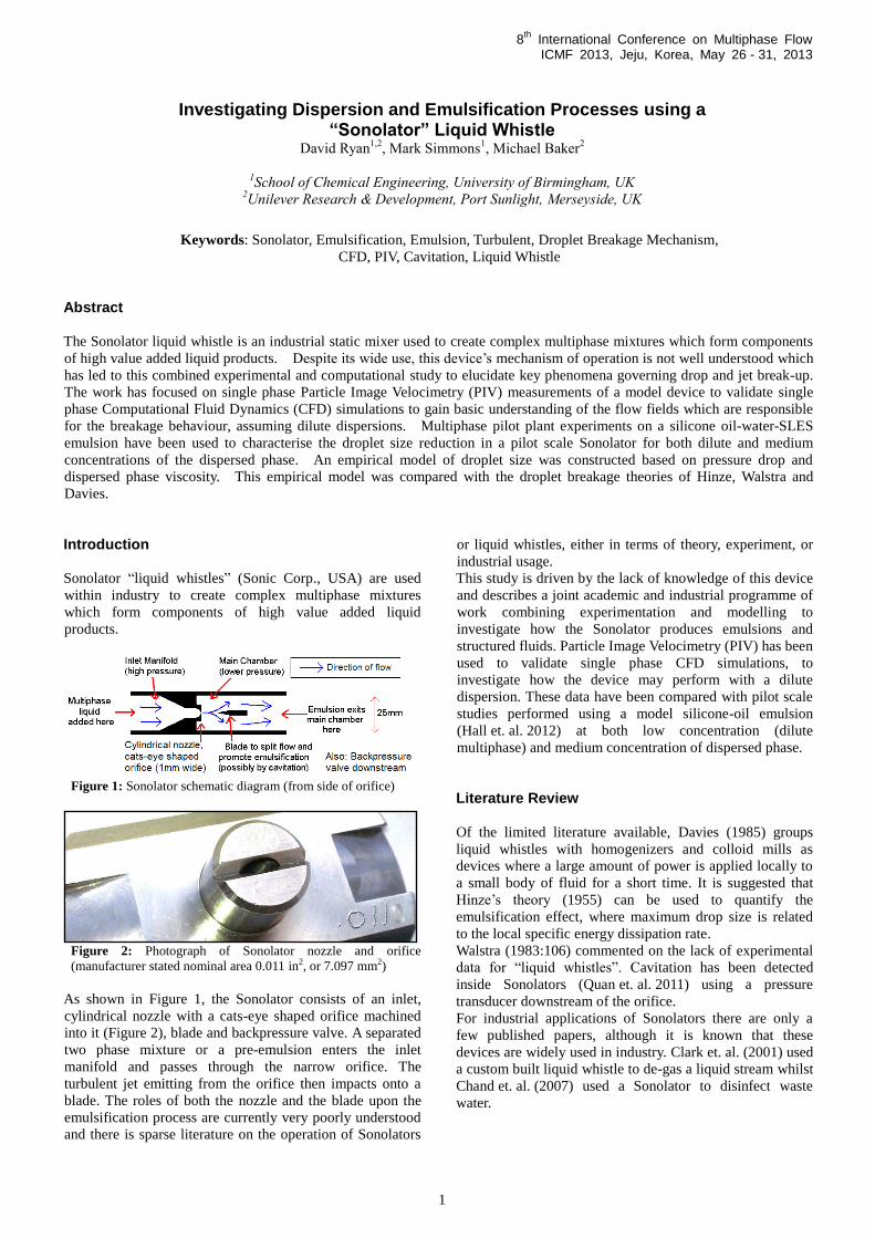
Figure 1: Sonolator schematic diagram (from side of orifice)

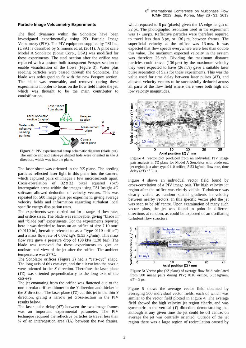
Figure 2: Photograph of Sonolator nozzle and orifice

(manufacturer stated nominal area 0.011 in2, or 7.097 mm2)

As shown in Figure 1, the Sonolator consists of an inlet,

cylindrical nozzle with a cats-eye shaped orifice machined

into it (Figure 2), blade and backpressure valve. A separated

two phase mixture or a pre-emulsion enters the inlet

manifold and passes through the narrow orifice. The

turbulent jet emitting from the orifice then impacts onto a

blade. The roles of both the nozzle and the blade upon the

emulsification process are currently very poorly understood

and there is sparse literature on the operation of Sonolators

or liquid whistles, either in terms of theory, experiment, or

industrial usage.

This study is driven by the lack of knowledge of this device

and describes a joint academic and industrial programme of

work combining experimentation and modelling to

investigate how the Sonolator produces emulsions and

structured fluids. Particle Image Velocimetry (PIV) has been

used to validate single phase CFD simulations, to

investigate how the device may perform with a dilute

dispersion. These data have been compared with pilot scale

studies performed using a model silicone-oil emulsion

(Hall et. al. 2012) at both low concentration (dilute

multiphase) and medium concentration of dispersed phase.

Literature Review

Of the limited literature available, Davies (1985) groups

liquid whistles with homogenizers and colloid mills as

devices where a large amount of power is applied locally to

a small body of fluid for a short time. It is suggested that

Hinze’s theory (1955) can be used to quantify the

emulsification effect, where maximum drop size is related

to the local specific energy dissipation rate.

Walstra (1983:106) commented on the lack of experimental

data for “liquid whistles”. Cavitation has been detected

inside Sonolators (Quan et. al. 2011) using a pressure

transducer downstream of the orifice.

For industrial applications of Sonolators there are only a

few published papers, although it is known that these

devices are widely used in industry. Clark et. al. (2001) used

a custom built liquid whistle to de-gas a liquid stream whilst

Chand et. al. (2007) used a Sonolator to disinfect waste

water.

8th


2

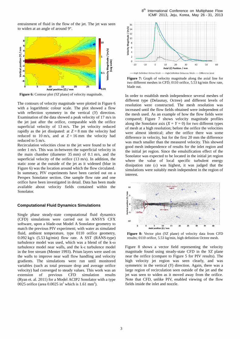
Particle Image Velocimetry Experiments

The fluid dynamics within the Sonolator have been

investigated experimentally using 2D Particle Image

Velocimetry (PIV). The PIV equipment supplied by TSI Inc.

(USA) is described by Simmons et. al. (2011). A pilot scale

Model A Sonolator (Sonic Corp., USA) was modified for

these experiments. The steel section after the orifice was

replaced with a custom-built transparent Perspex section to

enable visualisation of the flows (Figure 3). Water plus

seeding particles were passed through the Sonolator. The

blade was redesigned to fit with the new Perspex section.

The blade was removable, and removed during these

experiments in order to focus on the flow field inside the jet,

which was thought to be the main contributor to

emulsification.

Figure 3: PIV experimental setup schematic diagram (blade out).

The orifice slit and cats-eye shaped hole were oriented in the X

direction, which was into the plane.

The laser sheet was oriented in the YZ plane. The seeding

particles reflected laser light in this plane into the camera,

which captured pairs of images a few microseconds apart.

Cross-correlation of 32 x 32 pixel squared (px2)

interrogation areas within the images using TSI Insight 4G

software allowed deduction of velocity vectors. This was

repeated for 500 image pairs per experiment, giving average

velocity fields and information regarding turbulent local

specific energy dissipation rates.

The experiments were carried out for a range of flow rates

and orifice sizes. The blade was removable, giving “blade in”

and “blade out” experiments. For the experiments reported

here it was decided to focus on an orifice of size 7.10 mm2

(0.0110 in2, hereafter referred to as a “type 0110 orifice”)

and a mass flow rate of 0.092 kg/s (5.53 kg/min). This mass

flow rate gave a pressure drop of 138 kPa (1.38 bar). The

blade was removed for these experiments to give an

unobstructed view of the jet after the orifice. The ambient

temperature was 27°C.

The Sonolator orifices (Figure 2) had a “cats-eye” shape.

The long axis of this cats-eye, and the slit cut into the nozzle,

were oriented in the X direction. Therefore the laser plane

(YZ) was oriented perpendicularly to the long axis of the

cats-eye.

The jet emanating from the orifice was flattened due to the

non-circular orifice: thinner in the Y direction and thicker in

the X direction. The laser plane (YZ) cut this jet in the thin Y

direction, giving a narrow jet cross-section in the PIV

results below.

The laser pulse delay (dT) between the two image frames

was an important experimental parameter. The PIV

technique required the reflective particles to travel less than

¼ of an interrogation area (IA) between the two frames,

which equated to 8 px (pixels) given the IA edge length of

32 px. The photographic resolution used in the experiment

was 17 μm/px. Reflective particles were therefore required

to travel less than 8 px, or 136 μm, between frames. The

superficial velocity at the orifice was 13 m/s. It was

expected that flow speeds everywhere were less than double

this value. The maximum expected velocity in the system

was therefore 26 m/s. Dividing the maximum distance

particles could travel (136 μm) by the maximum velocity

they were expected to have (26 m/s) gave a suitable laser

pulse separation of 5 μs for these experiments. This was the

value used for time delay between laser pulses (dT), and

allowed velocity vectors to be successfully deduced across

all parts of the flow field where there were both high and

low velocity magnitudes.

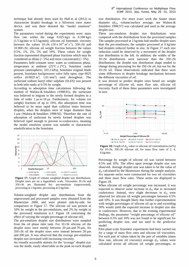
Figure 4: Vector plot produced from an individual PIV image

pair analysis in YZ plane for Model A Sonolator with blade out,

jet region just after type 0110 orifice, 5.53 kg/min flow rate, time

delay (dT) of 5 µs.

Figure 4 shows an individual vector field found by

cross-correlation of a PIV image pair. The high velocity jet

region after the orifice was clearly visible. Turbulence was

clearly visible as random spatial gradients in velocity

between nearby vectors. In this specific vector plot the jet

was seen to be off centre. Upon examination of many such

vector plots, the jet was found to point in different

directions at random, as could be expected of an oscillating

turbulent flow structure.

Figure 5: Vector plot (YZ plane) of average flow field calculated

from 500 image pairs during PIV; 0110 orifice, 5.53 kg/min,

dT = 5 µs.

Figure 5 shows the average vector field obtained by

averaging 500 individual vector fields, each of which was

similar to the vector field plotted in Figure 4. The average

field showed the high velocity jet region clearly, and was

symmetric in the vertical (Y) direction, demonstrating that

although at any given time the jet could be off centre, on

average the jet was centrally oriented. Outside of the jet

region there was a large region of recirculation caused by

8th


3

entrainment of fluid in the flow of the jet. The jet was seen

to widen at an angle of around 9°.

Figure 6: Contour plot (YZ plane) of velocity magnitude.

The contours of velocity magnitude were plotted in Figure 6

with a logarithmic colour scale. The plot showed a flow

with reflection symmetry in the vertical (Y) direction.

Examination of the data showed a peak velocity of 17 m/s in

the jet just after the orifice, comparable with the orifice

superficial velocity of 13 m/s. The jet velocity reduced

rapidly as the jet dissipated: at Z = 8 mm the velocity had

reduced to 10 m/s, and at Z = 16 mm the velocity had

reduced to 5 m/s.

Recirculation velocities close to the jet were found to be of

order 1 m/s. This was in-between the superficial velocity in

the main chamber (diameter 35 mm) of 0.1 m/s, and the

superficial velocity of the orifice (13 m/s). In addition, the

static zone at the outside of the jet as it widened (blue in

Figure 6) was the location around which the flow circulated.

In summary, PIV experiments have been carried out on a

Perspex Sonolator section. One sample flow rate and one

orifice have been investigated in detail. Data has been made

available about velocity fields contained within the

Sonolator.

Computational Fluid Dynamics Simulations

Single phase steady-state computational fluid dynamics

(CFD) simulations were carried out in ANSYS CFX

software, upon a blade-out Model A Sonolator geometry to

match the previous PIV experiment; with water as simulated

fluid, ambient temperature, type 0110 orifice geometry,

0.092 kg/s (5.53 kg/min) flow rate. A SST (RANS-type)

turbulence model was used, which was a blend of the k-ω

turbulence model near walls, and the k-ε turbulence model

in the free stream (Menter 1993). Prism layers were used on

the walls to improve near wall flow handling and velocity

gradients. The simulations were run until monitored

variables (such as total pressure drop and average orifice

velocity) had converged to steady values. This work was an

extension of previous CFD simulation results

(Ryan et. al. 2011) for a Model ACIP2 Sonolator with a type

0025 orifice (area 0.0025 in2 which is 1.61 mm

2).

Figure 7: Graph of velocity magnitude along the axial line for

two different meshes in CFD; 0110 orifice, 5.53 kg/min flow rate,

blade out.

In order to establish mesh independence several meshes of

different type (Delaunay, Octree) and different levels of

resolution were constructed. The mesh resolution was

increased until the flow fields obtained were independent of

the mesh used. As an example of how the flow fields were

compared; Figure 7 shows velocity magnitude profiles

along the Sonolator axis (X = Y = 0) for two different types

of mesh at a high resolution; before the orifice the velocities

were almost identical; after the orifice there was some

difference in velocity, but for the first 20 mm the difference

was much smaller than the measured velocity. This showed

good mesh independence of results for the inlet region and

the initial jet region. Since the emulsification effect of the

Sonolator was expected to be located in the initial jet region

where the value of local specific turbulent energy

dissipation rate (ε) was highest, it was judged that the

simulations were suitably mesh independent in the region of

interest.

Figure 8: Vector plot (YZ plane) of velocity data from CFD

results; 0110 orifice, 5.53 kg/min, high definition Octree mesh.

Figure 8 shows a vector field representing the velocity

magnitude found using steady-state CFD in the YZ plane

near the orifice (compare to Figure 5 for PIV results). The

high velocity jet region was seen clearly, and was

symmetric in the vertical (Y) direction. Again, there was a

large region of recirculation seen outside of the jet and the

jet was seen to widen as it moved away from the orifice.

Note that CFD, unlike PIV, enabled viewing of the flow

fields inside the inlet and nozzle.

8th


4

Figure 9: Contour plot (YZ plane) of velocity magnitude.

The contours of velocity magnitude for these CFD results

were plotted in Figure 9 with a logarithmic colour scale

(compare to Figure 6 for PIV results). The plot showed a

flow with nearly exact reflection symmetry in the vertical

(Y) direction. The peak velocity just after the orifice was

17 m/s, comparable with the superficial velocity at the

orifice of 13 m/s. Recirculation velocities were again of the

order 1 m/s, higher than the main chamber superficial

velocity of 0.1 m/s.

The turbulence model used in the CFD simulation gave

values for local specific turbulent energy dissipation rate,

(epsilon, ε). This quantity is measured as power per unit

mass, with units W/kg. Epsilon was thought to be a useful

quantity for predicting droplet size in emulsification (e.g.

Hinze 1955). Data concerning epsilon from single phase

CFD may be useful in understanding emulsification in

dilute multiphase systems, as discussed later in the pilot

plant results.

Figure 10: Graph of epsilon (ε) along the axial line. Epsilon is

shown on a logarithmic scale.

In Figure 10 epsilon was plotted against position (c.f.

Hakansson et. al. 2009:1179) along the Sonolator axis. This

variable was found to take values over many orders of

magnitude, from less than 1 W/kg before the orifice to over

1000 W/kg after the orifice. At the orifice there was a slight

peak in epsilon, but the main peak was achieved 10 mm

downstream from the orifice. This peak value was of order

5000 W/kg. Subsequently, epsilon declined at an

exponential rate over 30 mm.

Using sets of streamlines constructed in ANSYS CFD-Post

which followed the flow from the inlet through the orifice

and into the main chamber, graphs of epsilon vs time were

also considered. These graphs had similar shape to Figure

10. They showed that epsilon was near the peak value for a

time of order 100 µs to 1000 µs, the exact time depending

on the flow rate and on how close to the peak epsilon was

required to be. The duration that the fluid was subjected to

turbulent forces near the peak value of epsilon was thought

to be of importance for understanding emulsification.

In summary, CFD simulations have been carried out on a

Model A Sonolator geometry for the 0110 orifice type.

Mesh independence was checked, and flow fields were

obtained throughout the whole geometry, including in the

inlet and orifice. Turbulent dissipation rates were

investigated in order to check likely conditions for

emulsification of dilute multiphase fluids.

Validation of CFD using PIV

It was necessary to validate the CFD simulation results

against the PIV experimental results in order to have

confidence that the CFD results were accurate. Several

comparisons between the two sets of results were carried

out to complete this validation process. The comparisons

took the form of graphs of velocity vs position. The position

was varied over four different trajectories through the 3D

geometry, as shown in Figure 11.

Figure 11: Schematic diagram (YZ plane) for the Sonolator

showing the four trajectories used for validation: along the axis,

on a vertical line at Z = 5 mm, on similar lines at 10 mm and

20 mm.

CFD velocities were available throughout the whole system,

however PIV velocities were only available in the

transparent viewing chamber of the Sonolator (grey in

schematic diagram).

Figure 12: Graph of velocity magnitude along the axial line.

CFD and PIV results compared for a type 0110 orifice with mass

flow rate 5.53 kg/min, blade out.

Along the Sonolator axis (the line X = Y = 0 mm) both CFD

and PIV showed a peak in velocity of magnitude 17 m/s

about 1 mm after the orifice in the jet region (Figure 12);

the difference between PIV and CFD results was lowest

there. The difference between velocities was less than

1.4 m/s along the axis up to 20 mm. Moving downstream,

velocity reduced at approximately the same rate in the two

data sets; slightly faster in PIV. Overall agreement between

the two data sets was good up to 15 mm along the axial line.

8th


5

Figure 13: Graph of velocity magnitude vs vertical (Y) position

on the line segment at Z = 5 mm.

On the line in the Y direction at Z = 5 mm (and X = 0 mm)

cross-sections for the velocity profile were obtained for both

CFD and PIV results (Figure 13). In both sets of results the

jet was seen as a peak in velocity on the centreline

(Y = 0 mm). Since these results were 5 mm downstream

from the orifice, the peak velocity had declined from 17 m/s

to 13 m/s. Between PIV and CFD, the differences in

velocity within the jet were much smaller than the recorded

velocities, outside the jet in most places the differences were

smaller than the velocities, demonstrating that the CFD

simulation was of suitable accuracy.



Further downstream, on the line segment 10 mm after the

orifice (Figure 14), velocity within the jet peaked at around

9 m/s, with difference between experiment and simulation

less than 1.4 m/s. Across the rest of the cross-section, the

velocity difference was mostly lower than the measurements,

again showing reasonable agreement between PIV and

CFD.



On the line further downstream at Z = 20 mm (Figure 15),

the jet was seen as a velocity peak near the centreline

(Y = 0 mm) for both CFD and PIV. At this distance from the

orifice, differences started to appear between the two data

sources. The differences seen in velocity became

comparable with the sizes of the measurements, meaning

that CFD could not be validated this far away from the

orifice.

It was noted that the validation of CFD by PIV was

generally good near the orifice and generally poorer in the

regions further downstream. In these regions the CFD had a

tendency to converge to a flow field that was not fully

symmetric, thus losing the agreement between CFD and the

PIV average flow field. Although the PIV average flow field

was symmetric (Figure 5), representing the time-averaged

component of the actual transient velocity field, the

individual PIV snapshots (e.g. Figure 4) were not symmetric.

The jet motion seen between different PIV snapshots

highlighted a jet instability which tended to make the jet

direction fluctuate up and down. It is therefore thought that

the steady state CFD struggled to converge far downstream

of the orifice, where in the actual transient flow a large

amount of uncertainty in the jet position existed due to the

jet instability.

Pilot Plant Experiments with a Model Emulsion

Experiments have been performed to characterise droplet

breakage on a pilot plant Model ACIP2 Sonolator (Sonic

Corp., USA). This Sonolator had the same orifice shape as

the Model A Sonolator investigated previously using PIV

and CFD. Droplet breakage was thought to occur in a

similar manner in the two Sonolator devices, with the same

droplet breakage mechanisms.

Figure 16: Schematic diagram of pilot plant Sonolator process.

A silicone oil in water pre-emulsion stabilised by SLES

surfactant was prepared in the oil phase stirred tank (see the

method of Tesch et. al. 2003:570). The rate of stirring was

moderate so that oil droplets in the tank would not be too

small. It was verified later that tank sample droplets were in

all cases reduced greatly in size by the Sonolation process,

therefore the pre-emulsion droplets were judged to be

coarse enough to characterise the emulsification effect of

the Sonolator. At least 30 minutes of gentle stirring was

given for droplet sizes to stabilise before processing.

During processing the pre-emulsion was then diluted to a

specified oil concentration using water with matching SLES

concentration from the aqueous phase tank. It was then

processed in the Sonolator, and the resulting emulsion was

sampled close to the Sonolator outlet through the low point

drain (schematic diagrams Figure 16 for whole process and

Figure 1 for Sonolator). Droplet size distributions were

obtained before and after processing using a Mastersizer

2000 particle size analyser (Malvern Instruments, UK). This

8th


6

technique had already been used by Hall et. al. (2012) to

characterise droplet breakage in a Silverson rotor stator

device, and was there denoted the “model emulsion”

system.

The parameters varied during the experiments were: mass

flow rate within the range 0.025 kg/s to 0.108 kg/s

(1.5 kg/min to 6.5 kg/min); silicone oil kinematic viscosity

between the values 10 cSt (10 x 10-6

m2 s

-1), 350 cSt and

10 000 cSt; silicone oil weight fraction between the values

0.5%, 1%, 2%, 5% and 10%. These values for weight

fraction represented dispersed phase fractions which may be

considered as dilute (< 5%) and more concentrated (> 5%).

Parameters held constant were: water as continuous phase,

temperature at ambient (25°C ± 2°C), Sonolator outlet

pressure (atmospheric; 101.3 kPa), Sonolator original blade

present, Sonolator backpressure valve fully open, type 0025

orifice (0.0025 in2; 1.61 mm

2) used throughout. The

surfactant sodium lauryl ether sulphate (SLES) was present

in both inlet tanks at 0.5% by weight.

According to adsorption time calculations following the

method of Walstra & Smulders (1998:81), the surfactant

was believed to migrate to the newly formed droplets in a

time of order 1 μs to 10 μs. Furthermore, for volume (or

weight) fractions of up to 10%, this adsorption time was

believed to be more rapid than collision times between

droplets, when the droplets were of larger diameter than

1 μm (Walstra & Smulders 1998:92). Therefore the rate of

adsorption of surfactant by newly formed droplets was

believed rapid enough to prevent re-coalescence, meaning

the model emulsion system was suitable to characterise

emulsification in the Sonolator.

Figure 17: Graph of volume weighted droplet size distributions.

Droplet sizes are on a logarithmic scale. Viscosities 10 cSt and

350 cSt are illustrated for: pre-emulsion (unprocessed),

processing at 2 kg/min, processing at 6 kg/min.

Volume-weighted droplet size distributions from the

unprocessed and processed samples were obtained from the

Mastersizer 2000, and were plotted side-by-side for

comparison in Figure 17. The silicone oil was present at

10% by weight in the pre-emulsions, and 2% by weight in

the processed emulsions (c.f. Figure 18 concerning the

effect of varying the weight percentage of silicone oil).

The pre-emulsion droplet size distributions were sampled

from the oil phase inlet tank. For 10 cSt silicone oil the

droplet sizes were mostly between 20 μm and 70 μm; for

350 cSt oil the droplet sizes were instead between 20 μm

and 200 μm. It was observed that the average pre-emulsion

droplet size increased with increasing viscosity.

An visually accessible statistic for the “average” droplet size

was the mode, easily observable as the peak on each droplet

size distribution. For more exact work the Sauter mean

diameter (d32, volume/surface average; see Walstra &

Smulders 1998:57) was calculated and used as the average

droplet size.

These pre-emulsion droplet size distributions were

compared with the distributions from the processed samples.

The samples processed at 2 kg/min had smaller droplet sizes

than the pre-emulsions; the samples processed at 6 kg/min

had droplets reduced further in size. In Figure 17 each size

reduction could be observed by a movement of the droplet

size distribution to the left. In addition: the widths of the

10 cSt distributions were narrower than the 350 cSt

distributions; the droplet size distribution shape tended to

change during processing for the 350 cSt oil, but not for the

10 cSt oil. These observations indicated that there were

some differences in droplet breakage mechanism between

the different viscosities of oil.

It was desired to predict droplet sizes based on: weight

percentage of silicone oil, mass flow rate, silicone oil

viscosity. Each of these three parameters were investigated

in turn.

Figure 18: Graph of d32 value vs silicone oil concentration (wt%)

for 10 cSt, 350 cSt silicone oil, for mass flow rates of 2, 4,

6 kg/min.

Percentage by weight of silicone oil was varied between

0.5% and 10%. The effect upon average droplet size was

observed. Average droplet size was taken to be the value of

d32 calculated by the Mastersizer during the sample analysis.

Six separate series were constructed for two oil viscosities

and three mass flow rates. These series are displayed in

Figure 18.

When silicone oil weight percentage was increased, it was

expected to observe some increase in d32 due to increased

coalescence. Instead, very slight decreases in d32 were

observed for silicone oil weight percentages between 0.5%

and 10%. It was thought likely that further experimentation

with weight percentages of silicone oil up to and exceeding

50% would yield the expected increase in droplet size due

to coalescence. However, due to the existing experimental

findings, the parameter “weight percentage of silicone oil”

between 0.5% and 10% was not found to be significant for

predicting droplet size, and not used in the predictive

model.

Pilot plant scale Sonolator experiments had been carried out

for a range of mass flow rates and silicone oil viscosities.

For each pair of values taken by the pair of variables (mass

flow rate, silicone oil viscosity) average d32 values were

calculated across all silicone oil weight percentages, to

8th


7

make effective use of all data, since the latter parameter

(silicone oil weight percentage) had been found

insignificant. Mass flow rate had been varied between

1.5 kg/min and 6.5 kg/min; viscosity was varied between

10 cSt, 350 cSt and 10 000 cSt; the average d32 values are

presented in Figure 19:

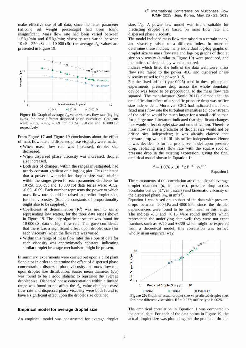
Figure 19: Graph of average d32 value vs mass flow rate (log-log

axes), for three different dispersed phase viscosities. Gradients

were: -0.52, -0.65, -0.69 for 10 cSt, 350 cSt and 10 000 cSt

respectively.

From Figure 17 and Figure 19 conclusions about the effect

of mass flow rate and dispersed phase viscosity were made:

When mass flow rate was increased, droplet size

decreased.

When dispersed phase viscosity was increased, droplet

size increased.

Both sets of changes, within the ranges investigated, had

nearly constant gradient on a log-log plot. This indicated

that a power law model for droplet size was suitable

within the ranges given for each parameter. Gradients for

10 cSt, 350 cSt and 10 000 cSt data series were: -0.52,

-0.65, -0.69. Each number represents the power to which

mass flow rate should be raised to predict droplet size,

for that viscosity. (Suitable constants of proportionality

ought also to be supplied.)

Coefficient of determination (R2) was near to unity,

representing low scatter, for the three data series shown

in Figure 19. The only significant scatter was found for

10 000 cSt data at high flow rate. This gave confidence

that there was a significant effect upon droplet size (for

each viscosity) when the flow rate was varied.

Within this range of mass flow rates the slope of data for

each viscosity was approximately constant, indicating

similar droplet breakage mechanisms might be present.

In summary, experiments were carried out upon a pilot plant

Sonolator in order to determine the effect of dispersed phase

concentration, dispersed phase viscosity and mass flow rate

upon droplet size distribution. Sauter mean diameter (d32)

was found to be a good statistic to represent the average

droplet size. Dispersed phase concentration within a limited

range was found to not affect the d32 value obtained; mass

flow rate and dispersed phase viscosity were both found to

have a significant effect upon the droplet size obtained.

Empirical model for average droplet size

An empirical model was constructed for average droplet

size, d32. A power law model was found suitable for

predicting droplet size based on mass flow rate and

dispersed phase viscosity.

The model included mass flow rate raised to a certain index,

and viscosity raised to a different index. In order to

determine these indices, many individual log-log graphs of

droplet size vs mass flow rate and log-log graphs of droplet

size vs viscosity (similar to Figure 19) were produced, and

the indices of dependency were compared.

Indices which fitted the bulk of the data well were: mass

flow rate raised to the power -0.6, and dispersed phase

viscosity raised to the power 0.15.

For the fixed orifice (type 0025) used in these pilot plant

experiments, pressure drop across the whole Sonolator

device was found to be proportional to the mass flow rate

squared. The manufacturer (Sonic 2011) claimed that the

emulsification effect of a specific pressure drop was orifice

size independent. Moreover, CFD had indicated that for a

fixed mass flow rate the turbulent intensities (ε) downstream

of the orifice would be much larger for a small orifice than

for a large one. Literature indicated that significant changes

in ε would affect droplet size and emulsification. Therefore

mass flow rate as a predictor of droplet size would not be

orifice size independent; it was already claimed that

pressure drop would fulfil this orifice independence. Hence

it was decided to form a predictive model upon pressure

drop, replacing mass flow rate with the square root of

pressure drop in the existing expression, giving the final

empirical model shown in Equation 1:

Equation 1

The components of this correlation are dimensional: average

droplet diameter (d, in metres), pressure drop across

Sonolator orifice (ΔP, in pascals) and kinematic viscosity of

the dispersed phase (νD, in m2 s

-1).

Equation 1 was based on a subset of the data with pressure

drops between 200 kPa and 4000 kPa since the droplet

dependencies were found to be most linear in this range.

The indices -0.3 and +0.15 were round numbers which

represented the underlying data well; they were not exact

fractions such as -6/20 and +3/20 which might be expected

from a theoretical model; this correlation was formed

wholly in an empirical way.

Figure 20: Graph of actual droplet size vs predicted droplet size,

for three different viscosities. R2 = 0.977; orifice type is 0025.

The empirical correlation in Equation 1 was compared to

the actual data. For each of the data points in Figure 19, the

actual droplet size was plotted against the predicted droplet

8th


8

size to give Figure 20. This included the diagonal line

(actual = predicted) which represented 100% accuracy for

this correlation. The data was very close to the diagonal,

with low scatter and coefficient of determination (R2) above

0.97, showing that this correlation fitted the data well.

Identification of droplet breakage regime

Different droplet breakage regimes are described in the

literature, based on whether the flow is laminar or turbulent,

and how the size of the droplets compares to the minimum

turbulent eddy length scale (the Kolmogorov length scale).

A comparison was made between the flow conditions in the

pilot plant experiments described above with the regimes

described in literature.

Equation 2

Equation 3

Table 1: Reynolds numbers and Kolmogorov length scales at

orifice and main chamber, for low and high flow rates.

Equations for Reynolds number (Re) and Kolmogorov

length scale (le) (Kolmogorov 1949) are given in Equation 2

and Equation 3 respectively. Calculations are given in Table

1 for the maximum and minimum of Reynolds numbers and

Kolmogorov length scales, according to the ranges of mass

flow rates and oil viscosities investigated during the pilot

plant experiments.

At the orifice the Reynolds number (Equation 2) was

between 15 000 and 67 000. Since a Reynolds number

above 10 000 indicated fully turbulent flow, the flow was

deduced to be fully turbulent at the orifice at all flow rates

during the pilot plant experiments.

Far downstream from the orifice the superficial velocity was

low (0.02 m/s to 0.12 m/s), with Reynolds numbers between

900 and 4000. However, as seen during PIV and CFD

studies (Figure 6 and Figure 9 respectively) typically the

local velocity in the jet dissipation region was 10 times the

main chamber superficial velocity. The true Reynolds

number in the dissipation region was therefore

9000 to 40 000. Hence the flow stayed fully turbulent

throughout the region of emulsification. This meant that

laminar droplet disruption mechanisms could be discounted.

Walstra & Smulders (1998:59) give two main droplet

disruption regimes in turbulent flow: turbulent viscous (TV)

and turbulent inertial (TI). For regime TV, droplets are

typically smaller than all turbulent eddies. The smallest

eddies have diameters of the order of the Kolmogorov

length scale (Equation 3). Droplets break within these

eddies because of the viscous shear stresses. Conversely, for

regime TI, droplets are typically larger than the

Kolmogorov length scale and are broken by random

pressure fluctuations from the surrounding turbulent eddies.

Both of these different regimes give a different correlation

between droplet size and flow parameters.

To calculate the Kolmogorov length scale, epsilon (ε) had to

be estimated in the jet dissipation region. Based on the

largest values of epsilon obtained from CFD simulations

(Figure 10) a model was constructed for peak epsilon based

on flow rate and orifice size. Subsequently, epsilon

calculations were added (Table 1) to the pilot plant data, and

Kolmogorov length scales were found to be between

2.5 µm and 0.83 µm as the flow rate increased from

1.5 kg/min to 6.5 kg/min.

The largest Kolmogorov length scale obtained was 2.5 µm

at low flow rate, and the smallest average droplet size (d32)

was over 3 µm at high flow rate (Figure 19). It was

therefore concluded that for these pilot plant experiments on

the Sonolator, with water as the continuous phase, droplets

were always larger than the Kolmogorov length scale, the

break-up regime was always turbulent, and that therefore

the break-up regime was turbulent inertial (TI) throughout

these pilot plant trials.

Comparison of empirical model with turbulent inertial (TI) correlations and experimental data described in the literature

Literature exists describing theories concerning how the

droplet size changes with epsilon and dispersed phase

viscosity in the turbulent inertial (TI) droplet break-up

regime. Experimental results for the same regime also exist.

Both are compared to the empirical model for average

droplet size obtained above. All the theoretical and

experimental results are in the form of power laws. These

are convenient because the effect of each term is

independent, i.e. in the power law model epsilon has an

independent effect on droplet size from the effect of

viscosity. Power laws are also convenient since, when

comparing them, one need only compare the relative indices

of matching variables.

Table 2: Theoretical correlations for droplet size.

Author Droplet size (d)

proportional to:

Hinze (1955) ε-0.4

ρC-0.6

σ0.6

Walstra & Smulders

(1998:71)

ε-0.25

ρC-0.75

µD0.75

Davies (1987) ε-0.4

ρC-0.6

σ0.6

(1+ βµD u′/ σ)0.6

Note: u′ can be approximated

by (ε d)1/3. Also note that the

scaling constant β was estimated

at 0.7 for Newtonian fluids.

Hinze (1955) considered droplet break-up at equilibrium in

regime TI, with non-coalescing conditions (dilute dispersed

phase), isotropic homogenous turbulence and low viscosity

of dispersed phase. The proportionality Hinze obtained for

dmax is given in Table 2. dmax is the maximum droplet size

8th


9

which is expected to be stable in regime TI. If the shape of

the droplet size distribution does not change (on a

logarithmic size axis) as the average droplet size reduces,

d32 is also proportional to the same expression. (The

constant of proportionality would be reduced when going

from dmax to d32.)

Walstra & Smulders (1998) considered regime TI for

droplets where high viscosity hindered breakage time. Their

proportionality was dependent upon dispersed phase

viscosity (µD) instead of interfacial tension (σ), since the

limiting factor in droplet break-up had changed.

Davies (1987) previously had modified Hinze’s expression

by adding to the cohesive force due to interfacial tension an

extra cohesive term due to viscosity. In fact, with the

assumption given in Table 2 concerning the magnitude of u′,

for low viscosity Davies’ expression reduces to that of

Hinze, and for high viscosity it reduces to that of Walstra.

To conclude the literature survey on theoretical droplet

breakage mechanisms in regime TI: there are a range of

droplet size models for low and high dispersed phase

viscosity. Those given above agree with one another in

terms of power law dependency upon epsilon (ε),

continuous phase density (ρC), interfacial tension (σ) and

dispersed phase viscosity (µD).

Table 3: Experimental results for droplet size.

Author Droplet size (d)

proportional to:

Ryan (empirical droplet

size model given above) on

Sonolator

µD0.15

ε-0.2

or

µD0.15

ΔP-0.3

Walstra & Smulders (1998:72)

on UltraTurrax, high pressure

homogenizer (HPH)

µD0.33

Karbstein (1994) on HPH µD0.4

Pandolfe (1981) on HPH µD0.7

Experimental correlations also appear in the literature,

which are given in Table 3 along with the empirical model.

Comparing dispersed phase viscosity (µD) between Table 2

and Table 3: the range of viscosity indices in the

experimental results is [0.33, 0.7]; the empirical model

developed above in this paper has a slightly lower viscosity

index of 0.15; the theoretical results give bounds on

viscosity index of 0 (Hinze) and 0.75 (Walstra & Smulders),

and predict a smooth transition regime in-between (Davies).

All the experimental results fit into the theoretical bounds of

[0, 0.75]. The range of experimental results for a high

pressure homogenizer (HPH) is [0.33, 0.7] and these

differences are not explained in the literature when

mentioned by Walstra & Smulders (1998:72).

HPH and Sonolator are superficially similar systems since

both involve forcing a fluid through a small gap and both

have a jet-like region with high fluid velocity and epsilon

(for HPH results see Hakansson et. al. 2009). Due to this

similarity, an explanation is needed for the difference

between Sonolator index (0.15) and HPH indices [0.33,

0.7].

The Sonolator index of viscosity (0.15) was constructed

from multiple graphs of droplet size vs dispersed phase

viscosity (on log-log axes) across the whole range of

viscosities from 10 cSt to 10 000 cSt, and utilising some

additional data at 3.8 cSt. It was not noted that for low

viscosity the slope was approximately 0 (as per Hinze 1955),

with a relatively quick transition at higher viscosity to slope

of 0.75 (as per Walstra & Smulders 1998); the absence of

such an observation contradicts Davies’ model (1987) which

predicts these two distinct regions. Instead, the overall slope

of 0.15 appeared to be nearly constant across the whole

range of viscosities, when flow rate was held constant at

various levels. Walstra (1993:340) also expressed

reservations about Davies’ derivation, and provided

experimental evidence on various devices showing a power

law (constant slope) dependency of droplet size upon

viscosity.

In summary concerning droplet size dependency upon

dispersed phase viscosity: the experimental results were

within the bounds provided by theoretical considerations.

Differences exist between the experimental results which

await further explanation. The way the different theoretical

models fit together is likely to be more gradual than

indicated by Davies (1987).

Equation 4

Epsilon should scale according to Equation 4 from

dimensional considerations. Length scale (L) and velocity

(u) are characteristic for the system. C1 is a numerical

constant (as are Ci in subsequent equations below). For any

Sonolator with fixed orifice and main chamber geometry, i.e.

fixed L, epsilon should therefore be proportional to flow

rate cubed. Examination of CFD simulation results found

that this rule was followed reasonably closely. Since

pressure drop was found to be proportional to flow rate

squared, epsilon was therefore proportional to pressure drop

to the index 3/2. The empirical model for experimental data

for the Sonolator stated that droplet size was proportional to

pressure drop to the power -0.3, which is thus equivalent to

epsilon to the power -0.2, as given in Table 3.

This sits at odds with the theoretical models in Table 2. For

low viscosity, Hinze (1955) gives index of epsilon of -0.4;

for high viscosity, Walstra & Smulders (1998) gave index of

-0.25, and for in-between cases Davies (1987) gave a

smooth transition between these two extremes with local

indices in the range [-0.4, -0.25].

Therefore the experimental data, as summarized by the

empirical model given, does not support any of the

theoretical models unless they are suitably modified.

It is in fact thought that a suitable modification can be made.

The assumption so far has been that interfacial tension was

constant during breakage, and so the interfacial tension term

(σ) in Hinze’s correlation was constant. However, the results

suggest that this assumption may have been erroneous.

One argument was in terms of an interfacial age concept: for

high epsilon, new interface was created at a faster rate than

at low epsilon. Diffusion of SLES surfactant (present in

excess) to the newly formed interfaces happened at

approximately a constant rate. Therefore, at high epsilon

newly created droplets had lower interfacial concentrations

of surfactant, hence higher interfacial tension; at low

epsilon newly created droplets had higher concentrations of

surfactant, hence lower interfacial tension. This introduced a

dependency of interfacial tension upon epsilon, whereas

previously interfacial tension was thought independent of

8th


10

epsilon. As shown below, this can suitably modify the

overall epsilon dependency to fit experimental results.

Equation 5

Returning to the overall problem of predicting droplet size;

it was clear that droplet size would depend both on surface

tension (Hinze) as well as viscosity (Walstra). However, a

different way was sought to combine the two models than

that of Davies. Since the viscosity dependence from

experiment was a power law, it was thought appropriate to

combine the Hinze and Walstra correlations according to a

joint power law with unknown exponents A and B, as per

Equation 5. A and B represent the relative effect of each

equation in predicting droplet size and are, at a first

approximation, constants.

C2 is a dimensionless constant; solving for A and B: for d to

be in metres, A + B = 1. Furthermore: 0.75 B = 0.15 to

achieve the correct index of viscosity. Therefore: A = 0.8,

B = 0.2, and the resulting equation was simplified to give

Equation 6:

Equation 6

Interfacial tension (σ) was now thought to be a function of

epsilon. Assuming that within a suitable range the

dependence of σ upon ε could expressed by another power

law:

Equation 7

In Equation 7 the constant C3 is dimensional; also the range

of applicability must be limited, since σ is limited above by

the interfacial tension of a clean interface, and limited below

by the interfacial tension of a surfactant saturated interface.

Substituting Equation 7 into Equation 6:

Equation 8

From the empirical model, the index of epsilon should be

-0.2. Therefore, from Equation 8, -0.2 = -0.37 + 0.48 N.

Solving: N = 0.354. This yields two final correlations:

Equation 9

Equation 10

So, based upon the assumption that power law dependencies

were reasonable throughout, Equation 9 was formed; a

semi-theoretical correlation combining Hinze’s and

Walstra’s theoretical correlations for droplet size, and

assuming that the experimental data should determine the

relative effect of each of the source correlations. Equation

10 is the required dependency of interfacial tension upon

epsilon. Note that this agrees with the interfacial age

concept previously discussed: high epsilon gives higher

interfacial tension, low epsilon gives lower interfacial

tension.

In order to check the range of epsilon values Equation 10

could be valid for: in Table 1, ε was found to vary from

25 700 W/kg to 2 090 000 W/kg, a factor of approximately

82. According to Equation 10, σ should consequently vary

by a factor of 4.7.

El-Hamouz (2007:802) gave σ for a water / silicone oil

interface as 42.5 mN/m, and for a water / 0.7 wt% SLES /

silicone oil interface as 13 mN/m, at 25°C; this σ varies by a

factor of 3.3. Since this experimental factor for σ is slightly

smaller than the 4.7 derived earlier, it is likely that the

power law approximation (Equation 10) is a good

approximation across most of the range of epsilon values

investigated above, but should not be extended to any

higher or lower values of epsilon due to σ being bounded by

the values for clean and saturated interfaces respectively.

In conclusion regarding the effect of epsilon upon droplet

size for droplet breakage in turbulent inertial flow:

theoretical models gave epsilon index in the range [-0.4,

-0.25]. The empirical model gave an epsilon index of -0.2.

These values appeared to be incompatible. Surfactant was

present in excess during droplet breakage. It was thought

likely that this led to a dependence of interfacial tension

upon epsilon. Using this modification, it was possible to

develop further correlations which harmonised theoretical

and empirical results.

Conclusions

The emulsification effect of a Sonolator liquid whistle was

investigated, due to there being sparse literature on the

subject. Two dimensional Particle Image Velocimetry (PIV)

experimentation was undertaken to measure the flow fields

inside the Sonolator. Computational Fluid Dynamics (CFD)

simulations were also carried out to find velocity, pressure

and epsilon fields inside the Sonolator in three dimensions.

The CFD was successfully validated by the PIV results,

allowing CFD to be used increasingly as a tool for

investigating the Sonolator.

Pilot plant experiments using a “model emulsion” (silicone

oil dilute dispersed phase, water continuous phase, SLES

surfactant) were carried out to characterise the change in

droplet size due to processing in the Sonolator under

different flow conditions. An empirical model was

constructed to predict droplet size from pressure drop and

dispersed phase viscosity. Dispersed phase weight fraction

between 0.5 wt% and 10 wt% was found to be insignificant

for predicting droplet size.

The droplet breakage regime was investigated and found to

be turbulent inertial (TI). The theoretical correlations of

Hinze, Walstra and Davies were provided from the literature

to compare to the empirical model. Although the basic

theoretical models did not agree with the empirical model, a

modification assuming interfacial tension dependence upon

epsilon yielded a plausible explanation of how theory and

experiment fitted together.

Acknowledgements

Neil Adams, Kim Jones (Unilever R&D Port Sunlight)

8th


11

for assistance with pilot plant experiments.

Adam Kowalski (Unilever R&D Port Sunlight) for

advice interpreting the pilot plant experimental results

with respect to surfactant effect, and for access to

supplementary pilot plant data.

Federico Alberini (School of Chemical Engineering,

University of Birmingham) for training on the PIV

equipment and software.

Andrea Gabriele (School of Chemical Engineering,

University of Birmingham) for training on ANSYS CFX.

Nomenclature

[M,N] numerical range. M and N are real numbers;

range is from lower bound M to upper bound N.

cSt centistokes, unit of kinematic viscosity;

equivalent to 10-6

m2 s

-1

Roman letters

A, B, N numerical constants

Ci numerical constants in correlations

d droplet size (m)

d32 Sauter mean diameter (m)

dmax Maximum stable droplet size in

turbulent flow (m)

dT delta-T; time delay between laser pulses in PIV (s)

L Characteristic length scale (m)

le Kolmogorov eddy length scale (m)

ΔP Pressure drop across Sonolator orifice (Pa)

px pixel, unit of length in a digital image

R2 Coefficient of determination, close to unity when

scatter is close to zero.

Re Reynolds Number

u velocity / characteristic velocity (m/s)

u′ time dependent component of velocity (m/s)

X, Y, Z position coordinates (m)

Greek letters

β beta, constant relating effect of viscosity to

interfacial tension

ε epsilon, local specific turbulent energy

dissipation rate (m2 s

-3 or W/kg)

νC kinematic viscosity of continuous phase (m2 s

-1)

νD nu, kinematic viscosity of dispersed phase (m2 s

-1)

µD mu, dynamic viscosity of dispersed phase (Pa s)

ρC rho, density of continuous phase(kg m-3

)

σ sigma, interfacial tension (N m-1

)

Subscripts

C continuous phase (water)

D discrete phase (oil)

e eddy

max maximum (droplet size)

References

Chand R., Bremner D. H., Namkung K. C., Collier P. K.,

Gogate P. R. Water disinfection using the novel approach of

ozone and a liquid whistle reactor. Biochemical Engineering

Journal 35 357-364 (2007)

Clark A., Dewhurst R. J., Payne P. A. Degassing a Liquid

Stream using an Ultrasonic Whistle. IEEE Ultrasonics

Symposium 579 (2001)

Davies J. T. Drop Sizes of Emulsions Related to Turbulent

Energy Dissipation Rates. Chem. Eng. Sci. 40 5 pp839-842

(1985)

Davies J. T. A Physical Interpretation of Drop Sizes in

Homogenizers and Agitated Tanks, Including the Dispersion

of Viscous Oils. Chem Eng Sci 42 7 pp1671-1676 (1987)

El-Hamouz A. Effect of Surfactant Concentration and

Operating Temperature on the Drop Size Distribution of

Silicon Oil Water Dispersion. J. Disp. Sci. Tech., 28

pp797-804 (2007)

Hakansson A., Tragardh C., Bergenstahl B. Studying the

effects of adsorption, recoalescence and fragmentation in a

high pressure homogenizer using a dynamic simulation

model. Food Hydrocolloids 23 pp1177-1183 (2009)

Hall S., Pacek A. W., Kowalski A. J., Cooke M., Rothman D.

The Effect of Scale on Liquid-liquid Dispersion in In-line

Silverson Rotor-Stator Mixers. 14th

European Conference

on Mixing, Warzawa. (2012)

Hinze J. O. Fundamentals of the Hydrodynamic Mechanism

of Splitting in Dispersion Processes. A.I.Ch.E. Journal 1 3,

pp289-295 (1955)

Karbstein H., Ph.D. Thesis, University of Karlsruhe (1994)

Kolmogorov A. N. The breakup of droplets in a turbulent

stream. Dokl. Akad. Nauk 66 pp825-828 (1949)

Menter F. R. Zonal Two Equation Kappa-Omega

Turbulence Models for Aerodynamic Flows. AIAA 24th

Fluid Dynamics Conference, Orlando, Florida (1993)

Pandolfe W.D. Effect of Dispersed and Continuous Phase

Viscosity on Droplet Size of Emulsions Generated by

Homogenization. J. Disp. Sci. Technol. 2 459 (1981)

Quan K-M., Avvaru B., Pandit A. B. Measurement and

Interpretation of Cavitation Noise in a Hybrid

Hydrodynamic Cavitating Device. A.I.Ch.E. Journal 57 4,

pp861-871 (2011)

Ryan D., Simmons M. J. H., Baker M. Modelling

Multiphase Jet Flows for High Velocity Emulsification.

Proceedings of ASME-JSME-KSME Joint Fluids

Engineering Conference 2011, Hamamatsu, Japan.

AJK2011-03023. (2011)

Simmons M. J. H., Alberini F., Tsoligkas A. N., Gargiuli J.,

Parker D. J., Fryer P. J., Robinson S. Development of a

hydrodynamic model for the UV-C inactivation of milk in a

novel ‘SurePure turbulatorTM

’ swirl-tube reactor. Innov.

Food Sci. Emerg. Tech. 14 pp122-134 (2012)

Sonic Corporation. Sonolator Homogenizing Systems

Operating and Instruction Manual (downloaded 1st July

8th


12

2011 from www.sonicmixing.com/ Manuals/

Sonolator_System_Manual.pdf) (2011)

Tesch S., Freudig B., Schubert H. Production of Emulsions

in High Pressure Homogenizers Part I: Disruption and

Stabilization of Droplets. Chem. Eng. Technol. 26 5

pp569-573 (2003)

Walstra P. Formation of Emulsions (Chapter 2 of

Encyclopedia of Emulsion Technology, ed. Becher P.)

pp57-127 (1983)

Walstra P. Principles of Emulsion Formation. Chem. Eng.

Sci. 48 2 pp333-349 (1993)

Walstra P., Smulders P. E. A. Emulsion Formation (Chapter

2 of Modern Aspects of Emulsion Science, ed. Binks B. P.)

pp56-99 (1998)

icmf2013-417 (conference paper dr) investigating dispersion and emulsification processes using a...

Documents