idac-4 - ockenfels syntech gmbhidac-4 intelligent data acquisition controller with programmable...
TRANSCRIPT
IDAC-4
Intelligent Data Acquisition Controller with programmable output control
AUTOSPIKE
Software for Signal Recording and Programmable Output Control
User's GUIDE
Rev. April 2004

© SYNTECH 2004
Hilversum, The Netherlands
Reproduction of text and/or drawings is permittedfor personal use. The use of reproductions in publicationsis only allowed if correct reference is made to SYNTECH
CONTENTS page INTRODUCTION 1 General INSTALLATION 2 Software Device Interface Program Hardware 3 SIGNAL CONNECTIONS 4 Input signals Output signals 5 OPERATION 6 Recording Record Control Bar 7 Record properties box Times Recording Trigger 8 File Spikes Digital 9 Mode FILTER SETTINGS and OFFSET CONTROL Input Filters WAVE FORM RECORDING 10 SPIKE DISCRIMINATION and SELECTION 13 SPIKE AMPLITUDE HISTOGRAM 14 SPIKE COUNTER 15 SPIKE FREQUENCY 16 AMPLITUDE and TIME MEASUREMENT 17 GRAPHICAL and NUMERICAL DATA TRANSFER 18 IDAC OUTPUT CONTROL General 19 Programming 20 Digital outputs Analog outputs 22 Trigger Synchronization 23
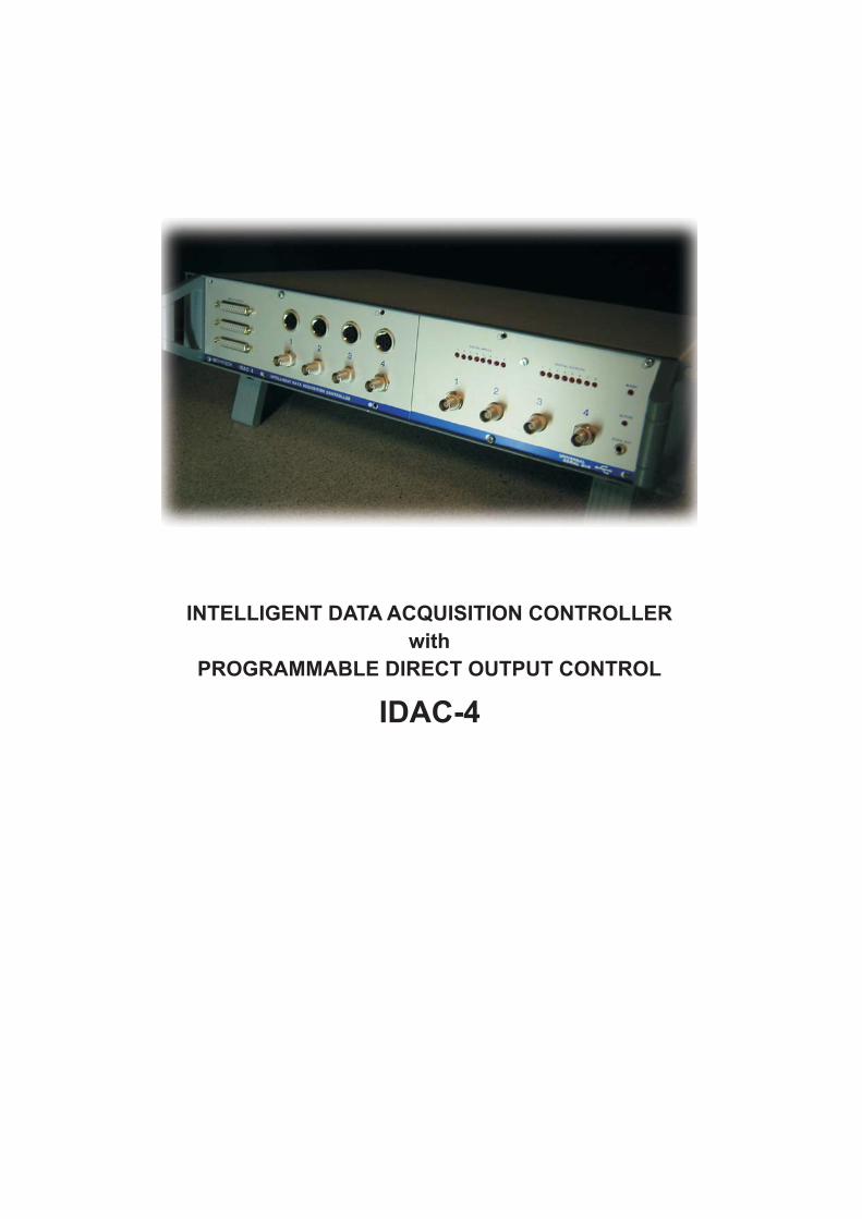
INTELLIGENT DATA ACQUISITION CONTROLLER
with
PROGRAMMABLE DIRECT OUTPUT CONTROL
IDAC-4

1
INTRODUCTION The instructions presented here are aimed to serve as a guide to the installation
and operation of the Syntech IDAC-4 and the application program Autospike. The IDAC-4 is a multi channel programmable data-acquisition
amplifier/controller for the USB (Universal Serial Bus) and was especially developed for physiological signal recording, storage, and analysis.
As with all novel instruments the user must invest some time and patience to gain sufficiently experience to operate the system smoothly.
There is no risk for any electronic damage to the system or any device connected to it, nor to the integrity of the program code if the system is setup without having consulted the instructions; Nevertheless, it is highly recommended to read and use the instructions during installation and first operation.
The present manual is far from complete; it is nothing more than a brief introduction to the many features and options of the system.
The best way of learning how to use the program is by exploration: just try out all possible settings, properties, and check the effect.
GENERAL The Syntech IDAC-4 is designed for multi channel synchronous data acquisition
for general electrophysiological research. The A/D and control circuits for the IDAC-4 are contained in a 19" box, which is connected to the PC via a single USB cable.
Up to 8 outputs for direct control of actuators (solenoids, valves etc) and 2
analog voltages can be programmed using the 'output control' module, which is part of Autospike. The output program can be synchronized with the signal acquisition.
The software runs on Windows98 and later Windows versions. During operation all signals are continuously displayed in oscilloscope style on
the PC screen at an adjustable time base. This facilitates fast and easy adjustment of signal levels, amplification factors, filter settings, and sampling rates, as the effect of changing a parameter is immediately visible.
The built-in power supply enables direct connection of input head stages and
transducers without additional wiring and power converters. Problems induced by ground loops are avoided as the power supply and all inputs and outputs are galvanically isolated.
2.
3.
4.
5.
6.
7.
8.
9.
10.
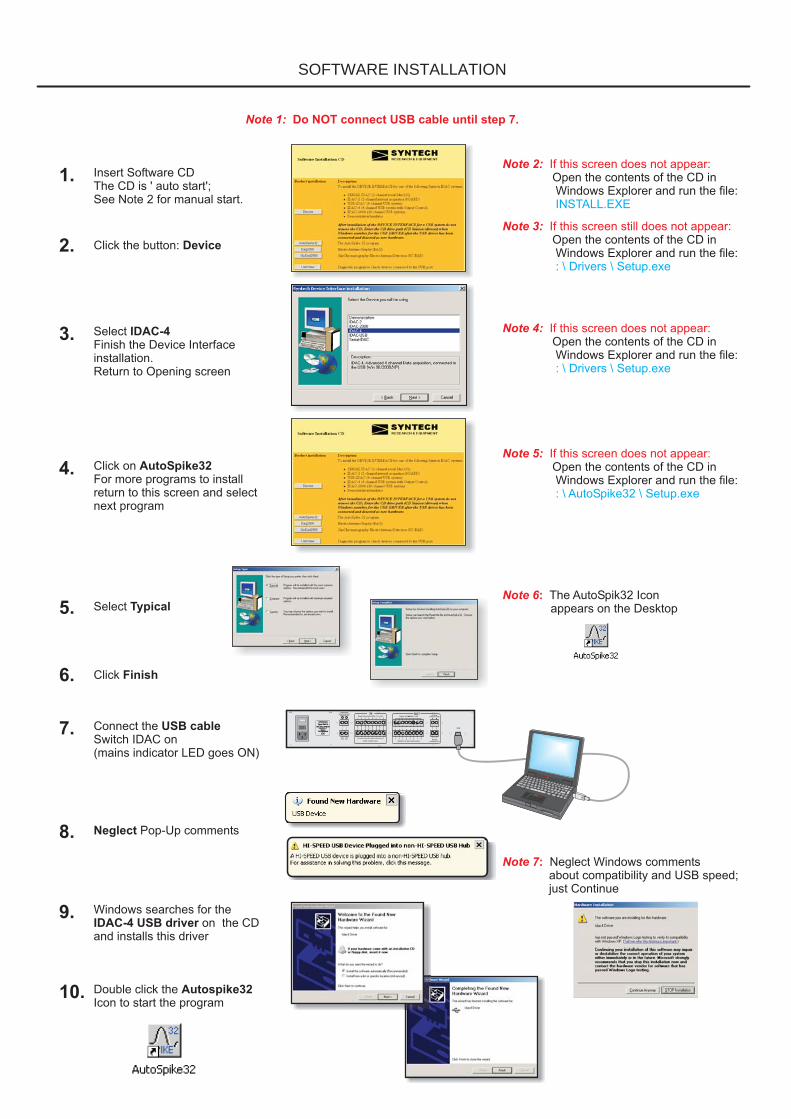
Insert Software CDThe CD is ' auto start';See Note 2 for manual start.
Click the button: Device
SelectFinish the Device Interfaceinstallation.Return to Opening screen
IDAC-4
Click onFor more programs to installreturn to this screen and selectnext program
AutoSpike32
Select Typical
Click Finish
Connect theSwitch IDAC on(mains indicator LED goes ON)
USB cable
Neglect Pop-Up comments
Windows searches for theon the CD
and installs this driverIDAC-4 USB driver
Double click theIcon to start the program
Autospike32
Note 6: The AutoSpik32 Iconappears on the Desktop
Note 7: Neglect Windows commentsabout compatibility and USB speed;just Continue
Note 2: If this screen does not appear:Open the contents of the CD inWindows Explorer and run the file:INSTALL.EXE
Note 1: Do NOT connect USB cable until step 7.
Note 3: If this screen still does not appear:Open the contents of the CD inWindows Explorer and run the file:: \ Drivers \ Setup.exe
Note 4: If this screen does not appear:Open the contents of the CD inWindows Explorer and run the file:: \ Drivers \ Setup.exe
Note 5: If this screen does not appear:Open the contents of the CD inWindows Explorer and run the file:: \ AutoSpike32 \ Setup.exe
1.
SYNTECH
Type: IDAC 4100 - 240 V 50-60 Hz
Fuse 0.5 A, T
Made inThe Netherlands
Made inThe Netherlands
1 2 3 4 5 6 7 8
Input common zeroAnalog
common zero
Digital (Normally HIGH, TTL +5V)
Switches to zero when active
Digital (COMMON + 12V)
Additionalexternal power
(max 24 V) Analog(-10V to +10V)
USB
OUTIN
1 2 3 4 5 6 7 8
1 2 3 4 5 6 7 8 1 2 3 4 5 6 7 8
1 2
1 2
++
+ +
+ +
+ +
++
+ + + + + + + +
+ + + + + + + +
++++++++
+ + + + + + + ++ +
SOFTWARE INSTALLATION
2
INSTALLATION SOFTWARE Note: Install the software BEFORE connecting the IDAC-4 with the USB port! The Syntech software can be used with different Syntech interface devices ( IDAC-4, Serial IDAC, USB-IDAC, IDAC-2 Interface board, IDAC-2000, etc.) For a certain device to operate with the software the appropriate DEVICE INTERFACE must be installed. First install the DEVICE INTERFACE for the IDAC-4, then install the application program (Autospike) followed by connecting the IDAC to the USB port.
DEVICE INTERFACE Installation: 1. Insert program CD ROM ; The CD is " auto-run" ; if the CD does not start
automatically, the installation can be started manually: 2. Manual start: Run the file: INSTALL.exe 3. Click the " Device " button in the Installation Web Page 4. Select " IDAC-4 " in the device selection box. PROGRAM Installation: 5. After the driver has been installed, click the AutoSpike button. 6. Follow the instructions. 7. Select " CUSTOM " in the installation mode selection box 8. After the installation procedure is finished the hardware can be installed. 9. DO NOT REMOVE the CD from the station. After the hardware is connected Windows needs this disk to activate the USB-driver for the newly detected hardware.
INTELLIGENT DATA ACQUISITION CONTROLLER PROGRAMMABLE OUTPUT DRIVERSIDAC 4
3
UNIVERSALSERIAL BUS
1 2
INPUTS / OUTPUTS
DIGITAL INPUTS
DIGITAL IN / OUT
INDICATORS
DIGITAL OUTPUTS
1 12 23 34 45 56 67 78 8
ANALOG
SIGNAL INPUTS
DIGITAL
INPUTS
1 - 4
42 311 2 42
USBcable
PC
MAINS
ACTIVE
AUDIO OUT
+ 12 V- 12 V
- signal
commonGND
NC
(central pin)+ signal
FRONT VIEW
SYNTECH
Type: IDAC 4100 - 240 V 50-60 Hz
Fuse 0.5 A, T
Made inThe Netherlands
Made inThe Netherlands
1 2 3 4 5 6 7 8
Input common zeroAnalog
common zero
Digital (Normally HIGH, TTL +5V)
Switches to zero when active
Digital (COMMON + 12V)
Additionalexternal power
(max 24 V) Analog(-10V to +10V)
USB
OUTIN
1 2 3 4 5 6 7 8
1 2 3 4 5 6 7 8 1 2 3 4 5 6 7 8
1 2
1 2
++
+ +
+ +
+ +
++
+ + + + + + + +
+ + + + + + + +
++++++++
+ + + + + + + ++ +
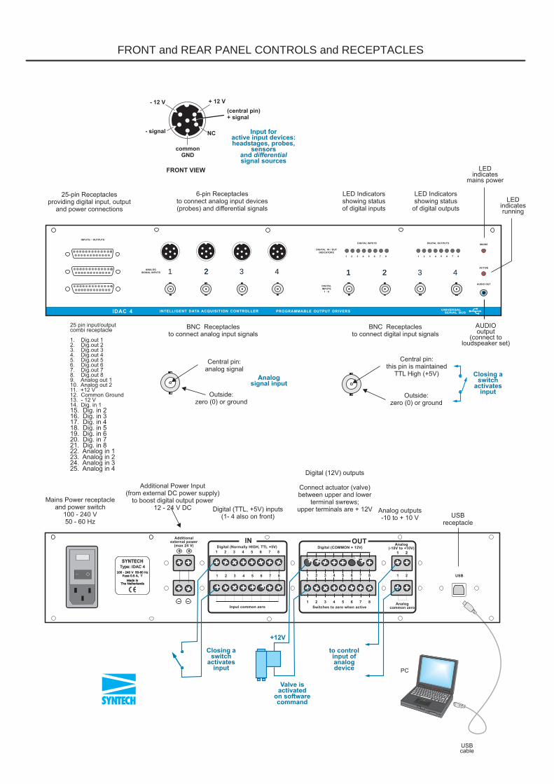
25-pin Receptaclesproviding digital input, output
and power connections
6-pin Receptaclesto connect analog input devices(probes) and differential signals
BNC Receptaclesto connect analog input signals
Mains Power receptacleand power switch
100 - 240 V50 - 60 Hz
Additional Power Input(from external DC power supply)
to boost digital output power12 - 24 V DC Digital (TTL, +5V) inputs
(1- 4 also on front)
Digital (12V) outputs
Connect actuator (valve)between upper and lower
terminal swrews;upper terminals are + 12V Analog outputs
-10 to + 10 V USBreceptacle
Central pin:analog signal
25 pin input/outputcombi receptacle
1. Dig.out 12. Dig.out 23. Dig.out 34. Dig.out 45. Dig.out 56. Dig.out 67. Dig.out 78. Dig.out 89. Analog out 110. Analog out 211. +12 V12. Common Ground13. - 12 V14. Dig. in 115. Dig. in 216. Dig. in 317. Dig. in 418. Dig. in 519. Dig. in 620. Dig. in 721. Dig. in 822. Analog in 123. Analog in 224. Analog in 325. Analog in 4
Central pin:this pin is maintained
TTL High (+5V)
Outside:zero (0) or ground
Outside:zero (0) or ground
Closing aswitch
activatesinput
Closing aswitch
activatesinput
Input foractive input devices:headstages, probes,
sensorsandsignal sources
differential
Analogsignal input
+12V
Valve isactivated
on softwarecommand
to controlinput ofanalogdevice
BNC Receptaclesto connect digital input signals
LED Indicatorsshowing statusof digital inputs
LED Indicatorsshowing status
of digital outputs
LEDindicates
mains power
LEDindicatesrunning
AUDIOoutput
(connect toloudspeaker set)
FRONT and REAR PANEL CONTROLS and RECEPTACLES
3
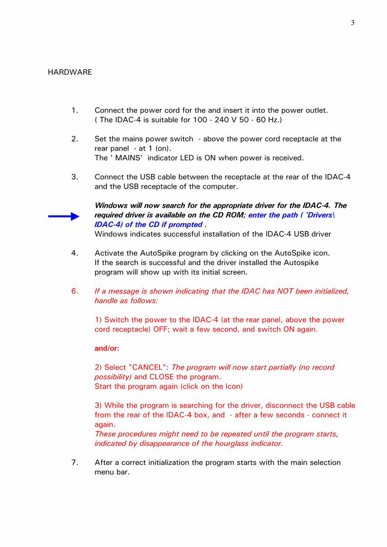
HARDWARE 1. Connect the power cord for the and insert it into the power outlet. ( The IDAC-4 is suitable for 100 - 240 V 50 - 60 Hz.) 2. Set the mains power switch - above the power cord receptacle at the
rear panel - at 1 (on). The ' MAINS' indicator LED is ON when power is received. 3. Connect the USB cable between the receptacle at the rear of the IDAC-4
and the USB receptacle of the computer. Windows will now search for the appropriate driver for the IDAC-4. The
required driver is available on the CD ROM; enter the path ( 'Drivers\ IDAC-4) of the CD if prompted .
Windows indicates successful installation of the IDAC-4 USB driver 4. Activate the AutoSpike program by clicking on the AutoSpike icon. If the search is successful and the driver installed the Autospike
program will show up with its initial screen. 6. If a message is shown indicating that the IDAC has NOT been initialized,
handle as follows: 1) Switch the power to the IDAC-4 (at the rear panel, above the power
cord receptacle) OFF; wait a few second, and switch ON again. and/or: 2) Select "CANCEL": The program will now start partially (no record
possibility) and CLOSE the program. Start the program again (click on the Icon) 3) While the program is searching for the driver, disconnect the USB cable
from the rear of the IDAC-4 box, and - after a few seconds - connect it again.
These procedures might need to be repeated until the program starts, indicated by disappearance of the hourglass indicator.
7. After a correct initialization the program starts with the main selection
menu bar.
4
Note: Installation of the IDAC-4 USB driver can be checked in the Device Manager after opening the Windows SETTING menu - Control Panel - System - Device Manager. In case the driver is not present reboot the computer and activate the AutoSpike program again with the IDAC-4 connected to the USB port and mains power. Some early version of Windows98 may have problems with correct identification and installation of USB hardware drivers. It is recommended to install a recent (aug. 2000 ) Windows98 version or to upgrade to the most recent version. The IDAC-4 does NOT run with APPLE computers, even if they have a USB port, because of incompatibility with the operating system.
SIGNAL CONNECTIONS INPUT SIGNALS Analog Signal sources are connected to the system via the input receptacles at the front of the device. Output signals from amplifiers, tape recorders, signal conditioners, microphones, etc, can be connected directly to the BNC inputs.
Signals picked-up from low voltage, high impedance, low ohm, and other delicate signal sources need to be conditioned by appropriate circuits. For these circuits the 6-pin DIN connectors are intended; they provide the necessary power voltages (+ and - 12V) and a differential signal input.
The resistance of the signal inputs is 1 kOhm. Digital signals, such as trigger commands, event signals, markers, stimulus duration signals, etc. are connected via the four digital input BNC receptacles.
These signals may be either positive (4- 12 V) or negative (a closing switch), and can be momentary (transition from + to zero, or reverse) or continuously, indicating either an onset or offset or a status change (stimulus duration, etc). The 1 - 4 inputs are available on the front panel; all the 8 inputs are also accessible on the rear panel (Digital Inputs) terminals and on the three 25-pin D connectors at the front.
5
OUTPUT SIGNALS
Audio output. To make use of the audio signal output a suitable audio amplifier is needed. A cheap set of loudspeakers with built-in amplifier for computer audio monitoring is fully adequate, and plugs-in directly to the audio output. Some headphones (high impedance types) can be connected directly to the audio output.
Analog signals. Two 12 bit programmable analog signals (-10to +10V V) are delivered from the rear panel output terminals. The signals from these outputs can be programmed dynamically and in synchrony with the signal acquisition. They can be used to control linear actuators, flow controllers. motor speed regulators, light intensity, temperature etc. via appropriate driver circuits. These signals are ' control' voltages; they cannot deliver power. Please consult Syntech at [email protected] for specific information.
Digital signals. 8 digital signals can be accessed from the rear output terminal. The signals can be programmed on the same time base and in synchrony with the signal acquisition for control of actuators like solenoids, valves, lights etc directly without the need for additional interfacing circuits. All inputs and outputs and + - 12V power are also accessible through the 3 connectors (25 sub-D) at the front panel. However, these signals cannot drive actuators directly, as they are only TTL command signals.
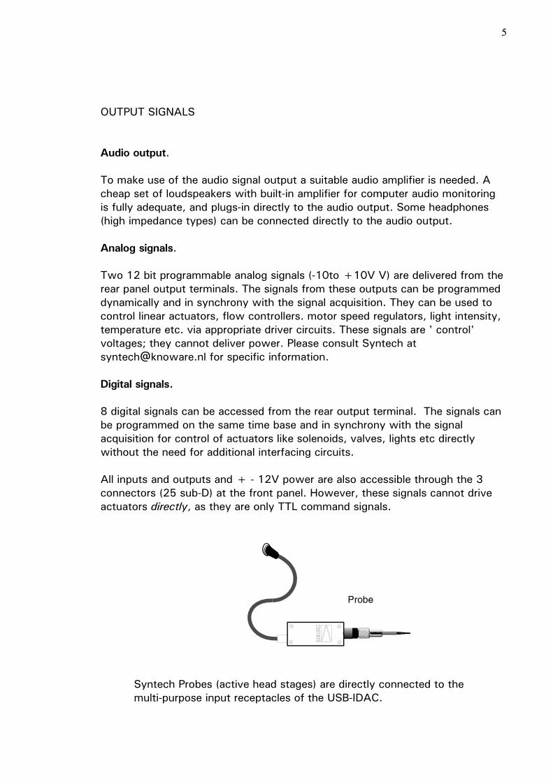
Syntech Probes (active head stages) are directly connected to the multi-purpose input receptacles of the USB-IDAC.
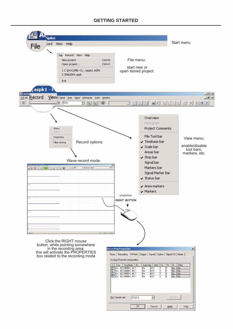
File menu:
start new oropen stored project
Start menu
View menu:
enable/disabletool bars,
markers, etc.
Record options
Click the RIGHT mousebutton, while pointing somewhere
in the recording area;this will activate the PROPERTIESbox related to the recording mode
Wave record mode:
channel 1
channel 2
channel 3
channel 4
digital
GETTING STARTED
properties:
:RIGHT BUTTON

6
OPERATION RECORDING 1) To activate the Recording mode start the AutoSpike program
If the program does not start, a message is presented; click Retry; if the program still does not start switch off the mains (110 or 220V) power to the IDAC-4 (the power switch is located above the power cord receptacle at the rear of the box) OFF and after a few seconds ON again. In most cases the program will start after a few trials.
(If the IDAC-4 is not connected click "cancel"; now the program can be used to operate on saved files; however, recordings cannot be made). Before selecting the Record Mode first enable a few control boxes from the list presented after clicking on View: 2) Click on View It is recommended to activate the following tool bars: * Time base bar * Scale bar * Strip bar * Status bar * Markers 3) Select in the main FILE menu: New project. 4) Click on the menu bar of the aspk1 Project window 5) Click Record 6) Click Wave (Spike recording mod is discussed later) The Wave record window is now activated. This window operates much like a multi-channel oscilloscope: all input signals are displayed on the screen in real-time. Like in an oscilloscope, the Sensitivity (input scale in V or mV), the Time base (writing speed in division/s), DC or AC mode, DC offset, Trigger modes, etc. can be selected or adjusted in control boxes to optimally display and capture the signals. In the Record Control Bar the manual Trigger function, hold and storage buttons, and scale are operated and adjusted. More settings are accessible in the record properties Box, which appears after a Right-Click in the recording area. Filter settings for the signals are adjusted in the 'Filter settings' in the record menu.
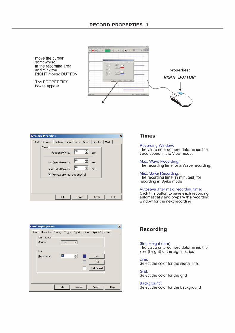
move the cursorsomewherein the recording areaand click theRIGHT mouse BUTTON:
The PROPERTIESboxes appear
Recording Window:
Max. Wave Recording:
Max. Spike Recording
Autosave after max. recording time:
The value entered here determines thetrace speed in the View mode.
The recording time for a Wave recording.
:The recording time (in minutes!) forrecording in Spike mode
Click this button to save each recordingautomatically and prepare the recordingwindow for the next recording
Strip Height (mm):
Line:
Grid:
Background:
The value entered here determines thesize (height) of the signal strips
Select the color for the signal line.
Select the color for the grid
Select the color for the background
Times
Recording
properties:
RIGHT BUTTON:
RECORD PROPERTIES 1
7
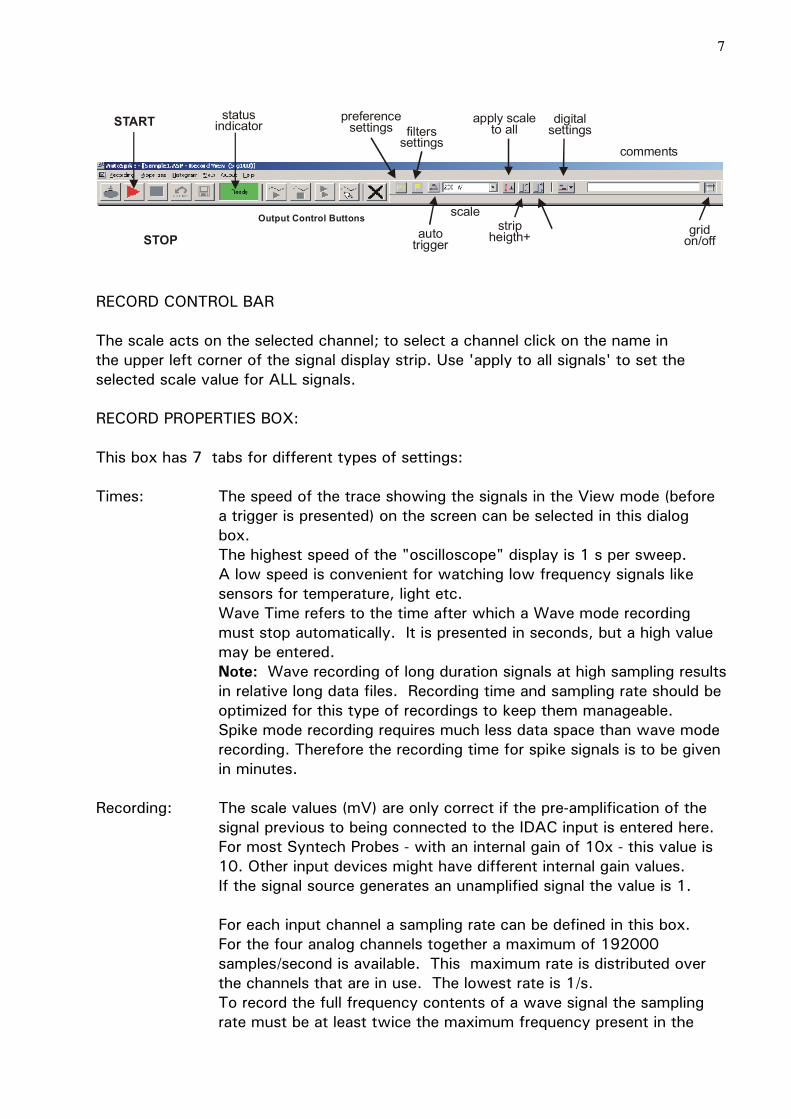
START status
indicator
STOP
preferencesettings
Output Control Buttons
filterssettings
autotrigger
scale
apply scaleto all
digitalsettings
grid on/off
comments
stripheigth+
RECORD CONTROL BAR The scale acts on the selected channel; to select a channel click on the name in the upper left corner of the signal display strip. Use 'apply to all signals' to set the selected scale value for ALL signals. RECORD PROPERTIES BOX: This box has 7 tabs for different types of settings: Times: The speed of the trace showing the signals in the View mode (before
a trigger is presented) on the screen can be selected in this dialog box.
The highest speed of the "oscilloscope" display is 1 s per sweep. A low speed is convenient for watching low frequency signals like sensors for temperature, light etc.
Wave Time refers to the time after which a Wave mode recording must stop automatically. It is presented in seconds, but a high value may be entered.
Note: Wave recording of long duration signals at high sampling results in relative long data files. Recording time and sampling rate should be optimized for this type of recordings to keep them manageable. Spike mode recording requires much less data space than wave mode recording. Therefore the recording time for spike signals is to be given in minutes.
Recording: The scale values (mV) are only correct if the pre-amplification of the
signal previous to being connected to the IDAC input is entered here. For most Syntech Probes - with an internal gain of 10x - this value is 10. Other input devices might have different internal gain values.
If the signal source generates an unamplified signal the value is 1. For each input channel a sampling rate can be defined in this box. For the four analog channels together a maximum of 192000 samples/second is available. This maximum rate is distributed over the channels that are in use. The lowest rate is 1/s.
To record the full frequency contents of a wave signal the sampling rate must be at least twice the maximum frequency present in the
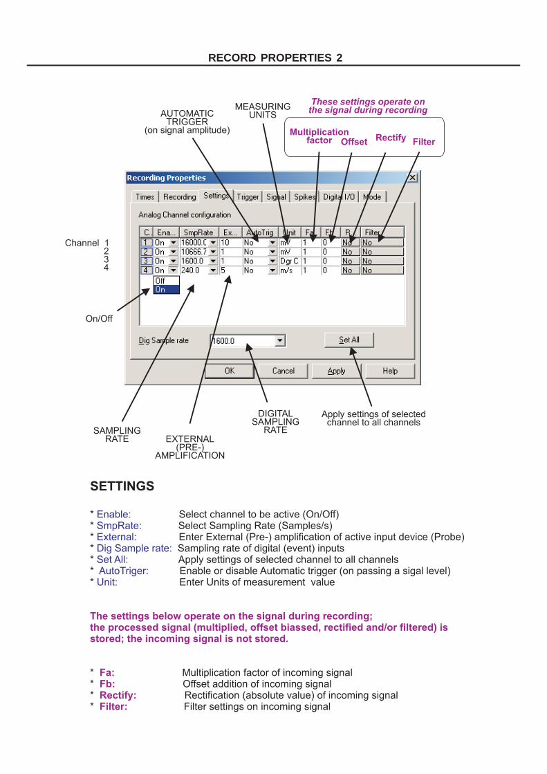
* Select channel to be active (On/Off)* Select Sampling Rate (Samples/s)* Enter External (Pre-) amplification of active input device (Probe)* Sampling rate of digital (event) inputs* Apply settings of selected channel to all channels* Enable or disable Automatic trigger (on passing a sigal level)* Enter Units of measurement value
* Multiplication factor of incoming signal* Offset addition of incoming signal* Rectification (absolute value) of incoming signal* Filter settings on incoming signal
Enable:SmpRate:External:Dig Sample rate:Set All:AutoTriger:Unit:
The settings below operate on the signal during recording;the processed signal (multiplied, offset biassed, rectified and/or filtered) isstored; the incoming signal is not stored.
Fa:Fb:Rectify:Filter:
SETTINGS
On/Off
Channel 1234
SAMPLINGRATE EXTERNAL
(PRE-)AMPLIFICATION
AUTOMATICTRIGGER
(on signal amplitude)
DIGITALSAMPLING
RATE
Apply settings of selectedchannel to all channels
MEASURINGUNITS
Offset
These settings operate onthe signal during recording
Rectify FilterMultiplication
factor
RECORD PROPERTIES 2
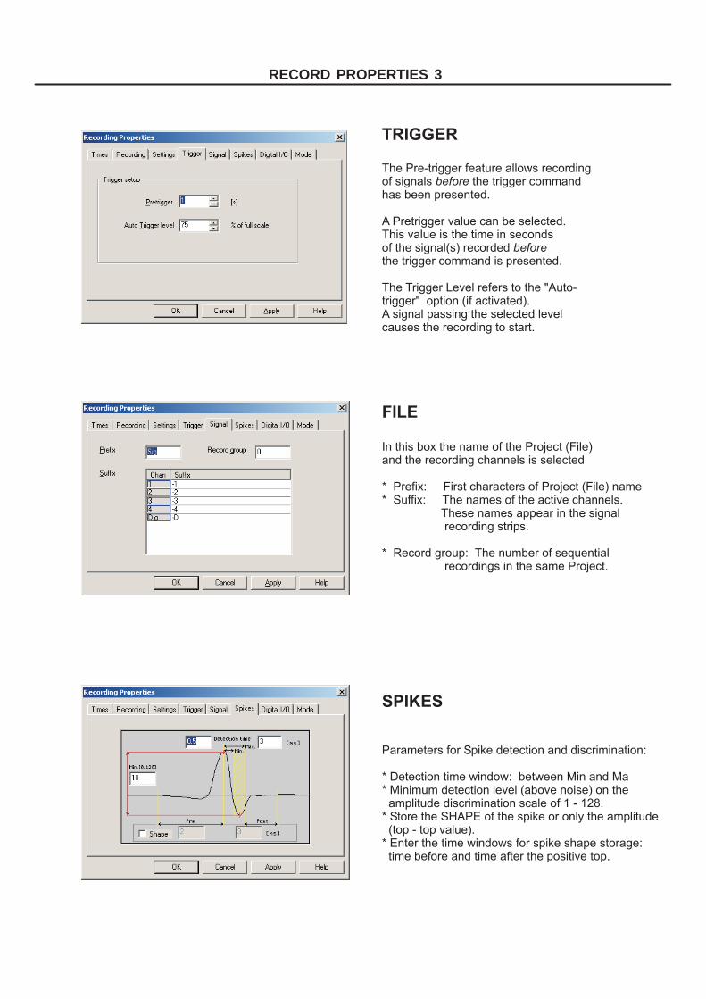
TRIGGER
FILE
SPIKES
The Pre-trigger feature allows recordingof signals the trigger commandhas been presented.
A Pretrigger value can be selected.This value is the time in secondsof the signal(s) recordedthe trigger command is presented.
The Trigger Level refers to the "Auto-trigger" option (if activated).A signal passing the selected levelcauses the recording to start.
before
before
In this box the name of the Project (File)and the recording channels is selected
* Prefix: First characters of Project (File) name* Suffix: The names of the active channels.
These names appear in the signalrecording strips.
* Record group: The number of sequentialrecordings in the same Project.
Parameters for Spike detection and discrimination:
* Detection time window: between Min and Ma* Minimum detection level (above noise) on theamplitude discrimination scale of 1 - 128.
* Store the SHAPE of the spike or only the amplitude(top - top value).
* Enter the time windows for spike shape storage:time before and time after the positive top.
RECORD PROPERTIES 3
RECORD PROPERTIES 4
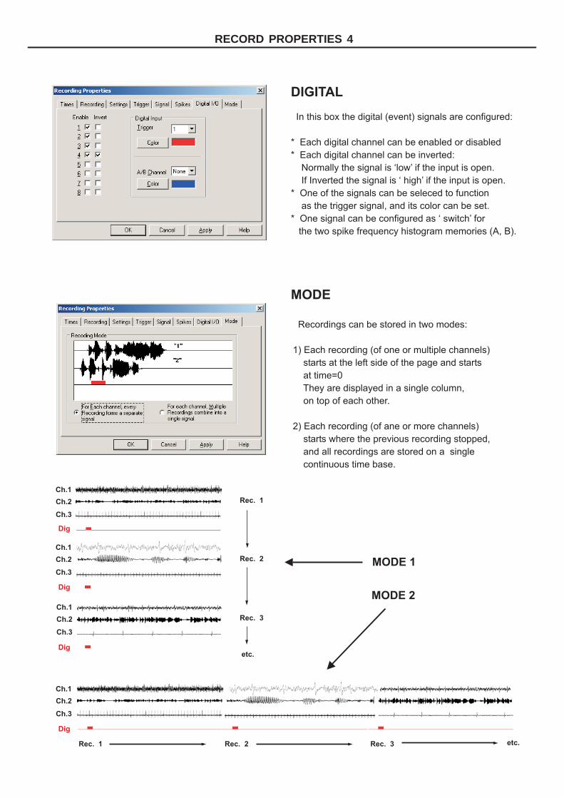
In this box the digital (event) signals are configured:
* Each digital channel can be enabled or disabled
* Each digital channel can be inverted:
Normally the signal is ‘low’ if the input is open.
If Inverted the signal is ‘ high’ if the input is open.
* One of the signals can be seleced to function
as the trigger signal, and its color can be set.
* One signal can be configured as ‘ switch’ for
the two spike frequency histogram memories (A, B).
Recordings can be stored in two modes:
1) Each recording (of one or multiple channels)
starts at the left side of the page and starts
at time=0
They are displayed in a single column,
on top of each other.
2) Each recording (of ane or more channels)
starts where the previous recording stopped,
and all recordings are stored on a single
continuous time base.
DIGITAL
MODE
MODE 1
MODE 2
Ch.1
Ch.1
Ch.1
Ch.1
Ch.2
Rec. 1
etc.
etc.
Rec. 1
Rec. 2
Rec. 2
Rec. 3
Rec. 3
Ch.2
Ch.2
Ch.2
Ch.3
Ch.3
Dig
Dig
Dig
Dig
Ch.3
Ch.3
8
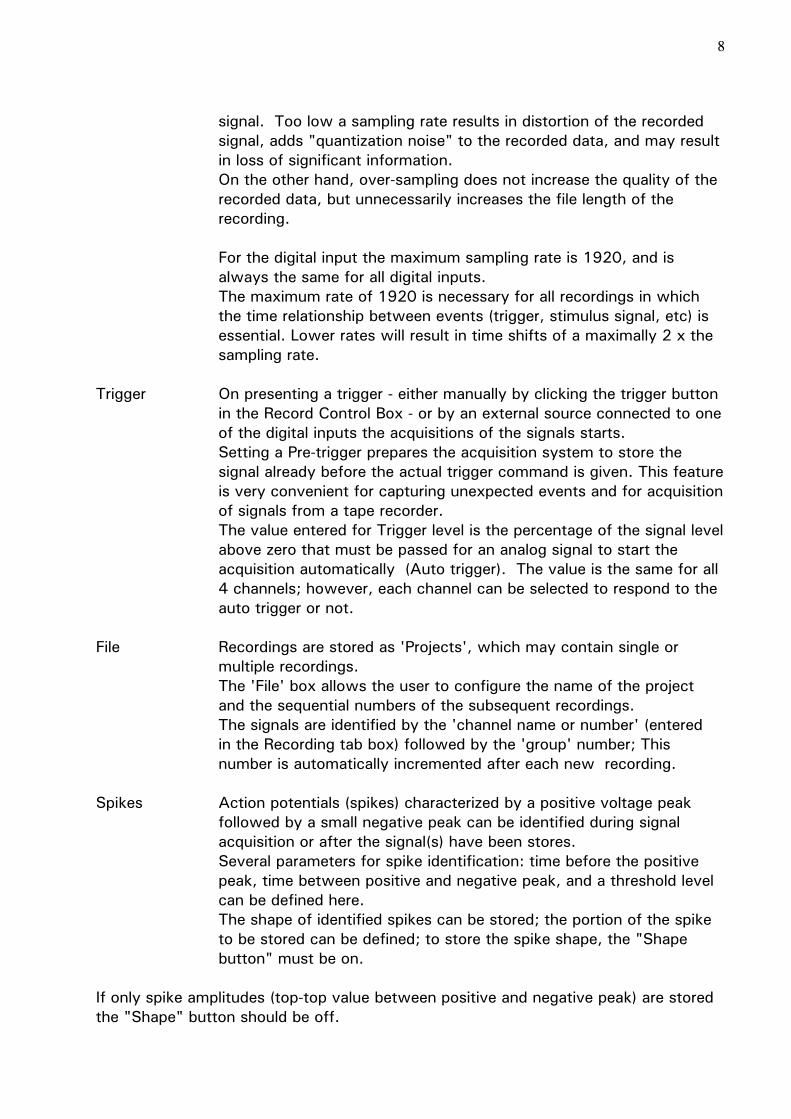
signal. Too low a sampling rate results in distortion of the recorded
signal, adds "quantization noise" to the recorded data, and may result in loss of significant information. On the other hand, over-sampling does not increase the quality of the recorded data, but unnecessarily increases the file length of the recording.
For the digital input the maximum sampling rate is 1920, and is
always the same for all digital inputs. The maximum rate of 1920 is necessary for all recordings in which the time relationship between events (trigger, stimulus signal, etc) is essential. Lower rates will result in time shifts of a maximally 2 x the sampling rate.
Trigger On presenting a trigger - either manually by clicking the trigger button in the Record Control Box - or by an external source connected to one of the digital inputs the acquisitions of the signals starts.
Setting a Pre-trigger prepares the acquisition system to store the signal already before the actual trigger command is given. This feature is very convenient for capturing unexpected events and for acquisition of signals from a tape recorder. The value entered for Trigger level is the percentage of the signal level above zero that must be passed for an analog signal to start the acquisition automatically (Auto trigger). The value is the same for all 4 channels; however, each channel can be selected to respond to the auto trigger or not.
File Recordings are stored as 'Projects', which may contain single or
multiple recordings. The 'File' box allows the user to configure the name of the project and the sequential numbers of the subsequent recordings. The signals are identified by the 'channel name or number' (entered
in the Recording tab box) followed by the 'group' number; This number is automatically incremented after each new recording.
Spikes Action potentials (spikes) characterized by a positive voltage peak followed by a small negative peak can be identified during signal acquisition or after the signal(s) have been stores.
Several parameters for spike identification: time before the positive peak, time between positive and negative peak, and a threshold level can be defined here.
The shape of identified spikes can be stored; the portion of the spike to be stored can be defined; to store the spike shape, the "Shape button" must be on.
If only spike amplitudes (top-top value between positive and negative peak) are stored the "Shape" button should be off.
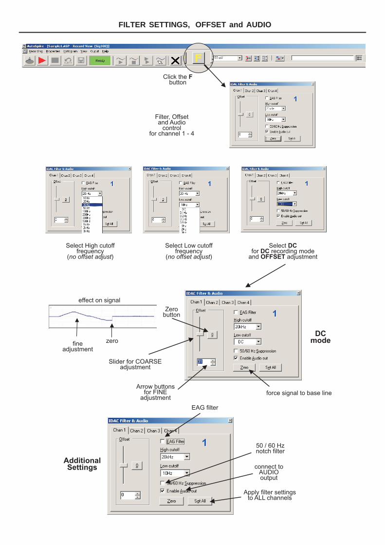
FILTER SETTINGS, OFFSET and AUDIO
Click thebutton
F
Filter, Offsetand Audio
controlfor channel 1 - 4
Select High cutofffrequency
( )no offset adjust
Select Low cutofffrequency
( )no offset adjust
Slider for COARSEadjustment
Zerobutton
zero
effect on signal
fineadjustment
Arrow buttonsfor FINE
adjustment
EAG filter
force signal to base line
Apply filter settingsto ALL channels
50 / 60 Hznotch filter
AdditionalSettings
DCmode
connect toAUDIOoutput
Selectfor recording mode
and adjustment
DCDCOFFSET
9
Digital Two digital input signals can be assigned a special function: 1) to serve as trigger to start the acquisition 2) to switch between Spike Histogram A and B in spike mode recording. The color of these two special signals can be selected.
The polarity of all digital input can be reversed. Normally the input responds to a positive input signal; In reverse the inputs are active during a low input (closed input). The latter configuration is suitable for trigger signals from closing contacts (pedal switch, GC start relay, etc)
Mode Signals can be recorded in two modes: 1) On a common time base; all signals start at time=0 and are stored and displayed on top of each other like lines in a book. 2) On a continuous time base; Each new recording starts where the previous recording ended. The signals are stored and displayed on a ' single line' . FILTER SETTINGS and OFFSET CONTROL Input filters Each analog input channel is provided with programmable analog low
and high pass filters, the settings of which can be adjusted in this box. The purpose of the filters is to condition the signal for proper digitalization by the analog to digital converter in the IDAC. It is important to select the proper filter settings dependent on the kind of information to be derived from the recorded signals.To record information of low frequency character a high pass filter should be set at a low value. For signals containing very low frequencyinformation (like EAGs) the low -pass filter must be set at a low value or at DC. For accurately measuring signal levels, a DC setting is necessary.
In case DC is selected, it is possible to compensate DC offset on the incoming signal using the offset slide bar.
The Zero button (or the Z-key) temporarily overrides the Low pass filter; This button is convenient for Low pass filter settings below 1 Hz, as it results in a quick return to the base line after a large signal transient.
50 or 60 Hz hum induced power line can be suppressed; However, this filter might introduce some offset in the recorded signal.
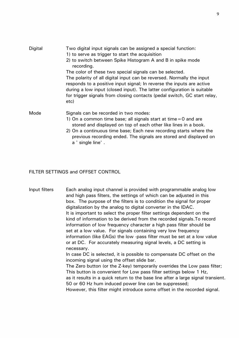
WAVE RECORDING
Channel 1
START
1
2
3
statusindicator
elepsedtime
ENDof recording
STOP
preferencesettings
Output Control Buttons
leaverecording mode
CLEARwithout save
Select recordingsfor display
filterssettings
autotrigger
scale
apply scaleto all
digitalsettings
gridon/off
comments
stripheigth+ strip
heigth-
Channel 2
Channel 3
Channel 4
Digital
10
WAVE FORM RECORDING Wave recording is the standard signal acquisition mode of the IDAC-4. Up to four analog signals and eight digital (command) signals can be recorded simultaneously. All signals are presented in an oscilloscope-like appearance on the monitor screen. Activate Wave recording: 1) Start the Autospike program 2) Click on File in the main menu 3) Select New Project 4) Click on Record 5) Select Wave The Wave Record Window now appears.
In case no signal sources are connected to the inputs the window shows horizontal lines in the center the display area running from left to right. The center of the display area represents the zero level of the inputs signal. Negative voltage fluctuations are indicated by the line moving down, positive by upward deflections. After the signal sources are connected the display of the signals can be adjusted using the record control box and the recording properties (Pre-trigger, Filter and Offset adjustments) should be selected.
If less than 4 signals are recorded, the non-used channels can be disabled. Start Acquisition: 1) Using the Trigger button in the record control box: Give a left mouse click on the Trigger button. 2) By means of an external (closing switch) signal: Connect a (pedal) switch to the digital input that is configured as trigger input and press the pedal. 3) From stimulus device producing a positive voltage output: Connect this output to one of the digital inputs, configure this input as trigger, and set its polarity to inverse. 4) By the analog signal it self when passing a (positive) threshold: Enable the Auto trigger for that channel and adjust the threshold in the trigger Properties. In addition connect a pedal switch to the digital input, which is configured as trigger input.
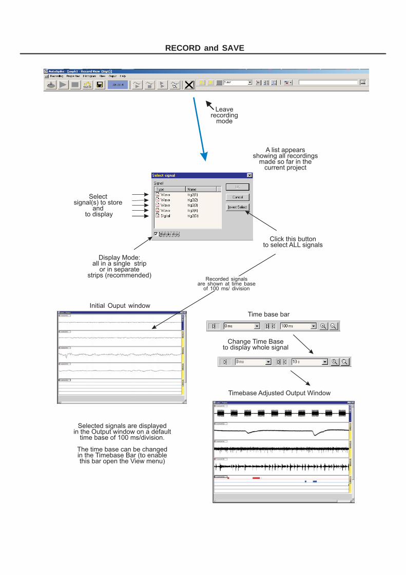
Selectsignal(s) to store
andto display
A list appearsshowing all recordings
made so far in thecurrent project
Display Mode:all in a single strip
or in separatestrips (recommended)
Click this buttonto select ALL signals
Selected signals are displayedin the Output window on a default
time base of 100 ms/division.
The time base can be changedin the Timebase Bar (to enablethis bar open the View menu)
Time base bar
Timebase Adjusted Output Window
Initial Ouput window
Change Time Baseto display whole signal
Recorded signalsare shown at time base
of 100 ms/ division
RECORD and SAVE
Leaverecording
mode
11
The auto trigger is hold-up (to avoid false triggering during pre- adjustment of the signal) until a command is given by the pedal switch. This ' wait status' is indicated by the status indicator. Stop acquisition: 1) Manually: Click the Pause button in the record control box. 2) Automatically: Wait until the pre-set recording time is elapsed. Continue acquisition: 1) Click the Pause button again. Erase and Redo: Click the Clear button; this erases the previous recording from memory and prepares the system for the next acquisition. Save recording(s): Click the Save button, and leave the Record mode. A Selection window appears showing a list of all signals recorded during the last acquisition. The signals are named and numbered according to the settings in File. Display options: Time base: Use the time base numerical scroll windows or the 'Enlarge- Reduce' buttons. Note: All signals are presented on one and the same time base; within a project the time base cannot be adjusted differently for different signals. To display and operate on a different time base the project must be saved under another name and opened as a new project. Multiple projects can be managed simultaneously under Windows, and informatio can be transferred via the clipboard. Scrolling: Use the horizontal scroll bar of the Output window. Amplitude: The amplitude of each signal can be changed; 1) Select the signal by clicking the Name Box (the edge of the box is highlighted) 2) Change the mV value in the Scale bar; intermediate values may be entered. Strip height: Use the + and - buttons in the Strip bar. Or enter a value in the Strip properties.
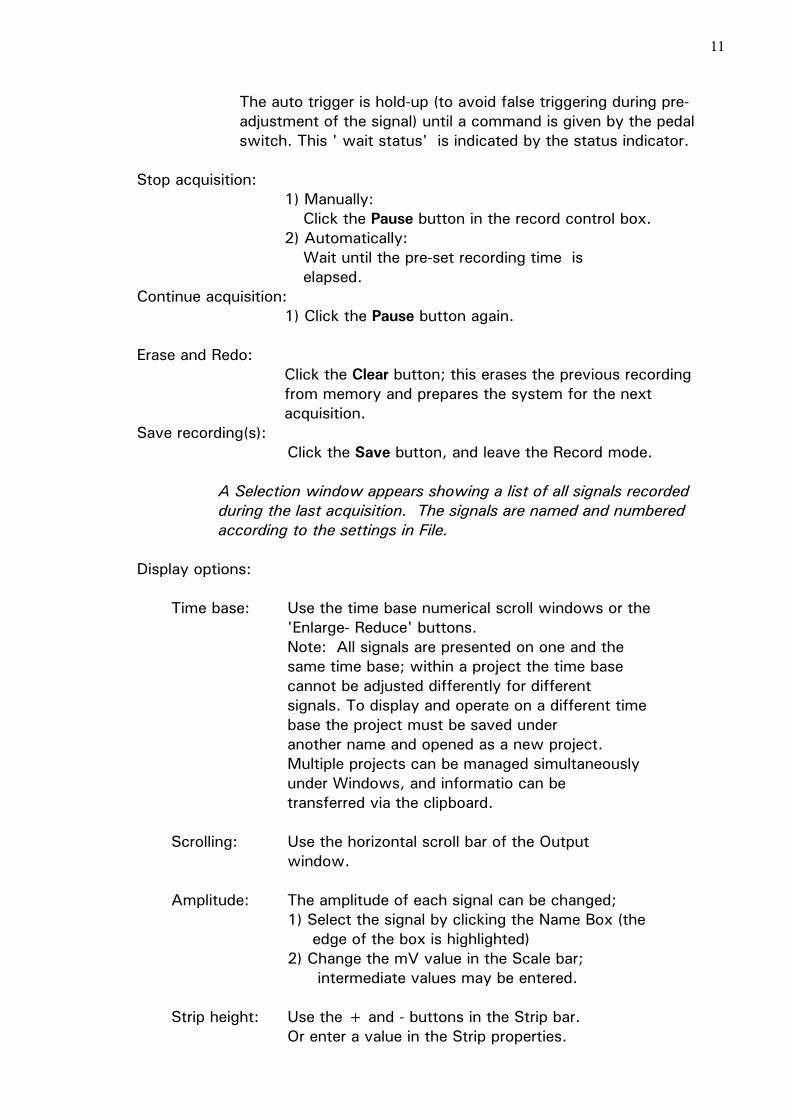
Time base:Operates on ALL strips
Scroll bar
Scroll bar
Operates on the selected strip.Tab boxes to change colors,
grids, scale indications,styles.
Default values can be assignedto all strips by selecting:"Set all strips to default"
Strip properties:
Size:Increase +decrease -
Scale:Increase +decrease -
Timebase:Increase +decrease -
Strip bar:Operates on ALL strips:change size, properties,
grid, scale. etc.
to select Signal:Click on Name box
Scale:Operates on
Selected Signal only
properties:
:RIGHT BUTTON
DISPLAY and OPERATE 1
12
Strip Scroll: Use the right-side scroll bar of the Output Window. The number of currently visible and
non-visible strips is indicated in the Status bar enabling in the View menu.
Strips: The output window is organized in strips, in which
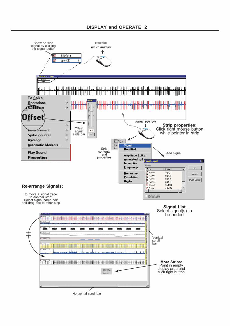
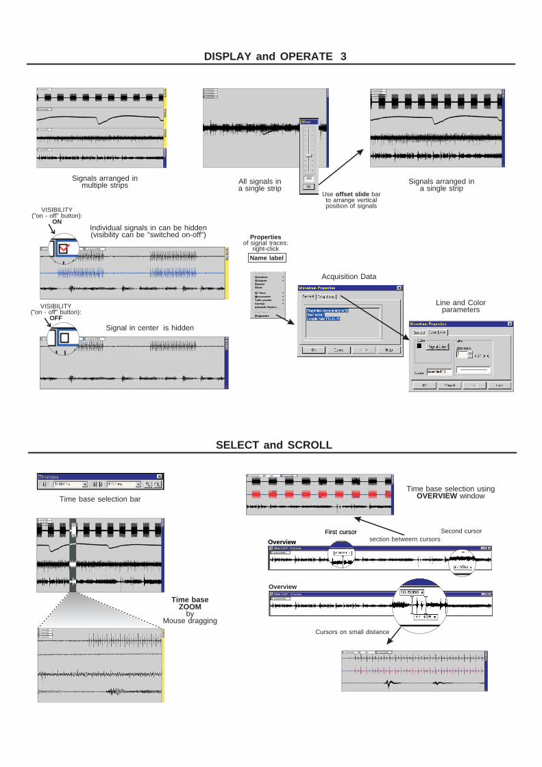
the signals are displayed. Signals can be arranged in a single strip or distributed over as many strips as needed. The properties of strips (background color, grid, scales, etc.) can be defined individually for each strip, or as default for all strips. Signal properties (line thickness and color) are adjustable for each individual signal and are independent of the strip settings. Right- Click the Name Box of the signal to access the signal properties. Grid and Scale: A right mouse click in the strip area presents the strip properties box, in which the characteristics for the selected strip can be adjusted. Signal data: Acquisition settings for a signal are shown in the properties box appearing by right-clicking the signal's name box: 1) Signal Name 2) Rec. Factor (= ext. amplification) 3) Sampling rate Offset : Signals can be individually moved up and down in the strip display field using the offset slide bar. The offset slide bar appears after a Right -Click on the signal Name Box followed by selecting Offset. Depending upon how signals are related they can be arranged all in a single strip or grouped into different stripes, each with their own background, grid and scale settings. Overview: The overview (to enable in the View menu) is aimed to show the full recording period. To add signals to this window give a Right -click inside its display field
end select a signal from the list. Two cursors, each linked to a box showing the time position, can be moved together or relative to each other. They allow fine and numerical selecting of any time base section. It is convenient to downsize the overview window into a strip below the output view.
properties:
:RIGHT BUTTON
:RIGHT BUTTON
Click right mouse buttonwhile pointer in strip
Strip properties:
Select signal(s) tobe added
Signal List
Point in emptydisplay area andclick right button
More Strips:
Re-arrange Signals:
Show or Hidesignal by clickingthe signal button
to move a signal traceto another strip:
Select signal name boxand drag box to other strip
Offsetadjust
slide bar
Stripcontents
andproperties
Horizontal scroll bar
Verticalscrollbar
Add signal
DISPLAY and OPERATE 2
DISPLAY and OPERATE 3
SELECT and SCROLL
byMouse dragging
Time baseZOOM
All signals ina single strip
Time base selection usingwindowOVERVIEWTime base selection bar
Individual signals in can be hidden(visibility can be "switched on-off")
Signal in center is hidden
of signal traces:right-click
Properties
Use barto arrange verticalposition of signals
offset slide
First cursorFirst cursor Second cursor
OverviewOverview
Overview
section betweern cursors
Cursors on small distance
VISIBILITY("on - off" button):
ON
VISIBILITY("on - off" button):
OFF
Signals arranged ina single strip
Acquisition Data
Line and Colorparameters
Signals arranged inmultiple strips
Name label

Openof signal by right-clicking
the
Properties
NAME BOX
Amplitude HISTOGRAM
Useto change colors,line thickness, etcof Spike signal.
Select a colorfor " OUT of Range"
and a colorfor " Selected" spikes
Properties
weak
prominent
:number of spikes
counted inamplitude classes
(1-127)
Vertical scale
amplitudespikes selected
in histogramusing selection bar
SMALL
LARGE amplitudespikes selected
in histogramusing selection bar
SMALL (blueamplitude spikes selected ; out of range: grey)
LARGE (blueamplitude spikes selected ; out of range: grey)
: Amplitude classes (1-127)Horizontal scale
The is presented on top ofthe Wave signal trace immediately after conversion.
The Wave can be " switched off" to show the Spike signal only
SPIKE trace
dialog boxappears
Convert Wave to Spike
Spike selection barSelectedSpikes
selectTo Spike
toptime limitPre-
toppart
Pre-
Detection Time window
storage windowSHAPE
Detection
(on scaleof 128 points)
THRESHOLD
Click this buttonto the
of the spikes
storeSHAPE
click forSpike Amplitude
Histogram
noise smallspikes
smallspikes
smallspikes
largespikes
largespikes
largespikes
-toptime limitPost
-toppart
Post
SPIKE DISCRIMINATION and SELECTION
13
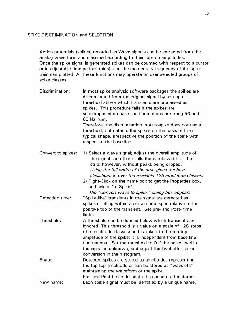
SPIKE DISCRIMINATION and SELECTION Action potentials (spikes) recorded as Wave signals can be extracted from the analog wave form and classified according to their top-top amplitudes.
Once the spike signal is generated spikes can be counted with respect to a cursor or in adjustable time periods (bins), and the momentary frequency of the spike train can plotted. All these functions may operate on user selected groups of spike classes.
Discrimination: In most spike analysis software packages the spikes are discriminated from the original signal by setting a threshold above which transients are processed as spikes. This procedure fails if the spikes are superimposed on base line fluctuations or strong 50 and 60 Hz hum. Therefore, the discrimination in Autospike does not use a threshold, but detects the spikes on the basis of their typical shape, irrespective the position of the spike with respect to the base line. Convert to spikes: 1) Select a wave signal; adjust the overall amplitude of the signal such that it fills the whole width of the strip; however, without peaks being clipped. Using the full width of the strip gives the best classification over the available 128 amplitude classes. 2) Right-Click on the name box to get the Properties box, and select "to Spike". The "Convert wave to spike " dialog box appears. Detection time: "Spike-like" transients in the signal are detected as spikes if falling within a certain time span relative to the positive top of the transient. Set pre- and Post- time limits. Threshold: A threshold can be defined below which transients are ignored. This threshold is a value on a scale of 128 steps (the amplitude classes) and is linked to the top-top amplitude of the spike; it is independent from base line fluctuations. Set the threshold to 0 if the noise level in the signal is unknown, and adjust the level after spike conversion in the histogram. Shape: Detected spikes are stored as amplitudes representing the top-top amplitude or can be stored as "wavelets" maintaining the waveform of the spike. Pre- and Post times delineate the section to be stored. New name: Each spike signal must be identified by a unique name.
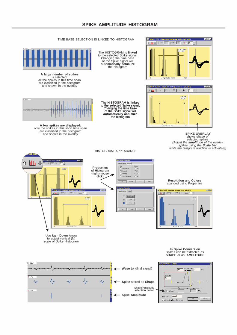
The HISTOGRAM isto the selected Spike signal;
Changing the time baseof the Spike signal will
the histogram
linked
automatically actualize
TIME BASE SELECTION IS LINKED TO HISTOGRAM
HISTOGRAM APPEARANCE
shows shape ofselected spikes
SPIKE OVERLAY
(Adjust the of the overlayspikes using the
while the Histgram windfow is activated))
amplitudeScale bar
is selected:all the spikes in this time spanare classified in the histogram
and shown in the overlay
A large number of spikes
only the spikes in this short time spanare classified in the histogram
and shown in the overlay
A few spikes are displayed:
The HISTOGRAM isto the selected Spike signal;
Changing the time baseof the Spike signal will
the histogram
linked
automatically actualize
The HISTOGRAM isto the selected Spike signal;
Changing the time baseof the Spike signal will
the histogram
linked
automatically actualize
Use Arrowto adjust vertical (N)
scale of Spike Histogram
Up - Down
Inspikes can be extracted as
or as
Spike Conversion
SHAPE AMPLITUDE
andacanged using PropertiesResolution Colors
Shape/Amplitudebuttonselection
(original signal)Wave
stored asSpike Shape
Spike Amplitude
of Histogram(right-mouse
click)
Properties
SPIKE AMPLITUDE HISTOGRAM
14
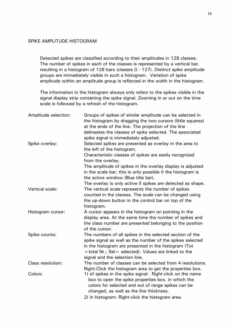
SPIKE AMPLITUDE HISTOGRAM Detected spikes are classified according to their amplitudes in 128 classes. The number of spikes in each of the classes is represented by a vertical bar, resulting in a histogram of 128 bars (classes 0 - 127). Distinct spike amplitude groups are immediately visible in such a histogram. Variation of spike amplitude within an amplitude group is reflected in the width in the histogram.
The information in the histogram always only refers to the spikes visible in the signal display strip containing the spike signal. Zooming in or out on the time scale is followed by a refresh of the histogram.
Amplitude selection: Groups of spikes of similar amplitude can be selected in the histogram by dragging the two cursors (little squares) at the ends of the line. The projection of the line delineates the classes of spike selected. The associated spike signal is immediately adjusted. Spike overlay: Selected spikes are presented as overlay in the area to the left of the histogram. Characteristic classes of spikes are easily recognized from the overlay. The amplitude of spikes in the overlay display is adjusted in the scale bar; this is only possible if the histogram is the active window (Blue title bar). The overlay is only active if spikes are detected as shape. Vertical scale: The vertical scale represents the number of spikes counted in the classes. The scale can be changed using the up-down button in the control bar on top of the histogram. Histogram cursor: A cursor appears in the histogram on pointing in the display area. At the same time the number of spikes and the class number are presented belonging to the position of the cursor. Spike counts: The numbers of all spikes in the selected section of the spike signal as well as the number of the spikes selected in the histogram are presented in the histogram (Tot =total Nr.; Sel= selected). Values are linked to the signal and the selection line. Class resolution: The number of classes can be selected from 4 resolutions. Right-Click the histogram area to get the properties box. Colors: 1) of spikes in the spike signal: Right-click on the name box to open the spike properties box, in which the
colors for selected and out of range spikes can be changed, as well as the line thickness.
2) in histogram: Right-click the histogram area.
Select Spike signal strip
A appears;move the cursor to the position
from where spikes must becounted
CURSOR
Open the Properties boxto the valuesthe for transfer
in other programs
transfer toclipboard
Each cursor presents:
and counts.of
spike counts can betransferred individually
or togetherto the
3 values
Numerical values
clipboard
pre-, post,difference
outputof all spike counts
transferred toWindows Excel
via the
Numerical
clipboard
A Right-Mouse clickopens a Property box
on the cursor
Spikes can be countedon any position in the signalwhere a spike counter cursor
is placed.Spikes are counted before
and after the cursor.
counting periodscan be set in the
of the cursor,which is presented on a
Pre- and Post time
Properties
right-mouse clickon the cursor
counting periodsare entered in ms;
default values can be setor the values can be set for each
individual cursor
Pre- and Post time
Select:Spike counter
Select:Add
Name Time (ms) pre-t pre-N post-N diff. Npost-t
spk1 6777.2 200 500 14 36 22
7633.5 100 300 0 29 29
8710.8 100 200 6 20 14
9074.4 50 100 5 7 2
9792.6 200 500 14 36 22
10829 50 200 5 20 15
Open Properties(right click on Name Box)
a Spike counter cursor is placed
Spike counter cursor
clickhere
Spike signal trace showing multiple spike counter cursors placed
SPIKE COUNTER
15
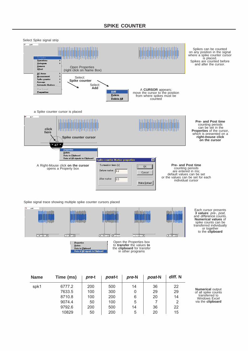
SPIKE COUNTER Spikes can be counted interactively using spike count markers, which are placed in the spike signal trace. The time sections before and after the central cursor of the markers are user defined for all markers or for each marker individually. Spikes are counted before and after cursor and the difference is calculated. The numerical values can be transferred via the clipboard to other applications such as Windows Excel. Add spike counter: 1) Select a spike signal 2) Right-click on the name box 3) Select Spike counter 4) Select Add A marker appears in the spike signal strip. Use the mouse to drag (left button down) the marker into position 5) Release the left mouse button to fix the marker A marker can always be re-positioned by selecting the central cursor by a right mouse click followed by dragging. Counter properties: 1) Select the marker 2) Right-click the central cursor 3) Select properties The counter properties box appears 4) Enter the Pre- and Post- marker times 5) Click OK The values refer to the selected marker only, unless the box "Make default" is selected. Number of markers: An unlimited number of markers can be positioned in a single or multiple signals. Each marker may be assigned its own counting times. Delete markers: Counting markers are deleted individually or all using the command in the properties box appearing after a right- click on the central cursor. Data transfer: Data of all or individual counters are transferred to the clipboard using the appropriate command in the properties box appearing after a right-click on the central cursor.
Convert Wave to Spike
Frequency bar graph of andspk4(2) (Blue) spk4 (Red)
The barautomaticallychanges to when
Frequency is selected
SCALEHz
Hz
size adjustedBIN mode displayLINE filter applied on lineSMOOTH
Frequency bar graph of and (invisible)spk4(2) (visible) spk4
Open of Frequency signal (Right-Click in Name Box)Properties
Right-Clickto create new strip
Use HISTOGRAM to select spikes; Move Spike signal to empty strip
Rihgt-Click the stripto open the box.
SelectSelect
InsertSignal
Frequency
Use
in multiplefrequencydisplay,or use
display
colorcontrast
multiple strip
Open
to add/select
etc.
Strip Properties
GRID,SCALE
Useof selected graphto change display
parameters:
width,Graph,curve
thickness,filter,
Properties
BinBarLine
LineSmooth
Colors
A of recorded andconverted signals appears.
the Spike signalfor the Frequency plot;
signalscan be selected
List
Select
Multiple
After a signal has beenconverted to a signalthe momentary frequency of
the spike signal can be presentedin a plot or curve.
The Frequency plot is basedon the spikes.
Changing the selection inthe automatically
adjusts the Frequency plot
WaveSpike
Frequency
selected
HISTOGRAM
SPIKE FREQUENCY
16
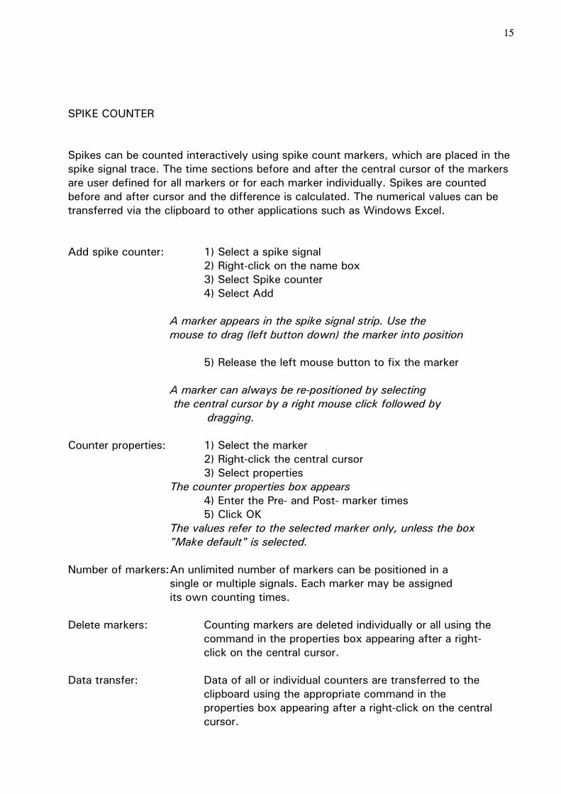
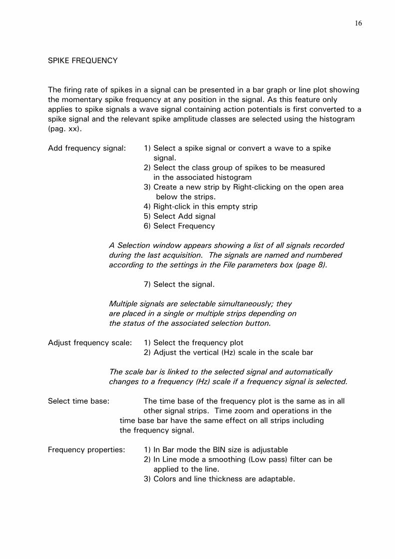
SPIKE FREQUENCY The firing rate of spikes in a signal can be presented in a bar graph or line plot showing the momentary spike frequency at any position in the signal. As this feature only applies to spike signals a wave signal containing action potentials is first converted to a spike signal and the relevant spike amplitude classes are selected using the histogram (pag. xx). Add frequency signal: 1) Select a spike signal or convert a wave to a spike signal. 2) Select the class group of spikes to be measured in the associated histogram 3) Create a new strip by Right-clicking on the open area below the strips. 4) Right-click in this empty strip 5) Select Add signal 6) Select Frequency A Selection window appears showing a list of all signals recorded during the last acquisition. The signals are named and numbered according to the settings in the File parameters box (page 8). 7) Select the signal. Multiple signals are selectable simultaneously; they are placed in a single or multiple strips depending on the status of the associated selection button. Adjust frequency scale: 1) Select the frequency plot 2) Adjust the vertical (Hz) scale in the scale bar The scale bar is linked to the selected signal and automatically changes to a frequency (Hz) scale if a frequency signal is selected. Select time base: The time base of the frequency plot is the same as in all other signal strips. Time zoom and operations in the time base bar have the same effect on all strips including the frequency signal. Frequency properties: 1) In Bar mode the BIN size is adjustable 2) In Line mode a smoothing (Low pass) filter can be applied to the line. 3) Colors and line thickness are adaptable.
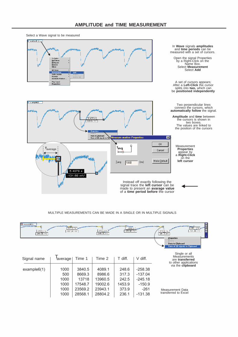
Select a Wave signal to be measured
MULTIPLE MEASUREMENTS CAN BE MADE IN A SINGLE OR IN MULTIPLE SIGNALS
A set of cursors appears;After a the cursor
splits into which canbe
Left-Clicktwo,
positioned independently
Measurement
appear bya
on the
Properties
Right-Click
left cursor
Single or allMeasurementsare
to other applicationsvia the
transferred
clipboard
Measurement Datatransferred to Excel
Signal name Taverage Time 1 Time 2 T diff. V diff.
Instead off exactly following thesignal trace the can bemade to present anof a the cursor
left cursoravarage value
time period before
Two perpendicular linesconnect the cursors, which
the signal.
and betweenthe cursors is shown in
two boxes.The values are linked to
the position of the cursors
automatically follow
Amplitude time
In signalsand can be
measured with a set of cursors.
Open the signal Propertiesby a Right-Click on the
Name Box.Select
Select
Wave amplitudestime periods
MeasurementAdd
example6(1) 1000 3840.5 4089.1 248.6 -258.38
500 8669.3 8986.6 317.3 -137.04
1000 13718 13960.5 242.5 -245.18
1000 17548.7 19002.6 1453.9 -150.9
1000 23569.2 23943.1 373.9 -261
1000 28568.1 28804.2 236.1 -131.38
averageT
AMPLITUDE and TIME MEASUREMENT

17
AMPLITUDE and TIME MEASUREMENT In wave form signals amplitude and time differences can interactively be measured by means of a pair of cursors, which are placed anywhere on the signal. A many of these cursor pairs can be placed as needed and the numerical data can be transferred to the clipboard. Add measurement: 1) Select the strip and the signal of interest The measurement option applies to wave signals only. 2) Right-click on the name box to open a selection box 3) Select Measurement 4) Select Add A pair of cursors appears. Each cursor can be moved along the time base axis and automatically follows the signal trace. The time between the cursors and the voltage differences are numerically presented in two boxes associated with the cursors. Zoom-in for more detail and enlarge the strip. Average option: In many measurements it is advantageous for the first
position point (cursor) to represent an average of the foregoing signal rather than the exact momentary value. For this purpose the first cursor can be assigned a certain time span over which the average signal value is calculated.
Average time: 1) Right-click the first (left) cursor. 2) Select Properties 3) Enter an average time in ms. The value refers to the selected cursor only, unless the box "Make default" is selected. Number of markers: An unlimited number of measurement markers can be positioned in a single or multiple signals. Each marker may be assigned its own counting times. Delete markers: Measurement markers are deleted individually or all using the command in the properties box appearing after a right-click on the left cursor. Data transfer: Data of all or individual markers are transferred to the clipboard using the appropriate command in the properties box appearing after a right-click on the left cursor.
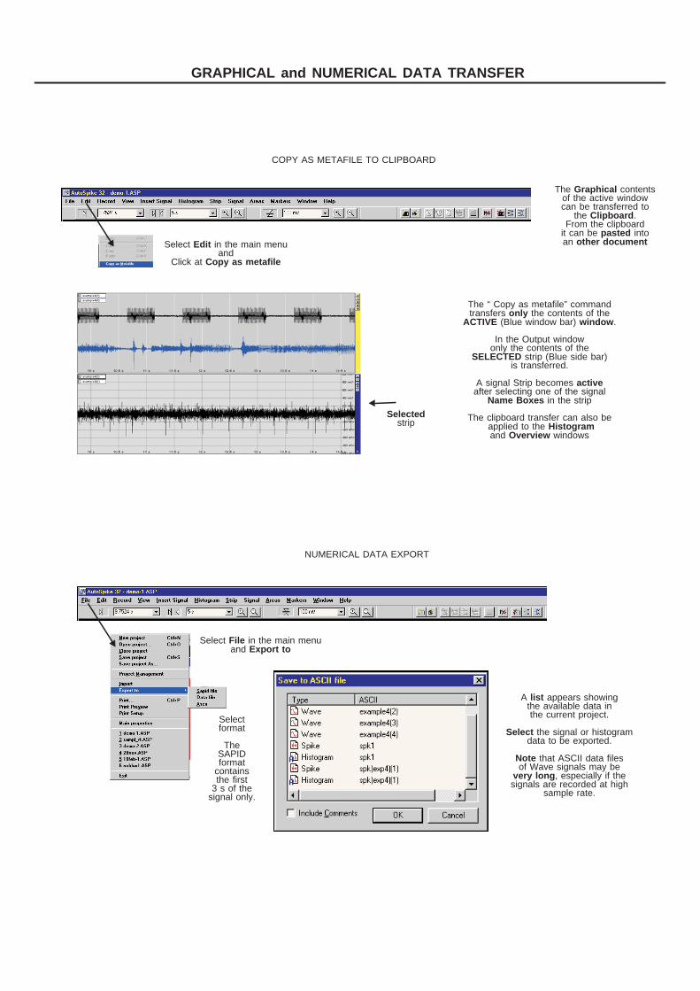
COPY AS METAFILE TO CLIPBOARD
NUMERICAL DATA EXPORT
The contentsof the active windowcan be transferred to
the .From the clipboard
it can be intoan
Graphical
Clipboard
pastedother document
A appears showingthe available data inthe current project.
the signal or histogramdata to be exported.
that ASCII data filesof Wave signals may be
, especially if thesignals are recorded at high
sample rate.
list
Select
Note
very long
Select in the main menuand
Click at
Edit
Copy as metafile
Select in the main menuandFile
Export to
Selectformat
TheSAPIDformat
containsthe first
3 s of thesignal only.
Selectedstrip
The “ Copy as metafile” commandtransfers the contents of the
(Blue window bar) .
In the Output windowonly the contents of the
strip (Blue side bar)is transferred.
A signal Strip becomesafter selecting one of the signal
in the strip
The clipboard transfer can also beapplied to theand windows
onlyACTIVE window
SELECTED
active
Name Boxes
HistogramOverview
GRAPHICAL and NUMERICAL DATA TRANSFER
18
GRAPHICAL and NUMERICAL DATA TRANSFER The information of most output windows can be directly transferred into other applications in windows metafile format using the Windows clipboard function. Alternatively, the complete graphical output or a part of it can be printed using the Print and the Print Preview commands in the File menu. The metafile transfer feature is very convenient if graphs have to be pasted into
a text report or assembled together for a presentation. The numerical values of measurements and spike counts can be pasted directly into spreadsheet packages like Windows Excel for further processing.
Metafile properties: 1) Select Main properties in the File menu 2) Select the Metafile tab 3) Include or exclude the Signal legend (=name box) to be copied with the metafile. Strip contents copy: 1) Add signals to a strip or select them using the visibility button (page 11), and adjust the scale and appearance parameters. Only the selected strip (Blue side bar) will be copied to the clipboard 2) Click Edit in the main menu bar 3) Click Copy as Metafile 4) Open the target application 5) Use the Paste command to insert the metafile into the application. Numerical data: A) Measurement and Spike counter values (pag. xx) are transferred to the clipboard using commands linked to the left cursor. B) Histogram and Signal numerical data: 1) Select Export to in the File menu 2) Select one of the export formats 3) Select the Histogram or signal from the list .
SAPID files are in 16 bit format and contain the first 3 seconds of the recording only.
ASCII files may become very large for signals recorded at high sampling rate during (relative) long periods.
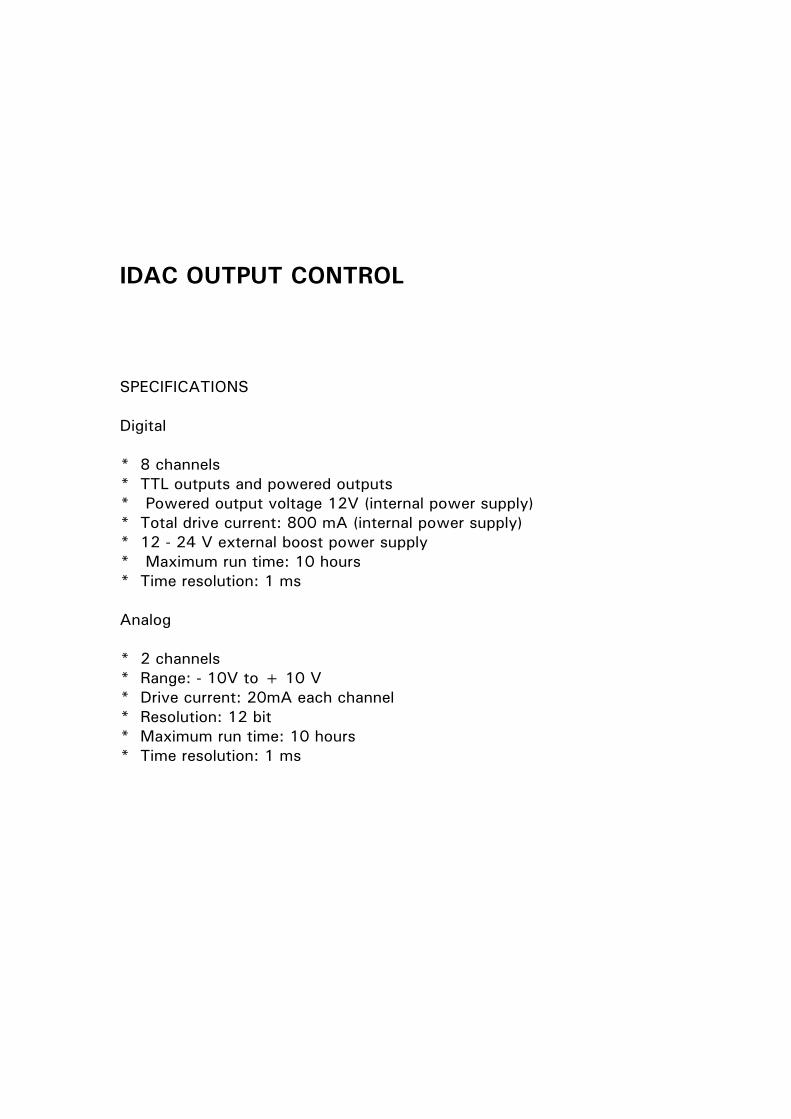
IDAC OUTPUT CONTROL SPECIFICATIONS Digital * 8 channels * TTL outputs and powered outputs * Powered output voltage 12V (internal power supply) * Total drive current: 800 mA (internal power supply) * 12 - 24 V external boost power supply * Maximum run time: 10 hours * Time resolution: 1 ms Analog * 2 channels * Range: - 10V to + 10 V * Drive current: 20mA each channel * Resolution: 12 bit * Maximum run time: 10 hours * Time resolution: 1 ms
INTELLIGENT DATA ACQUISITION CONTROLLER PROGRAMMABLE OUTPUT DRIVERSIDAC 4
3
UNIVERSALSERIAL BUS
1 2
INPUTS / OUTPUTS
DIGITAL INPUTS
DIGITAL IN / OUT
INDICATORS
DIGITAL OUTPUTS
1 12 23 34 45 56 67 78 8
ANALOG
SIGNAL INPUTS
DIGITAL
INPUTS
1 - 4
42 311 2 42
MAINS
ACTIVE
AUDIO OUT
SYNTECH
Type: IDAC 4100 - 240 V 50-60 Hz
Fuse 0.5 A, T
Made inThe Netherlands
Made inThe Netherlands
1 2 3 4 5 6 7 8
Input common zeroAnalog
common zero
Digital (Normally HIGH, TTL +5V)
Switches to zero when active
Digital (COMMON + 12V)
Additionalexternal power
(max 24 V) Analog(-10V to +10V)
USB
OUTIN
1 2 3 4 5 6 7 8
1 2 3 4 5 6 7 8 1 2 3 4 5 6 7 8
1 2
1 2
++
+ +
+ +
+ +
++
+ + + + + + + +
+ + + + + + + +
++++++++
+ + + + + + + ++ +
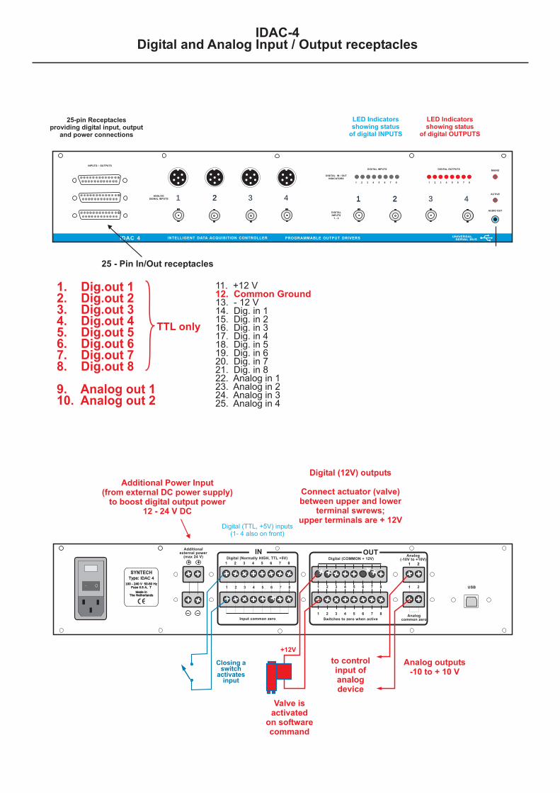
25-pin Receptaclesproviding digital input, output
and power connections
Additional Power Input(from external DC power supply)
to boost digital output power12 - 24 V DC
25 - Pin In/Out receptacles
Digital (TTL, +5V) inputs(1- 4 also on front)
Digital (12V) outputs
Connect actuator (valve)between upper and lower
terminal swrews;upper terminals are + 12V
Analog outputs-10 to + 10 V
IDAC-4Digital and Analog Input / Output receptacles
Closing aswitch
activatesinput
+12V
Valve isactivated
on softwarecommand
to controlinput ofanalogdevice
LED Indicatorsshowing status
of digital OUTPUTS
TTL only
11. +12 V
13. - 12 V14. Dig. in 115. Dig. in 216. Dig. in 317. Dig. in 418. Dig. in 519. Dig. in 620. Dig. in 721. Dig. in 822. Analog in 123. Analog in 224. Analog in 325. Analog in 4
12. Common Ground1. Dig.out 12. Dig.out 23. Dig.out 34. Dig.out 45. Dig.out 56. Dig.out 67. Dig.out 78. Dig.out 8
9. Analog out 110. Analog out 2
LED Indicatorsshowing status
of digital INPUTS
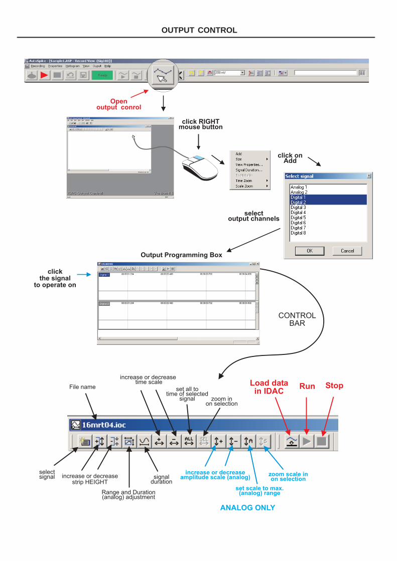
OUTPUT CONTROL
click onAdd
click RIGHTmouse button
selectoutput channels
clickthe signal
to operate on
CONTROLBAR
selectsignal signal
duration
increase or decreasetime scale
File name
zoom inon selection
set all totime of selected
signal
increase or decreaseamplitude scale (analog)
set scale to max.(analog) range
zoom scale inon selection
ANALOG ONLY
Load datain IDAC
Run Stop
increase or decreasestrip HEIGHT
Range and Duration(analog) adjustment
Output Programming Box
Openoutput conrol

19 OUTPUT CONTROL GENERAL IDAC-16 and IDAC-4
The Syntech signal acquisition systems IDAC-16 and IDAC-4 are provided with 8 digital and 2 analog programmable outputs. The digital outputs of the IDAC-16 are TTL (+5 V command signals) outputs only. Those of the IDAC-4 are configured both as TTL signals and as 12 - 24 V outputs capable of driving external actuators, like solenoid valves, without the need for interface electronics. A total power of 800 mA at 12 V can be delivered to the actuators. To drive devices at a higher total power rating or higher voltage (max. 24V) an external power supply can be connected. Programming
The on/off (0 / +5 V) status of the digital outputs and the voltage value (between -10 and +10 V) of the analog outputs is programmed using the IDAC OUTPUT CONTROL software, which is part of the Autospike program. The output states can be set with a temporal resolution of max.1 ms, and the analog values have an accuracy of 12 bit over the 20 V range. The maximum programmable time span is 10 hours. Trigger and time base
The programmed output sequence is triggered independently or linked to the signal acquisition of Autospike. Programmed TTL output signals can be used to (repeatedly) trigger acquisition and A/B control in Autospike, thus allowing time programming of consecutive Autospike recordings. Monitoring
The status of the digital outputs is monitored by the 8 LEDs on the front panel of the IDAC-4. Recording the status in Autospike of one or more digital input channels is possible by connecting the output signal(s) to the inputs. A ' loop back' connector for one of the 3 in/out 25-pin receptacles is available to wire all (TTL) outputs directly to the digital inputs. Analog signals
The analog outputs provide 'control signals' only, as they can only supply a max. current of 20 mA each. Most electronic mass flow controllers are provided with inputs directly compatible with this signal. To control the intensity of lights, or the direction and speed of motors, a suitable interface circuit is necessary. Consult Syntech for specific information about these applications.
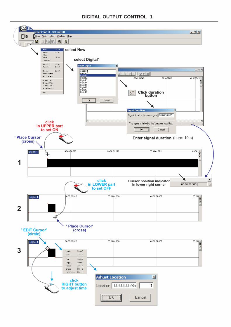
DIGITAL OUTPUT CONTROL 1
select New
select Digital1
clickin UPPER part
to set ON
clickin LOWER part
to set OFF
' Place Cursor'(cross)' EDIT Cursor'
(circle)
' Place Cursor'(cross)
clickRIGHT buttonto adjust time
1
2
3
Click durationbutton
Cursor position indicatorin lower right corner
Enter signal duration (here: 10 s)

20 PROGRAMMING DIGITAL OUTPUTS 1. Start IDAC Output Control The output control program is accessible in two ways: * After opening a project in Autospike: in the File menu: " Idac output control..."
* In the Wave recording mode: click the IO Control button. A new file can be created or an existing one opened in the File menu. 2. Open the 'Select signal' box to select the channels to be programmed. * By a RIGTH mouse click in the empty Control box, followed by 'add signal'. Or by a click on * In the ' Strip' menu select ' Add'. * Select the channels in the 'Select signal' box 3. Define the signal duration * Click the ' duration' button: * Enter the maximum duration of the programmed output sequence. 4. Adjust the height of the signal strips * Click the ' increase' or 'decrease' buttons: 5. Adjust the visible part of the total duration (zoom) * Click the " increase or 'decrease' buttons: 6. Select one of the signals to be programmed by a click on the name (Digital1,...8) 7. Setting 'ON' and ' OFF' points: * ON: place the cursor in the UPPER part of the strip and click LEFT. * OFF: place the cursor in the LOWER part of the strip and click LEFT. The exact position of the cursor is presented in the lower right corner of the box 8. Moving points: * Place the cursor on the point, keep the LEFT mouse button down while dragging the point 9. Editing points: * Place the cursor on the point. * The point turns GREEN after a LEFT mouse click * Click the RIGHT mouse button to open the edit menu. * Select ' Location..' to edit the exact location of the point
DIGITAL OUTPUT CONTROL 2
keep RIGHT buttondown to move ON point
keep LEFT buttondown to move OFF point
LEFT button downselect by dragging over
select ON point;to move selection
keep LEFT button down
click RIGHT buttonfor pop-up menu
click LEFT buttonfor position to paste
MOVEpoints
MOVEselection
COPYselection
SELECT

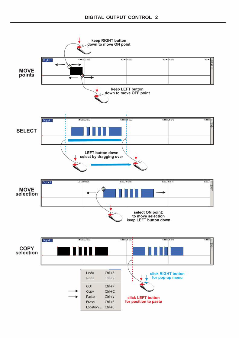
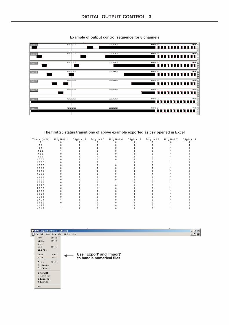
21 10. Select a sequence * Drag the mouse pointer with the LEFT button down over the section to be selected: The selected section turns into BLUE. 11. Move a selection * Place the cursor on any of the point in a selected section * Drag the section while keeping the LEFT mouse button down 12. Edit a selection * Place the cursor on any point in the selection * Click RIGHT for the edit menu to pop up. 13. Copy, and Paste * Select a section * Click RIGHT * Click ' Copy' * Place the cursor at the location to paste the selection (in the same signal or in any of the other signal strips) * Click RIGHT * Click ' Paste' 14. Save and Export * Program sequences can be saved as * ioc files, or * Exported as *csv (comma separated values), which can be opened and edited in Excel. 15. Editing and creating numerical output control files. * Open an exported file in Excel and edit the stored values * Create a new Excel file containing the required status times and changes of the output signals. * Only change times and values. Maintain the file format. * Import the new Excel file in the IOControl program. 16. Numerical file format * Time column: the time (in ms) of all status changes in any of the 8 signals is presented. In between consecutive times no status change occurs. * In the digital signal columns a ' 0' stands for OFF, and a '1' for ON. 17. Activating and running the output control sequence * Save the file or open an existing file. * Click the 'send data to IDAC' button: * Start the output: Click on * Stop: Click on
DIGITAL OUTPUT CONTROL 3
T i m e [ m S ] D i g i t a l 1 D i g i t a l 2 D i g i t a l 3 D i g i t a l 4 D i g i t a l 5 D i g i t a l 6 D i g i t a l 7 D i g i t a l 8
0 0 0 0 0 0 0 0 0
5 1 0 0 0 0 0 0 1 0
6 1 0 0 0 0 0 0 1 1
1 0 0 1 0 0 0 0 0 1 1
4 0 0 0 1 0 0 0 0 1 1
7 0 0 0 0 1 0 0 0 1 1
1 0 0 0 0 0 0 0 0 0 1 1
1 0 0 5 0 0 0 1 0 0 1 1
1 3 0 5 0 0 0 0 0 0 1 1
1 3 1 0 0 0 0 0 1 0 1 1
1 6 1 0 0 0 0 0 0 0 1 1
1 7 0 0 0 0 0 0 0 1 1 1
2 0 0 0 0 0 0 0 1 0 1 1
2 3 0 0 0 0 0 0 0 0 1 1
2 3 2 5 0 0 0 1 0 0 1 1
2 6 2 5 0 0 0 0 0 0 1 1
2 6 5 0 0 0 1 0 0 0 1 1
2 9 5 0 0 0 0 0 0 0 1 1
3 0 2 5 0 1 0 0 0 0 1 1
3 3 5 5 0 0 0 0 0 0 1 1
3 4 2 1 1 0 0 0 0 0 1 1
3 7 9 2 0 0 0 0 0 0 1 1
4 1 6 2 1 0 0 0 0 0 1 1
4 5 1 8 1 1 0 0 0 0 1 1
Example of output control sequence for 8 channels
Use ' Export' and 'Import'to handle numerical files
The first 25 status transitions of above example exported as csv opened in Excel
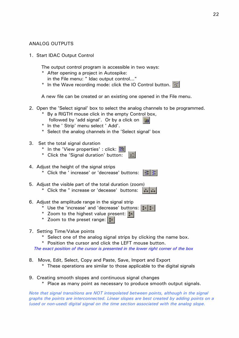
22 ANALOG OUTPUTS 1. Start IDAC Output Control The output control program is accessible in two ways: * After opening a project in Autospike: in the File menu: " Idac output control..."
* In the Wave recording mode: click the IO Control button. A new file can be created or an existing one opened in the File menu. 2. Open the 'Select signal' box to select the analog channels to be programmed. * By a RIGTH mouse click in the empty Control box, followed by 'add signal'. Or by a click on * In the ' Strip' menu select ' Add'. * Select the analog channels in the 'Select signal' box 3. Set the total signal duration * In the 'View properties' : click: * Click the 'Signal duration' button: 4. Adjust the height of the signal strips * Click the ' increase' or 'decrease' buttons: 5. Adjust the visible part of the total duration (zoom) * Click the " increase or 'decease' buttons: 6. Adjust the amplitude range in the signal strip * Use the 'increase' and 'decrease' buttons: * Zoom to the highest value present: * Zoom to the preset range: 7. Setting Time/Value points * Select one of the analog signal strips by clicking the name box. * Position the cursor and click the LEFT mouse button. The exact position of the cursor is presented in the lower right corner of the box 8. Move, Edit, Select, Copy and Paste, Save, Import and Export * These operations are similar to those applicable to the digital signals 9. Creating smooth slopes and continuous signal changes * Place as many point as necessary to produce smooth output signals.
Note that signal transitions are NOT interpolated between points, although in the signal graphs the points are interconnected. Linear slopes are best created by adding points on a (used or non-used) digital signal on the time section associated with the analog slope.
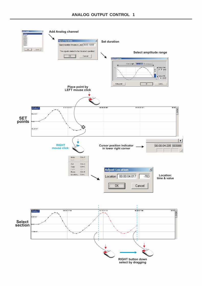
ANALOG OUTPUT CONTROL 1
Add Analog channel
Set duration
Select amplitude range
Place point byLEFT mouse click
Cursor position indicatorin lower right corner
Location:time & value
RIGHTmouse click:
RIGHT button downselect by dragging
SETpoints
Selectsection
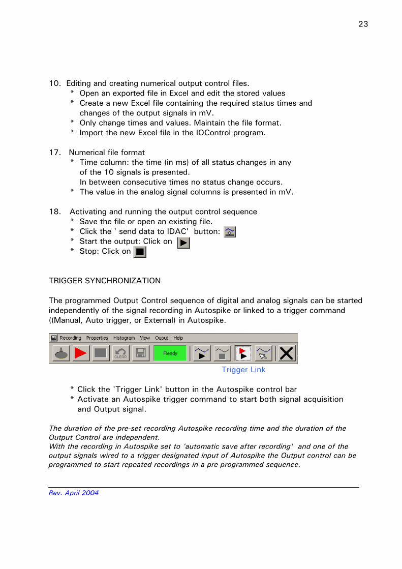
23 10. Editing and creating numerical output control files. * Open an exported file in Excel and edit the stored values * Create a new Excel file containing the required status times and changes of the output signals in mV. * Only change times and values. Maintain the file format. * Import the new Excel file in the IOControl program. 17. Numerical file format * Time column: the time (in ms) of all status changes in any of the 10 signals is presented. In between consecutive times no status change occurs. * The value in the analog signal columns is presented in mV. 18. Activating and running the output control sequence * Save the file or open an existing file. * Click the ' send data to IDAC' button: * Start the output: Click on * Stop: Click on TRIGGER SYNCHRONIZATION The programmed Output Control sequence of digital and analog signals can be started independently of the signal recording in Autospike or linked to a trigger command ((Manual, Auto trigger, or External) in Autospike.
Trigger Link * Click the 'Trigger Link' button in the Autospike control bar * Activate an Autospike trigger command to start both signal acquisition and Output signal. The duration of the pre-set recording Autospike recording time and the duration of the Output Control are independent. With the recording in Autospike set to 'automatic save after recording' and one of the output signals wired to a trigger designated input of Autospike the Output control can be programmed to start repeated recordings in a pre-programmed sequence. Rev. April 2004
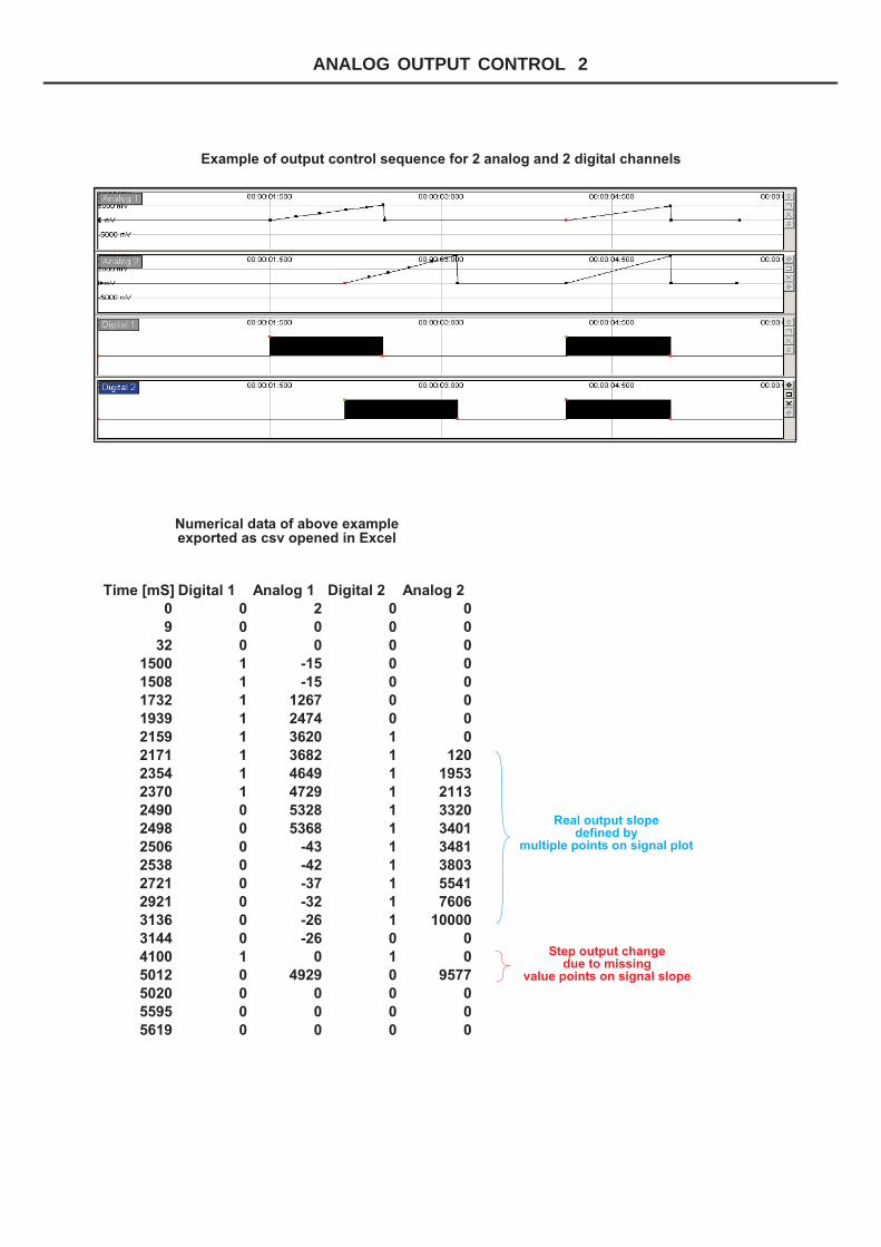
ANALOG OUTPUT CONTROL 2
Example of output control sequence for 2 analog and 2 digital channels
Numerical data of above exampleexported as csv opened in Excel
Time [mS] Digital 1 Analog 1 Digital 2 Analog 2
0 0 2 0 0
9 0 0 0 0
32 0 0 0 0
1500 1 -15 0 0
1508 1 -15 0 0
1732 1 1267 0 0
1939 1 2474 0 0
2159 1 3620 1 0
2171 1 3682 1 120
2354 1 4649 1 1953
2370 1 4729 1 2113
2490 0 5328 1 3320
2498 0 5368 1 3401
2506 0 -43 1 3481
2538 0 -42 1 3803
2721 0 -37 1 5541
2921 0 -32 1 7606
3136 0 -26 1 10000
3144 0 -26 0 0
4100 1 0 1 0
5012 0 4929 0 9577
5020 0 0 0 0
5595 0 0 0 0
5619 0 0 0 0
Real output slopedefined by
multiple points on signal plot
Step output changedue to missing
value points on signal slope
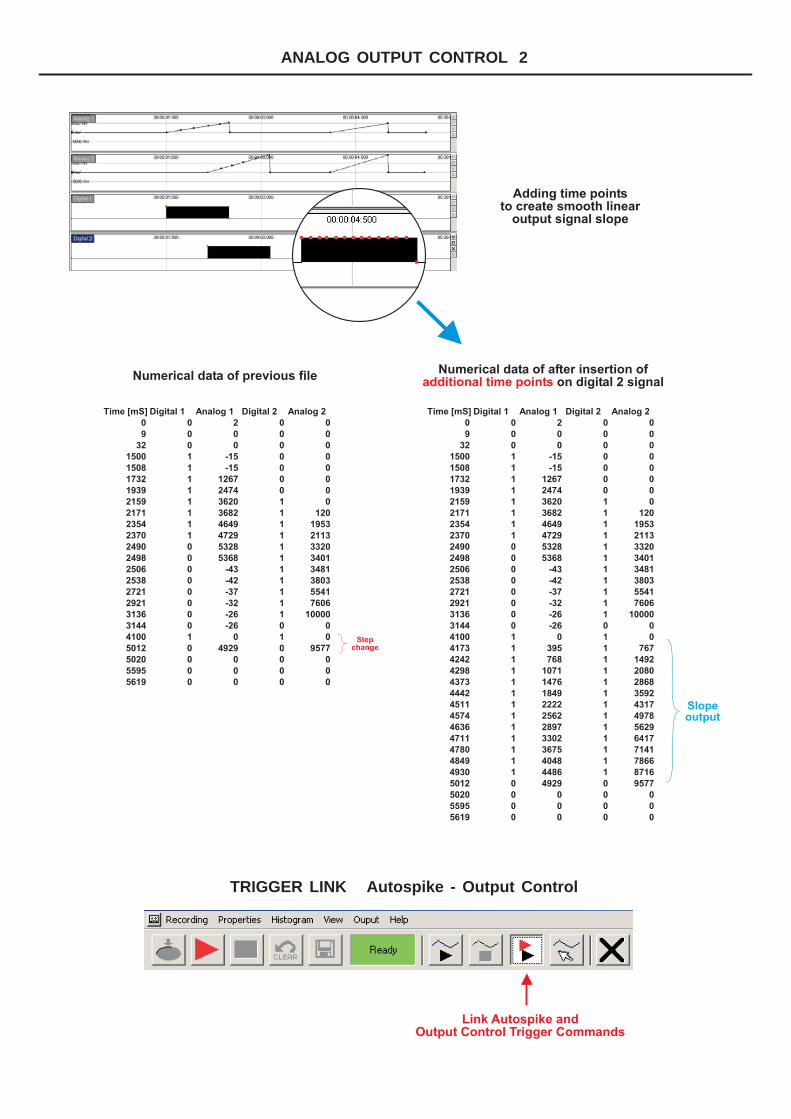
ANALOG OUTPUT CONTROL 2
TRIGGER LINK Autospike - Output Control
Time [mS] Digital 1 Analog 1 Digital 2 Analog 2
0 0 2 0 0
9 0 0 0 0
32 0 0 0 0
1500 1 -15 0 0
1508 1 -15 0 0
1732 1 1267 0 0
1939 1 2474 0 0
2159 1 3620 1 0
2171 1 3682 1 120
2354 1 4649 1 1953
2370 1 4729 1 2113
2490 0 5328 1 3320
2498 0 5368 1 3401
2506 0 -43 1 3481
2538 0 -42 1 3803
2721 0 -37 1 5541
2921 0 -32 1 7606
3136 0 -26 1 10000
3144 0 -26 0 0
4100 1 0 1 0
4173 1 395 1 767
4242 1 768 1 1492
4298 1 1071 1 2080
4373 1 1476 1 2868
4442 1 1849 1 3592
4511 1 2222 1 4317
4574 1 2562 1 4978
4636 1 2897 1 5629
4711 1 3302 1 6417
4780 1 3675 1 7141
4849 1 4048 1 7866
4930 1 4486 1 8716
5012 0 4929 0 9577
5020 0 0 0 0
5595 0 0 0 0
5619 0 0 0 0
Time [mS] Digital 1 Analog 1 Digital 2 Analog 2
0 0 2 0 0
9 0 0 0 0
32 0 0 0 0
1500 1 -15 0 0
1508 1 -15 0 0
1732 1 1267 0 0
1939 1 2474 0 0
2159 1 3620 1 0
2171 1 3682 1 120
2354 1 4649 1 1953
2370 1 4729 1 2113
2490 0 5328 1 3320
2498 0 5368 1 3401
2506 0 -43 1 3481
2538 0 -42 1 3803
2721 0 -37 1 5541
2921 0 -32 1 7606
3136 0 -26 1 10000
3144 0 -26 0 0
4100 1 0 1 0
5012 0 4929 0 9577
5020 0 0 0 0
5595 0 0 0 0
5619 0 0 0 0
Stepchange
Slopeoutput
Numerical data of previous file
Adding time pointsto create smooth linear
output signal slope
Link Autospike andOutput Control Trigger Commands
Numerical data of after insertion ofon digital 2 signaladditional time points