ieee 802.11b ad hoc networks: performance...
TRANSCRIPT

- 1 -
IEEE 802.11b Ad Hoc Networks: Performance Measurements
Giuseppe Anastasi
Dept. of Information Engineering, University of Pisa Via Diotisalvi 2 - 56122 Pisa, Italy
Email: [email protected]
Eleonora Borgia, Marco Conti, Enrico Gregori
Istituto IIT, National Research Council (CNR) Via G. Moruzzi - 1 56124 Pisa, Italy
Email: {eleonora.borgia, marco.conti, enrico.gregori}@iit.cnr.it Abstract. In this paper we investigate the performance of IEEE 802.11b ad hoc networks by means of an experimental study. An extensive literature, based on simulation studies, there exists on the performance of IEEE 802.11 ad hoc networks. Our analysis reveals several aspects that are usually neglected in previous simulation studies. Firstly, since different transmission rates are used for control and data frames, different transmission ranges and carrier-sensing ranges may exist at the same time in the network. In addition, the transmission ranges are in practice much shorter than usually assumed in simulation analysis, not constant but highly variable (even in the same session) and depends on several factors. Finally, the results presented in this paper indicate that for correctly understanding the behavior of an 802.11b network operating in ad hoc mode, several different ranges must be considered. In addition to the transmission range, the physical carrier sensing range is very important. The transmission range is highly dependent on the data rate and is up to 100 m, while the physical carrier sensing range is almost independent from the data rate and is approximately 200 m. Furthermore, even though stations are outside from their respective physical carrier sensing range, they may still interfere if their distance is lower than 350 m.
1 Introduction
The IEEE 802.11 technology [IEE02] is a good platform to implement single-hop ad hoc networks
because of its extreme simplicity. Single-hop means that stations must be within the same
transmission radium (say 100-200 meters) to be able to communicate. This limitation can be
overcome by multi-hop ad hoc networking. This requires the addition of routing mechanisms at
stations so that they can forward packets towards the intended destination, thus extending the range
of the ad hoc network beyond the transmission radium of the source station. Routing solutions
designed for wired networks (e.g., the Internet) are not suitable for the ad hoc environment,
primarily due to the dynamic topology of ad hoc networks. Even though large-scale multi-hop ad
hoc networks will not be available in the near future, on smaller scales, mobile ad hoc networks are
starting to appear thus extending the range of the IEEE 802.11 technology over multiple radio hops.

- 2 -
Most of the existing IEEE 802.11-based ad hoc networks have been developed in the academic
environment, but recently even commercial solutions have been proposed (see, e.g.,
MeshNetworks1 and SPANworks2).
The characteristics of the wireless medium and the dynamic nature of ad hoc networks make (IEEE
802.11) multi-hop networks fundamentally different from wired networks. Furthermore, the
behavior of an ad hoc network that relies upon a carrier-sensing random access protocol, such as the
IEEE 802.11, is further complicated by the presence of hidden stations, exposed stations,
“capturing” phenomena [XuS01, XuS02], and so on. The interactions between all these phenomena
make the behavior of IEEE 802.11 ad hoc networks very complex to predict. Recently, this has
generated an extensive literature related to the performance analysis of the 802.11 MAC protocol in
the ad hoc environment. Most of these studies have been done through simulation (to the best of our
knowledge, only very few experimental analysis have been conducted). Furthermore, they are based
on the original IEEE 802.11 standard operating at a maximum rate of 2 Mbps. Currently, however,
the IEEE 802.11b version, also known as Wi-Fi, is the reference technology for ad hoc networking.
For this reason, in this paper we extend the previous studies on IEEE 802.11 performance with an
extensive set of measurements conducted on a real testbed based on IEEE 802.11b products. The
measurements were done in an outdoor environment, by considering different traffic types (i.e.,
TCP and UDP traffics). Our experimental results indicate that transmission ranges are much shorter
than assumed in previous simulation studies. In addition, we also observed a dependency of
transmission range on the transmission speed. Finally, we found that even when two sessions are
outside from their respective physical carrier sensing range they may still interfere.
1 http://www.meshnetworks.com
2 http://www.spanworks.com

- 3 -
The paper is organized as follows. Section 2 gives an overview of the IEEE 802.11 architecture and
protocols. Section 3 describes the main problems of IEEE 802.11 ad hoc network and summarized
the main results obtained in previous (simulation) studies. The experimental analysis of the 802.11b
in ad hoc mode is presented in Section 4. Conclusions are drawn in Section 5.
2 IEEE 802.11 Architecture and Protocols
In this section we present the IEEE 802.11 architecture and protocols as defined in the original
standard [IEE99], with a particular attention to the MAC layer. Later, in Section 4, we will
emphasize the differences between the 802.11b standard with respect to the original 802.11
standard.
The IEEE 802.11 standard specifies both the MAC layer and the Physical Layer (see Figure 1). The
MAC layer offers two different types of service: a contention free service provided by the
Distributed Coordination Function (DCF), and a contention-free service implemented by the Point
Coordination Function (PCF). These service types are made available on top of a variety of
physical layers. Specifically, three different technologies have been specified in the standard:
Infrared (IF), Frequency Hopping Spread Spectrum (FHSS) and Direct Sequence Spread Spectrum
(DSSS).
The DCF provides the basic access method of the 802.11 MAC protocol and is based on a Carrier
Sense Multiple Access with Collision Avoidance (CSMA/CA) scheme. The PCF is implemented on
top of the DCF and is based on a polling scheme. It uses a Point Coordinator that cyclically polls
stations, giving them the opportunity to transmit. Since the PCF can not be adopted in ad hoc mode,
it will not be considered hereafter.

- 4 -
Physical Layer
contention freeservices contention
services
Distributed CoordinationFunction
Point CoordinationFunction
Figure 1. IEEE 802.11 Architecture.
According to the DCF, before transmitting a data frame, a station must sense the channel to
determine whether any other station is transmitting. If the medium is found to be idle for an interval
longer than the Distributed InterFrame Space (DIFS), the station continues with its transmission3
(see Figure 2). On the other hand (i.e., if the medium is busy), the transmission is deferred until the
end of the ongoing transmission. A random interval, henceforth referred to as the backoff time, is
then selected, which is used to initialize the backoff timer. The backoff timer is decreased for as
long as the channel is sensed as idle, stopped when a transmission is detected on the channel, and
reactivated when the channel is sensed as idle again for more than a DIFS (for example, the backoff
timer of Station 2 in Figure 2 is disabled while Station 3 is transmitting its frame; the timer is
reactivated a DIFS after Station 3 has completed its transmission). The station is enabled to transmit
its frame when the backoff timer reaches zero. The backoff time is slotted. Specifically, the backoff
time is an integer number of slots uniformly chosen in the interval (0, CW-1). CW is defined as the
Backoff Window, also referred to as Contention Window. At the first transmission attempt
CW=CWmin, and it is doubled at each retransmission up to CWmax. In the standard CWmin and
CWmax values depend on the physical layer adopted. For example, for the FHSS Phisical Layer
Cwmin and Cwmax values are 16 and 1024, respectively [IEE99].
3 To guarantee fair access to the shared medium, a station that has just transmitted a frame and has another frame ready
for transmission must perform the backoff procedure before initiating the second transmission.

- 5 -
Obviously, it may happen that two or more stations start transmitting simultaneously and a collision
occurs. In the CSMA/CA scheme, stations are not able to detect a collision by hearing their own
transmission (as in the CSMA/CD protocol used in wired LANs). Therefore, an immediate positive
acknowledgement scheme is employed to ascertain the successful reception of a frame.
Specifically, upon reception of a data frame, the destination station initiates the transmission of an
acknowledgement frame (ACK) after a time interval called Short InterFrame Space (SIFS). The
SIFS is shorter than the DIFS (see Figure 3) in order to give priority to the receiving station over
other possible stations waiting for transmission. If the ACK is not received by the source station,
the data frame is presumed to have been lost, and a retransmission is scheduled. The ACK is not
transmitted if the received frame is corrupted. A Cyclic Redundancy Check (CRC) algorithm is
used for error detection.
Station 1
Station 2
Station 3
FRAME
DIFS
FRAME
FRAME
DIFS DIFS
Packet Arrival
Frame Transmission
Elapsed Backoff Time
Residual Backoff Time
Figure 2. Basic Access Mechanism.
After an erroneous frame is detected (due to collisions or transmission errors), a station must remain
idle for at least an Extended InterFrame Space (EIFS) interval before it reactivates the backoff
algorithm. Specifically, the EIFS shall be used by the DCF whenever the physical layer has
indicated to the MAC that a frame transmission was begun that did not result in the correct
reception of a complete MAC frame with a correct FCS value. Reception of an error-free frame
during the EIFS re-synchronizes the station to the actual busy/idle state of the medium, so the EIFS
is terminated and normal medium access (using DIFS and, if necessary, backoff) continues
following reception of that frame.

- 6 -
Source Station
Destination Station
FRAME
DIFS SIFS
ACK
Packet Arrival
Figure 3. Interaction between the source and destination stations. The SIFS is shorter than the DIFS.
3 Common Problems in Wireless Ad Hoc Networks
In this section we shortly discuss the main problems that arise in wireless ad hoc networks. A
detailed discussion can be found in [Ana03]. The characteristics of the wireless medium make
wireless networks fundamentally different from wired networks. Specifically, as indicated in
[IEE99]:
- the wireless medium has neither absolute nor readily observable boundaries outside of
which stations are known to be unable to receive network frames;
- the channel is unprotected from outside signals;
- the wireless medium is significantly less reliable than wired media;
- the channel has time-varying and asymmetric propagation properties.
A B C
Figure 4. The “hidden station” problem.
In wireless (ad hoc) networks that rely upon a carrier-sensing random access protocol, like the IEEE
802.11, the wireless medium characteristics generate complex phenomena such as the hidden

- 7 -
station and the exposed station problems. Figure 4 shows a typical “hidden station” scenario. Let us
assume that station B is in the transmitting range of both A and C, but A and C can not hear each
other. Let us also assume that A is transmitting to B. If C has a frame to be transmitted to B,
according to the DFC protocol, it senses the medium and finds it free because it is not able to hear
A’s transmissions. Therefore, it starts transmitting the frame but this transmission will results in a
collision at the destination Station B.
Source Station
Destin. Station
Another Station
FRAME
DIFS
SIFS
DIFS
SIFS
SIFS
ACK
RTS
CTS
Backoff TimeNAV RTS
NAV CTS
Figure 5. Virtual Career Sensing mechanism.
The hidden station problem can be alleviated by extending the basic mechanism by a virtual
carrier sensing mechanism (also referred to as floor acquisition mechanism) that is based on two
control frames: Request To Send (RTS) and Clear To Send (CTS), respectively. According to this
mechanism, before transmitting a data frame, the source station sends a short control frame, named
RTS, to the receiving station announcing the upcoming frame transmission (see Figure 5). Upon
receiving the RTS frame, the destination station replies by a CTS frame to indicate that it is ready to
receive the data frame. Both the RTS and CTS frames contain the total duration of the transmission,
i.e., the overall time interval needed to transmit the data frame and the related ACK. This
information can be read by any station within the transmission range of either the source or the
destination station. Such a station uses this information to set up a timer called Network Allocation
Vector (NAV). While the NAV timer is greater than zero the station must refrain from accessing the
wireless medium. By using the RTS/CTS mechanism, stations may become aware of transmissions
from hidden station and on how long the channel will be used for these transmissions.
- 8 -
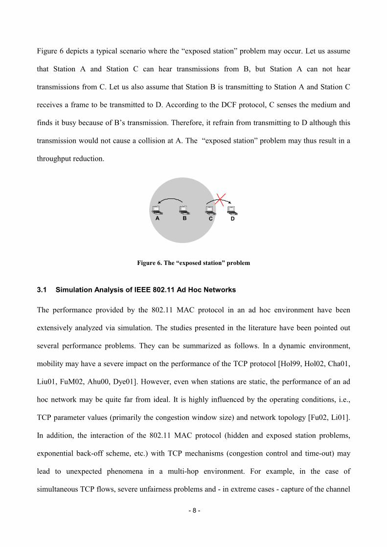
Figure 6 depicts a typical scenario where the “exposed station” problem may occur. Let us assume
that Station A and Station C can hear transmissions from B, but Station A can not hear
transmissions from C. Let us also assume that Station B is transmitting to Station A and Station C
receives a frame to be transmitted to D. According to the DCF protocol, C senses the medium and
finds it busy because of B’s transmission. Therefore, it refrain from transmitting to D although this
transmission would not cause a collision at A. The “exposed station” problem may thus result in a
throughput reduction.
A B C D
Figure 6. The “exposed station” problem
3.1 Simulation Analysis of IEEE 802.11 Ad Hoc Networks
The performance provided by the 802.11 MAC protocol in an ad hoc environment have been
extensively analyzed via simulation. The studies presented in the literature have been pointed out
several performance problems. They can be summarized as follows. In a dynamic environment,
mobility may have a severe impact on the performance of the TCP protocol [Hol99, Hol02, Cha01,
Liu01, FuM02, Ahu00, Dye01]. However, even when stations are static, the performance of an ad
hoc network may be quite far from ideal. It is highly influenced by the operating conditions, i.e.,
TCP parameter values (primarily the congestion window size) and network topology [Fu02, Li01].
In addition, the interaction of the 802.11 MAC protocol (hidden and exposed station problems,
exponential back-off scheme, etc.) with TCP mechanisms (congestion control and time-out) may
lead to unexpected phenomena in a multi-hop environment. For example, in the case of
simultaneous TCP flows, severe unfairness problems and - in extreme cases - capture of the channel

- 9 -
by few flows [Tan99, XuS01, XuS02, XuB02] may occur. Even in the case of a single TCP
connection, the instantaneous throughput may be very unstable [XuS01, XuS02]. Such phenomena
do not appear, or appear with less intensity, when the UDP protocol is used.
All these previous analysis were carried out using simulation tools (GloMosim [Glo02], ns-2
[Ns02], Qualnet [Qua02], etc.), and thus the results observed are highly dependent on the physical
layer model implemented in the simulation tool. In addition, these results have been obtained by
assuming the IEEE 802.11 original standard operating at 2 Mbps. Currently, however, the IEEE
802.11b is the de facto reference technology for ad hoc networking. Therefore, in our experimental
analysis, we investigate the performance of the IEEE 802.11b when operating in ad hoc mode. Our
results point out that several important aspects of IEEE 802.11b are not considered in the previous
studies.
4 Experimental Analysis of IEEE 802.11b Ad Hoc Networks
The 802.11b standard extends the 802.11 standard by introducing a higher-speed Physical Layer in
the 2.4 GHz frequency band still guaranteeing the interoperability with 802.11 cards. Specifically,
802.11b enables transmissions at 5.5 Mbps and 11 Mbps, in addition to 1 Mbps and 2 Mbps.
802.11b cards may implement a dynamic rate switching with the objective of improving
performance. To ensure coexistence and interoperability among multirate-capable stations, and with
802.11 cards, the standard defines a set of rules that must be followed by all stations in a WLAN.
Specifically, for each WLAN is defined a basic rate set that contains the data transfer rates that all
stations within the WLAN will be capable of using to receive and transmit.
To support the proper operation of a WLAN, all stations must be able to detect control frames.
Hence, RTS, CTS, and ACK frames must be transmitted at a rate included in the basic rate set. In
addition, frames with multicast or broadcast destination addresses must be transmitted at a rate

- 10 -
belonging to the basic rate set. These differences in the rates used for transmitting (unicast) data and
control frames has a big impact on the system behavior as clearly pointed out in [Eph02].
Actually, since 802.11b cards transmit at a constant power, lowering the transmission rate permits
the packaging of more energy per symbol, and this makes the transmission range increasing. In the
next subsections we investigate, by a set of experimental measurements,
i) the relationship between the transmission rate of the wireless network interface card
(NIC) and the maximum throughput (two-stations experiments);
ii) the relationship between the transmission and carrier sensing range and the transmission
rate (two-stations experiments);
iii) Hidden and/or exposed station situations (four-stations experiments).
To better understand the results presented below, it is useful to provide a model of the relationships
existing among stations when they transmit or receive. In particular, it is useful to make a
distinction between the transmission range, the interference range and the carrier sensing range. The
following definitions can be given.
�� The Transmission Range (TX_range) is the range (with respect to the transmitting station)
within which a transmitted frame can be successfully received. The transmission range is
mainly determined by the transmission power and the radio propagation properties.
�� The Physical Carrier Sensing Range (PCS_range) is the range (with respect to the transmitting
station) within which the other stations detect a transmission. It mainly depends on the
sensitivity of the receiver (the receive threshold) and the radio propagation properties.
�� The Interference Range (IF_range) is the range within which stations in receive mode will be
"interfered with" by a transmitter, and thus suffer a loss. The interference range is usually
larger than the transmission range, and it is function of the distance between the sender and
receiver, and of the path loss model.

- 11 -
In the previous simulation studies the following relationship has been generally assumed:
rangePCSrangeIFrangeTX ___ �� . For example, in the ns-2 simulation tool [Ns02] the
following values are used to model the characteristics of the physical layer: TX _ range� 250m ,
IF _ range � PCS _ range � 550m . In addition, the relationship between rangeTX _ , rangePCS _ ,
and rangeIF _ are assumed to be constant throughout a simulation experiment. On the other hand,
from our measurements we have observed that the physical channel has time-varying and
asymmetric propagation properties and, hence, the value of rangeTX _ , rangePCS _ , and
rangeIF _ may be highly variable in practice.
4.1 Available Bandwidth
In this section we will show that only a fraction of the 11 Mbps nominal bandwidth of the IEEE
802.11b cards can be used for data transmission. To this end we need to carefully analyze the
overheads associated with the transmission of each packet (see Figure 7). Specifically, each stream
of m bytes generated by a legacy Internet application is encapsulated by the TCP/UDP and IP
protocols that add their headers before delivering the resulting IP datagram to the MAC layer for
transmission over the wireless medium. Each MAC data frame is made up of: i) a MAC header, say
MAChdr , containing MAC addresses and control information,4 and ii) a variable length data
payload, containing the upper layers data information. Finally, to support the physical procedures of
transmission (carrier sense and reception) a physical layer preamble (PLCP preamble) and a
physical layer header (PLCP header) have to be added to both data and control frames. Hereafter,
we will refer to the sum of PLCP preamble and PLCP header as PHYhdr .
4 Without any loss of generality we have considered the frame error sequence ( FCS), for error detection, as belonging
to the MAC header.

- 12 -
m Bytes
TCP/UDP payload
IP payload
Hdr
Hdr
MAC payloadHdr+FCS
PSDUPHY Hdr
TDATA
ApplicationLayer
TransportLayer
NetworkLayer
MACLayer
PhysicalLayer
Figure 7. Encapsulation overheads.
It is worth noting that these different headers and data fields are transmitted at different data rates to
ensure the interoperability between 802.11 and 802.11b cards. Specifically, the standard defines
two different formats for the PLCP: Long PLCP and Short PLCP. Hereafter, we assume a Long
PLCP that includes a 144-bit preamble and a 48-bit header both transmitted at 1 Mbps while the
MAChdr and the MACpayload can be transmitted at one of the NIC data rates: 1, 2, 5.5, and 11 Mbps.
In particular, control frames (RTS, CTS and ACK) can be transmitted at 1 or 2 Mbps, while data
frame can be transmitted at any of the NIC data rates.
By taking into considerations the above quantities Equation (1) defines the maximum expected
throughput for a single active session (i.e., only a sender-receiver couple active) when the basic
access scheme (i.e., DCF and no RTS-CTS) is used. Specifically, Equation (1) is the ratio between
the time required to transmit the user data and the overall time the channel is busy due to this
transmission:
TimeSlotCWTSIFSTDIFS
mThACKDATA
CTSnoRTS
_*2min/
����
� (1)
where
m is the number of bytes generated by the application.

- 13 -
TDATA is the time required to transmit a MAC data frame using one of the NIC data rate, i.e., 1, 2,
5.5 or 11 Mbps; this includes the PHYhdr , MAChdr , MACpayload and FCS bits for error detection.
TACK is the time required to transmit a MAC ACK frame; this includes the PHYhdr , and MAChdr .
CW min2
* Slot_Time is the average back off time.
When the RTS/CTS mechanism is used, the overheads associated with the transmission of the RTS
and CTS frames must be added to the denominator of (1). Hence, in this case, the maximum
throughput ThRTS /CTS , is defined as
TimeSlotCWSIFSTTTTDIFS
mThACKDATACTSRTS
CTSRTS
_*2min*3
/
������
� (2)
where TRTS and TCTS indicate the time required to transmit the RTS and CTS frames, respectively.
Equation (1) and (2) are used to obtain the theoretical throughput for a single session with UDP
traffic. Indeed, when using the TCP protocol, overheads due to the TCP_ACK transmission must be
considered. More precisely, the technique of cumulative ACK answering to two consecutive
TCP_DATA is used, so a TCP handshake is composed by TCP_DATA1, TCP_DATA2 and
TCP_ACK.
Figure 8 and Figure 9 show the TCP handshake on the channel when using the basic acess
mechanism and the RTS/CTS mechanism, respectively. In particular, DATA1 and DATA2 packets
are obtained by the encapsulation of TCP_DATA1 and TCP_DATA2, instead DATA3 is obtained
by the encapsulation of the TCP_ACK.

- 14 -
DIFS
DATA 1
Frame
ACK Destination
So urce
DIFS
SIFS ACK
DIFS
DATA 2
DATA 3
ACK
SIFS
SIFS CW
CW
CW
Y2Y1 Y3
Figure 8. TCP handshake with the basic mechanism.
SIFS
SIFS
DIFS
SIFS
SIFS
DATA 1 Frame
ACK Destination
Source
DIFS
CW
Y1
RTS
CTS
SIFS
SIFS ACK
DIFS
CW
SIFS
RTS
CTS
CW
DATA 2Frame
DATA 3Frame
RTS
SIFS
SIFS ACKCTS
Y2 Y3
Figure 9. TCP handshake with the RTS/CTS mechanism.
Thus, the theoretical throughput is the ratio between the time to transmit two user data frame and
the overall time for the complete transmission on the channel:
(3)
where yi represents the time required to the transmission of the DATAi packet on the channel.
The numerical results presented in the next sections depend on the specific setting of the IEEE
802.11b protocol parameters. Table 1 gives the values for the protocol parameters used hereafter.
321
2yyy
mTh��
��

- 15 -
Table 1. IEEE 802.11b parameter values.
Slot_ Time � PHYhdr MAChdr Bit Rate (Mbps)
20 µsec ≤1 µsec 192 bits (9.6 tslot) 272 bits 1, 2, 5.5, 11
DIFS SIFS ACK CWMIN CWMAX
50 µsec 10 µsec 112 bits + PHYhdr 32 tslot 1024 tslot
Table 2. Maximum throughputs in Mbit/sec (Mbps) at different data rates for a UDP connection.
m= 512 Bytes m=1024 Bytes
No RTS/CTS RTS/CTS No RTS/CTS RTS/CTS
11 Mbps 3.337 Mbps 2.739 Mbps 5.120 Mbps 4.386 Mbps
5,5 Mbps 2.490 Mbps 2.141 Mbps 3.428 Mbps 3.082 Mbps
2 Mbps 1.319 Mbps 1.214 Mbps 1.589 Mbps 1.511 Mbps
1 Mbps 0.758 Mbps 0.738 Mbps 0.862 Mbps 0.839 Mbps
Table 3. Maximum throughputs in Mbit/sec (Mbps) at different data rates for a TCP connection. n
m= 512 Bytes m=1024 Bytes
No RTS/CTS RTS/CTS No RTS/CTS RTS/CTS
11 Mbps 2.456 Mbps 1.979 Mbps 4.015 Mbps 3.354 Mbps
5,5 Mbps 1.931 Mbps 1.623 Mbps 2.858 Mbps 2.507 Mbps
2 Mbps 1.105 Mbps 0.997 Mbps 1.423 Mbps 1.330 Mbps
1 Mbps 0.661 Mbps 0.620 Mbps 0.796 Mbps 0.766 Mbps
In Table 2 and Table 3 we report the expected throughputs (with and without the RTS/CTS
mechanism), for different data rates, for a UDP and TCP connection, respectively. These results are

- 16 -
computed by applying Equations (1) and (2) and (3), and assuming a data packet size at the
application level equal to m=512 or m=1024 bytes.
As shown in the above tables, only a small percentage of the 11 Mbps nominal bandwidth can be
really used for data transmission. Obviously, this percentage increases with the payload size.
However, even with large packets sizes (e.g., m=1024 bytes) the bandwidth utilization is in the
order of 46% for UDP traffic and 36% for TCP traffic.
0
0.5
1
1.5
2
2.5
3
3.5
no RTS RTS/CTS
11 Mbps TCP
idealreal TCP
Thro
ughp
ut (M
bps)
0
0.5
1
1.5
2
2.5
3
3.5
no RTS RTS/CTS
11 Mbps UDP
idealreal UDP
Thro
ughp
ut (
Mbp
s)
Figure 10. Comparison between the theoretical maximum throughput and the actual throughput achieved by
TCP/UDP applications.
The above theoretical analysis has been complemented with measurements of the actual throughput
at the application level in a real environment. Specifically, we have considered two types of
applications: ftp and CBR. In the former case the TCP protocol is used at the transport layer, while
in the latter case the UDP is adopted. In both cases the applications operate in asymptotic
conditions (i.e., they always have packets ready for transmission) with constant size packets of 512
bytes. The results obtained from this experimental analysis are reported in Figure 10. The
experimental results related to the UDP traffic are very close to the maximum throughput computed
analytically. On the other hand, in the presence of the TCP protocol the measured throughput is
much lower than the theoretical maximum throughput, as expected. Similar results have been also

- 17 -
obtained by comparing the maximum throughput derived according to (1) and (2), and the real
throughputs measured when the NIC data rate is set to 1, 2 or 5.5 Mbps.
4.2 Transmission Ranges
The dependency between the data rate and the transmission range was investigated by measuring
the packet loss rate experienced by two communicating stations whose network interfaces transmit
at a constant (preset) data rate. Specifically, four sets of measurements were performed
corresponding to the different data rates: 1, 2, 5.5, and 11 Mbps. In each set of experiments the
packet loss rate was recorded as a function of the distance between the communicating stations. The
results are summarized in Table 4, where the estimates of the transmission ranges at different data
rates are reported. These estimates point out that, when using the highest bit rate for the data
transmission, there is a significant difference in the transmission range of control and data frames,
respectively. For example, assuming that the RTS/CTS mechanism is active, if a station transmits a
frame at 11 Mbps to another station within its transmission range (i.e., less then 30 m apart) it
reserves the channel for a radius of approximately 90 (120) m around itself. The RTS frame is
transmitted at 2 Mbps (or 1 Mbps), and hence, it is correctly received by all stations within station
transmitting range, i.e., 90 (120) meters.
Again, it is interesting to compare the transmission range used in the most popular simulation tools,
like ns-2 and Glomosim, with the transmission ranges measured in our experiments. In these
simulation tools it is assumed TX _ range� 250m . Since the above simulation tools only consider a
2-Mbps bit rate we make reference to the transmission range estimated with a NIC data rate of 2
Mbps. As it clearly appears, the value used in the simulation tools (and, hence, in the simulation
studies based on them) is 2-3 times higher that the values measured in practice. This difference is
very important for example when studying the behavior of routing protocols: the shorter is the
TX_range, the higher is the frequency of route re-calculation when the network stations are mobile.

- 18 -
Table 4. Estimates of the transmission ranges at different data rates.
11 Mbps 5.5 Mbps 2 Mbps 1 Mbps
Data TX_range 30 meters 70 meters 90-100 meters 110-130 meters
Control TX_range � 90 meters � 120 meters
4.3 Physical Carrier Sensing Range
The previous results show that the IEEE 802.11b behavior is more complex than the behavior of the
original IEEE 802.11 standard. Indeed the availability of different transmission rates may cause the
presence of several transmission ranges inside the network. In particular, inside the same data
transfer session there may be different transmission ranges for data and control frame (e.g., RTS,
CTS, ACK). Hereafter, we show that the superposition of these different phenomena makes very
difficult to understand the behavior of IEEE 802.11b ad hoc networks. To reduce this complexity,
in the experiments presented below the NIC data rate is set to a constant value for the entire
duration of the experiment.5
Two sets of experiments were performed by varying the NIC data rate. In the each set of
experiments the data rate is constant, and equal to 11 Mbps, and 2 Mbps, respectively. The same
four-stations configuration is considered in both cases but the distance between the two couples of
stations is different to take into account the different transmission range. The network
configurations are shown in Figure 11 and Figure 13, while the related results are presented in
Figure 12 and Figure 14, respectively. These results are the superposition of several factors that
5 It is worth pointing out that we experienced a high variability in the channel conditions thus making a comparison
between the results difficult.

- 19 -
make the system behavior similar in the two cases (even though numerical values differ due to the
different transmission rates).
Session 1 Session 2
25 m 80/85 m 25 m
S1 S2 S3 S4
Figure 11. Network configuration at 11 Mbps.
0
500
1000
1500
2000
2500
no RTS RTS/CTS
UDP
1->23->4
Thro
ughp
ut (
Kbps
)
0
500
1000
1500
2000
2500
no RTS RTS/CTS
TCP
1->23->4
Thro
ughp
ut (
Kbps
)
Figure 12. Throughputs at 11 Mbps.
In the first set of experiments (11Mbps) dependencies there exist between the two connections even
though the transmission range is smaller than the distance between stations S1 and S3. Furthermore,
the dependency exists also when the basic mechanism (i.e., no RTS/CTS) is adopted.6 To
summarize, this set of experiments show that i) interdependencies among the stations extends
beyond the transmission range; ii) our hypothesis is that the physical carrier sensing range,
including all the four stations, produces a correlation between active connections and its effect is
similar to that achieved with the RTS/CTS mechanism (virtual carrier sensing). The difference in
the throughputs achieved by the two sessions when using the UDP protocol (with or without
RTS/CTS) can be explained by considering the asymmetric condition that exists on the channel:
6 A similar behavior is observed (but with different values) by adopting the RTS/CTS mechanism.

- 20 -
station S2 is exposed to transmissions of station S3 and, hence, when station S1 sends a frame to S2
this station is not able to send back the MAC ACK. Therefore, S1 reacts as in the collision cases
(thus re-scheduling the transmission with a larger backoff). It is worth pointing out that also S3 is
exposed to S2 transmissions but the S2’s effect on S3 is less marked given the different role of the
two stations. When using the basic access mechanism, the S2’s effect on S3 is limited to short
intervals (i.e., the transmission of ACK frames). When adopting the RTS/CTS mechanism, the S2
CTS forces S3 to defer the transmission of RTS frames (i.e., simply a delay in the transmission),
while RTS frames sent by S3 forces S2 to not reply with a CTS frame to S1’s RTS. In the latter
case, S1 increases the back off and reschedules the transmission. Finally, when the TCP protocol is
used the differences between the throughput achieved by the two connections still exist but are
reduced. The analysis of this case is very complex because we must also take into consideration the
impact of the TCP mechanisms that: i) reduces the transmission rate of the first connection, and ii)
introduces the transmission of TCP-ACK frames (from S2 and S4) thus contributing to make the
system less asymmetric.
Session 1 Session 2
25 m 90/95 m 25 m
S1 S2 S3 S4
Figure 13. Network configuration at 2 Mbps.
In the second set of experiments (data rate equal to 2Mbps), whose results are presented in Figure
14, S2 and S3 are within the same transmission range and, in addition, it can assumed that all
stations are within the same physical carrier sensing range. It is also worth noting that in this case
the system is more balanced from the throughput standpoint. This can be expected as by
transmitting with a 2-Mbps data rate the transmission range is significantly larger than with the 11-
Mbps transmission rate, and hence the stations have a more uniform view of the channel status.

- 21 -
0
200
400
600
800
1000
1200
no RTS RTS/CTS
UDP
1->23->4
Thro
ughp
ut (
Kbps
)
0
200
400
600
800
1000
1200
no RTS RTS/CTS
TCP
1->23->4
Thro
ughp
ut (
Kbps
)
Figure 14. Throughputs at 2 Mbps.
We have performed several other experiments by considering the symmetric scenario shown in
Figure 15. The results obtained at 11 Mbps and 2 Mbps are reported in Figure 16 and Figure 17,
respectively. These results are aligned with the previous observations.
Session 1 Session 2
25 m 60/65 m 25 m
S1 S2 S3 S4
Figure 15. Simmetric Scenario.
0
500
1000
1500
2000
2500
3000
no RTS RTS/CTS
UDP
1->24->3
Thro
ughp
ut (
Kbps
)
0
500
1000
1500
2000
2500
3000
no RTS RTS/CTS
TCP
1->24->3
Thro
ughp
ut (
Kbps
)
Figure 16. Throughputs at 11 Mbps.
- 22 -
0
200
400
600
800
1000
1200
1400
no RTS RTS/CTS
UDP
1->24->3
Thro
ughp
ut (
Kbps
)
0
200
400
600
800
1000
1200
1400
no RTS RTS/CTS
TCP
1->24->3
Thro
ughp
ut (
Kbps
)
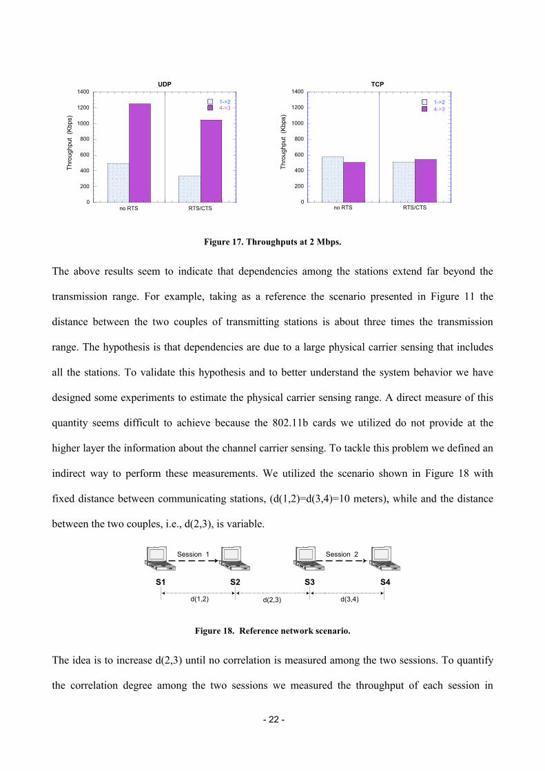
Figure 17. Throughputs at 2 Mbps.
The above results seem to indicate that dependencies among the stations extend far beyond the
transmission range. For example, taking as a reference the scenario presented in Figure 11 the
distance between the two couples of transmitting stations is about three times the transmission
range. The hypothesis is that dependencies are due to a large physical carrier sensing that includes
all the stations. To validate this hypothesis and to better understand the system behavior we have
designed some experiments to estimate the physical carrier sensing range. A direct measure of this
quantity seems difficult to achieve because the 802.11b cards we utilized do not provide at the
higher layer the information about the channel carrier sensing. To tackle this problem we defined an
indirect way to perform these measurements. We utilized the scenario shown in Figure 18 with
fixed distance between communicating stations, (d(1,2)=d(3,4)=10 meters), while and the distance
between the two couples, i.e., d(2,3), is variable.
Session 1 Session 2
d(1,2) d(2,3) d(3,4)
S1 S2 S3 S4
Figure 18. Reference network scenario.
The idea is to increase d(2,3) until no correlation is measured among the two sessions. To quantify
the correlation degree among the two sessions we measured the throughput of each session in

- 23 -
isolation, i.e., when the other session is not active. Then we measured the throughput achieved by
each session when both sessions are active. Obviously, no correlation exists when the aggregate
throughput is equal to the sum of the throughput of the two sessions in isolation. By varying the
distance d(2,3) we performed several experiments. The results were obtained with the cards
transmission rates set to 11 and 2 Mbps, and are summarized in Figure 19-left and Figure 19-right,
respectively. As it clearly appears from the figures, there are two steps in the aggregate throughput:
one after 180 m and the other after 250 m. This behavior can be explained as follows. Taken a
session as a reference, the presence of the other session may have two possible effects on the
performance of the reference session: 1) if the two sessions are within the same physical carrier
sensing range, they share the same physical channel; 2) if they are outside the physical carrier
sensing range the radiated energy from one session may still affect the quality of the channel
observed by the other session. As the radiated energy may travel over unlimited distances, we can
expect that the second effect completely disappears only for very large distances among the
sessions [Eph02]. Hence, we can assume that the first step coincides with the end of the physical
carrier sensing range, while the second one occurs even when the second effect becomes almost
negligible.
0
1000
2000
3000
4000
5000
6000
7000
100 150 200 250 300 350 400
11 Mbps
aggr
egat
e th
roug
hput
(Kbp
s)
distance between sessions (m)
independent sessions
0
500
1000
1500
2000
2500
3000
100 150 200 250 300 350 400
2 Mbps
aggr
egat
e th
roug
hput
(Kbp
s)
distance between sessions (m)
independent sessions
Figure 19. Aggregate Throughput vs. distance between sessions at 11 Mbps (left) and 2 Mbps (right). The
payload size is 512 byte in both cases.

- 24 -
It is worth noting that the physical carrier sensing range is almost the same for the two different
transmission rates. Indeed the physical carrier sensing mainly depends only on two parameters: the
stations’ transmitting power and the distance between transmitting stations. The rate at which data
are transmitted have no significant effect on these parameters.
The results obtained confirm the hypotheses we made above to justify the apparent dependencies
existing between the two couples of transmitting stations even if the distance among them is about
three times greater than the transmission range (see, for example, Figure 12 and Figure 14).
To summarize, the results presented in this paper indicate that, for correctly understanding the
behavior of an 802.11 network operating in ad hoc mode, several different ranges must be
considered. In addition to the transmission range, the physical carrier sensing range is very
important. Furthermore, even though stations are outside from their respective physical carrier
sensing range, they may still interfere.
5 Conclusions
In this paper we have investigated the performance of IEEE 802.11b ad hoc networks. Previous
studies in this framework have pointed out that the behavior of IEEE 802.11 ad hoc networks are
complicated by the presence of hidden stations, exposed stations, “capturing” phenomena, and so
on. Most of these studies have been done through simulation. In this paper we have extended the
802.11 performance analysis with an extensive set of measurements performed on a real testbed by
considering IEEE 802.11b cards. Our analysis has pointed out several aspects that are commonly
neglected in simulation studies. Specifically, the system behavior is very complex as several
transmission and carrier-sensing ranges there exist at the same time on the channel. For example,
the physical level preamble is always transmitted at 1Mbps, the signaling frames can be transmitted
up to 2 Mbps, while the data frames can be transmitted up to 11 Mbps. As a consequence of this
complex behavior, with IEEE 802.11b, we never observed capture phenomena (i.e., it never
- 25 -
happened that a couple of stations monopolized the channel). Finally, in simulation studies the
transmission and carrier sensing ranges are quite large, and constant for the entire duration of the
experiment. On the other hand, in our testbed we have observed that the transmission and physical
sensing ranges are much shorter than assumed in simulation studies, and highly variable even in the
same session in time and space, depending on several factors (whether condition, place and time of
the experiment, etc.).
Acknowledgements This work have been carried out partially under the financial support of MIUR (Italian Ministry for Education and Scientific Research) in the framework of the VICOM (Visual Immersive Communications) project and partially under the financial support of the European Union in the framework of the MobileMAN project. The authors wish to express their gratitude to Riccardo Bettarini for the help in performing the measurements presented in this paper.
References
[Ahu00] A. Ahuja et al., “Performance of TCP over different routing protocols in mobile ad-hoc networks,” Proceedings of IEEE Vehicular Technology Conference (VTC 2000), Tokyo, Japan, May 2000.
[Ana03] G. Anastasi, M. Conti, E. Gregori, “IEEE 802.11 Ad Hoc Networks: Protocols, Performance and Open Issues “, in Mobile Ad hoc networking, S. Basagni, M. Conti, S. Giordano, I. Stojmenovic (Editors), IEEE Press and John Wiley and Sons, Inc., New York, 2003.
[Cha01] K. Chandran, S. Raghunathan, S. Venkatesan, R. Prakash, “A Feedback Based Scheme for Improving TCP Performance in Ad Hoc Wireless Networks”, IEEE Personal Communication Magazine, Special Issue on Ad Hoc Networks, Vol. 8, N. 1, pp. 34-39, February 2001.
[Dye01] T.D. Dyer, R.V. Boppana “A Comparison of TCP Performance over Three Routing Protocols for Mobile Ad Hoc Networks”, Proc. ACM Symposium on Mobile Ad Hoc Networking & Computing (MobiHoc), October 2001.
[Eph02] T. Ephremides, “A Wireless Link Perspective in Mobile Networking", ACM Mobicom 2002 keynote speech, available at http://www.acm.org/sigmobile/mobicom/2002/program/
[Fu02] Z. Fu, P. Zerfos, K. Xu, H. Luo, S. Lu, L. Zhang, M. Gerla, “On TCP Performance in Multihop Wireless Networks“, UCLA Technical Report, 2002 (available at http://www.cs.ucla.edu/~hluo/publications/WINGTR0203.pdf) .
[FuM02] Z. Fu, X. Meng, S. Lu, “How Bad TCP Can Perform in Mobile Ad Hoc Networks”, Proceedings of the IEEE Symposium on Computers and Communications, Taormina-Giardini Naxos (Italy), July 2002, pp. 298-303.
[Glo02] GloMoSim, Global Mobile Information Systems Simulation Library, http://pcl.cs.ucla.edu/projects/glomosim/.
[Hol99] G. Holland, N. Vaidya, “Analysis of the TCP Performance over Mobile Ad Hoc Networks”, Proceedings of the ACM International Conference on Mobile Computing and Networking

- 26 -
(MobiCom’99), Seattle (WA), August 1999, pp. 207-218.
[Hol02] Gavin Holland, Nitin H. Vaidya “Analysis of TCP Performance over Mobile Ad Hoc Networks”, ACM/Kluwer Journal of Wireless Networks 8(2-3), (2002) pp. 275-288.
[IEE02] Official Homepage of the IEEE 802.11 Working Group, http://grouper.ieee.org/groups/802/11/.
[IEE99] IEEE standard 802.11, “Wireless LAN Medium Access Control (MAC) and Physical Layer (PHY) Specifications, August 1999.
[Li01] J. Li, C. Blake, D. De Couto, H. Lee, R. Morris, “Capacity of Wireless Ad Hoc Wireless Networks”, Proceedings of the ACM International Conference on Mobile Computing and Networking (MobiCom’01), Rome (I), July 2002, pp. 61-69.
[Liu01] J. Liu, S. Singh, “ATCP: TCP for mobile ad hoc networks”, IEEE Journal on Selected Areas in Communications, 19(7):1300-1315, July 2001.
[Ns02] The Network Simulator - ns-2, http://www.isi.edu/nsnam/ns/index.html.
[Qua02] Qualnet simulator, http://www.qualnet.com/.
[Tan99] K. Tang, M. Gerla, “Fair Sharing of MAC under TCP in Wireless Ad Hoc Networks”, Proceedings of IEEE MMT’99, Venice (I), October 1999.
[XuS01] S. Xu and T. Saadawi, “Does the IEEE 802.11 MAC protocol Work Well in Multihop Wireless Ad Hoc Networks?”, IEEE Communication Magazine, Volume 39, N. 6, June 2001, pp. 130-137.
[XuS02] S. Xu and T. Saadawi, “Revealing the Problems with 802.11 MAC Protocol in Multi-hop Wireless Networks”, Computer Networks, Volume 38, N. 4, March 2002.
[XuB02] K. Xu, S. Bae, S. Lee, M. Gerla, “TCP Behavior across Multihop Wireless Networks and the Wired Networks”, Proceedings of the ACM Workshop on Mobile Multimedia (WoWMoM 2002), Atlanta (GA), September 28, 2002, pp. 41-48.