ieee transaction on knowledge and data engineering, … · expressive numerical representation of...

IEEE TRANSACTION ON KNOWLEDGE AND DATA ENGINEERING, VOL. 16, NO. 8, AUGUST 2018 1

CURE: Flexible Categorical Data Representationby Hierarchical Coupling Learning

Songlei Jian, Guansong Pang, Longbing Cao, Senior Member, IEEE, Kai Lu , Hang Gao

Abstract—The representation of categorical data with hierarchical value coupling relationships (i.e., various value-to-value clusterinteractions) is very critical yet challenging for capturing complex data characteristics in learning tasks. This paper proposes a noveland flexible coupled unsupervised categorical data representation (CURE) framework, which not only captures the hierarchicalcouplings but is also flexible enough to be instantiated for contrastive learning tasks. CURE first learns the value clusters of differentgranularities based on multiple value coupling functions and then learns the value representation from the couplings between theobtained value clusters. With two complementary value coupling functions, CURE is instantiated into two models: coupled dataembedding (CDE) for clustering and coupled outlier scoring of high-dimensional data (COSH) for outlier detection. These show thatCURE is flexible for value clustering and coupling learning between value clusters for different learning tasks. CDE embeds categoricaldata into a new space in which features are independent and semantics are rich. COSH represents data w.r.t. an outlying vector tocapture complex outlying behaviors of objects in high-dimensional data. Substantial experiments show that CDE significantlyoutperforms three popular unsupervised encoding methods and three state-of-the-art similarity measures, and COSH performssignificantly better than five state-of-the-art outlier detection methods on high-dimensional data. CDE and COSH are scalable andstable, linear to data size and quadratic to the number of features, and are insensitive to their parameters.

Index Terms—Categorical Data Representation, Unsupervised Learning, Coupling Learning, Non-IID Learning, Clustering, OutlierDetection.

F

1 INTRODUCTION

CATEGORICAL non-IID data [1] with finite unorderedfeature values is ubiquitous in real-world applications

and has received increasing recent attention for representa-tion and learning [2], [3], [4]. Unlike numerical data, categor-ical data cannot be directly manipulated per algebraic oper-ations; hence many popular numerical learning algorithmsare not directly applicable. Further, learning non-IID datainvolves the learning of sophisticated coupling relationships(referring to various types and levels of explicit and implicitinteractions, couplings for short) [5], [6], highly challengingin categorical data. In this work, we focus on learning anexpressive numerical representation of categorical data withhierarchical value couplings.

1.1 MotivationIn general, a good representation should effectively capturethe intrinsic data characteristics [7]. However, this is chal-lenging for non-IID categorical data [1], in which a keydata characteristic is the following hierarchical couplingsembedded in feature values. (1) On the low level, there existstrong couplings between feature values, demonstratingthe natural clustering of values. Taking census data as anexample, it may be clear that the value PhD of featureEducation is highly coupled with the values Scientist and

• Songlei Jian, Kai Lu and Hang Gao are with the Laboratory of Scienceand Technology on Parallel and Distributed Processing and the College ofComputer, National University of Defense Technology, China. Songlei Jianis also visiting the Advanced Analytics Institute, University of TechnologySydney, Australia.

• Guansong Pang and Longbing Cao are with the Advanced AnalyticsInstitute, University of Technology Sydney, Australia.

Manuscript received August 19, 2017; revised April 16, 2018. (Correspondingauthors: Longbing Cao and Kai Lu.)

Professor of feature Occupation; and these values form asemantic value cluster that characterizes one type of strongrelations between education and occupation. In addition,different value clusters exist on different granularities andwith different semantics [8]; e.g., all values belong to onesuper cluster at the coarsest granularity while each valueis a cluster at the finest granularity. (2) On the high level,the clusters of feature values are further coupled with eachother. Couplings exist between clusters of the same granu-larity and between clusters of different granularities.

Representing the above couplings in categorical data hasbeen rarely studied, since couplings in complex data couldbe presented o different entities and in sophisticated formsand granularities [5], [6], forming an important feature andchallenge of non-IID learning [1]. It is even more difficult forunsupervised learning of such coupled data, while existingrepresentation learning mainly focuses on supervised learn-ing of typically IID or partially related data. This work thusaddresses this issue, and develops a flexible representationto handle two contrastive unsupervised learning tasks: clus-tering and outlier detection. Clustering assigns objects todifferent clusters and its clustering performance is mainlyaffected by the majority of data objects; while outlier detec-tor identifies abnormal objects which are rare or inconsistentwith the majority of objects, hence its performance is mainlyaffected by the minority of objects.

For clustering, the more relevant the information therepresentation captures, the more reliable the clustering is,especially for complex data where there are hierarchicalcouplings. However, existing embedding and similarity-based representation methods for clustering can captureonly a part or none of these feature value couplings. Typicalembedding-based representation methods transform cate-


gorical data to numerical data by encoding schemes, e.g.,one-hot encoding and Inverse Document Frequency (IDF)encoding [9]. These methods do not capture the couplingsbetween feature values since they usually treat featuresindependently. Some recent similarity-based representationmethods, e.g., in [2], [10], [11], [12], incorporate featurerelations into similarity or kernel matrices. However, theydo not capture the couplings from value-to-value clusters orthe couplings between value clusters, leading to insufficientrepresentation power in handling data with such hierarchi-cal value couplings.

For outlier detection, the representation capturing morerelevant information, however, does not guarantee betterperformance. The captured information also needs to beoutlier-discriminative. Most encoding or similarity-basedmethods [2], [10], [11] are majority objects-based representa-tion, which does not capture the abnormal aspects of data.Different from these methods, most existing outlier detec-tion methods for categorical data [13], [14], [15], [16] usepattern-based representation (i.e., the data is represented bya set of outlying/normal patterns) to disclose the character-istics of outliers. However, patterns are normally a subsetof compactly predefined value combinations and can onlycapture partial couplings between values. This may resultin less expressive representation power in data with so-phisticated value couplings, in particular high-dimensionaldata, in which there exists a complex mixture of relevantand irrelevant features. A very recent method called CBRW[17] models the full value couplings to generate value-basedrepresentation for categorical outlier detection, which showsvalue-based representation is more fine-grained and flexiblethan pattern-based methods. However, CBRW captures onlypairwise value couplings but not the high-order couplingsbetween values.

1.2 ContributionsThis work captures the hierarchical value-to-value clustercouplings, which reflect some intrinsic data characteristicsand complexities. Such value cluster couplings need tobe properly captured in data representations for differentlearning tasks and application scenarios. However, this isnot trivial, and to our best knowledge, no work reportedproperly handles this. Accordingly, this paper proposes aflexible framework which captures the hierarchical valuecouplings and can be instantiated to solve two contrastivelearning problems. The main contributions are as follows.• A framework for Coupled Unsupervised categorical

data REpresentation (CURE for short) is proposed,which has a hierarchical learning structure and is flexi-ble enough to be instantiated. CURE defines multiplevalue coupling functions for clustering values withdifferent granularities to capture the low-level complexcouplings between values. CURE further learns thecouplings between the multi-granularity value clustersto incorporate high-order couplings between valuesinto our value-based data representation. This enablesCURE to capture the intrinsic data characteristics andproduce an effective numerical representation for cate-gorical data with sophisticated couplings.

• CURE can handle contrastive unsupervised learningtasks: clustering and outlier detection. For clustering,

we instantiate CURE into a Coupled Data Embedding(CDE for short) model to capture hierarchical valuecouplings between values of majority frequencies. CDEutilizes the couplings to embed categorical data intoa new space with independent dimensions and richsemantics. This creates a meaningful Euclidean spacefor the subsequent object clustering.

• For outlier detection, CURE is instantiated into a modelfor the Coupled Outlier Scoring of High-dimensionaldata (COSH for short) to capture minority-based hi-erarchical value couplings. COSH uses the multi-granularity value clusters to compute the most outlyingaspect of values, which enables it to obtain reliableoutlier scores in data sets with many irrelevant andnoisy features.

Substantial experiments show that (1) CDE significantlyoutperforms three popular encoding methods: one-hot en-coding (noted as 0-1), one-hot encoding with PCA (0-1P),and inverse document frequency embedding (IDF), witha maximum F-score improvement of 19%. It also gainsa maximum 8% F-score improvement over three state-of-the-art similarity measures for clustering: COS [2], DILCA[11] and ALGO [10] on 10 real-world data sets with dif-ferent value coupling complexities; (2) COSH significantlyoutperforms (by a maximum 67% AUC improvement) fivestate-of-the-art outlier detection methods: CBRW [17], ZERO[18], iForest [19], ABOD [20] and LOF [21] on 10 high-dimensional data sets; (3) CDE and COSH obtain goodscalability: they are linear to data size and quadratic to thenumber of features; and (4) CDE and COSH perform stablyand are insensitive to their parameters.

The rest of this paper is organized as follows. We discussthe related work in Section 2. The CURE framework isdetailed in Section 3. Two complementary value couplingfunctions are presented in Section 4. Two instances of CURE,CDE and COSH, are introduced in Section 5. Experimentalresults for clustering and outlier detection are providedin Section 6 and Section 7, respectively. A discussion ofinstantiating CURE is given in Section 8. The conclusion isdrawn in Section 9.

2 RELATED WORK

2.1 Representation for Clustering

Encoding methods are most widely used for categoricaldata representation [22]. One popular method is one-hotencoding which encodes each feature with a zero-one ma-trix. Feature fi is encoded with |Vi|-dimensional vectors,where each vector has a value ‘1’ corresponding to onevalue, and all the rest of the entries are 0s. Although one-hot coding is reversible to its original data, it assumes thatall values are independent and equal which often doesnot conform to data characteristics. Also, one-hot encodingresults in very high dimensions if the original data has alarge number of values, and consequently, it may lead to thecurse of the dimensionality issue [23]. Dimension reductionmethods, like principal component analysis (PCA) [24], areoften conducted on a one-hot encoding matrix to alleviatethis issue. Another well-known method is IDF encoding [9]which represents each value as the logarithm of its inverse


frequency. IDF captures the value couplings from the oc-currence perspective. Although these encoding methods areeasy to implement and have good efficiency, they cannotcapture the complex value couplings in data.

Several effective embedding methods are available fortextual data, such as latent semantic indexing (LSI) [25],latent Dirichlet allocation (LDA) [26], skip-gram [27] andtheir variants [28], [29], [30]. However, categorical data hasan explicit feature structure, which is very different fromunstructured textual data. These methods cannot be directlyapplied to categorical data which is the focus of this work.

Similarity learning represents categorical data with anobject-object similarity matrix. Various similarity measureshave been designed to capture value couplings in data:ALGO [10] uses the conditional probability of two featurevalues to describe the value couplings; DILCA [11] andDM [12] incorporate feature selection and feature weightinginto capturing feature couplings respectively; and COS [2]takes inter- and intra-feature couplings into object similarity.These similarity measures focus on capturing the pairwisevalue couplings. They therefore fail to capture the couplingsamong multiple values and higher order couplings, whichinstead can be captured by CDE w.r.t. the couplings betweenvalue clusters.

In addition, there are some embedding methods, e.g., in[31], [32], which optimize the embedding on the similaritymatrix, but their results heavily rely on the underlyingsimilarity measures. Other embedding methods (e.g., [33],[34]) require class labels to learn distance, and thus they areinapplicable for unsupervised tasks.

2.2 Representation for Outlier Detection

Most existing outlier detection methods [13], [14], [15], [16]for categorical data unify the two successive tasks - datarepresentation and outlier identification. These methodsoften aim to identify a set of outlying/normal patternsto represent data objects. Such outlier detection-orientedmethods use scoring-based representation, which is verydifferent from embedding or similarity measures. They sep-arate model learning from data representation learning andfocus on how to effectively transform the original data into ameaningful space to well enable outlier detection. However,these methods involve costly pattern discovery. As a result,their computational time is prohibitive in high-dimensionaldata. Also, these methods become ineffective in handlingdata with many irrelevant/noisy features [17].

There have been some methods (e.g., in [17], [18], [35])which are scalable for high-dimensional data. The methodCBRW [17] models the intra- and inter-feature value cou-plings to estimate the outlierness of values and uses valueoutlierness to represent the objects. CBRW is closely relatedto COSH as it also attempts to use value outlierness torepresent data. CBRW avoids a costly pattern search and hasgood scalability w.r.t. data dimensionality. However, CBRWonly captures pairwise value couplings and may fail towork in data with higher-order value couplings, e.g., high-dimensional data. The method ZERO++ [18] can efficientlyhandle high-dimensional data by working on a random setof feature subspaces, but the random subspace generationmay include many irrelevant features and downgrade its

Data objects X

Value-value matrix M1 Value-value matrix Mn

Value-cluster matrix C1 Value-cluster matrix Cn

Value representation matrix V

Coupling function

ϕ1(X)

Coupling function

ϕn(X)

...

Clustering

η1(M1, s11)

... ...

(1) Learn value

couplings

(2) Learn value

clusters

(3) Learn couplings

between value clusters

...

Clustering

η1(M1, s1q1)

Clustering

ηn(Mn, sn

1)

Clustering

ηn(Mn, sn

qn)

Ɵ(C1,…,Cn)

Value-cluster coupling

Objects numerical representation O

(4) Learn objects

representation Δ(v1,...,vD)

Fig. 1. The CURE framework: Φ, η, Θ and ∆ can be customizedaccording to different tasks. By changing the dashed line boxed part,we instantiate the framework into two instances: CDE and COSH.

performance on those data. The method ITB [35] identifiesa set of outliers so that the removal of these outliers fromthe data mostly reduces entropy-based data uncertainty.However, it uses the full feature set to compute uncertaintyand is largely affected by irrelevant features, thus it becomesless effective in high-dimensional data where outliers aremanifested in a small subset of features.

Some methods like ABOD [20] and iForest [19] forhigh-dimensional numeric data may also be extended tohandle categorical data by working on its embedding orsimilarity-based numeric representation, but their perfor-mance is heavily dependent on the effectiveness of the datarepresentation methods.

More importantly, all the above methods estimate theoutlier scores based on single-granularity outlierness repre-sentation, i.e., outlierness estimation operates with the samegranularity. Our method COSH captures the outliernesswith a wide range of granularities. Our outlierness estima-tion is therefore less likely to be biased by the overwhelmingirrelevant features in high-dimensional data.

3 THE CURE FRAMEWORK FOR CATEGORICALDATA REPRESENTATION

In this section, we introduce the CURE framework to modelhierarchical couplings between values and value clusters soas to learn a numerical representation of categorical data. Asshown in Fig. 1, CURE first learns the low-level couplingsbetween values by several coupling functions. It then learnsvalue clusters with different granularities by clustering onmultiple value coupling matrices with different granularitysettings. CURE further learns the couplings between valueclusters to obtain the value representation and the objectrepresentation.

Let X = x1, x2, ..., xN be a set of data objects withsize N , described by a set of D categorical features F =f1, ..., fD. Each feature f (f ∈ F ) has a value domainVf = v1, v2, ... which consists of a finite set of possiblefeature values (at least two values). The value domains ofdifferent features are distinct, i.e., Vfi ∩ Vfj = ∅,∀i 6= j.


The whole value set of features is the union of all the valuedomains: V = ∪f∈FVf , and the size of V is denoted as L.

The problem targeted in this work can then be statedas follows. Given a set of data objects X , we aim to learnthe object numerical representation O of X . Following theCURE framework, we firstly construct the value couplingset Φ(X ) by learning value couplings. Secondly, we learn thevalue clusters in the value clustering process Ωη . Thirdly, thecouplings between value clusters are learned in the couplinglearning process Θ. Finally, the object representation arelearned by ∆. The four components of CURE: Φ, Ωη , Θ and∆ are introduced in detail in the following sections.

3.1 Learning Value Couplings

Value couplings refer to the explicit and implicit interactionsbetween feature values which may include the interactionsbetween values from the same feature and the interactionsbetween values from different features. Such value cou-plings reflect the low-level interactions between values. Themore value couplings are learned will be of more benefitto the following value clusters. The definition of the valuecoupling set is given as follows.

Definition 1 (Value Coupling Set). The value coupling setΦ(X ) is defined as a set of multiple value coupling functionswith size of n to capture the low level pairwise value couplings:

Φ(X ) = φi(X ), i = 1, 2, .., n, (1)

where φi(·) : X 7→ Mi ∈ RL×L is one kind of value couplingfunctions to capture the value couplings from one specific per-spective. The output of φi is a value coupling matrix Mi whichconsists of couplings between each value pair.

These value coupling matrices are decided by the valuecoupling functions and reflect the low-level data charac-teristics. The value coupling functions can be specifiedfrom several aspects [1], [6], e.g., occurrence-based andco-occurrence-based functions, set theory-based functions(such as intersection of value sets), value neighbourhood-based functions, and/or non co-occurrence-based functions.Good value coupling functions should capture differentkinds of couplings.

3.2 Learning Value Clusters

A value cluster refers to the value set which consists of mul-tiple similar values. The value clusters reflect the couplingsamong multiple values instead of pairwise value coupling,e.g., all values belong to one super value cluster at thecoarsest granularity while each value is a cluster at the finestgranularity. The definition of the value clustering process isgiven as follows.

Definition 2 (Value Clustering Process). The value clusteringprocess w.r.t. value coupling matrix M consists of multipleclustering on value coupling matrices at different granularities,which is defined as follows:

Ωη = ηi(Mi, sij), j = 1, 2, ..., qi, (2)

where ηi is the one clustering process on the value couplingmatrix Mi, and sij is the clustering parameter which decides the

granularity of clusters. The output of ηi is a value cluster matrixCi ∈ RL×q

i

.

The value clustering process can be done by variousclustering methods, e.g., centroid-based clustering algo-rithm, hierarchical clustering algorithms, distribution-basedclustering, and density-based clustering algorithms. Thegranularities of value clusters can be decided by the pre-defined algorithm parameters, e.g., the cluster number, andthe density range parameter. Different clustering algorithmsprefer different kinds of clusters. For example, centroid-based clustering algorithms capture the convex shape ofclusters, while density-based clustering algorithms are ableto capture the manifold shape of clusters. We can conductdifferent clustering algorithms on different value couplingmatrices or apply only one clustering algorithm on allcoupling matrices with different parameters. The choice ofclustering process is decided by the cluster characteristicscaptured by the clustering algorithm and its efficiency.

3.3 Learning Couplings between Value Clusters

The value clusters learned by clustering may contain cou-plings and redundancy. By learning the complex couplingsbetween value clusters, CURE learns the meaningful valuerepresentation. The definition of coupling learning betweenvalue clusters is defined as follows.

Definition 3 (Coupling Learning Between Value Clusters).The coupling learning process Θ between value clusters is definedas follows:

V = ΘC1, ...,Cn, (3)

where Ci is one value cluster matrix and V ∈ RL×∑n

i=1 qi

is thevalue representation matrix.

The coupling learning process between value clustersaims to learn the couplings between different value clustersand tries to eliminate the redundancy information amongvalue clusters. Accordingly, Θ can be implemented by a di-mensionality reduction process, a relation learning process,or an embedding model, e.g., PCA, LDA, matrix factoriza-tion, or a neural network. The choice of Θ depends on thedata characteristics and the subsequent learning tasks.

3.4 Learning Object Representation

With the value representation, we further model the objectrepresentation.

Definition 4 (Object Representation Learning Function). Therepresentation of an object x (x ∈ X ) is modelled by an objectrepresentation function w.r.t. value representations V:

Ox = ∆(Vx1 , ...,V

xD), (4)

where Vxi is the value representation of object x from feature fi.

The function ∆(·) utilizes value representations to assigneach object a numerical vector for object representation. Thefunction can be specified according to learning applicationsand purpose, e.g., by concatenation, weighted sum, or max-imum.


4 COMPLEMENTARY VALUE COUPLINGS

In this paper, we instantiate the CURE framework into twomodels: CDE for clustering and COSH for outlier detectionto address contrastive learning goals. Both CDE and COSHare based on the same value coupling functions, which isthe base for further learning value clusters. In this section,we introduce the two value coupling functions and provetheir complementary discriminative ability.

4.1 Two Value Coupling Functions

To learn value couplings, we construct two value influencematrices to capture the value couplings from two basicperspectives: occurrence and co-occurrence, whose comple-mentary discriminative ability is proved in Section 4.2. Be-fore introducing the value influence matrices, we introducesome preliminaries.

The value from feature f of object x is denoted by vfxand the feature to which the value vi belongs is denotedas fi. We assume that the probability p(v) of a value canbe computed by its frequency. The joint probability of two

values vi and vj is p(vi, vj) =|vfix =vi∩v

fjx =vj ,x∈X|N .

We define the normalized mutual information [36] ψ toreflect the relation between two features as follows:

ψ(fa, fb) =

2∑

vi∈Vfa

∑vj∈Vfb

p(vi, vj)logp(vi,vj)p(vi)p(vj)

h(fa) + h(fb), (5)

where h(fa) = −∑vi∈Vfa

p(vi)log(p(vi)).

Definition 5 (Occurrence-based Value Influence Matrix).The occurrence-based value influence matrix Mo is defined asfollows:

Mo =

φo(v1, v1) . . . φo(v1, vL)...

. . ....

φo(vL, v1) . . . φo(vL, vL)

, (6)

where the coupling function φo(vi, vj) = ψ(fi, fj) × p(vj)p(vi)

,indicating the occurrence influence on value vi from value vj .

The occurrence (or marginal) probability is the basicunivariate property of values, which can be used to dif-ferentiate values. Instead of using a symmetric distancemeasure between the marginal probabilities of two values,we use an asymmetric ratio to quantify the influence on onevalue from another so that Mo captures more information.Furthermore, we incorporate mutual information ψ as theweight of value couplings since marginal probabilities can-not differentiate features.

Definition 6 (Co-occurrence-based Value Influence Matrix).The co-occurrence-based value influence matrix Mc is defined asfollows:

Mc =

φc(v1, v1) . . . φc(v1, vL)...

. . ....

φc(vL, v1) . . . φc(vL, vL)

, (7)

where the coupling function φc(vi, vj) =p(vi,vj)p(vi)

indicates theco-occurrence influence of value vj on value vi.

The co-occurrence (or joint) probability reflects the basicbivariate couplings between two values. We use asymmetricconditional probability to define the influence on one valuefrom another value since the same joint probability mayhave a different influence on values with different marginalprobabilities. The φc value of two values from the samefeature always equals 0 since they never co-occur in thesame object.

4.2 Complementary Discriminative AbilityThe two coupling functions are complementary and dis-criminative for the values, which can be verified by thedistance of Mo and Mc. As we illustrate CDE and COSHto learn value clusters by k-means clustering, we thus takethe Euclidean distance as an example to show the comple-mentary discriminative ability of these two value couplingfunctions.

The distance matrix in k-means clustering determinesthe quality of value clusters. By proving the complementarydiscriminative ability of the two distance matrices, we canobserve that the two value couplings have a complementarydiscriminative ability.

The occurrence distance between values vi and vj isdefined as follows:

do(vi, vj) =

√√√√ L∑h=1

(φo(vi, vh)− φo(vj , vh))2, (8)

where φo(vi, vh) is the occurrence coupling function definedin Definition 5, and L is the number of values.

The co-occurrence distance between values vi and vj isdefined as follows:

dc(vi, vj) =

√√√√ L∑h=1

(φc(vi, vh)− φc(vj , vh))2, (9)

where φc(vi, vh) is the co-occurrence coupling function de-fined in Definition 6. If any two distinct values can be dis-tinguished by do or dc, then do and dc are complementary.

Theorem 1 (Distance Complementarity). For any two valuesvi 6= vj , do(vi, vj) 6= 0 or dc(vi, vj) 6= 0.

Proof. To prove the above theorem, we prove that vi 6= vjand do(vi, vj) = 0 satisfy dc(vi, vj) 6= 0 for all cases andvi 6= vj and dc(vi, vj) = 0 satisfy dc(vi, vj) 6= 0 for all cases.

We first prove that vi 6= vj and do(vi, vj) = 0 satisfydc(vi, vj) 6= 0 for all cases. If dc(vi, vj) = 0, then ∀vh ∈V, φc(vi, vh) = φc(vj , vh). To prove dc(vi, vj) 6= 0, we onlyneed to prove ∃vh ∈ V, φc(vi, vh) 6= φc(vj , vh). We considerthe proof for the following cases.

(1) If vi and vj belong to the same feature which meansψ(fi, fh) = ψ(fj , fh), then do(vi, vj) = 0 if and only ifp(vi) = p(vj). Let vh = vi, then φc(vi, vh) = 1 andφc(vj , vh) = 0 since vi, vj belong to the same feature. Hence,dc(vi, vj) 6= 0 when vi and vj belong to the same feature.

(2) If vi and vj belong to different features, anddo(vi, vj) = 0 which means ∀vh ∈ V, ψ(fi, fh)p(vh)p(vi)

=

ψ(fj , fh)p(vh)p(vj); When ψ(fi, fh) 6= ψ(fj , fh) and p(vi) 6=

p(vj) (suppose p(vi) < p(vj)), then p(vi, vj) < p(vj).Let vh = vi, then φc(vi, vh) = 1 and φc(vj , vh) > 0.


Accordingly, dc(vi, vj) 6= 0 when p(vi) 6= p(vj). Whenψ(fi, fh) = ψ(fj , fh) and p(vi) = p(vj), ∃vh in featurefi and p(vj , vh) > 0, but p(vi, vh) = 0, then φc(vj , vh) 6=φc(vi, vh). Therefore, dc(vi, vj) 6= 0 when vi and vj belongto different features.

Further, we prove vi 6= vj and dc(vi, vj) = 0 satisfydo(vi, vj) 6= 0 for all cases. We consider the proof for thefollowing cases.

(1) If vi and vj belong to the same feature, then we canlet vh = vi so that φc(vi, vh) = 1 and φc(vi, vh) = 0. Thenwe can prove that do(vi, vj) 6= 0.

(2) If vi and vj belong to different features, then we canconsider p(vi) = p(vj) or p(vi) 6= p(vj). If p(vi) = p(vj)and dc(vi, vj) = 0, then ψ(fi, fh) = 1 which is impossiblefor different features. Otherwise, we let vh = vi (supposep(vi) < p(vj)) then φc(vi, vh) = 1 and φc(vj , vh) < 0, anddc(vi, vj) cannot be 0. So if dc(vi, vj) = 0, then vi and vjmust belong to the same feature.

The above theorem shows that the two value couplingsare able to distinguish any two different values. For cluster-ing, the theorem says that at least one clustering process isable to differentiate any two values in an extreme case whereeach value belongs to one cluster. For outlier detection, thetheorem states that the outlier detector could differentiatethe outlying behaviors between any two values. For differ-ent applications, we can enhance the discriminative abilityfrom a specific aspect by utilizing different information ofvalue clusters. The following section demonstrates how toutilize the value couplings to learn the value clusters andthe couplings between the value clusters for different goals.

5 TWO CONTRASTIVE CURE INSTANCES

In this section, we show two instances of CURE: CDEfor clustering and COSH for outlier detection in high-dimensional data. CDE and COSH use the above valuecouplings, but they use different methods to learn the valueclusters and the couplings between the value clusters.

5.1 CDE: A CURE Instance for Clustering

We instantiate CURE as CDE for clustering. CDE aimsto capture the couplings among values with majority fre-quencies based on the above value couplings. CDE learnsthe value clusters with different granularities by multiplek-means clusterings with different cluster numbers k. Byfiltering the value clusters which have less discriminativeinformation for majority values, CDE differentiates valuesaccording to the value-to-value cluster affiliation. Based onthe information in the filtered value clusters, CDE learns thecouplings between the value clusters with PCA. The objectembedding is the concatenation of value representation.

5.1.1 Learning Value Clusters for ClusteringBased on the two value influence matrices, we can learn thevalue clusters with different granularities which representdifferent semantics and well reflect the data characteristics.To learn the value clusters with different granularities, herewe conduct clustering on the value matrices with differentcluster numbers.

We conduct k-means clustering on Mo with different k,i.e., k1, k2, ..., kno

, and on Mc with k1, k2, ..., knc. The

clustering results are represented by a cluster membershipindicator matrix CI, which is defined as follows:

CI(i, j) =

1 if vi is in cluster j,0 if vi is not in cluster j.

(10)

For the majority values, the value cluster with a smallnumber of values has less discriminative information sinceCDE aims to generate the value clusters which can dif-ferentiate more values. Accordingly, we remove the smallvalue clusters which only have one value. k is also decidedby the removed small clusters which will be discussedin Section 5.1.3. We further concatenate the two indicatormatrices derived from the two value influence matrices andget a large indicator matrix to represent each value whosedimensionality is no more than (

∑no

i=1 ki +∑nc

j=1 kj).k-means clustering is chosen for two major reasons:

(1) The value influence matrices are numerical and theEuclidean distance fed to the k-means clustering capturesthe global relations between values. (2) k-means clusteringis linear w.r.t. the size of the input matrix, which enablesCDE to efficiently learn value clusters with different sizes.

5.1.2 Learning Linear Couplings between Value ClustersThe indicator matrix CI conveys rich couplings betweenthe value clusters with different granularities based on twovalue influence matrices. For simplicity, we here consider asimple type of couplings between value clusters – linear cor-relations and apply PCA on the indicator matrix to eliminatethe linear correlations between value clusters to obtain avector embedding for each value. PCA is chosen because (1)it reduces the data complexity with little loss of informationby converting a matrix with linearly correlated variables toa new matrix with linearly uncorrelated components, and(2) it substantially reduces the dimensionality of the valueembedding, which enables us to represent an object in aconsiderably lower-dimensional embedding space.

We first calculate the centralized matrix Z of the indi-cator matrix CI by subtracting the mean of each columnand further derive a covariance matrix S from Z. Thevalue embedding V is obtained by the following matrixdecomposition:

V = ZYT , (11)

where Y is the principal component matrix derived fromthe singular value decomposition results of S, i.e., S =UΣY.

After the PCA transformation, the dimensions of valueembedding V are independent of each other so that thealgebraic operations in the Euclidean space can be used onthe embedded matrix.

5.1.3 The CDE AlgorithmAlgorithm 1 presents the main procedures of CDE. The firststep generates the value influence matrices Mo and Mc

according to Definitions (5) and (6) by scanning the originaldata matrix. Specifically, we scan the data matrix by rows.For each row, we scan it by columns two times, and then weget the co-occurrences of any two values. After scanning all


Algorithm 1 CDE (D, α, β)Input: D - data set, α - proportion factor, β - dimension

reducing factorOutput: O - the numerical representation of objects

1: Generate Mo and Mc

2: Initialize CI = ∅3: for M ∈ Mo,Mc do4: Initialize k = 25: Cs = ∅6: repeat7: CI = [CI; kmeans(M, k)]8: Store the clusters with one value in Cs9: Remove the clusters with one value from CI

10: k+ = 111: until length(Cs)k ≥ α12: end for13: Z = CI −mean(CI)14: [U, Σ, Y] = SVD (S), S is the covariance matrix of Z15: V = ZYT

16: Remove the columns whose range (maximum elementminus minimum element) is less than β from V.

17: Generate O by the concatenation of V18: return O

the rows, we calculate the frequency of any value. Then wecalculate the coupling functions.

k is the clustering parameter which decides the granu-larity of value clusters. Instead of setting k to a fixed value,we use another proportion factor α to decide the maximumcluster number, as shown in Steps (6-10) of Algorithm 1. Theclusters that only have one value are meaningless to valuecluster. Therefore, we remove these small clusters with onlyone value by controlling the proportion of small clustersthrough α. With the increasing of k more small clustersare generated. Until the proportion of small clusters, i.e.,length(Cs)

k , exceeds α, we stop increasing k whose initialvalue is 2. The final CI is the concatenation of all clusteringresults with different k from Mo and Mc.

After conducting PCA on the indicator matrix to learnthe correlations between value clusters, we treat V as theoriginal representation of values where each column repre-sents a dimension. Since the distance between two valuesis the sum of the distance on each dimension, the columnswith a small range make less contribution to the final dis-tance. We remove those columns whose range (maximum el-ement minus minimum element) is less than β from originalrepresentation V. In this way, we control the dimension ofthe representation in a flexible data-dependent way. Finally,we calculate the object embedding O by concatenating theembedding vectors of its values from V.

We generate Mo and Mc through the value frequencyvector and co-occurrence matrix. Scanning the data set andcounting the frequency of all values and co-occurrences ofall value pairs incur the complexity of O(ND2). Generat-ing Mo and Mc based on the frequency vector and co-occurrence matrix incurs the complexity of O(L2). The totalnumber of clustering times is (kmax − 1) due to that kmaxincreases from 2. Then clustering on the value matrix hascomplexity O(kmaxL) since k-means clustering has linearcomplexity w.r.t. the size of the input matrix. The number

of value clusters is proportional to k2max and then PCA hasO(k6max). With the numerical representation of values, gen-erating the embedding matrix of objects has O(ND). Thecomputational complexity of CDE is O(ND2 +L2 + k6max).Since kmax does not increase w.r.t. D and N and kmax is arelatively small constant, k6max is much smaller than ND2.And in real datasets, the average number of values perfeature is often small, so L2 is similar to D2. Approximately,the time complexity of CDE is O(ND2).

5.2 COSH: A CURE Instance for Outlier Detection inHigh-dimensional Data

Here we further instantiate CURE to another instance COSHfor outlier detection in high-dimensional data which con-tains complex value couplings and has been insufficientlyexplored. COSH uses the same clustering methods, i.e., k-means, to learn multi-granularity value clusters. Differentfrom CDE that abandons small value clusters, COSH re-tains them as they may reflect the outlying behaviors ofvalues. Unlike CDE which uses binary cluster membershipto represent the value clusters, COSH represents them withcontinuous dissimilarity between values and cluster centersto better quantify the outlying behaviors of values. Based onthe dissimilarity of value clusters, COSH learns couplingsbetween value clusters. The object representation is thevector with outlying score of each value.

5.2.1 Learning Value Clusters for Outlier

In COSH, we also conduct k-means clustering on the twovalue coupling matrices. In addition to the reasons ex-plained in Section 5.1.1, the sensitivity of k-means clusteringis an important reason of using it to learn value clusters foroutlier detection.

Instead of indicator matrix, we use the value-clusterdissimilarity matrix to represent the clustering result foreach clustering process. The definition of value-cluster dis-similarity matrix Ck w.r.t. cluster number k is below:

Ck =

dis(v1, c1) . . . dis(v1, ck)...

. . ....

dis(vL, c1) . . . dis(vL, ck)

, (12)

where v is a row of a value coupling matrix M, c is thecentroid vector of one cluster. dis is defined as follows:

d(v, c) =

0 , if v and c are in different clusters

max(0,L∑i=1

c(i)− v(i)), otherwise.(13)

The use of the above asymmetry dissimilarity measureinstead of distance measures, e.g., Euclidean distance, isdecided by the semantic meaning of Mo and Mc. Thereis a basic assumption that outlying values are infrequentamong all values. The value coupling matrices Mo and Mc

are correlated with value frequency. Hence, a smaller valuefrom Mo and Mc indicates the greater likelihood that itcould be an outlying value. Further, a value smaller thanthe centroid has a larger chance of being an outlier than avalue larger than the centroid.


Algorithm 2 COSH (D, α)Input: D - data set, α - proportion factorOutput: O - the outlier scores of all objects

1: Generate Mo and Mc

2: Initialize i = 03: for M ∈ Mo,Mc do4: Initialize k = ∅ and j = 25: Cs = ∅6: repeat7: k(i) = j8: Ci = kmeans(M,k(i))9: Calculate Di

10: Store the clusters with one value in Cs11: j+ = 1 and i+ = 112: until length(Cs)k(i) ≥ α13: end for14: V = maxeCqDq1k(q), q = 1, 2, ..., i,15: for each x ∈ X do16: Ox = [Vx

1 , ...,VxD]

17: end for18: return O

5.2.2 Learning Outlying Couplings between Value ClustersWe consider two properties of the outlying value and theoutlying value cluster: (1) The outlying value is quite dif-ferent from the centroid. (2) The outlier cluster is quitedifferent from the other clusters. The value cluster matrixCk defined in Section 5.2.1 has considered the differencebetween a value and the centroid. We use another cluster-cluster matrix to incorporate the outlying couplings of valueclusters, which is defined as follows:

Dk =

dis(c1, c1) . . . dis(c1, ck)...

. . ....

dis(ck, c1) . . . dis(ck, ck)

, (14)

where dis(·) is the dissimilarity defined in Equation 13.Based on these two properties, we learn the value outlier

scores w.r.t. to the value cluster difference matrix Ck andcluster-cluster matrix Dk as follows:

V = maxeCk1Dk11k1 ,Ck2Dk21k2 , ..., (15)

where 1k is a vector with size k of ones, maxe chooses theelement-wise maximum value across different vectors. Eachentry in V is the outlier score for one value. Large entryvalues indicate higher outlierness.

The outlier object representation O for object x ∈ X is[Vx

1 , ...,VxD]. The outlier score of object x is the summation

of the value outlying scores, which is outlier(x) =∑Dj Vx

j .

5.2.3 The COSH MethodAlgorithm 2 presents the main procedures of COSH, whichis similar to CDE. Different from CDE, COSH represents avalue cluster with Ci and computes the dissimilarity be-tween the value clusters in Steps (8-9); COSH uses differentmethods to represent values as shown in Steps (14-16).

As shown in Section 5.1.3, generating Mo and Mc takesthe complexity of O(ND2 + L2) and clustering on thematrices has complexity O(kmaxL). Computing the outlierscores of values has complexity O(Lk2max), where kmax is

the number of times for clustering on one value matrixwhich is much less than L. With the outlier scores of values,generating the outlier scores of objects has O(ND). In realdatasets, the average number of values per feature is oftensmall, so L2 is similar to D2. Correspondingly, the timecomplexity of COSH is O(ND2).

5.3 Contrastive Analysis of CDE and COSHCDE and COSH are both instantiated from CURE which isbased on hierarchical value coupling learning. The sharedbase between CDE and COSH is the two value couplingfunctions which are shown to be complementary and dis-criminative in Section 4.2. However, the other parts, i.e.,value cluster learning and coupling learning between valueclusters, are customized according to the different goals ofCDE and COSH. In this section, we compare these compo-nents and analyze the intrinsic motivation of these instances.

5.3.1 Contrastive Value ClusteringThe value clusters contain abundant information so thatvalue clusters can be customized flexibly according to dif-ferent applications. In the following section, we analyzewhy CDE and COSH use different value cluster learningstrategies to achieve different goals.

When generating value clusters, CDE removes the smallvalue clusters because the small value clusters have lessdiscriminative ability for majority values and contributeless to the final clustering process. Meanwhile, COSH keepsall the small value clusters or prefers small value clusterssince small clusters have a higher discriminative ability foroutlying values and contribute more to outlier detection.

When representing value clusters, CDE uses the clustermembership indicator matrix CI which keeps consensusinformation and differentiates values from different valueclusters. Further, by multiple clustering with different clus-ter numbers, the value clusters group values from differentgranularities and keep different levels of consensus informa-tion which is helpful to distinguish similar values. Differentfrom CDE, COSH uses the value-cluster dissimilarity matrixCk to represent value clusters which is able to differentiatetwo values within or across value clusters. Ck keeps themost distinguishable information for each value, so thatCOSH can use it to give each value an outlying score anddifferentiate the outlier values from normal values.

5.3.2 Contrastive Value Cluster Coupling LearningSince CDE and COSH use different learning strategies tolearn the value clusters, the couplings between value clus-ters are different. In the following section, we analyze whyCDE and COSH learn different couplings between valueclusters and use different representations.

CDE uses the concatenation of multiple cluster mem-bership matrices to represent values, and one dimensionof value representation corresponds to one value cluster.Since value clusters are generated by the same clusteringmethods, there are redundancy and correlations in valuerepresentation. It is better for CDE to keep all the usefuldiscriminative information in addition to redundancy sinceit is designed for clustering. Meanwhile, we expect thatthe dimensions of new representation are independent and


uncorrelated so that the algebraic operations can be appliedfor the further learning tasks. Therefore, we use PCA whichdoes not cause any information loss to eliminate the redun-dancy and learn linear correlative couplings in CI.

COSH is designed for outlier detection which empha-sizes the outlying behaviors of values and value clusters.Accordingly, COSH uses the dissimilarity matrix Dk toquantify the outlying couplings between value clusters. Thevalue cluster which is far from the other value clusters couldbe regarded as the outlying value cluster in which the valueshave greater likelihood of being outlying values. Each valuecluster produces one outlying score for each value whichis concise and is enough to distinguish the normal valuesand outliers. Furthermore, the maximum operation acrossall the outlying scores from different value clusters ensurethat COSH cannot miss any outlying value.

6 EXPERIMENTS FOR CLUSTERING

6.1 Experimental Settings6.1.1 Data Representation Methods and Parameter Set-tingsTo test the embedding performance, CDE is compared withthree commonly-used encoding methods for categoricaldata: 0-1, 0-1P, and IDF. The 0-1 representation keeps themost complete information in the original data. The 0-1Pincorporates feature correlations into the representation. IDFdifferentiates values w.r.t. frequency.

To the best of our knowledge, no existing embeddingmethods capture the value couplings in categorical data asin CDE. To test the CDE-based learning performance, wecompute the Gaussian similarity based on CDE (denotedby CDEG) and compare it with three typical and well-performing similarity measures which involve feature re-lations: COS [2], DILCA [11] and ALGO [10].

In Table 2, |C| is the number of ground-truth classes indata, which is used for the clustering evaluation. We setparameter α = 10 in CDE and parameter β = 10−10 in PCAused by CDE and 0-1P. In COS, DILCA and ALGO, we usethe default parameters in their original papers.

6.1.2 Data Representation Evaluation MethodsWe apply CDE and other representation methods to K-means clustering to evaluate their performance. These rep-resentation methods transform categorical data into nu-merical data, hence k-means clustering can cluster objectswithout computing the pairwise object similarity matrix.Spectral clustering is used to evaluate the performance ofthis object similarity matrix against other object similaritymatrices obtained by CDEG, COS, DILCA and ALGO.

F-score and NMI [37] are two popular evaluation meth-ods. Since we fix the cluster number to the number of classesin each data set for evaluation, NMI performs similarly to F-score. Here we only report the results of F-score. A higher F-score indicates better clustering accuracy driven by a betterrepresentation method. The p-value results are based onthe paired two-tailed t-test using the null hypothesis as theclustering results of CDE and other methods come fromdistributions with equal means. For each data set, the F-score is the average over 50 validations of clustering withdistinct starting points.

CDE and other comparison methods are implementedin MATLAB and clustering experiments are performed at3.4GHz Titan Cluster with 96GB memory.

6.1.3 Data Indicators for ClusteringWe use ten real-world UCI data sets from different domainsfor the experiments.1 The basic data information consists ofdata size (denoted by |X |), the number of features (denotedby |F|), the number of feature values (denoted by |V|), andthe number of classes (denoted by |C|) for clustering, asdemonstrated in Table 1 and Table 2.

Various data indicators are used to measure the underly-ing characteristics of data sets, which are associated with thelearning performance of representation methods. Two keydata indicators and their quantization are defined below,and the results are reported in Table 1 and Table 2.• The feature correlation index (FCI) measures the average

correlation strength between features:

FCI =2

D(D − 1)

D−1∑i=1

D∑j=i

SU(fi, fj) (16)

SU measures the correlation between features fi andfj by the symmetric uncertainty [38]. A larger FCIindicates a stronger correlation between features.

• The value cluster index (V CI) is the average of themaximum non-overlapping ratio between value setscontained in different classes for each feature:

V CI =1

D

D∑h=1

maxi,j1−|VhCi

⋂VhCj|

|VhCi

⋃VhCj| (17)

where VhCiis the value set in class Ci for feature fh.

Larger VCI indicates the higher discriminative abilityof the value sets.

6.2 Evaluation ResultsCDE is firstly compared with three encoding methods, fol-lowed by a comparison with three similarity measures. Wethen conduct the scalability and sensitivity test of CDE.

6.2.1 Comparison with Three Encoding MethodsThe F-scores of CDE, compared with 0-1, 0-1P and IDF, areshown in Table 1. CDE obtains the best F-score performanceon seven data sets, which are significantly better than theother encoding methods. On average, it demonstrates anapproximate 9%, 5% and 19% improvement over 0-1, 0-1P and IDF, respectively. The significance test results showthat CDE significantly outperforms these three encodingmethods at the 95% confidence level.

According to the data indicator FCI , the F-score per-formance of CDE, 0-1 and 0-1P has a downward trendwith the decrease of FCI . CDE outperforms all the otherencoding methods. This is because CDE is able to capturemore sophisticated pairwise feature correlation than theother methods, which is illustrated by the performance ondata sets with higher FCI , e.g., Wisconsin, Soybeansmall,Mammographic, Zoo, Dermatology. This also explains the im-provement of 0-1P over 0-1. In addition to the couplings

1. https://archive.ics.uci.edu/ml/datasets.html


TABLE 1F-score Results of CDE vs. Three Encoding Methods by k -means

Clustering on 10 Data Sets. The best performance for each data set isboldfaced. The datasets are sorted in descending order of FCI.

Basic Data Info. & Data Indicator F-score

Data |X | |V| FCI CDE 0-1 0-1P IDFWisconsin 683 89 0.212 0.967 0.946 0.946 0.943Soybeansmall 47 58 0.180 0.915 0.829 0.854 0.763Mushroom 5644 97 0.148 0.731 0.709 0.694 0.506Mammographic 830 20 0.116 0.809 0.793 0.815 0.517Zoo 101 30 0.110 0.647 0.596 0.607 0.537Dermatology 366 129 0.089 0.670 0.598 0.606 0.616Hepatitis 155 36 0.085 0.680 0.681 0.667 0.535Adult 30162 98 0.060 0.654 0.585 0.588 0.479Lymphography 148 59 0.057 0.418 0.381 0.379 0.561Primarytumor 339 42 0.020 0.240 0.230 0.238 0.190Average 0.673 0.635 0.640 0.565

p-value 0.003 0.003 0.020

between features, CDE also captures the couplings acrossthe values clusters, which means CDE performs well ondata sets with high-order feature correlation, e.g., Adult andPrimarytumor which have lower FCI but may have high-order feature correlation. IDF is only sensitive to valuefrequency couplings, i.e., φo, while CDE is based on φoand φc which capture two complementary discriminativecouplings. This explains why IDF can only obtain goodresults on the data sets where objects are discriminative interms of value frequency, e.g., Lymphography.

6.2.2 Comparison with Three Similarity Measures

CDEG is compared with three well-performing featurerelation-based similarity measures: COS, DILCA andALGO. As shown in Table 2, although COS and DILCAobtain the best performance on two data sets, CDEG remainsthe best performer on half of the data sets. CDEG obtainsabout 8%, 3% and 5% improvement over COS, DILCA andALGO respectively in terms of F-score. The significance testresults show that CDEG significantly outperforms the othersimilarity measures at the 90% confidence level. It is notedthat tests on COS, DILCA and ALGO on data set Adult runout of memory since the computation of object similarityneeds a large amount of memory.

CDEG achieves better performance than the other simi-larity measures, especially on data sets with larger VCI andlarger |C|, e.g., Primarytumor, Zoo, Soybeansmall, and Lympho-graph. This is because CDEG learns the value clusters withdifferent granularities and considers the couplings betweenthese value clusters, which enables CDEG to obtain morefaithful value similarities than the other similarity measuresthat do not consider such couplings. Also, compared to theperformance of 0-1, 0-1P and IDF shown in Table 1, theperformance of similarity measures is better on the data setswith higher FCI, e.g., Wisconsin, Soybeansmall, Mushroom, andMammographic according to Table 2 . This is because CDEG,COS, DILCA and ALGO are able to capture the pairwiserelations between features.

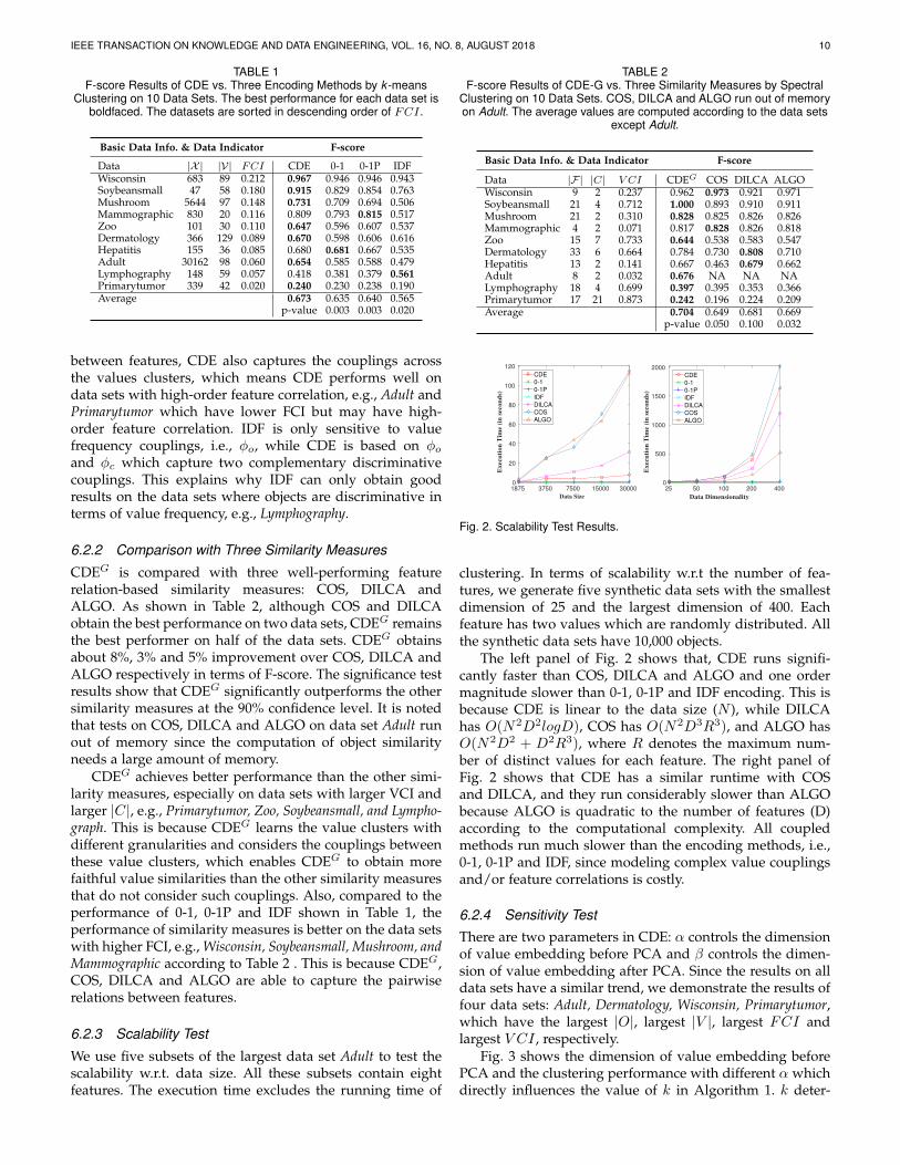
6.2.3 Scalability Test

We use five subsets of the largest data set Adult to test thescalability w.r.t. data size. All these subsets contain eightfeatures. The execution time excludes the running time of

TABLE 2F-score Results of CDE-G vs. Three Similarity Measures by Spectral

Clustering on 10 Data Sets. COS, DILCA and ALGO run out of memoryon Adult. The average values are computed according to the data sets

except Adult.

Basic Data Info. & Data Indicator F-score

Data |F| |C| V CI CDEG COS DILCA ALGOWisconsin 9 2 0.237 0.962 0.973 0.921 0.971Soybeansmall 21 4 0.712 1.000 0.893 0.910 0.911Mushroom 21 2 0.310 0.828 0.825 0.826 0.826Mammographic 4 2 0.071 0.817 0.828 0.826 0.818Zoo 15 7 0.733 0.644 0.538 0.583 0.547Dermatology 33 6 0.664 0.784 0.730 0.808 0.710Hepatitis 13 2 0.141 0.667 0.463 0.679 0.662Adult 8 2 0.032 0.676 NA NA NALymphography 18 4 0.699 0.397 0.395 0.353 0.366Primarytumor 17 21 0.873 0.242 0.196 0.224 0.209Average 0.704 0.649 0.681 0.669

p-value 0.050 0.100 0.032

1875 3750 7500 15000 30000

Data Size

0

20

40

60

80

100

120

Execu

tion

Tim

e (

in s

econ

ds)

CDE

0-1

0-1P

IDF

DILCA

COS

ALGO

25 50 100 200 400

Data Dimensionality

0

500

1000

1500

2000

Execu

tion

Tim

e (

in s

econ

ds)

CDE

0-1

0-1P

IDF

DILCA

COS

ALGO

Fig. 2. Scalability Test Results.

clustering. In terms of scalability w.r.t the number of fea-tures, we generate five synthetic data sets with the smallestdimension of 25 and the largest dimension of 400. Eachfeature has two values which are randomly distributed. Allthe synthetic data sets have 10,000 objects.

The left panel of Fig. 2 shows that, CDE runs signifi-cantly faster than COS, DILCA and ALGO and one ordermagnitude slower than 0-1, 0-1P and IDF encoding. This isbecause CDE is linear to the data size (N ), while DILCAhas O(N2D2logD), COS has O(N2D3R3), and ALGO hasO(N2D2 + D2R3), where R denotes the maximum num-ber of distinct values for each feature. The right panel ofFig. 2 shows that CDE has a similar runtime with COSand DILCA, and they run considerably slower than ALGObecause ALGO is quadratic to the number of features (D)according to the computational complexity. All coupledmethods run much slower than the encoding methods, i.e.,0-1, 0-1P and IDF, since modeling complex value couplingsand/or feature correlations is costly.

6.2.4 Sensitivity Test

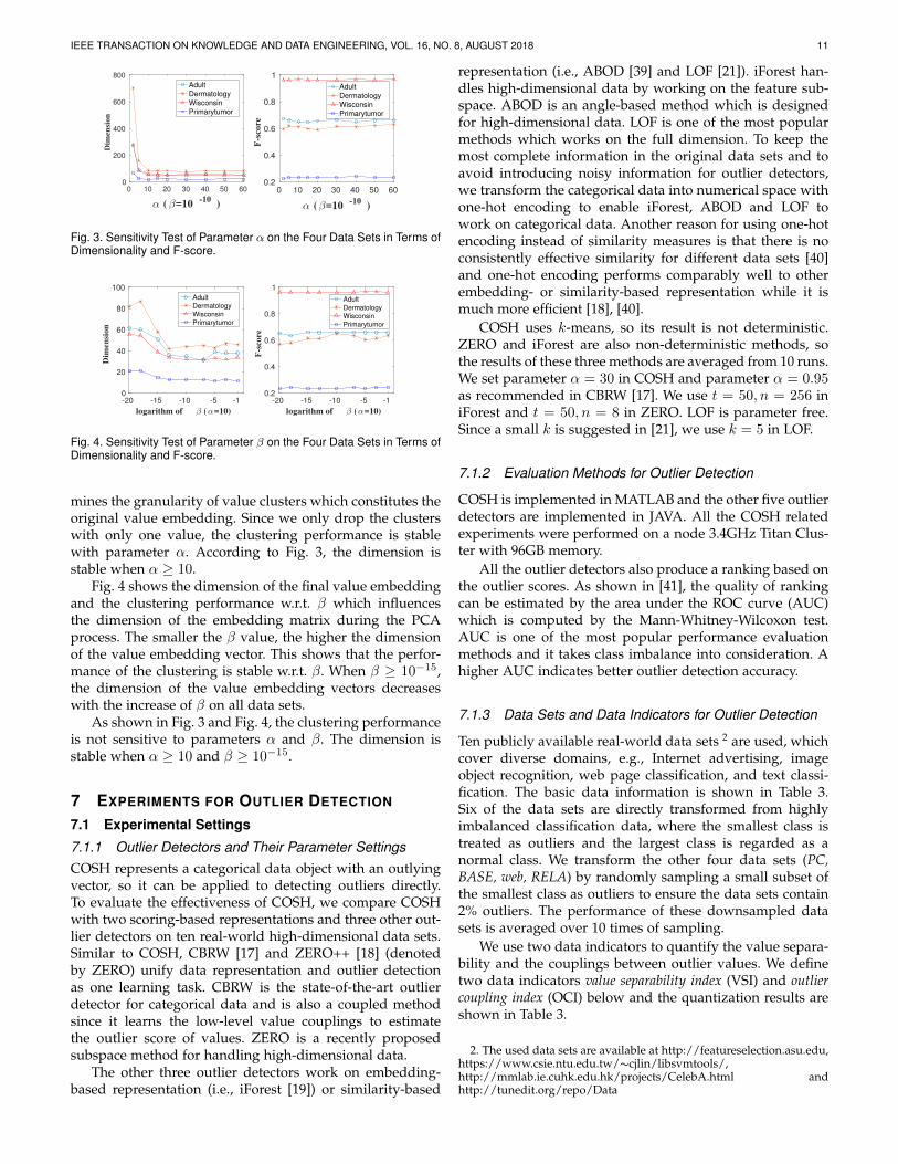
There are two parameters in CDE: α controls the dimensionof value embedding before PCA and β controls the dimen-sion of value embedding after PCA. Since the results on alldata sets have a similar trend, we demonstrate the results offour data sets: Adult, Dermatology, Wisconsin, Primarytumor,which have the largest |O|, largest |V |, largest FCI andlargest V CI , respectively.

Fig. 3 shows the dimension of value embedding beforePCA and the clustering performance with different α whichdirectly influences the value of k in Algorithm 1. k deter-


0 10 20 30 40 50 60

α (β=10-10

)

0

200

400

600

800

Dim

en

sio

n

Adult

Dermatology

Wisconsin

Primarytumor

0 10 20 30 40 50 60

α (β=10-10

)

0.2

0.4

0.6

0.8

1

F-s

co

re

Adult

Dermatology

Wisconsin

Primarytumor

Fig. 3. Sensitivity Test of Parameter α on the Four Data Sets in Terms ofDimensionality and F-score.

-20 -15 -10 -5 -1

logarithm of β (α=10)

0

20

40

60

80

100

Dim

en

sio

n

Adult

Dermatology

Wisconsin

Primarytumor

-20 -15 -10 -5 -1

logarithm of β (α=10)

0.2

0.4

0.6

0.8

1

F-s

co

re

Adult

Dermatology

Wisconsin

Primarytumor

Fig. 4. Sensitivity Test of Parameter β on the Four Data Sets in Terms ofDimensionality and F-score.

mines the granularity of value clusters which constitutes theoriginal value embedding. Since we only drop the clusterswith only one value, the clustering performance is stablewith parameter α. According to Fig. 3, the dimension isstable when α ≥ 10.

Fig. 4 shows the dimension of the final value embeddingand the clustering performance w.r.t. β which influencesthe dimension of the embedding matrix during the PCAprocess. The smaller the β value, the higher the dimensionof the value embedding vector. This shows that the perfor-mance of the clustering is stable w.r.t. β. When β ≥ 10−15,the dimension of the value embedding vectors decreaseswith the increase of β on all data sets.

As shown in Fig. 3 and Fig. 4, the clustering performanceis not sensitive to parameters α and β. The dimension isstable when α ≥ 10 and β ≥ 10−15.

7 EXPERIMENTS FOR OUTLIER DETECTION

7.1 Experimental Settings

7.1.1 Outlier Detectors and Their Parameter SettingsCOSH represents a categorical data object with an outlyingvector, so it can be applied to detecting outliers directly.To evaluate the effectiveness of COSH, we compare COSHwith two scoring-based representations and three other out-lier detectors on ten real-world high-dimensional data sets.Similar to COSH, CBRW [17] and ZERO++ [18] (denotedby ZERO) unify data representation and outlier detectionas one learning task. CBRW is the state-of-the-art outlierdetector for categorical data and is also a coupled methodsince it learns the low-level value couplings to estimatethe outlier score of values. ZERO is a recently proposedsubspace method for handling high-dimensional data.

The other three outlier detectors work on embedding-based representation (i.e., iForest [19]) or similarity-based

representation (i.e., ABOD [39] and LOF [21]). iForest han-dles high-dimensional data by working on the feature sub-space. ABOD is an angle-based method which is designedfor high-dimensional data. LOF is one of the most popularmethods which works on the full dimension. To keep themost complete information in the original data sets and toavoid introducing noisy information for outlier detectors,we transform the categorical data into numerical space withone-hot encoding to enable iForest, ABOD and LOF towork on categorical data. Another reason for using one-hotencoding instead of similarity measures is that there is noconsistently effective similarity for different data sets [40]and one-hot encoding performs comparably well to otherembedding- or similarity-based representation while it ismuch more efficient [18], [40].

COSH uses k-means, so its result is not deterministic.ZERO and iForest are also non-deterministic methods, sothe results of these three methods are averaged from 10 runs.We set parameter α = 30 in COSH and parameter α = 0.95as recommended in CBRW [17]. We use t = 50, n = 256 iniForest and t = 50, n = 8 in ZERO. LOF is parameter free.Since a small k is suggested in [21], we use k = 5 in LOF.

7.1.2 Evaluation Methods for Outlier Detection

COSH is implemented in MATLAB and the other five outlierdetectors are implemented in JAVA. All the COSH relatedexperiments were performed on a node 3.4GHz Titan Clus-ter with 96GB memory.

All the outlier detectors also produce a ranking based onthe outlier scores. As shown in [41], the quality of rankingcan be estimated by the area under the ROC curve (AUC)which is computed by the Mann-Whitney-Wilcoxon test.AUC is one of the most popular performance evaluationmethods and it takes class imbalance into consideration. Ahigher AUC indicates better outlier detection accuracy.

7.1.3 Data Sets and Data Indicators for Outlier Detection

Ten publicly available real-world data sets 2 are used, whichcover diverse domains, e.g., Internet advertising, imageobject recognition, web page classification, and text classi-fication. The basic data information is shown in Table 3.Six of the data sets are directly transformed from highlyimbalanced classification data, where the smallest class istreated as outliers and the largest class is regarded as anormal class. We transform the other four data sets (PC,BASE, web, RELA) by randomly sampling a small subset ofthe smallest class as outliers to ensure the data sets contain2% outliers. The performance of these downsampled datasets is averaged over 10 times of sampling.

We use two data indicators to quantify the value separa-bility and the couplings between outlier values. We definetwo data indicators value separability index (VSI) and outliercoupling index (OCI) below and the quantization results areshown in Table 3.

2. The used data sets are available at http://featureselection.asu.edu,https://www.csie.ntu.edu.tw/∼cjlin/libsvmtools/,http://mmlab.ie.cuhk.edu.hk/projects/CelebA.html andhttp://tunedit.org/repo/Data


• VSI is quantified by the value overlapping in normalobjects and outlier objects, defined as follows:

V SI = min |x|x ∈ Xn ∩ vxj ∈ V

Xoj |

|Xn|, j ∈ F, (18)

where Xn is the set of normal objects and Xo is the setof outlier objects, and vxj denotes the value of object x infeature j. A larger VSI indicates a weaker separabilityof values.

• The OCI is quantified by the pointwise mutual informa-tion between outlier values and normal values, whichis defined as follows:

OCI =pmi(vo, v

′o)

pmi(vo, v′o) + pmi(vo, vn), (19)

where pmi(vo, v′o) is the averaged pointwise mutual

information within outlier values, which is calculatedby pmi(vo, v

′o) = average p(vo,v

′o)

p(vo)p(v′o), vo, v

′o ∈ Vo.

OCI > 0.5 indicates that the couplings within outliervalues are stronger than the couplings between outliervalues and normal values.

7.2 Evaluation Results7.2.1 Outlier Detection EffectivenessThe AUC performance of COSH and its five competitors:CBRW, ZERO, iForest, ABOD and LOF is reported in Table3. COSH performs better than its five competitors on sevendata sets, and significantly outperforms them at the 95%confidence level. On average, COSH obtains more than 17%,27%, 39%, 29% and 44% improvement over CBRW, ZERO,iForest, ABOD and LOF, respectively. Of all the outlierdetection methods, COSH, CBRW and ZERO are scoring-based representation since they integrate model learningand data representation into representation, while iForest,ABOD and LOF are outlier detectors based on embeddingrepresentation. From Table 3, the performance of scoring-based representation is much better than pure outlier detec-tors that rely on data conversion.

In Table 3, the data sets are sorted in the descendingorder of V SI . The data indicator V SI describes the sep-arability of values from a single feature according to theoverlapping values of outlier objects and normal objects.COSH obtains the best performance on all the data sets withhigher V SI (e.g. V SI > 60%), and it achieves, on average,substantial AUC improvement over its five competitorsCBRW, ZERO, iForest, ABOD and LOF by more than 28%,46%, 67%, 50% and 30%, respectively. V SI quantifies theseparability of a single feature, while some outliers could beidentified by multiple features. COSH captures high-ordercouplings through value-cluster couplings, which helps todetect outliers in data sets without strongly coupled features(i.e., low VSI).

OCI captures the couplings between outliers and nor-mal values across two features. The larger OCI is, thestronger the couplings which exist within outliers and theweaker the couplings between outliers and normal objects.In the data sets with the highest OCI , i.e., w7a, COSHachieves much better performance than the others, whereasCOSH does not show its superiority in the data sets withthe lowest OCI , i.e., Cal28.

TABLE 3AUC Results of COSH vs. Five Outlier Detectors on 10 Data Sets.

Note: CBRW runs out of memory on high-dimensional data WebKB andReuters8. ABOD runs out-of-memory on large data w7a and CelebA

Data Info. Data Indicator AUC Performance

Data |X | |F| VSI OCI COSH CBRW ZERO iForest ABOD LOFw7a 49749 300 0.950 0.589 0.835 0.646 0.538 0.404 NA 0.500CelebA 202599 39 0.845 0.501 0.716 0.646 0.538 0.404 NA 0.500WebKB 1658 6601 0.814 0.551 0.753 NA 0.698 0.678 0.670 0.825RELATHE 794 4080 0.788 0.501 0.896 0.701 0.605 0.556 0.569 0.743BASEHOCK 1019 4320 0.706 0.513 0.909 0.618 0.529 0.471 0.488 0.664PCMAC 1002 3039 0.698 0.536 0.890 0.633 0.528 0.476 0.490 0.620Reuters8 3974 9467 0.260 0.552 0.872 NA 0.883 0.839 0.786 0.892Caltech-28 829 727 0.088 0.500 0.943 0.960 0.954 0.934 0.927 0.439Caltech-16 829 253 0.054 0.510 0.996 0.993 0.988 0.972 0.977 0.388wap.wc 346 4229 0.038 0.534 0.975 0.790 0.657 0.579 0.524 0.516Average 0.879 0.748 0.692 0.631 0.679 0.609

p-value 0.023 0.020 0.002 0.008 0.010

0.625 0.125 0.25 0.5 1 2 x105

Data Size

100

101

102

103

Execu

tion

Tim

e (

tim

es

w.r

.t. b

asi

c)

COE

CBRW

ZERO

iForest

ABOD

LOF

125 250 500 1000 2000 4000 8000

Data Dimensionality

100

101

102

103

104

Execu

tion

Tim

e (

tim

es

w.r

.t. b

asi

c)

COE

CBRW

ZERO

iForest

ABOD

LOF

Fig. 5. Scalability Test Results. ABOD and CBRW run out of memorywhen the number of objects reaches 25,000 and the number of featuresreaches 8,000, respectively

7.2.2 Scalability Test

COSH is implemented in MATLAB while the other methodsare implemented in JAVA, so the absolute time is not com-parable. We demonstrate the ratio of the execution time tothe base time which is from the smallest data set. We use sixsubsets of the largest data set CelebA to test the scalabilityw.r.t. data size. All these data sets contain the same numberof features, i.e., 39. The execution time on the smallest dataset is: 26.6s for COSH, 0.344s for CBRW, 3.416s for ZERO,0.299s for iForest, 3685.467s for ABOD, and 2.439s for LOF.

In terms of scalability w.r.t. the number of features, sevensubsets of the data sets with the largest number of features,R8 are used. All these seven data sets contain the samenumber of objects, i.e., 3,974. The execution time on thesmallest data set is: 88.21s for COSH, 1.657s for CBRW,7.244s for ZERO, 0.182s for iForest, 84.345s for ABOD, and0.581s for LOF.

The computational complexities of CBRW, ZERO, iFor-est, ABOD and LOF are O(ND2), O(ND), O(ND),O(N3D) and O(N2D) respectively. As shown in the rightpanel of Fig. 5, COSH is one of the most efficient methodscompared with other state-of-the-art outlier detection meth-ods w.r.t. the number of objects, since COSH is linear to thedata size and quadratic to the number of features. In theleft panel of Fig. 5, COSH and CBRW have similar runtimeand they run considerably slower than the other four de-tectors, since both COSH and CBRW capture complex valuecouplings while the other methods ignore them. AlthoughCOSH and CBRW run slower, they obtain significantlybetter AUC performance than their competitors, as shownin Table 3.


10 20 30 40 50 60

0.6

0.8

1

AU

C

w7a

10 20 30 40 50 60

0.6

0.8

1

AU

C

CelebA

10 20 30 40 50 60

0.6

0.8

1

AU

C

WebKB

10 20 30 40 50 60

0.6

0.8

1

AU

C

RELATHE

10 20 30 40 50 60

0.6

0.8

1

AU

C

BASEHOCK

10 20 30 40 50 60

0.6

0.8

1

AU

C

PCMAC

10 20 30 40 50 60

0.6

0.8

1

AU

C

Reuters8

10 20 30 40 50 60

0.6

0.8

1

AU

C

Caltech-28

10 20 30 40 50 60

0.6

0.8

1

AU

C

Caltech-16

10 20 30 40 50 60

0.6

0.8

1A

UC

wap.wc

Fig. 6. Sensitivity Test Results w.r.t. α on Ten Data Sets.

7.2.3 Sensitivity TestWe investigate the sensitivity test of COSH w.r.t. its onlyparameter α on all the 10 data sets using a wide range ofα, i.e., 10, 20, 30, 40, 50, 60. The sensitivity test results ofCOSH are shown in Fig. 6. COSH performs stably w.r.t.α on all data sets. The larger α means the less number ofclustering times and a smaller number of value clusters.

8 DISCUSSIONS

CURE is a hierarchical framework which can be customizedfrom multiple levels. We instantiate CURE by customizingthe value cluster learning and coupling learning betweenvalue clusters according to different applications based onthe same coupling functions. More instances may be derivedby capturing other forms or levels of couplings [6] forspecific applications.

The two complementary coupling functions used byCDE and COSH capture only pairwise couplings. Instanti-ating CURE by incorporating arbitrary length patterns andtheir couplings may improve the discriminative ability ofthe low-level value coupling functions, and further improvethe representation quality.

One important CURE component is the value clusterlearning, which is instantiated by k-means clustering in CDEand COSH. Although k-means has multiple advantages, ithas some limitations for detecting the special shape of clus-ters and overlapping clusters. Learning arbitrary shapes ofvalue clusters with different clustering methods may enrichthe information of value clusters. However, various kinds ofvalue clusters may induce more heterogeneous couplings ornoises. Therefore, more advanced methods may be requiredto capture couplings between value clusters in this case.

Another important part of CURE is the coupling learn-ing between value clusters, which is highly related to theproperties of value clusters. There may be various formsof couplings between value clusters, which are also hardto capture and interpret. Incorporating more sophisticatedmethods to learn explicit and implicit complex value cou-plings, e.g., by deep models, may be explored to improvethe utility of each value cluster.

9 CONCLUSIONS AND FUTURE WORK

This paper proposes a novel unsupervised representationframework (CURE) for categorical data which models hier-archical value couplings in terms of feature value couplings

and value cluster couplings. Instantiating CURE, CDE andCOSH are respectively introduced for clustering and outlierdetection, which are based on two complementary and dis-criminative value couplings. A contrastive analysis of CDEand COSH explains the contrasting instantiation capabilityof CURE.

Different from existing encoding-based embedding andfeature correlation-based similarity measures, CDE learnsthe data embedding from value clusters w.r.t. couplingswithin and between value clusters. Extensive experimentsshow that (1) CDE significantly outperforms typical em-bedding methods and similarity measures for clustering;(2) two data indicators can facilitate the explanation ofclustering performance on complex data sets; (3) CDE hasgood scalability and is more efficient than similarity-basedrepresentation; and (4) CDE performance is insensitive tothe two parameters.

Different from existing single-granular outlier detectionmethods, COSH observes hierarchical outlying behaviorsfrom value-to-value clusters with different granularities.Extensive experiments show that (1) COSH significantlyoutperforms five state-of-the-art outlier detection methods.(2) Two data indicators can facilitate the explanation ofoutlier detection on complex data sets. (3) COSH has a goodscalability which suits high-dimensional data sets. (4) Thereis only one parameter in COSH and it has little influence onthe outlier detection performance.

As discussed, there are great opportunities to furtherexpand CURE for different learning tasks and scenarios withcomplex coupling relationships.

ACKNOWLEDGMENTS

This work is partially supported by the The Na-tional Key Research and Development Program of China(2016YFB0200401) by program for New Century Excel-lent Talents in University by National Science Foundation(NSF) China 61402492, 61402486, 61379146, by the HUNANProvince Science Foundation 2017RS3045, and by the ChinaScholarship Council (CSC Student ID 201603170310).

REFERENCES

[1] L. Cao, “Non-iidness learning in behavioral and social data,” TheComputer Journal, vol. 57, no. 9, pp. 1358–1370, 2014.

[2] C. Wang, X. Dong, F. Zhou, L. Cao, and C.-H. Chi, “Coupledattribute similarity learning on categorical data,” IEEE TNNLS,vol. 26, no. 4, pp. 781–797, 2015.

[3] S. Jian, L. Cao, K. Lu, and H. Gao, “Unsupervised coupled metricsimilarity for non-iid categorical data,” IEEE TKDE, 2018.

[4] C. Zhu, L. Cao, Q. Liu, J. Yin, and V. Kumar, “Heterogeneousmetric learning of categorical data with hierarchical couplings,”IEEE TKDE, 2018.

[5] L. Cao, Y. Ou, and S. Y. Philip, “Coupled behavior analysis withapplications,” IEEE TKDE, vol. 24, no. 8, pp. 1378–1392, 2012.

[6] L. Cao, “Coupling learning of complex interactions,” InformationProcessing & Management, vol. 51, no. 2, pp. 167–186, 2015.

[7] Y. Bengio, A. Courville, and P. Vincent, “Representation learning:A review and new perspectives,” IEEE TPAMI, vol. 35, no. 8, pp.1798–1828, 2013.

[8] A. Foss and O. R. Zaıane, “A parameterless method for efficientlydiscovering clusters of arbitrary shape in large datasets,” in Pro-ceedings of ICDM. IEEE, 2002, pp. 179–186.

[9] A. Aizawa, “An information-theoretic perspective of tf–idf mea-sures,” Information Processing & Management, vol. 39, no. 1, pp.45–65, 2003.


[10] A. Ahmad and L. Dey, “A method to compute distance betweentwo categorical values of same attribute in unsupervised learningfor categorical data set,” Pattern Recognition Letters, vol. 28, no. 1,pp. 110–118, 2007.

[11] D. Ienco, R. G. Pensa, and R. Meo, “From context to dis-tance: Learning dissimilarity for categorical data clustering,” ACMTKDD, vol. 6, no. 1, p. 1, 2012.

[12] H. Jia, Y.-m. Cheung, and J. Liu, “A new distance metric forunsupervised learning of categorical data,” IEEE Transactions onNeural Networks and Learning Systems, vol. 27, no. 5, pp. 1065–1079,2016.

[13] Z. He, X. Xu, Z. J. Huang, and S. Deng, “FP-outlier: Frequentpattern based outlier detection,” Computer Science and InformationSystems, vol. 2, no. 1, pp. 103–118, 2005.

[14] L. Akoglu, H. Tong, J. Vreeken, and C. Faloutsos, “Fast and reliableanomaly detection in categorical data,” in Proceedings of CIKM.ACM, 2012, pp. 415–424.

[15] M. E. Otey, A. Ghoting, and S. Parthasarathy, “Fast distributedoutlier detection in mixed-attribute data sets,” DMKD, vol. 12, no.2-3, pp. 203–228, 2006.

[16] F. Angiulli, F. Fassetti, and L. Palopoli, “Detecting outlying proper-ties of exceptional objects,” ACM Transactions on Database Systems,vol. 34, no. 1, p. 7, 2009.

[17] G. Pang, L. Cao, and L. Chen, “Outlier detection in complexcategorical data by modelling the feature value couplings,” inProceedings of IJCAI. AAAI Press, 2016, pp. 1902–1908.

[18] G. Pang, K. M. Ting, D. Albrecht, and H. Jin, “ZERO++: Harness-ing the power of zero appearances to detect anomalies in large-scale data sets,” Journal of Artificial Intelligence Research, vol. 57, pp.593–620, 2016.

[19] F. T. Liu, K. M. Ting, and Z.-H. Zhou, “Isolation-based anomalydetection,” ACM TKDD, vol. 6, no. 1, p. 3, 2012.

[20] H.-P. Kriegel and A. Zimek, “Angle-based outlier detection inhigh-dimensional data,” in Proceedings of SIGKDD. ACM, 2008,pp. 444–452.

[21] M. M. Breunig, H.-P. Kriegel, R. T. Ng, and J. Sander, “LOF:identifying density-based local outliers,” in ACM sigmod record,vol. 29, no. 2. ACM, 2000, pp. 93–104.

[22] J. Cohen, P. Cohen, S. G. West, and L. S. Aiken, Applied multipleregression/correlation analysis for the behavioral sciences. Routledge,2013.

[23] Y. Bengio, Y. LeCun et al., “Scaling learning algorithms towardsai,” Large-scale kernel machines, vol. 34, no. 5, pp. 1–41, 2007.

[24] I. Jolliffe, Principal component analysis. Wiley Online Library, 2002.[25] S. Deerwester, S. T. Dumais, G. W. Furnas, T. K. Landauer, and

R. Harshman, “Indexing by latent semantic analysis,” Journal ofthe American Society for Information Science, vol. 41, no. 6, p. 391,1990.

[26] D. M. Blei, A. Y. Ng, and M. I. Jordan, “Latent dirichlet allocation,”JMLR, vol. 3, no. Jan, pp. 993–1022, 2003.

[27] T. Mikolov, K. Chen, G. Corrado, and J. Dean, “Efficient esti-mation of word representations in vector space,” arXiv preprintarXiv:1301.3781, 2013.

[28] T. Hofmann, “Probabilistic latent semantic indexing,” in Proceed-ings of SIGIR. ACM, 1999, pp. 50–57.

[29] A. T. Wilson and P. A. Chew, “Term weighting schemes for latentdirichlet allocation,” in The 2010 Annual Conference of the NorthAmerican Chapter of the Association for Computational Linguistics.Association for Computational Linguistics, 2010, pp. 465–473.

[30] T. Mikolov, I. Sutskever, K. Chen, G. S. Corrado, and J. Dean,“Distributed representations of words and phrases and their com-positionality,” in Proceedings of NIPS, 2013, pp. 3111–3119.

[31] T. F. Cox and M. A. Cox, Multidimensional Scaling. CRC press,2000.

[32] G. E. Hinton and S. T. Roweis, “Stochastic neighbor embedding,”in Proceedings of NIPS, 2002, pp. 833–840.

[33] K. Zhang, Q. Wang, Z. Chen, I. Marsic, V. Kumar, G. Jiang,and J. Zhang, “From categorical to numerical: Multiple transitivedistance learning and embedding,” in Proceedings of SDM. SIAM,2015.

[34] J. Song, C. Zhu, W. Zhao, W. Liu, and Q. Liu, “Model-awarerepresentation learning for categorical data with hierarchical cou-plings,” in International Conference on Artificial Neural Networks.Springer, 2017, pp. 242–249.

[35] S. Wu and S. Wang, “Information-theoretic outlier detection forlarge-scale categorical data,” IEEE TKDE, vol. 25, no. 3, pp. 589–602, 2013.

[36] P. A. Estevez, M. Tesmer, C. A. Perez, and J. M. Zurada, “Nor-malized mutual information feature selection,” IEEE TNN, vol. 20,no. 2, pp. 189–201, 2009.

[37] D. M. Powers, “Evaluation: from precision, recall and f-measureto roc, informedness, markedness and correlation,” 2011.

[38] L. Yu and H. Liu, “Feature selection for high-dimensional data: Afast correlation-based filter solution,” in Proceedings of ICML, vol. 3,2003, pp. 856–863.

[39] H.-P. Kriegel, A. Zimek et al., “Angle-based outlier detection inhigh-dimensional data,” in Proceedings of SIGKDD. ACM, 2008,pp. 444–452.

[40] S. Boriah, V. Chandola, and V. Kumar, “Similarity measures forcategorical data: A comparative evaluation,” red, vol. 30, no. 2,p. 3, 2008.

[41] D. J. Hand and R. J. Till, “A simple generalisation of the area underthe roc curve for multiple class classification problems,” Machinelearning, vol. 45, no. 2, pp. 171–186, 2001.

Songlei Jian Songlei Jian is currently work-ing toward a Ph.D. degree, jointly supervised atthe National University of Defense Technology,China and the University of Technology Sydney,Australia. Her research interests include datarepresentation, unsupervised learning and com-plex network analysis.

Guansong Pang Guansong Pang is a PhD can-didate in the Advanced Analytics Institute at theUniversity of Technology Sydney. Before joiningAAI, he received a Master of Philosophy in datamining from Monash University. His research in-terests include data mining and non-IID learning.

Longbing Cao Longbing Cao is a Professor atthe University of Technology Sydney. He has aPhD in Pattern Recognition and Intelligent Sys-tems and another in Computing Sciences. Hisresearch interests include data science, analyt-ics and machine learning, and behavior informat-ics and their enterprise applications.

Kai Lu Kai Lu is a Professor and the DeputyDean of the College of Computer Science, Na-tional University of Defense Technology, China.His research interests include parallel and dis-tributed system software, operating systems,and big data analytics.

Hang Gao Hang Gao is a Ph.D. graduate of Na-tional University of Defense Technology, China.His research interests include machine learning,data analytics and mining.

ieee transaction on knowledge and data engineering, … · expressive numerical representation of...

Documents