ieee transactions on geoscience and …web.unbc.ca/~dkang/index_files/tgrs-kang-2169073-x.pdfyear...

IEEE TRANSACTIONS ON GEOSCIENCE AND REMOTE SENSING 1

Observing System Simulation of Snow MicrowaveEmissions Over Data Sparse Regions—

Part I: Single Layer PhysicsDo Hyuk Kang and Ana P. Barros, Senior Member, IEEE

Abstract—The objective of this work is to develop a frame-work for monitoring snow water equivalent (SWE) and snowpackradiometric properties (e.g. surface emissivity and reflectivity)and microwave emissions in remote regions where ancillary dataand ground-based observations for model calibration and/or dataassimilation are lacking. For this purpose, an existing land surfacehydrology model (LSHM) [1] with single-layer (SL) snow physicswas coupled to a microwave emission model (MEMLS, [2], [3]).The coupled model (MLSHM-SL) predicts microwave emissionsat various frequencies and polarizations as well as snowpackradiometric properties (e.g. emissivity) based on snowpack den-sity, temperature, snow depth, and volumetric liquid water con-tent simulated by the hydrology model with atmospheric forcingobtained from either observations, or the analysis of weatherforecasts. The MLSHM-SL was evaluated in prognostic observingsystem simulation (OSS) mode for two case-studies: 1) a multi-year simulation of snowpack radio-brightness behavior at Valdai,Russia compared against scanning multichannel microwaveradiometer (SMMR) observations at three frequencies (18,21, and 37 GHz, V, and H polarizations) over six years,1978–1983; and 2) an intercomparison of simulated and ob-served brightness temperatures for the special sensor microwaveimager (SSM/I) and the advanced microwave scanning ra-diometer-EOS (AMSR-E) during the 2002–2003 snow seasonas part of CLPX (cold land processes field experiment) inColorado. In the case of Valdai, the model captures well themass balance as well as radiometric behavior of the snowpackduring both accumulation and melt, with significantly best skillfor vertical polarization (10–16 K differences in error statistics ascompared to horizontal polarization), particularly in the winterseason January–March (dry snow conditions). Larger biases weredetected for intermittent snowpack conditions at the beginning ofthe fall season due to uncertainty in fractional snow cover andsnow wetness at the spatial scale of the SMMR. Similar resultswere obtained for the OSS of SSM/I and AMSR-E for CLPX,though differences between vertical and horizontal polarizationerror statistics are more modest (∼2–4 K). Error statistics arelower for AMSR-E V-pol at 19 and 37 GHz. MLSHM-SL pre-dicted snowpack physical properties (bulk snow density and SWE)compare well against CLPX snowpit observations during the ac-cumulation season with residuals smaller than 10% of observed

Manuscript received November 30, 2010; revised May 28, 2011 andAugust 19, 2011; accepted September 11, 2011. This research was supportedin part by a NASA Earth System Science Fellowship with the first author, andNASA Grant NNX07AK40G and NOAA Grant NA080AR4310701 with thesecond author.

The authors are with the Pratt School of Engineering, Duke University,Durham, NC 27708 USA (e-mail: [email protected]).

Color versions of one or more of the figures in this paper are available onlineat http://ieeexplore.ieee.org.

Digital Object Identifier 10.1109/TGRS.2011.2169073

values. Moreover, the MLSHM-SL simulations in full prognosticmode, and without calibration from the beginning through theend of the snow season, are as skillful as MEMLS with specifiedphysical attributes from snow pit observations. This indicates thatthe MSLSHM-SL can be used independently as a physically basedestimator of SWE in remote regions, and in a data-assimilationframework to provide a physical basis to the interpretation ofsatellite-based observations of snow.

Index Terms—Electromagnetic propagation in absorbing me-dia, nonhomogeneous media, single-layer, snow hydrology.

LIST OF SYMBOLS

LSHM (input and output)

Ka air heat conductivity [W/K m]ρa air density [kg/m3]Qsn amount of heat used to melt the snowpack [J]Δhk

sm amount of snowmelt at the kth layer [m]ρw density of water [kg/m3]εs bulk emissivity at the snowpack atmosphere interfaceiwk ice water content at the kth layer [m]LWCk liquid water content in the kth layer [m]ρks snow density in the kth layer [kg/m3]C∗

sn depth-adjusted snow fractional areaKk

sn snow heat conductivity in the kth layer [W/K m]hkswe snow water equivalent in the kth layer [m]

hksn snow depth of the kth layer [m]

Φsn snowmelt outflux [m/s]Ks soil heat capacity [W/K m]c∗ heat capacity of snow [J/kg K]ci heat capacity of ice [J/kg K]Cp heat capacity of air at the constant pressure [J/kg K]hksn snow depth at the kth layer [m]

Kksn heat conductivity of snow in the kth layer [W/kg K]

FR net solar radiation [W/m2]Fs net solar radiation [W/m2]Lh latent heat flux [W/m2]Ps snow weight pressure [N/m2]qa specific humidity of airqsat saturated humidity of snowpackSh sensible heat flux [W/m2]T1 temperature measured in the reference height [K]Ta air temperature [K]To soil temperature [K]Te equivalent temperature for melting [K]Ti melting temperature [K]

0196-2892/$26.00 © 2011 IEEE

2 IEEE TRANSACTIONS ON GEOSCIENCE AND REMOTE SENSING

T ks snow temperature at the kth layer [K]

To soil temperature [K]Psn snowfall precipitation [kg/(sec m2)]xPr rainfall precipitation [kg/(sec m2)]

MEMLS (input)

Ak ∼ Dk brightness temperature inside the snow layer k = 1to n [K]

γa absorption coefficient [1/m]γc combination effect from scattering and absorption

coefficient [1/m]ε effective permittivity of wet snowε′′i imaginary part of permittivity of icen′′ imaginary part of refractive index of internal

snowpacksj interface reflectance between j and j + 1 layersγb scattering coefficient [1/m]e emissivity of internal snowpackeback emissivity of internal snowpack backwardly calcu-

lated from Ts and Tb

f frequency used for a passive microwave radiometerpec snow grain size correlation length [mm]r reflectivity of internal snowpackt transmissivity of internal snowpackTb brightness temperature [K]Tsim simulated brightness temperature just after the

snowpack surface [K]Tsky sky downwelling radiation [K]

Atmospheric Correction (input and output)

τ atmospheric optical depth [neper]e atmospheric emissivityes snowpack surface emissivity generated from MEMLS

routine []L vertical liquid water [mm]r atmospheric reflectivityta atmospheric transmissivityTapp Apparent brightness temperature approximated at ra-

diometer [K]Tappm Apparent brightness temperature locally approximated

at radiometer [K]Tsim simulated brightness temperature before atmospheric

correction [K]V precipitable water [mm]Af intercept of linear fit on optical depth with V and L

[neper]Bf coefficient of V in linear fit on optical depth with V

and L [neper/mm]Df coefficient of L in linear fit on optical depth with V

and L [neper/mm]

Other

μ the cosine of the incidence angleC3, C4, C5 and C6 are constants for compaction rate

equation.SSA specific surface areaΔT difference between microwave

emissions of vertical and horizontalpolarization

κa absorption coefficient of atmosphere[dB/m]

κe extinction coefficient of atmosphere[dB/m]

I. INTRODUCTION

SNOWFALL, snow accumulation, and snow cover extentvary with weather and climate regime, continental versus

marine environments, land cover and land use, and landformand elevation. Where present, snow cover controls the terrestrialenergy budget in the cold season, and snowmelt available forinfiltration and runoff in the warm season governs the waterbudget of large regions [6]. Approaches to monitor snow accu-mulation include in situ measurements, passive/active remotesensing, and operational systems combining snow hydrology,snow microphysics, radiative transfer, and data assimilationto integrate models and observations. Ground-based, in situsnowpack observations have relied traditionally on direct phys-ical measurements from snow pit, snow pillows, and snowcores [7]. Recently, new instrumentation has been introduced tomonitor snow cover and snow water content indirectly withoutdisturbing the snowpack such as time domain reflectometry [8](TDR), ground penetrating radar [9]–[11], and active L-bandsensing [12]. Whereas the integration of TDR and L-bandsensors into wireless networks anticipates the possibility ofground-based sensing at high spatial resolution, satellite-basedremote sensing is necessary to cover large continental areas andfor the long-time scales needed for climate research and forwater resources applications.

Satellite-based microwave passive remote sensors particu-larly apt for the retrieval of snow states are the scanningmultichannel microwave radiometer (SMMR, 1979–1987), thespecial sensor microwave imager (SSM/I, 1987–present), andmore recently the advanced microwave scanning radiometer-earth observing system (EOS) (AMSR-E). Snow cover, snowdepth (SD), snow wetness estimated (retrieved) from SMMR,SSM/I, and AMSR-E observations have been widely usedto characterize northern hemisphere snow cover ([13]–[16],among many others). Generally, retrieval algorithms can be di-vided in two major classes: 1) empirical algorithms (e.g. [17]);and 2) physically based algorithms, or microwave emissionsimulators, consisting of radiative transfer (microwave emis-sion) models coupled to an optimal estimation algorithm toderive snow states from observed brightness temperatures atspecific frequencies (e.g. [18]). Prominent microwave emissionmodels for snow retrieval include the Helsinki University ofTechnology radiative transfer model (HUT) [19], [20], thedense media radiative transfer model (DMRT) [21]; and themicrowave emission model for multilayer snowpack (MEMLS)[2], [3]. These models have been evaluated against field ob-servations either independently e.g. [22] or integrated withvarious snow hydrology models operating at the field scale(e.g. [23]–[25] among others), and in the context of dedicatedfield campaigns such as cold land process field experiment[5] (CLPX). An intercomparison of electromagnetic modelsfor passive remote sensing of snow was conducted by [41],who found significant discrepancies among models depending

KANG AND BARROS: OBSERVING SYSTEM SIMULATION OF SNOW MICROWAVE EMISSIONS I 3

Fig. 1. Schematic view of grid resolutions of ERA40 (2.5◦ × 2.5◦) and SMMR (25× 25 km2) located in Valdai, Russia.

on frequency and polarization, and snowpack condition (type,wetness, and snow grain size) for various types of snow at thecoarse spatial resolution of current sensors (SSM/I and AMSR-E) and corresponding equal area scalable Earth (EASE)-Gridproducts such as snow water equivalent (SWE) and snowcover available from the National Snow and Ice Data Center(NSIDC) [60], [61]. In addition to snowpack condition, thesediscrepancies also result from the heterogeneity of atmosphericabsorption within the sensor footprint due to spatial variabilityof atmospheric moisture, and particularly atmospheric liquidwater content (LWC), and thus clouds and rainfall [32], [57]–[59]. Furthermore, heterogeneity associated with fractionalvegetation cover can introduce large bias at the spatial res-olution of EASE-grid products, particularly in the case ofdense forests [62]. The scattering signal of forest stands candominate the temporal evolution of the scattering signal of thesnowpack leading to loss of sensitivity to snow accumulationand snow microphysical changes. These effects decrease withthe decrease in forest density (vegetation volume) [63].

From the point of view of physical hydrology, and buildingon the pioneer work of [44], much effort has been placed intothe development of bulk models (single-layer (SL)) to trackthe evolution of the mass and energy balance of the snowpack[45]–[50] with two distinct types of hydrological applications inmind: 1) estimation of SWE for water resources applications;and 2) estimation of melt runoff and timing of melt. [26]proposed a 1-D vertical multilayer (ML) representation of thesnowpack that allows the temporal development of heteroge-neous layers due to accumulation during storm events, transientmelt and freeze cycles, rain-on-snow effects, and compactionand aging processes. Several variants of [26] have been imple-mented in the literature (e.g. [23], [24]).

The challenge in passive microwave remote sensing is theambiguity in the interpretation of areal radiometric tempera-tures in terms of representative snowpack physical properties,and specifically snow wetness and SWE, at the same spatialscale. The research presented here establishes a dynamicalmodeling framework for simulating the joint evolution of SWEand snow microwave emission. For this purpose, we rely on

a coupled snow hydrology-microwave emission modeling sys-tem that links an existing hydrology model, the land surfacehydrology model (LSHM) [1] to MEMLS [2], [3]. Hereafter,the coupled hydrology-emission model will be referred to asMLSHM. Operationally, such framework can either be usedas a prediction system to support physically based retrievalalgorithms, or for constraining direct data assimilation of radio-metric observations of snow conditions into forecasts models.

The coupled MLSHM was implemented using both SLand ML representations of the snowpack hydrology. In thismanuscript, Part 1, the coupled MLSHM retains the SL snowhydrology parameterization described by [1]. The hydrolog-ical and radiometric behaviors of the snowpack using theML formulation of the MLSHM are investigated separatelyin Part 2 [56]. The purpose of Part 1 is to demonstrate thatthe coupled model is a useful monitoring and predictive toolof the evolution of SWE in remote regions where groundobservations are sparse if at all available, atmospheric forcingmust be obtained from relatively coarse resolution numericalweather models, and thus satellite observations are the only dataavailable to evaluate model fidelity over time. The objectiveof Part 2 is to characterize the impact of ML snow physicsin the MLSHM’s ability to diagnose snowpack hydrologicstates and radiometric properties that can be used to predictthe onset of melt and transient structural and, or microphysicalchanges in the snowpack which are important for avalancheand snowmelt prediction on the one hand, and more gener-ally for estimating snowpack properties from remote sensingobservations. Following [55], the working premise is that theSL formulation addresses the question of snowpack bulk waterstorage, whereas the ML formulation addresses the questionof snowpack stability and condition, in addition to waterstorage.

In this manuscript, the coupled MLSHM-SL is evaluatedin observing system simulation (OSS) mode for two casestudies for very different climatic and physiographic regions:1) an intercomparison of a multi-year simulation of snowpackmicrowave behavior at Valdai, Russia, against SMMR observa-tions at three frequencies (18, 21, and 37 GHz H-pol and V-pol)


Fig. 2. Small regional study area for CLPX 2002 including the Fraser MSA, (mesocell study area, see inset) [http://nsidc.org/data/clpx/clpx_pits.html]. TheGBMR-7 (ground-based passive microwave radiometer-7) is located at the local scale observation station, local scale observation site (LSOS) marked above).There are three ISAs (intense study areas) within the Fraser MSA where several snow pit measurements are available as marked in the inset.

for a six year period, 1978–1983 (Fig. 1); and 2) an intercom-parison against SSM/I (19.35, 22.235, and 37.0 GHz H-poland V-pol) and AMSR-E (18.7, 23.8, and 36.5 GHz H-pol andV-pol) in Colorado during the 2002–2003 snow season as partof CLPX (Fig. 2). The motivation to select the Valdai case studywas twofold: 1) previously, the snow hydrology in the LSHMwas successfully evaluated for a 16-year simulation from 1966to 1983 using project for the intercomparison of land surfaceschemes (PILPS) data sets and without calibration [1], and2) Valdai can be viewed as typical of remote sites where limitedground-based ancillary data are available to force the hydrologymodel. The CLPX case study provides a means to evaluatethe skill of the coupled MLSHM-SL against a comprehensivedatabase of ground observations at meso- and point scales,as well as the opportunity to compare the simulated radio-metric behavior with observations from two different sensors,AMSR-E and SSM/I.

The manuscript is organized as follows. The modelingframework is described in Section II. Section III presentsan overview of all data sets including satellite observations,initial conditions and forcing data for the surface hydrologymodel, and data used for the atmospheric attenuation correctionalgorithm. The results for each case study are analyzed indetail and discussed in Section IV. Section V summarizesthe research and provides an overview of major results andconclusions.

II. MODEL DESCRIPTION

The model description presented here applies to the MLformulation of snow hydrology, and the SL implementationof the model is viewed as a particular case. A flow chartshowing the structure of the coupled MLSHM is shown inFig. 3. The LSHM output consists of SD hsn [m]; snowpackvolumetric liquid water content LWC [m]; snowpack ice watercontent iw [m]; snow density ρs [kg/m3]; SWE hswe [m] with(hswe = hsn × ρs/ρw) where ρw is the density of water; snowtemperature Ts [K]; and the snow correlation length pec [m]that is used to represent the modulation of volume scatteringin MEMLS by variations in snow grain size distribution. Anatmospheric correction algorithm that relies on a parameteri-zation of the optical depth τ of the atmosphere as a functionof atmospheric moisture profiles (water vapor and liquid water)is also implemented. The application of the LSHM implies theavailability of meteorological forcing (winds, air temperatureand relative humidity, surface pressure, precipitation) from alocal tower (Valdai), or from weather forecasting and analysis(CLPX, Valdai).

A. Land Surface Hydrology Model (LSHM)

The model domain of the 1-D LSHM column is composedof atmospheric boundary layer, ground surface (bare soil,


Fig. 3. Schematic view of the coupled MLSHM flow chart. Forcing: Ta—airtemperature, RHa—air relative humidity, Ua—wind speed, pa–surface pres-sure, Pr—rainfall, Psn—snowfall, SWin—incoming shortwave radiation,Lwin—incoming longwave radiation; LSHM snow hydrology output andMEMLS input : SD—snow depth (hsn), SWE—snow water equivalent (hswe),LWC–volumetric liquid water content, ρs—snow density, Ts—snowpack tem-perature; MEMLS output: T f

sim (same as T fb

) and ef—respectively simulatedbrightness temperature and emissivity at frequency f for H and V polarization;MLSHM output: T f

app—brightness temperature at the top of the atmosphere atfrequency f for H and V polarization.

snowpack, and canopy fractions), and a soil column. A com-plete description of the LSHM is presented in [1]. Here, thefocus is on the snow physics only. At the snowpack–atmosphereinterface, the boundary condition is the net surface energy flux

Φ(0, t) = FR(t)± Sh(t)± Lh(t) (1)

where FR is the net (shortwave plus longwave) radiation flux[W/m2], Sh is the sensible heat flux [W/m2], and Lh is the latentheat flux [W/m2]. The heat transfer equation between adjacentinternal layers is expressed by

c∗snρwhswe(z, t)∂Ts

∂t= Ksn

∂T

∂z+Q(z, t) + Φ(z, t), z > 0.

(2)

The heat exchange sources and sinks represented by Q(z, t)due to phase changes (freezing and melting) are dealt withseparately for each layer, and the forcing term is null [Φ(z, t) =0.0], except at the bottom of the snowpack where the boundarycondition is expressed by

Φ(z1, t) = Gh(t) = −Ks∂T0

∂zo. (3)

Here, hswe (z, t) is the SWE profile[m], Ts (z, t) is the snowtemperature profile, To is the temperature of the top soil layer atthe interface between the bottom layer of the snowpack and theground surface, c∗sn is the specific heat capacity of the snowpack[J/kg K], Gh is the ground heat flux (set to zero when thesoil is frozen), and Ksn (z) and Ks are, respectively, the heatconductivity of the snow and the top soil layer [W/(m K)].Equation (2) is resolved numerically using a forward-in-time,and centered-in-space, finite-difference vertical discretizationof the snowpack in n layers, with layer 1 at the bottom of the

snowpack adjacent to the soil, and layer n at the top adjacentto the atmospheric boundary layer. In the SL implementationn = k = 1. The heat conductivity of the snowpack is estimatedas per [20] and [53]

Ksn(z) =(Ka + 7.75× 10−5ρs(z) + 1.105

× 10−6 × (ρs(z))2)· (Ki −Ka) (4)

where Ka and Ki are the heat conductivities of air and ice,respectively.

A detailed description of the energy balance equations in-cluding estimation of net solar radiation, FR, sensible heatflux, Sh, and latent heat flux, Lh, are presented in [1]. Subgridscale heterogeneity due to the existence of bare soil, vegetation,and water ponds is treated in the LSHM by calculating theenergy and water budgets separately for each land-use/land-cover class, and subsequently a grid-scale representative valueis estimated based on the weighted averages of the values foreach class proportional to its fractional area [1]. For transferto MEMLS, two values of surface temperature are thereforeavailable: the grid-scale value, and the snowpack fractionvalue. Results from a study along a 10◦ latitude transect inQuebec, Canada by [63] suggest that the effect of vegetationfor fractional cover below 0.2–0.3 can be neglected. Becausethe version of MEMLS used here does not include a canopyemission model, and because the forest fractional remains doesnot exceed 0.1–0.2 for our applications during the most ofthe snow season, the temperature of the snowpack is used inMEMLS in the case studies described here.

Based on the update of snow temperature for each layer k,at time t, melting is initiated when T k

s exceeds the meltingtemperature, Ti (Ti = 273.15 K), and the heat flux Qk

sn =Csnciρsh

ksn(T

ks − Ti) is used to melt layer k (ci is the specific

heat of ice). As in [24] and [1], melting takes place in twostages: superficial and deep melting. The criterion is set basedon the equilibrium temperature Te

Te =T ks + C∗

sn

[(T k−1s − T k+1

s

)+

cic∗sn

(T ks − Ti

)](5)

C∗sn =Csn ·min

{1,

iwk

hksn

}. (6)

Light melting occurs when Te < Ti, in which case onlythe upper part of the layer melts to subsequently refreeze.Deep melting occurs when Te > Ti and affects the entire layerleading to a change in SD

Δhksn = min

{hksn,

ciρksh

ksn

(T ks − Ti

)Lmρw

}(7)

where Lm is the specific heat for fusion for ice. The volumetricLWC, lwk, is the amount of volumetric liquid water that isretained in the kth layer of the snowpack, and the snowpackvolumetric LWC is the integrated volumetric LWC over theentire snowpack depth. The maximum volumetric LWC isthe volumetric liquid water retention capacity LWCmax. In themodel, a fixed value of the maximum of snow water retention


Fig. 4. Snow water equivalent [m] and compaction rate [1/s] for the Valdai simulation.

capacity LWCmax was set at 5%. There are several empiricalmodels in the literature e.g., [44] to estimate LWCmax as afunction of snow density and SD, but because they were derivedbased on observations from very specific locations and condi-tions, a midrange value based on [44] was adopted. Above theretention capacity, excess volumetric liquid water is releasedfrom the snowpack as infiltration or runoff.

The depth of fresh snow is calculated based on specifiedfresh snow density typical of local conditions (e.g. 50.0 kg/m3

for Valdai). After changing the SWE due to the snowmelt,sublimation, rain on snow, and snowfall, the SD is decreasedby the compaction ratio, CR [1/s]. CR is parameterized withmetamorphosis and overburden effects following [20]. CRcontrols SD and consequently density of each snowpack layer

CRk =

∣∣∣∣ 1

Δhksn

dΔhksn

dt

∣∣∣∣metamorphosis

+

∣∣∣∣ 1

Δhksn

dΔhksn

dt

∣∣∣∣overburden

(8)

∣∣∣∣ 1

Δhksn

dΔhksn

dt

∣∣∣∣metamorphosis

= −2.778X10−6 × C3× C4× e−0.04(273.15−Tks )

(9)

where

C3 = C4 = 1 if γl = 0 and γi ≤ 150.0 kg/m3

C3 = exp[−0.046(γi−150)] if γl > 150.0kg kg/m3

C4 = 2.0 if γl > 0.0∣∣∣∣ 1

Δhksn

dΔhksn

dt

∣∣∣∣overburden

=−Ps

η0e−C5×0.04(273.15−Tk

s ) · e−C6×Ps (10)

η0 = the viscosity coefficient at T = 273.15 K [N s/m2]

C5 =0.08 K−1

C6 =0.21 m3/kg

Ps = Pressure due to snowpack weight [N/m2]

and γi is the ice bulk density, and γl is the liquid bulk density inthe snowpack layer. For dry snow conditions (“C3 = C4 = 1”),consequently, the compaction due to metamorphic processesis much slower than for wet snow. As snow density increaseswith time, if γl is larger than 150.0 kg/m3 when the meltingoccurs, snowpack metamorphosis slows down further in thisparameterization. Therefore, overburden is the dominant com-paction mechanism. The overburden compaction rate is basedon the pressure of the layer due to weight for unit area Ps.By multiplying the compaction rate by the current snowpackdepth layer, a new snowpack depth layer is determined. Fig. 4shows the time series of the bulk CR [1/s] along with SWE[m] in Valdai, Russia from 1978 to 1983. As in [1], only thepressure term due to snowpack weight in (10) was taken intoconsideration for the CLPX 2002–2003 simulations.

B. Microwave Emission Model of LayeredSnowpack (MEMLS)

Whereas the default snowpack in MEMLS consists of n hori-zontal stacks, to be consistent with the SL representation of thesnowpack, a SL implementation of MEMLS was adapted forthe MLSHM-SL. The description of MEMLS presented herefollows closely [2], [3], and only the most relevant elements ofthe formulation are reviewed to facilitate subsequent discussionof the results.

Considering planar boundaries between air–snow andsnow–soil, the ML snowpack at frequency f, polarization p, andincidence angle θ is characterized by the snowpack brightnesstemperature Tb, the soil–snow interface reflectivity s0, the soilsurface temperature To, the interface reflectivity sj at the top


Fig. 5. Representation of the radiometric variables and parameters for asnowpack layer in MEMLS: the subscript j indicates the layer number; thethickness of layer j is calculated as (Zj − Zj−1), the difference between thedepth of the top and bottom interfaces, respectively, with adjacent layers; e, r,and t are, respectively, emissivity, reflectivity, and transmissivity of layer j;T is the layer temperature; s is the interface reflectivity; A and D are incomingradiation fluxes at each interface, whereas B and C are outgoing radiationfluxes. Adapted from [2], [3].

of layer j, the thickness dj = hjsn, temperature T j

s , internalreflectivity rj , emissivity ej , and transmissivity tj of eachlayer, and the sky downwelling radiation represented by thebrightness temperature Tsky. The outgoing radiations from onelayer to layers above and below (Fig. 5) can be expressed asfollows:

Aj = rjBj + tjCj + ejTj (11)

Dj = tjBj + rjCj + ejTj . (12)

Considering a SL (n = j = 1), the layer above is the atmo-sphere and the layer below is the soil. The incoming radiationfluxes through the top and lower interfaces are, respectively,

Bj = sj−1Aj + (1− sj−1)Dj−1 (13)

Cj =(1− sj)Aj+1 + sjDj . (14)

Adapting the MEMLS ML simulation, the brightness tem-perature, Tb of the bulk layer is Bj+1 (Bj+1 = sjAj+1 +(1− sj)Dj), Aj+1 is Tsky, and sj is the interface reflectivitybetween the snow surface and atmosphere. D1 is derived from(18)–(21) for n = j = 1 (shown at the bottom of the page) Afterdetermining D1, the outgoing brightness temperature Tb at thesnow surface is given by B2

Tb = B2 = s1Tsky + (1− s1)D1. (16)

The current version of MEMLS (MEMLS3) only accountsfor the second term in (16) (C. Mätzler, pers. communica-tion). Because the snow surface is not a specular reflector, thedownwelling radiation Tsky becomes diffused, which cannot beaccounted for by a single reflectivity s1.

The internal snowpack reflectivity, transmissivity, and emis-sivity, r, t, and e, respectively, are calculated as a function of the

absorption (γa) and scattering (γb) coefficients. To determinethe main radiative parameters γa and γb at a given frequencyf , wavelength λ, polarization p, and incidence angle θ, thefollowing snow physical properties simulated by the LSHM arenecessary: density ρs, temperature Ts, volumetric LWC LWC,correlation length pec, and thickness hsn. (Figs. 3 and 5).The relationship between complex dielectric properties and thephysical properties of the snowpack is essential to couple theLSHM and the microwave emission model [2]. The extinctionabsorption coefficient γa is calculated from the imaginary partof the refractive index n, which is estimated from the real andimaginary parts of the layer permittivity

γa =4πn′′

λ. (17)

The scattering coefficient γb is estimated using an empiricalapproximation based on snow slab measurements [27]

γb =

(3.16

pjec1mm

+ 295

[pjec1mm

]2.5)·(

f

50GHz

)2.5

.

(18)

The effects of heterogeneous snow grain size distribution aredescribed in (18) by the snow correlation length pec [mm], ameasure of the surface-to-volume ratio of equivalent sphericalparticles [28]. In the MLSHM, the correlation length is param-eterized as a function of the snow density following the datatabulated by [28]: pec is approximately proportional to snowdensity and ranges from 0.06 to 0.12 mm, but it beginsto decrease as snow density approaches the density of ice(917 kg/m3) as per (11) in [28]. Note that data from [28] isfrom Davos, in the Swiss Alps, and therefore the parametersof this relationship are expected to change for different snowtypes and different snow regimes. For an application at theGBMR-7 site using snow pit observations to specify snowpackphysical properties input to MEMLS, [41] found that MEMLSskill at 18.7 GHz was considerably superior to that at 36.5 GHz,and argued that a likely cause of this deterioration at higherfrequency could be attributed to difficulty in specifying arepresentative snow correlation length. [41] argued for morelaboratory studies of the dependency of density on the snowcorrelation length. This is an important matter that is againstressed later in the manuscript

C. Atmospheric Correction of Microwave Radiation

The SMMR products available to the public are provided asbrightness temperatures at the top of the atmosphere (ToA).Therefore, to compare MLSHM simulated brightness temper-atures to SMMR observations, it is necessary to apply a cor-rection to the SMMR products, or else apply an atmospheric

D1 =

[t1s0

r1(1−s0)T0+t1(1−s1)Tsky+e1T1

1−r1s0+ t1(1− s0)T0 + r1(1− s1)Tsky + e1T1

][1− r1s1 − s0s1t21

1−r1s0

] (15)


correction to the model simulations to estimate the apparentbrightness temperatures at the ToA. The latter approach wasadopted here by resorting to the parameterization of atmo-spheric effects, specifically water content, proposed by [29]and [30].

Assuming that the atmosphere is a semitransparent medium,the radiative transfer equation for the apparent brightness tem-perature Tapp [K] of a satellite-borne microwave radiometer ata frequency f , polarization p, and zenith angle θ, and for theorbit height H [m] is given by

Tapp∼= esTsta + αupTs(1− ta)

+ αdnTs(1− ta)(1− es)ta + Tcost2a(1− es) (19)

where es is the surface emissivity, αup is the upwelling radi-ation coefficient, αdn is the downwelling radiation coefficient,Ts is the surface temperature [K], and ta is the transmissivityof the atmosphere. It is also assumed that the Raleigh-Jeansapproximation can be used, and thus the brightness tempera-ture at the earth surface (z = 0) can be expressed by earth’semissivity es times the effective surface temperature Ts [K].The atmosphere is assumed to be nonscattering with a homoge-neous extinction coefficient ke, and physical temperature T [K].Reflection of nondiffuse radiation at the earth surface is deter-mined by (1− es). Tcos [K] is used to characterize the remotespace contribution, that is outside the earth’s atmosphere, to theradiometer (Tcos ≈ 2.7 K). αup and αdn are the “atmosphericprofile factors” for the upwelling and downwelling microwaveemission, respectively. Following [29]:

αup = −0.073t2a + 0.101ta + 0.918 (20)

αdn = −0.035t2a + 0.014ta + 0.967. (21)

The atmospheric transmission coefficient ta can be expressedin terms of the optical depth τ at the microwave frequency ofinterest, and the cosine of incidence angle of the radiometer μ(for SMMR μ = 0.643) as: ta = exp(−τ/μ)

Water constituents such as vertical liquid water L and pre-cipitable water V are the main factors to scatter/absorb theradiation in the atmospheric correction because the dielectricpermittivity of water is much higher than other gaseous con-stituents. Therefore, a parameterization for the optical depth attime i and for frequency f as a function of L and V at the sametime proposed first by [31] was adopted here

τf,i = βf + φfVi + ςfLi (22)

[30] estimated the frequency-dependent βf , and ζf by fitting(22) against observations of optical depth and atmosphericmoisture profiles. [32] present a more comprehensive summaryof the parameters to describe the relationship between τ andV and L using ground-reference observations at the samefrequencies of SMMR for different regions. Here, the values ofβ and φ at 19 and 37 GHz, for the “North Sea and Arctic Oceanat sea level” were selected because of Valdai’s high latitude andclose location to the Baltic sea region [32]. The MLSHM-SLresults including atmospheric correction at 18, 21, and 37 GHz,

H, and V polarizations will be discussed in Section IV wheremodel results are compared against SMMR observations.

III. DATA

A. Scanning Multichannel Microwave Radiometer (SMMR)

The SMMR, a polar orbit passive microwave radiometerwith a fixed incidence angle of 50.2◦, was operational aboardNASA’s Nimbus-7 satellites from 26 October 1978 to 20 Au-gust 1987 [33], [43]. The SMMR data are available at twodifferent times on ascending (daytime, 11 AM LST) and de-scending (nighttime, 11 PM LST) paths. The SMMR operateswith ten channels and five frequencies of both vertical andhorizontal polarizations (6.6, 10.69, 18, 21, and 37 GHz). Inthe past, significant efforts were carried out to retrieve physicalproperties of snow using SMMR data. Specifically, the differ-ence between 37 GHz and 21 or 18 GHz SMMR brightnesstemperatures were used to take advantage of the sensitivityof microwave behavior at 37 GHz as a function of the snowgrain size ([13]). The geographic context of Valdai, Russiais presented in Fig. 1. Also, marked are the spatial resolu-tion of SMMR and the European Center Reanalysis Data set(ERA-40). As illustrated, the spatial resolution of the SMMRdata is 25× 25 km2 (note however that nominal footprint varieswith frequency), whereas ERA-40 resolution is 2.5◦ × 2.5◦.Within the coarser domain of ERA-40, Valdai is located at33.25◦ E and 57.90◦ N in the lower left corner (Fig. 1). Thisdiscrepancy in spatial scales is indicative of uncertainty inatmospheric correction that will be addressed later.

B. Special Sensor Microwave Imager (SSM/I)

The (SSM/I) is carried by Defense Meteorological SatelliteProgram satellites. This passive microwave radiometer oper-ates with seven channels, four frequencies, and orthogonalhorizontal and vertical polarizations. SSM/I Level III EASE-grid brightness temperatures at 19.35, 22.235, and 37.0 GHzresampled and projected to 25× 25 km2 spatial resolution wereused in this study. Within the CLPX domain, SSM/I brightnesstemperature data between October of 2002 and June of 2003were obtained from the NSIDC. Fig. 2 shows the large regionalstudy area including the Fraser MSA (mesocell study area) forwhich detailed simulations were carried out in this study. SSM/Idata resources and detailed description are publicly available at(http://nsidc.org/data/nsidc-0032.html).

C. Advanced Microwave Scanning Radar-EOS (AMSR-E)

The advanced microwave scanning radar-EOS(AMSR-E) is carried by NASA’s EOS Aqua satellite sinceMay 4th, 2002. AMSR-E is a passive microwave radiometeroperating at six frequencies from 6.9 to 89 GHz, horizontaland vertical polarization. For this study, AMSR-E EASE-grid data resampled and projected to 25× 25 km2 spatialresolution at 18.7, 23.8, and 36.5 GHz and horizontal andvertical polarizations were downloaded for the CLPX FraserLSRA for the period between October 2002 and June2003 from NSIDC [61]. Data and metadata are available at


(https://nsidc.org/data/nsidc-0301.html). Note that there aresignificant differences in the nominal footprint resolutionsof SSM/I and AMSR-E corresponding nearly to a 3 : 1 ratio,even though both are resampled and reprojected to a commonEASE-grid resolution. For example, the footprint of AMSR-Eat 36.5 GHz is 14× 8 km2, whereas it is 37× 28 km2 at37 GHz for SSM/I. The scaling effect of spatial averaging inthe case of AMSR-E and interpolation in the case of SMM/Ishould have an impact on the evaluation of sensor-specific OSSperformance.

D. Project for the Intercomparison of Land SurfaceParameterization Schemes (PILPS)

Motivated by an intercomparison study of LSHMs [34], thePILPS phase2d data for Valdai, Russia [39] was used earlierby [1] to evaluate the LSHM snow hydrology. The Valdairesearch station is located within a grassland watershed ina forested region south of St. Petersburg (57.68N, 33.18E).PILPS phase2d provided 18 years of hourly hydrological andmeteorological data sets consisting of soil moisture, streamflow,snow water equivalent, and evaporation in the region. Variousspatial measurements of hydrological and meteorological datasuch as air temperature, precipitation (rain and snow), wind,incoming solar radiation, etc., are averaged to create time seriesat the catchment scale. The Valdai data sets allow us to simulatebrightness temperatures using LSHM-MEMLS which can becompared with SMMR data continuously between 1978 and1983. Extensive validation of the LSHM for VALDAI wasreported by [1] and therefore is not repeated here.

E. Cold Land Processes Experiment (CLPX)

A detailed description of CLPX is provided by the NSIDCCLPX website (http://nsidc.org/data/clpx/). Interdisciplinaryresearch on cold region hydrology from modeling to field mea-surements was conducted between the fall of 2002 and the 2003spring season over complex terrain in the Rocky Mountainsof the western United States. Two intense observing periodsduring CLPX included ground, airborne, and space-borne ob-servations of different snow regimes: 1) midwinter, 2002, whensnowpacks are generally frozen and dry; and 2) early spring,2003, a transitional period when both frozen and thawed, anddry and wet conditions snowpack conditions were widespread.The spatial scales encompassed by CLPX range 1 ha to160 000 km2 from west of Denver to south-western Wyoming.Hourly data sets from RUC40 short-range operational numericalweather forecasts (rapid update cycle at 40 km resolution) wereprepared for the Fraser MSA and are available from NSIDC(http://nsidc.org/data/docs/daac/nsidc0211_clpx_ruc40/). Hy-drometeorological towers were located at various sites markedin Fig. 2. In particular, data from a tower at the location wherea ground-based radiometer (GBMR-7) operated at the localscale observation site (LSOS) within the Fraser MSA will beused for point-scale simulations. MLSHM-SL simulations wereconducted using both RUC40 forcing to simulate microwaveemission behavior at a spatial scale consistent with the space-

Fig. 6. LSHM simulations of snow physical properties using RUC-40 forcingcompared against snow pit observations at the GBMR-7 site. (a) SWE. (b) SD.(c) snow density.

borne sensors, and using GBMR-7 forcing to simulate mi-crowave emission at local (point) scale as in previous modelingwork [22]–[24]. Snow density of fresh fallen snow for CLPXwas set at 100 kg/m3. Fig. 6(a)–(c) show there is good agree-ment between the temporal evolution of SWE, SD, and snowdensity simulated by the LSHM with SL snow hydrology forthe Fraser MSA as compared against snow pit measurements atthe GBMR-7 site, particularly during the cold season throughMarch. Note however that the results presented in Fig. 6 wereobtained by running the LSHM with RUC-40 forcing, thus atthe scale of the Fraser MSA. This might explain in part thefact that the LSHM underestimates snow density, likely dueto underestimating rainfall and LWC in May. These results arerevisited later in the manuscript (Section V).


TABLE ILOCALLY ESTIMATED PARAMETERS βf AND φf (τf,i − ςfLi = βf + φfVi), USING TWO YEARS OF SMMR OBSERVATIONS WITH

A FORMAT OF (ASCENDING/DESCENDING) AND LSHM-MEMLS SIMULATIONS AT VALDAI WHILE ζf WAS MAINTAINED

WITH β AND φ FOR OPTICAL DEPTH τf . ORIGINAL VALUES OF β, φ, AND ζ IN [32] ARE ALSO, PROVIDED

F. ERA 40 (ECMWF Re-Analysis 40)

To account for the atmospheric attenuation due to the ab-sorption and scattering of radiation between the snowpackand the satellite borne radiometer, vertical profiles of LWC(L) and precipitable water (V ) were extracted from ERA-40ECMWF (European Centre for Medium-Range Weather Fore-casts) Reanalysis data set at 00:00 and 12:00 UTC and weresubsequently interpolated to the times of SMMR overpassesat Valdai. Note that in addition to the time difference be-tween overpass time and ERA-40 moisture profiles, there isa substantial difference among the spatial scale of the Valdaicase study (effectively one location), the spatial resolution ofSMMR (25× 25 km2) brightness temperature fields, and thespatial resolution of ERA-40 products (2.5◦ × 2.5◦), whichadds uncertainty to the estimation of atmospheric correctioneffects due to the large spatial and temporal variability ofatmospheric moisture. Nevertheless, this is the best availabledata for this purpose at the specific time and location of interest.A detailed description of ECMWF ERA-40 is provided by [35].Using the ERA 40 data set, The vertical liquid water (L) andthe precipitable water (V ) for the grid element that containsValdai, Russia were extracted from 1978 to 1983. As expected,both L and V peak during the summer season (June, July, andAugust) and decrease during the winter. Therefore, atmosphericattenuation effects will be more important during fall and springseasons (see also [57], [59]).

A location-specific calibration of the optical depth parame-terization was also conducted using two years of data to solvethe inverse problem of estimating the optical depth that leads tothe best simulation of observed brightness temperatures at eachfrequency and polarization. The coefficients of precipitablewater V and vertical liquid water L in the parameterization ofoptical depth, τ were calibrated by comparing SMMR data andMLSHM simulated brightness temperatures using the follow-ing relationship:

τf,i − ςfLi = βf + φfVi (23)

Df was maintained as in [31], and the optimal τf,i wascalculated by determining the value that would result in afitted match using SMMR observation and LSHM-MEMLS ateach time of overpass i during the calibration period. Verticalprofiles of moisture from ERA 40 at 12:00 and 00:00 UTCwere interpolated to the overpass time and then integrated todetermine the column values of Li and Vi. Finally, βf and φf

were determined from the best fit line of (τf,i − ζfLi) and Vi

for each frequency over the two-year period 1982–1983 forascending and descending paths in Table I. The coefficients ofβ and φ originally used in [32] are also included in Table I.The coefficient of precipitable water φf increased particularlyfor the vertical polarization, which implies that precipitablewater V in this region affects optical depth more strongly thanin the cases studied by [31]. Further calibration distinguishingsnow accumulation from snow melting phases could also beconducted to improve the effectiveness of the atmosphericcorrection, but was not attempted here.

IV. RESULTS AND DISCUSSION—VALDAI

A. Model Evaluation

The hourly MLSHM brightness temperatures simulated andcorrected for atmospheric effects Tapp and Tappm at 19, 21,and 37 GHz are shown in Figs. 7–9 from 1978 to 1983 bycombining ascending (daytime, 11:00 LST) and descending(nighttime, 23:00 LST) SMMR paths at Valdai. In the remain-der of the manuscript, Tb refers to simulated brightness tem-perature without atmospheric correction, Tapp refers to Tb afterapplying the general atmospheric correction from the literature([29], Section II-C), and Tappm refers to Tb after applying thelocally calibrated atmospheric correction (Section III-F). Forquantitative evaluation, the mean absolute error (ME), the rootmean squared error (RMSE), and the bias were calculated for allresults by comparing the simulated value y (MLSHM Tb, Tapp

and Tappm) against the corresponding SMMR observation y atthe same frequency and polarization

ME =

∑|y − y|n

(24)

RMSE =

√∑(y − y)2

n(25)

Bias =∑ y − y

n. (26)

Previously, [36] reported negative SMMR bias of −8.85 K and−5.4 K with respect to the special sensor microwave/imager(SSM/I) at 19 GHz V-pol in descending and ascending paths,respectively, and positive bias of 4.59 K and 1.0 K at 37 GHzV-pol for ascending and ascending paths, respectively. Thesevalues provide a baseline for the inherent uncertainties inthe SMMR observations, in that model simulated brightness


Fig. 7. SMMR (red circles) compared with Tappm (blue dots) at 18 GHz for Valdai.




TABLE IIERROR STATISTICS OF BRIGHTNESS TEMPERATURES Tsim (Tb) SIMULATED BY -MLSHM-SL AT VALDAI, BRIGHTNESS TEMPERATURES Tapp AFTER

ATMOSPHERIC CORRECTION, AND BRIGHTNESS TEMPERATURES Tappm WITH LOCAL CALIBRATION OF ATMOSPHERIC CORRECTION PARAMETERS FOR

ASCENDING/DESCENDING SMMR PATHS. Arslan et al. [36] REPORTED BIAS OF −5.4 AND 1.0 FOR ASCENDING AND −8.85 AND 4.59 FOR

DESCENDING PATHS, RESPECTIVELY, AT 18–19 V AND 37 V GHz BETWEEN SMMR AND SSM/I

temperatures may be expected to exhibit similar error char-acteristics. Table II shows that for 18, 21, and 37 GHz, thebias estimates of MLSHM versus SMMR are consistent withthe bias estimates of SMMR with respect to SSM/I by [36]

at 37 GHz, and are much lower at 18 GHz. The optimallocal estimates of the optical depth parameterization lead tosignificantly improved estimates particularly as measured bybias, and ME and RMSE for all for all frequencies (18, 21,


Fig. 10. Comparison between MLSHM (blue circles) and Tappm (red dots) from ascending paths at 11:00 LST in Valdai. [Area inside dashed blue circleindicates overestimation during early accumulation and late melting periods].

and 37 GHz), and more so for vertical polarization as shownin Table II for ascending paths. Indeed, note that the use ofthe general atmospheric correction parameterization degradesperformance somewhat for horizontal polarization, particularlyat 37 GHz (< 1 K), and for descending paths (nighttime). Inaddition, H-pol performance is significantly better at 21 GHzthan at 18 or 37 GHz, which is consistent with the sensitivity ofthis channel to atmospheric water content.

The better performance for vertical polarization is explainedin part by the fact that the internal structure of the snowpack isaveraged in the SL approach, and thus the effects of layer-to-layer heterogeneities that are important for horizontal polariza-tion cannot be captured by MEMLS. Volume scattering effectsdominate in the case of vertical polarization, and therefore, ifthe single layer describes average (bulk) snowpack properties

well, then errors should be small. Fig. 10 shows the relativedistribution of MLSHM Tb, Tappm, and SMMR observationsfor ascending paths. As expected, at the higher range ofbrightness temperatures, the simulated brightness temperaturesoverestimate the observations. This corresponds to warmerperiods during the winter season, when there might be transientdaytime superficial melt and subsequent formation of ice lensesand fingering effects not simulated by the SL snow physics[37]. In the lower range of brightness temperatures, there isgood agreement between simulated values after atmosphericcorrection and SMMR observations.

Overall, the error statistics reported in Table II are consistentwith results from like-minded applications in the literaturethat relied on ground-based observations to specify snow-pack physical and radiative properties (e.g. [20], [22], among


Fig. 11. Brightness temperatures (37GHz, H-pol) and snowpack hydrologyduring the 1982 to 1983 snow year. [Red dash window: domain for volumetricliquid water sensitivity assessment; yellow square, triangle, and circle markersindicate accumulation, peak and melting phases, respectively; green parallel-ogram and diamond marker indicate wet and dry snow regimes]. The dottedblack horizontal indicates the specified maximum LWC, that is, the snowpackwater holding capacity.

others). This is particularly noteworthy, because the radiometricbehavior of the snowpack is predicted here based on predictedsnowpack physical properties in the mode of an end-to-endSMMR OSS. That is, after initialization, the MLSHM runscontinuously and independently with the only external inputbeing the atmospheric forcing (Fig. 3). This study confirmsthe robust performance of the SL snow physics in the LSHMpreviously reported by [1] for Valdai, one the one hand, and theparameterization of snow microphysics (grain size distribution)using the correlation length and snow density as proposed by[27], [28] for the MLSHM-Sl.

B. Intraseasonal Variability of Snow Microwave Emission

Fig. 11 shows Tapp, SMMR, and Tappm during the1982–1983 snow season at 37 GHz V-pol as well as model pre-dicted SWE (hswe) and LWC (volumetric LWC) in differenty-axis. The brightness temperatures decrease throughout the ac-cumulation season as SWE and SD increase, and then increaseagain during the melting season. The LSHM handles rain-on-snow events such as those in March (Fig. 11) by increasingthe volumetric LWC (LWC) and warming the snowpack dueto latent heat release of rainwater as it freezes. As discussedearlier, the maximum amount of rainfall that can remain inliquid form in the snowpack is fixed to a threshold of 5%in the model, the maximum volumetric liquid water retentioncapacity. Nevertheless, the actual value of this threshold variesin time depending on snowpack density, layering structure,internal heterogeneities, porosity, and impurities (dust) amongother factors, which cannot be captured by the MLSHM.

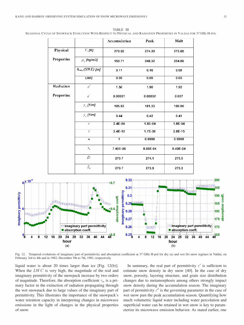
The yellow square, triangle, and circle markers in Fig. 11identify times corresponding to different phases of snowpackevolution, respectively, accumulation, peak, and melting at18:00 LST for an arbitrary day in Valdai. Table III shows andcompares snow hydrology and microwave emission parametersat each of the three times in the snowpack evolution. The SWEdecreases after the accumulation season peak due to loss ofsnowpack mass as a result of intermittent melting episodes,whereas the density ρs monotonically increases up to the onset

of the runaway melting phase proper. Although the temporalevolution of brightness temperatures follows closely the evolu-tion of snowpack temperature Ts, discrepancies are expected assnow density changes. The most important attenuation factorin the wet snow regime is the absorption of radiation per unitlength of the line of wave propagation, and thus the key radio-metric property contributing to the decrease of the brightnesstemperature is the absorption coefficient γa. Consequently, theinterface reflectivity s1 increases by two orders of magnitudeduring the accumulation phase due to the increase in the realpart of the permittivity. This explains the difference betweenthe physical snow temperature and the brightness temperatures:the outgoing radiation from the snowpack decreases due toincreasing interface reflectivity s1 of the snowpack at the peakof the snow accumulation season, and increases with D1 [(15),Section II-B]. Because melting processes involve both mass andenergy transfer, the evolution of an internal bulk property suchas density ρs can be viewed as a proxy of the joint evolution ofthe internal energy and structure of the snowpack that integratesinformation state variables such as Ts and SWE as pointedout earlier by [27] regarding the relationship between snowpermittivity and density [27]. In turn, the radiometric propertiescan be viewed as diagnostics of snow wetness, and ultimatelySWE. This is further addressed next.

C. Diurnal Cycle of Snow Microwave Emissions

To assess the diurnal cycle of the snowpack microwave emis-sion, two cases are examined for dry and wet snow snowpackregimes and for 37 GHz V-pol, which is sensitive to scatteringas a function of snow grain size, and has been widely used in theretrieval of snow physical properties from remote sensing data(e.g. [17]). The dry snow case is from February 3rd to 4th in1982 corresponding to the time marked by the green rhombusin Fig. 11. Note that the overall LWC values are negligibleduring the 48 h of simulation from midnight on February 2nd tomidnight on February 4th. The wet snow case is from midnighton December 5th to midnight on December 7th in 1981, andcorresponds to the time marked by the green parallelogram inFig. 11. The LWC is always above 4% during this period.Fig. 12(a) and (b) shows time series of radiation parameters,imaginary permittivity, and absorption coefficient comparedwith snow density both for dry and wet snow. Although theabsorption coefficient strongly varies with the imaginary partof the permittivity both in dry and wet cases, the magnitudeof the absorption coefficient for wet snow is three orders ofmagnitude that for dry snow. This significant increase in theabsorption coefficient contributes to the simulated changes inthe attenuation behavior of the wet snow. In MEMLS, theabsorption coefficient γa is a function of the refractive indexn′′ [γa = 4πn′′/λ, (17)], and n′′ is a function of the real andimaginary permittivity

n′′ =sgn(ε′′)√

2

√√ε′2 + ε′′2 − ε′. (27)

The imaginary part of permittivity can significantly increasewith increasing LWC because the imaginary part of volumetric


TABLE IIISEASONAL CYCLE OF SNOWPACK EVOLUTION WITH RESPECT TO PHYSICAL AND RADIATION PROPERTIES IN VALDAI FOR 37 GHz H-POL

Fig. 12. Temporal evolutions of imaginary part of permittivity and absorption coefficient at 37 GHz H-pol for dry (a) and wet (b) snow regimes in Valdai, onFebruary 3rd to 4th and in 1982, December 5th to 7th, 1981, respectively.

liquid water is about 20 times larger than ice [Fig. 12(b)].When the LWC is very high, the magnitude of the real andimaginary permittivity of the snowpack increase by two ordersof magnitude. Therefore, the absorption coefficient γa is a pri-mary factor in the extinction of radiation propagating throughthe wet snowpack due to large values of the imaginary part ofpermittivity. This illustrates the importance of the snowpack’swater retention capacity in interpreting changes in microwaveemissions in the light of changes in the physical propertiesof snow.

In summary, the real part of permittivity ε′ is sufficient toestimate snow density in dry snow [40]. In the case of drysnow, porosity, layering structure, and grain size distributionchanges due to metamorphosis among others strongly impactsnow density during the accumulation season. The imaginarypart of permittivity ε′′ is the governing parameter in the case ofwet snow past the peak accumulation season. Quantifying howmuch volumetric liquid water including water percolation andsuperficial water can be retained in wet snow is key to param-eterize its microwave emission behavior. As stated earlier, one


Fig. 13. Snow temperature simulation compared with composite from various snow pit measurements in February and March 2003 from the three ISAs (Fig. 2)located within the Fraser MSA for CLPX.

interesting implication of this behavior is that instead of usingphysical properties to describe snowpack conditions, radiationproperties such as permittivity, and absorption and scatteringcoefficients can be viewed as alternative state variables todescribe snowpack conditions.

V. RESULTS AND DISCUSSION—CLPX

The focus here is on the application of MLSHM to theFraser MSA during CLPX (Fig. 2). Results of the LSHMsnow hydrology forced by RUC40 (40 km resolution) werediscussed briefly in Section III-E. Fig. 13(a) and (b) showsthe simulated snowpack physical temperature Ts comparedwith snow pit profile observations during February and March,2003 within the Fraser, MSA. Multiple points for each daterepresent measurements at various sampling depths for eachsnow pit. The LSHM single layer snowpack temperature Ts isaround the mean value of the observed snow pit temperatures,particularly in the afternoon. Fig. 14 shows the simulatedbrightness temperatures Tb using RUC40 forcing (40× 40 km2

pixel area) compared against SSM/I EASE products with25× 25 km2 spatial resolution at their respective frequenciesand polarizations from October 2002 to June 2003. Table IVincludes AMSR-E comparison statistics as well as SSM/I. Notethat although both SSM/I and AMSR-E EASE-grid productsprovide ToA brightness temperatures, in this case, no correctionwas made because at the continental high altitudes of CLPX,the atmosphere is very dry (precipitable water during the coldseason is less than 5 mm on average, and thus the impact ofthe correction is negligible—not shown), and because therewas not a long enough record to calibrate locally meaningfulcoefficients for (25). In addition, no such correction was ap-plied in previous studies used here as baseline target for theperformance of the MLSHM in prognostic OSS mode.

The simulations in Fig. 14 indicate that MLSHM-SL Tbsmatch generally well the observations particularly during themelting phase. In winter, during the accumulation phase, thereis some bias particularly at 37 GHz V-pol similar to resultsreported earlier by [41], but more importantly, the model is not

capturing the concave shape exhibited by SSM/I observationsconsistent with increasingly colder brightness temperatures andincreasing snow density (Fig. 14). The behavior is similar forAMSR-E (not shown). Inspection of Fig. 6 indicates that themodel underestimates snow density which can explain thisbehavior at least in part and should be particularly critical forvertical polarization [37]. In addition to changes in density,increases in snow grain size as the snowpack ages due tometamorphic processes such as depth hoar, which are notexplicitly described in the model, lead to increasing volumescattering and increasingly cold temperatures. [42] found thatthis effect was particularly important at 37 GHz V-pol usingthe SL HUT model, not unlike the results presented here.Moreover, the presence of trees, which can be an importantmicrowave signal in some areas in CLPX [5], [22], is notexplicitly described in MEMLS, and in the LSHM, the effectis only accounted for in terms of fractional vegetation covereffects on the surface energy balance, but not in terms of itsimpact on snow properties (see Section II). Nevertheless, bythe end of March and through the snowpack warming phase tillMay, there is good agreement between simulated and observedbrightness temperatures even at 37 GHz.

Previously, [23] and [24] focused on modeling the emissionbehavior of a dry snow regime during CLPX, February 19–24,2003 at the GBMR-7 location. [24] simulated AMSR-E obser-vations for the entire month of February using the variable in-filtration capacity (VIC) hydrology model coupled with DMRTto simulate the bulk layer snowpack including snow density,snow temperature, SD, and snow grain size, and comparedtheir model results against one week (February 18–26, 2003)of observations at GBMR-7 during dry snow conditions. Theypresent results of VIC simulations from 1 October 2002 throughthe late accumulation season on March 28, 2003. Their resultsare in line with LSHM results presented in Fig. 6. [23] importedobserved snow pit stratigraphy and measured snow propertiesat GBMR-7 directly into MEMLS. [25] used a version of theHUT model as well as DMRT and MEMLS coupled to VICfor simulations at two sites within the Fraser MSA February–May 2003, thus including both dry and wet snow regimes


Fig. 14. Intercomparison among observed SSM/I (blue square) and LSHM-MEMLS (red circle) simulations at 37 (top panels), 22.2 (midpanels), and19.35 (bottom panels) GHz H-pol and V-pol. Observations at 22 GHz, H-pol are not available.

over a four-month period. Summary microwave emission errorstatistics for the entire period of simulation from October2002 through June 2003 are summarized in Table IV usingthe same measures described in Section IV-A. Although theMLSHM predictions spanned the October–June period, be-cause the range of conditions encompassed by [25] is morecomprehensive and representative of the intermittency of snow-pack regimes over an entire season than other references,Table IV also includes error statistics reported by [25] withrespect to AMSR-E.

Overall, the MEMLS’ simulations using LSHM snowpackphysical properties show errors statistics similar or better thanprevious studies for all three channels in H and V pol. TheMLSHM-SL performance is particularly noteworthy for ME at36.5 GHz H-pol (8.5 K in this study versus 11.2 K in [23]).An application with similar results was conducted by [22] atGBMR-7 using DMRT instead of MEMLS. Thus, despite thespatial scale disparities and the differences in ancillary dataavailability, duration of simulations (days versus snow seasonin this study), and different snow regimes (both wet and dry,

accumulation and melting phases in this study), the error statis-tics of end-to-end MLSHM brightness temperatures are in linewith previous studies, and significantly improved at 37 GHzH-pol. Table IV suggests that the bulk microwave emissionerror statistics against AMSR-E are significantly better thanagainst SSM/I at 18–19 GHz V-pol, but the reverse is true for37 GHz H-pol. Inspection of the actual time series indicates,however, that overall qualitative behavior is better captured forAMSR-E, and therefore improved bulk error statistics may bein part the artifact of error cancelation effects.

Large abrupt changes in emissivity behavior, and thus bright-ness temperatures, between wet and dry snow regimes can belinked to changes in snow volumetric LWC. Fig. 15 shows therelationship between snow density and two simulated radio-metric variables, respectively, the snowpack bulk reflectivity[Fig. 15(a)] and the snowpack–atmosphere interface reflectivity[Fig. 15(b)] for 37 GHz H-pol. Fig. 15(a) shows an inverserelationship between snow density and the bulk reflectivity. Asreviewed earlier, because the snow density is directly relatedto the complex permittivity, the density is therefore directly


TABLE IVERROR STATISTICS OF BRIGHTNESS TEMPERATURES Tsim SIMULATED BY MLSHM-SL FORCED BY RUC40 FOR CLPX (FRASER-MSA) FOR BOTH SSM/I

AND AMSR-E OCTOBER 2002–JUNE 2003, AND STATISTICS FOR AMSR-E FROM [25]. NOTE: 22 GHz H-POL FROM SSM/I IS NOT AVAILABLE.AMSR-E (SSM/I) FREQUENCIES ARE 18.7 (19.35) GHz, 23.8 (22.2) GHz, AND 36.5 (37) GHz

Fig. 15. Annual behavior of bulk reflectivity of the snowpack (a) and surface reflectivity sn (b) along with snow density, both at 37 GHz H-pol and at theGBMR-7 location using atmospheric forcing from the GBMR-7 tower instead of RUC40 forcing.


Fig. 16. Increase of brightness temperature induced by snow wetness at37 GHz V-pol SSM/I (blue filled circle), Tapp (red star), and rainfall (blacksolid line) during February, 2003 for CLPX using meteorological data from thetower at the GBMR-7 location instead of RUC40 forcing.

related to the snowpack surface reflectivity and bulk reflec-tivity. During the accumulation phase, the internal reflectivitydecreases with increasing snow density when the snowpackis deeper than for shallow snowpacks early in the season. Onthe other hand, Fig. 15(b) shows that the interface reflectivityis proportional to the snow density. This is because the snowdensity directly influences the real part of the permittivity.Generally, there is therefore a strong relationship between bulksnow physical attributes and radiometric characteristics such asreflectivity, transmissivity, emissivity, and interface reflectivity,which lends support to the parameterization of snow correlationlength in terms of snow density [28]. Conversely, changes inradiometric behavior can be linked to changes in snowpackphysical properties, which suggests a path for monitoring snow-pack physical properties from space. Note that the results inFig. 15 were obtained by running the MLSHM-SL with forcingobtained from the GBMR-7 site, in contrast with the results inFig. 6 using RUC-40 forcing. The simulated density past theend of March in Fig. 15 is significantly improved as comparedto the results using RUC-40 forcing in Fig. 6, though thereis a slight increase in the Bias during the accumulation sea-son. That is, the GBMR-7 tower registers rainfall that RUC40forecasts missed. These results show the importance of small-scale spatial heterogeneities, and in particular increases of snowwetness due to rain-on-snow effects on snowpack radiometricproperties, and consequently on passive microwave emission.

To further illustrate this point, simulated (MLSHM) andobserved (SSM/I) Tbs at 37 GHz V-pol using the GBMR-7forcing are shown in Fig. 16. Note how rainfall causes a short-duration increase in simulated brightness temperatures due tothe transient increase of LWC in the snowpack, as well assubsequent warming due to latent heating release as the rainwa-ter freezes. As expected, the microwave emission simulationswith GBMR-7 meteorological data to force the model duringthis February simulation are closer to the observations thanthe microwave emission simulations with RUC40 (Fig. 14 toppanels), in part due to the ability to capture local variationsof the volumetric LWC due to rainfall. Overall, however, atthe scale of the Fraser MSA, the MLSHM simulation usingRUC40 is more reliable to simulate the entire 2002–2003 water

year of 2002 than the local scale observations at the GBMR-7meteorological measurement data.

VI. SUMMARY AND DISCUSSION

A coupled snow hydrology-microwave emission modelMLSHM [1]–[3] was evaluated in OSS mode against space-borne microwave observations from SMMR, SSM/I, andAMSR-E in two very different climatic and physiographicregions (Valdai and Colorado, CLPX) for both wet and drysnow regimes over multiple years with good results. These ap-plications demonstrate robustness of the modeling system andits potential utility in large-scale snow monitoring over largeareas with limited if any ground-based observations to constrainthe model or for data assimilation. Despite overall good skillas demonstrated by relatively low errors, one weakness wasidentified with respect to the simulation of the microwaveemission behavior of the snowpack, particularly for horizontalpolarization, when ice layers (ice lenses, ice fingers [20]) formdue to freezing of volumetric liquid water either due to daytimemelting or due to rain-on-snow events. Another likely source oferror is the lack of representation of snow interception by vege-tation, the representation of the radiometric signature of snow-covered trees, as well as the characteristics of the snowpackunder vegetation [51], [62]. In addition, subgrid-scale land-useand other land-cover heterogeneities [52] cannot be explicitlyrepresented in the model at the RUC40 spatial resolution. Giventhe importance of snow density and volumetric LWC, a moreaccurate estimation of snow density, particularly in the caseof wet snow regimes, is necessary to improve the results forvertical polarization.

One approach to address these weaknesses is to implementthe ML snow hydrology model to capture heterogeneities inthe vertical structure of the snowpack due to rain-on-snow andmelting events, and to capture snowpack gradients in temper-ature and water content that change its microwave emissionbehavior. Furthermore, a ML representation of the snowpackallows taking advantage of the ML structure in MEMLS. Re-search toward evaluating the parameterization of snow micro-physical processes specifically regarding the temporal evolutionof the vertical distribution of grain size distribution, presentlydescribed in terms of an empirical relationship between snowdensity and correlation length pec is also necessary. The cor-relation length is a governing parameter in the estimationof the scattering coefficient γb and of the surface roughnessof the snowpack, and the bulk representation adopted in thecurrent MLSHM-SL is insufficient to capture the effects ofheterogeneities, gravitational settling, and metamorphic pro-cesses [38]. These conclusions are consistent with the resultsof a study comparing radiative transfer models for passivemicrowave remote sensing of snow performed by [41] usingboth sensitivity analysis and evaluation of simulated brightnesstemperatures against experimental observations using ground-based observations of snowpack properties. [41] stressed theimportance of the relationship between mean grain size and cor-relation length as a function of snowpack conditions and history(e.g. density and grain size growth with snow age), and the rep-resentation of multiple layers. The latter is addressed in Part 2


[56]. The contribution of the fractional vegetation cover gener-ally, and forests in particular, to the radiometric signature of thelandscape is a difficult problem that cannot be ignored. Whereasland-cover sensitive empirical algorithms have been developed[64], significant place-based calibration is required. This is anarea whether combined active-passive emission models, andconversely retrieval models, may present a significant advan-tage, as there are parameterizations of vegetation backscatterthat are well understood [36], [54]. Significant improvementswith locally calibrated atmospheric correction parameters inValdai suggest there is an opportunity to further investigatethe effectiveness of atmospheric correction algorithms currentlyused in operational retrievals toward developing place-basedoptimal parameterizations making use of global data sets suchas ERA40 for example.

Finally, the two applications of the MLSHM-SL confirm ourhypothesis that, despite its simplicity, the SL formulation is arobust strategy to predict SD and SWE over remote regions us-ing numerical weather prediction forecasts as forcing in regionswhere satellite remote sensing provides the only observationsto evaluate operational monitoring effectiveness of snowpackcondition and water resources.

ACKNOWLEDGMENT

We are thankful to the Reviewers and Editors for theircomments and suggestions.

REFERENCES

[1] E. Devonec and A. P. Barros, “Exploring the transferability of a land-surface hydrology model,” J. Hydrol., vol. 265, no. 1–4, pp. 258–282,Aug. 2002.

[2] A. Wiesmann and C. Mätzler, “Microwave emission model of lay-ered snowpacks,” Remote Sens. Environ., vol. 70, no. 3, pp. 307–316,Dec. 1999.

[3] C. Mätzler and A. Wiesmann, “Extension of the microwave emissionmodel of layered snowpacks to coarse grained snow,” Remote Sens.Environ., vol. 70, no. 3, pp. 317–325, Dec. 1999.

[4] C. Derksen and A. E. Walker, “Identification of systematic bias in thecross-platform (SMMR and SSM/I) EASE-grid brightness temperaturetime series,” IEEE Trans. Geosci. Remote Sens., vol. 41, no. 4, pp. 910–915, Apr. 2003.

[5] D. Cline, K. Elder, B. Davis, J. Hardy, G. E. Liston, D. Imel, S. H. Yueh,A. J. Gasiewski, G. Koh, R. L. Armstrong, and M. Parsons, “Overview ofthe NASA cold land processes field experiment,” in Proc. SPIE—Int. Soc.Opt. Eng., 2003, vol. 4894, pp. 361–372.

[6] National Research Council, “Earth Science and Applications from Space:National Imperatives for the Next Decade and Beyond,” Washington, DC:Nat. Academic Press, 2007.

[7] J. W. Pomeroy and D. M. Gray, “Snow accumulation, relocation andmanagement,” Nat. Hydrology Res. Inst. Sci., Burlington, ON, Canada,Report 7144, 1995.

[8] A. Lundberg, “Laboratory calibration of TDR-probes for snow wetnessmeasurements,” Cold Regions Sci. Technol., vol. 25, no. 3, pp. 197–205,Apr. 1997.

[9] N. Granlund, A. Lundbert, J. Feiccabrino, and D. Gustafsson, “Laboratorytest of snow wetness influence on electrical conductivity measured withground penetrating radar,” Hydrol. Res., vol. 40, no. 1, pp. 33–44, 2009.

[10] A. Lundberg, H. Thunehed, and J. Bergström, “Impulse radarsnow surveys—Influence of snow density,” Nordic Hydrol., vol. 31, no. 1,pp. 1–14, 2000.

[11] A. Lundberg and H. Thunehed, “Snow wetness influence on impulse radarsnow surveys theoretical and laboratory study,” Nordic Hydrol., vol. 31,no. 2, pp. 89–106, 2000.

[12] D. Kang and A. Barros, “Introducing an L-band snow sensor system forin situ monitoring of changes in water content-full system testing,” IEEETrans. Geosci. Remote Sens., vol. 49, no. 3, pp. 908–919, 2011.

[13] J. L. Foster, A. T. C. Chang, and D. K. Hall, “Comparison of snowmass estimates from a prototype passive microwave algorithm and a snowdepth climatology,” Remote Sens. Environ., vol. 62, no. 2, pp. 132–142,Nov. 1997.

[14] R. L. Armstrong and M. J. Brodzik, “Recent northern hemisphere snowextent: A comparison of data derived from visible and microwave satellitesensors,” Geophys. Res. Lett., vol. 28, no. 19, pp. 3673–3676, 2001.

[15] R. Kelly, A. Chang, L. Tsang, and J. Foster, “A prototype AMSR-E globalsnow area and snow depth algorithm,” IEEE Trans. Geosci. Remote Sens.,vol. 41, no. 2, pp. 230–242, Feb. 2003.

[16] T. Markus, D. J. Cavalieri, A. J. Gasiewski, M. Klein, J. A. Maslanik,D. C. Powell, B. B. Stankov, J. C. Stroeve, and M. Sturm, “Microwavesignatures of snow on sea ice: Observations,” IEEE Trans. Geosci. RemoteSens., vol. 44, no. 11, pp. 3081–3090, Nov. 2006.

[17] A. T. C. Chang, J. L. Foster, and D. K. Hall, “Nimbus-7 derived globalsnow cover parameters,” Ann. Glaciol., vol. 9, no. 9, pp. 39–44, 1987.

[18] C. Kummerow, Y. Hong, W. S. Olson, S. Yang, R. F. Adler, J. McCollum,R. Ferraro, G. Petty, D.-B. Shin, and T. T. Wilheit, “The evolution of theGoddard profiling algorithm (GPROF) for rainfall estimation from passivemicrowave sensors,” J. Appl. Meteorol., vol. 40, no. 11, pp. 1801–1820,Nov. 2001.

[19] J. Pulliainen, J. Grandell, and M. T. Hallikainen, “HUT snow emissionmodel and its applicability to snow water equivalent retrieval,” IEEETrans. Geosci. Remote Sens., vol. 37, no. 3, pp. 1378–1390, May 1999.

[20] J. Lemmetyinen, J. I. Pulliainen, J. Rees, A. Kontu, and Y. Qiu, “Multiple-layer adaptation of HUT snow emission model: Comparison with experi-mental data,” IEEE Trans. Geosci. Remote Sens., vol. 48, no. 7, pp. 2781–2794, Jul. 2010.

[21] L. Tsang, C. Chen, A. T. C. Chang, J. Guo, and K. Ding, “Dense mediaradiative transfer theory based on quasicrystalline approximation withapplications to passive microwave remote sensing of snow,” Radio Sci.,vol. 35, no. 3, pp. 731–749, 2000.

[22] M. Tedesco, E. J. Kim, D. Cline, T. Graf, T. Koike, R. Armstrong,M. Brodzik, B. Stankov, A. Gasiewski, and M. Klien, “Exploring scal-ing issues by using NASA cold processes experiment (CLPX-1, IOP3)radiometric data,” in Proc. IEEE Int. Geosci. Remote Sens., Anchorage,AK, 2004, pp. 1657–1660.

[23] M. Durand, E. J. Kim, and S. A. Margulis, “Quantifying uncertaintyin modeling snow microwave radiance for a mountain snowpack at thepoint-scale, including stratigraphic effects,” IEEE Geosci. Remote Sens.,vol. 46, no. 6, pp. 1753–1767, Jun. 2008.

[24] K. M. Andreadis, D. Liang, L. Tsang, and D. P. Letenmaier, “Charac-terization of errors in a coupled snow hydrology-microwave emissionmodel,” J. Hydrometeorol., vol. 9, no. 1, pp. 149–164, 2008.

[25] R. Wójcik, K. Andreadis, M. Tedesco, E. Wood, T. Troy, andD. Lettenmeier, “Multimodel estimation of snow microwave emissionduring CLPX 2003 using operational parameterization of microphysicalsnow characteristics,” J. Hydrometeorol., vol. 9, no. 6, pp. 1491–1505,Mar. 2008.

[26] R. Jordan, “A one-dimensional temperature model for a snow cover,” U.S.Army Corps of Engineers, Washington, DC, Special Rep. 91-16, 1991.

[27] A. Wiesmann and C. Mätzler, “Radiometric and structural measurementsof snow samples,” Radio Sci., vol. 33, no. 2, pp. 273–290, 1998.

[28] C. Mätzler, “Relation between grain-size and correlation length of snow,”J. Glaciol., vol. 48, no. 162, pp. 461–466, Jun. 2002.

[29] J. Aschbacher, “Parameterization of atmospheric influence for microwaveland surface radiometry,” in Proc. Int. Geosci. Remote Sens. Symp., 1990,vol. 2, pp. 1551–1554.

[30] B. J. Choudhury, “Atmospheric effects on SMMR and SSM/I 37 GHzpolarization difference over the Sahel,” Int. J. Remote Sens., vol. 13,no. 18, pp. 3443–3463, 1992.

[31] E. R. Westwater, J. B. Snider, and M. J. Falls, “Ground-based radiometricobservations of atmospheric emission and attenuation at 20.3, 31.65, and90.0 GHz: A comparison of measurements and theory,” IEEE Trans.Antennas Propag., vol. 38, no. 10, pp. 1569–1580, Oct. 1990.

[32] C. Mätzler, “Ground-based observations of atmospheric radiation at 5,10, 21, 35, and 94 GHz,” Radio Sci., vol. 27, no. 3, pp. 403–415,May/Jun. 1992.

[33] P. Gloersen and F. T. Barath, “A scanning multichannel microwave ra-diometer for Nimbus-G and SeaSat-A,” IEEE J. Ocean. Eng., vol. OE-2,no. 2, pp. 172–178, Apr. 1977.

[34] A. Henderson-Sellers, Z. L. Yang, and R. E. Dickinson, “The project forintercomparison of land-surface parameterization schemes,” Bull. Amer.Meteorol. Soc., vol. 74, no. 7, pp. 1335–1350, Jul. 1993.

[35] S. M. Uppala, P. W. Kallberg, A. J. Simmons, U. Andrae, V. Da CostaBechtold, M. Fiorino, J. K. Gibson, J. Haseler, A. Hernandez, G. A. Kelly,X. Li, K. Onogi, S. Saarinen, N. Sokka, R. P. Allan, E. Andersson,


K. Arpe, M. A. Balmaseda, A. C. M. Beliaars, L. Van De Berg, J. Bidlot,N. Bormann, S. Caires, F. Chevallier, A. Dethof, M. Dragosavac,M. Fuentes, S. Hagenmann, E. Holm, B. J. Hoskins, L. Isaksen,P. A. E. M. Janssen, R. Jenne, A. P. McNally, E. Holm, B. J. Hoskins,L. Isaksen, P. A. E. M. Janssen, R. Jenne, A. P. McNally, J. F. Mahfouf,J. J. Morcrette, N. A. Ravner, R. W. Saunders, P. Simon, A. Sterl,K. E. Trenberth, A. Untch, D. Vasilievic, P. Viterbo, and J. Woolen, “TheERA-40 re-analysis,” Quart. J. Roy. Meteorol. Soc., vol. 131, no. 612,pp. 2961–3012, Oct. 2005.

[36] A. N. Arslan, J. Koskinen, J. Pulliainen, and M. Hallikainen, “A semiempirical backscattering model of forest canopy covered by snow usingSAR data,” in Proc. IGARSS, Honolulu, HI, 2000, vol. 5, pp. 1904–1906.

[37] A. Rees, J. Lemmetyinen, C. Derksen, J. Pulliainen, and M. English, “Ob-served and modelled effects of ice lens formation on passive microwavebrightness temperatures over snow covered tundra,” Remote Sens.Environ., vol. 114, no. 1, pp. 116–126, Jan. 2010.

[38] V. Roy, K. Goita, A. Royer, A. E. Walker, and B. E. Goodison, “Snowwater equivalent retrieval in a Canadian boreal environment,” IEEE Gosci.Remote Sens., vol. 42, no. 9, pp. 1850–1859, Sep. 2004.

[39] C. A. Schlosser, A. G. Slater, A. Robock, A. J. Pitman, K. Y. Vinnikov,A. Henderson-Sellers, N. A. Speranskaya, K. Mitchell, A. Boone,H. Braden, F. Chen, P. Cox, P. de Rosnay, C. Desborough, andR. E. Dickenson, “Simulations of a boreal grassland hydrology at Valdai,Russia:PILPS phase 2(d),” Monthly Weather Rev., vol. 128, no. 2, pp. 301–321, Feb. 2000.

[40] W. A. Cumming, “The dielectric properties of ice and snow at 3.2 cen-timeters,” J. Appl. Phys., vol. 23, no. 7, pp. 768–773, Jul. 1952.

[41] M. Tedesco and E. J. Kim, “Intercomparison of Electromagnetic Modelsfor Passive Microwave Remote Sensing of Snow,” IEEE Trans. Geosci.Remote Sens., vol. 44, no. 10, pp. 2654–2666, Oct. 2006.

[42] M. J. Butt and R. E. J. Kelly, “Estimation of snow depth in the UK usingthe HUT snow emission model,” Int. J. Remote Sens., vol. 29, no. 14,pp. 4249–4267, Jul. 2008.

[43] K. W. Knowles, E. Njoku, R. L. Armstrong, and M. J. Brodzik, Nimbus-7SMMR Pathfinder Daily EASE-Grid Brightness Temperatures. Boulder,CO: Nat. Snow and Ice Data Center Media, 2002.

[44] E. A. Anderson, “Development and testing of snow pack energy balanceequations,” Water Resour. Res., vol. 4, no. 1, pp. 19–37, 1968.

[45] D. Marks and J. Dozier, “A clear-sky longwave radiation model for re-mote alpine areas,” Arch. Meteorol. Geophys. Bioclimatol. Ser. B, vol. 27,no. 2/3, pp. 159–187, Jun. 1979.

[46] E. M. Morris, “Sensitivity of the European hydrological system snowmodels,” in Proc. Exeter Symp. IAHS, 1982, vol. 138, pp. 221–231.

[47] G. N. Flerchinger and K. E. Saxton, “Simultaneous heat and water modelof a freezing 26 snow-residue-soil system 1. Theory and development,”Trans. ASAE, vol. 32, no. 2, pp. 565–571, 1989.

[48] G. Bloschl, R. Kirnbauer, and D. Gutknecht, “Distributed snowmelt sim-ulations in an alpine catchment, 1, Model evaluation on the basis of snowcover patterns,” Water Resour. Res., vol. 27, no. 12, pp. 3171–3179, 1991.

[49] R. G. Barry, Mountain Weather and Climate, 2nd ed. London, U.K.:Routledege Phys. Environ. Series, 1992, 402 pp.

[50] F. Zanotti, S. Endrizzi, G. Bertoldi, and R. Rigon, “The GEOTOPsnow module,” Hydrological Process., vol. 18, no. 18, pp. 3667–3679,Dec. 2004.

[51] Y. Kim, J. S. Kimball, K. C. McDonald, and J. Glassy, “Developing aglobal data record of daily landscape freeze/thaw status using satellitepassive microwave remote sensing,” IEEE Trans. Geosci. Remote Sens.,vol. 49, no. 3, pp. 949–960, Mar. 2011.

[52] N. Pierdiccas, L. Pulvirenti, and F. S. Marzano, “Simulating topographiceffects on spaceborne radiometric observations between L and X fre-quency bands,” IEEE Trans. Geosci. Remote Sens., vol. 48, no. 1, pp. 273–282, Jan. 2010.

[53] O. T. Farouki, Thermal Properties of Soils. Hanover, NH: USA ColdRegions Res. Eng. Lab., 1981, CRREL Monograph 81-1.

[54] R. Bindlish and A. P. Barros, “Parameterization of Vegetation Backscatterin radar- based soil moisture estimation,” Remote Sens. Environ., vol. 76,no. 1, pp. 130–137, Apr. 2001.

[55] S. Frankenstein, A. Sawyer, and J. Koeberle, “Comparison of FASSTand SNTHERM in three snow accumulation regimes,” J. Hydrometeorol.,vol. 9, no. 6, pp. 1443–1463, Dec. 2008.

[56] D.-H. Kang and A. P. Barros, “Observing system simulation of snow mi-crowave emissions over data sparse regions. Part 2: Multi-layer physics,”IEEE Trans. Geosci. Remote Sens., 2011, to be published.

[57] T. Markus, D. C. Powell, and J. R. Wang, “Sensitivity of passive mi-crowave snow depth retrievals to weather effects and snow evolution,”IEEE Trans. Geosci. Remote Sens., vol. 44, no. 1, pp. 68–77, Jan. 2006.

[58] M. Tedesco and J. R. Wang, “Atmospheric correction of AMSR-E bright-ness temperatures for dry snow cover mapping,” IEEE Trans. Geosci.Remote Sens. Lett., vol. 3, no. 3, pp. 320–324, Jul. 2006.

[59] J. R. Wang and M. Tedesco, “Identification of atmospheric influences onthe estimation of snow water equivalent from AMSR-E measurements,”Remote Sens. Envriron., vol. 111, no. 2/3, pp. 398–408, Nov. 2007.

[60] M. J. Brodzik, R. Armstrong, and M. Savoie, Global EASE-Grid 8-dayBlended SSM/I and MODIS Snow Cover. Boulder, CO: Nat. Snow andIce Data Center. Digital Media, 2007.

[61] M. Tedesco, R. E. J. Kelly, J. L. Foster, and A. T. L. Chang, AMSR-E/AquaDaily L3 Global Snow Water Equivalent EASE-Grids V002. Boulder,CO: Nat. Snow and Ice Data Center. Digital media, 2004, updated daily.

[62] C. Derksen, A. Walker, and B. Goodison, “A comparison of 18 winterseasons of in situ and passive microwave-derived snow water equivalentestimates in Western Canada,” Remote Sens. Environ., vol. 88, no. 3,pp. 271–282, Dec. 2003.

[63] A. Langlois, A. Royer, and K. Gota, “Analysis of simulated and space-borne passive microwave brightness temperatures using in situ measure-ments of snow and vegetation properties,” Can. J. Remote Sens., vol. 36,no. Suppl. 1, pp. S135–S148, 2010.

[64] C. Derksen, P. Toose, A. Rees, L. Wang, M. English, A. Walker, andM. Sturm, “Development of a tundra-specific snow water equivalentretrieval algorithm for satellite passive microwave data,” Remote Sens.Environ., vol. 114, no. 8, pp. 1699–1709, Aug. 2010.

Do Hyuk Kang received the B.A. degree in geog-raphy from Seoul National University, Seoul, Korea,the M.S. degree in civil engineering from ColoradoState University, Fort Collins, and the Ph.D. degreein civil engineering from Duke University, Durham,NC, in December 2010.

His research interests include the applications ofL band sensors to measure geophysical layers anda hydrology model coupled with forward models ofpassive and active microwave remote sensing.

Ana P. Barros (M’94–SM’04) received the diplomain civil engineering with majors in structures and hy-draulics and the M.Sc. degree in ocean engineeringfrom the Faculty of Engineering, University of Porto,Porto, Portugal, the M.Sc. degree in environmentalscience and engineering from the Oregon Gradu-ate Institute, Oregon Health and Science University,Portland, and the Ph.D. degree in civil engineeringfrom the University of Washington, Seattle, in 1985,1988, 1990, and 1993, respectively.

She was a Faculty Member with The PennsylvaniaState University, University Park, and with Harvard University, Cambridge,MA. She is currently a Professor of engineering with Duke University,Durham, NC.

ieee transactions on geoscience and …web.unbc.ca/~dkang/index_files/tgrs-kang-2169073-x.pdfyear...

Documents