ieee transactions on software …das.encs.concordia.ca/uploads/2016/01/kamei_tse2013.pdfa...

A Large-Scale Empirical Study ofJust-in-Time Quality Assurance

Yasutaka Kamei, Member, IEEE, Emad Shihab, Bram Adams, Member, IEEE,

Ahmed E. Hassan, Member, IEEE, Audris Mockus, Member, IEEE, Anand Sinha, and

Naoyasu Ubayashi, Member, IEEE

Abstract—Defect prediction models are a well-known technique for identifying defect-prone files or packages such that practitioners

can allocate their quality assurance efforts (e.g., testing and code reviews). However, once the critical files or packages have been

identified, developers still need to spend considerable time drilling down to the functions or even code snippets that should be reviewed

or tested. This makes the approach too time consuming and impractical for large software systems. Instead, we consider defect

prediction models that focus on identifying defect-prone (“risky”) software changes instead of files or packages. We refer to this type of

quality assurance activity as “Just-In-Time Quality Assurance,” because developers can review and test these risky changes while they

are still fresh in their minds (i.e., at check-in time). To build a change risk model, we use a wide range of factors based on the

characteristics of a software change, such as the number of added lines, and developer experience. A large-scale study of six open

source and five commercial projects from multiple domains shows that our models can predict whether or not a change will lead to a

defect with an average accuracy of 68 percent and an average recall of 64 percent. Furthermore, when considering the effort needed to

review changes, we find that using only 20 percent of the effort it would take to inspect all changes, we can identify 35 percent of all

defect-inducing changes. Our findings indicate that “Just-In-Time Quality Assurance” may provide an effort-reducing way to focus on

the most risky changes and thus reduce the costs of developing high-quality software.

Index Terms—Maintenance, software metrics, mining software repositories, defect prediction, just-in-time prediction

Ç

1 INTRODUCTION

SOFTWARE quality assurance activities (e.g., source codeinspection and unit testing) play an important role in

producing high quality software. Software defects1 inreleased products have expensive consequences for acompany and can affect its reputation. At the same time,companies need to make a profit, so they should minimizethe cost of maintenance activities. To address this challenge,a plethora of software engineering research focuses onprioritizing software quality assurance activities [4], [6], [49].

The majority of quality assurance research is focused ondefect prediction models that identify defect-prone mod-ules (i.e., files or packages) [17], [19], [30], [45]. Althoughsuch models can be useful in some contexts, they also havetheir drawbacks. We can summarize the drawbacks of suchapproaches as follows:

1. Prediction units are coarse grained: Predictions atthe package or file granularity leave it to developersto locate the risky code snippets in these files.

2. Relevant experts are not identified: Once a file isidentified as risky, someone needs to find the expertfor inspection/testing and other quality improve-ment activities. This may be a nontrivial task: Forexample, some files in the Mozilla project aretouched by up to 155 developers.

3. Predictions are made too late in the developmentcycle: Practitioners want to know about qualityissues as soon as possible while the change detailsare still fresh in their minds.

Therefore, researchers have proposed performing pre-dictions at the change level, focusing on predicting defect-inducing changes [26], [41]. We illustrate the advantage ofchange-level prediction with the following example: Alice isa software development manager for a large legacy systemthat is subject to on-going maintenance. Bob and Chris aretwo developers of the system, and Bob has modified a file A.A year later, in the course of estimating the expected qualityof the upcoming release, a package/file-level predictionmodel used by Alice indicates that file A is fault prone.Given the length of time that has passed since the change,Alice does not know who’s change introduced the defect.

IEEE TRANSACTIONS ON SOFTWARE ENGINEERING, VOL. 39, NO. 6, JUNE 2013 757

. Y. Kamei and N. Ubayashi are with the Graduate School and Faculty ofInformation Science and Electrical Engineering, Kyushu University, West2-810, 744 Motooka, Nishi-ku, Fukuoka 819-0395, Japan.E-mail: {kamei, ubayashi}@ait.kyushu-u.ac.jp.

. E. Shihab is with the Department of Software Engineering, RochesterInstitute of Technology, 134 Lomb Memorial Drive, Rochester, NY 14623.E-mail: [email protected].

. B. Adams is with the Departement du Genie Informatique et Genie Logiciel,�Ecole Polytechnique de Montreal, PO Box 6079, succ. Centre-Ville,Montreal, QC H3C 3A7, Canada. E-mail: [email protected].

. A.E. Hassan is with the School of Computing, Queen’s University,Goodwin Hall, 25 Union St, Kingston, ON K7L 3N6, Canada.E-mail: [email protected].

. A. Mockus is with Avaya Labs Research, 211 Mt. Airy Rd., Basking Ridge,NJ 07920. E-mail: [email protected].

. A. Sinha is with Mabel’s Labels, 110 Old Ancaster Road, Dundas, ONL9H 3R2, Canada. E-mail: [email protected].

Manuscript received 1 Aug. 2011; revised 18 May 2012; accepted 22 Oct.2012; published online 26 Oct. 2012.Recommended for acceptance by W. Tichy.For information on obtaining reprints of this article, please send e-mail to:[email protected], and reference IEEECS Log Number TSE-2011-08-0232.Digital Object Identifier no. 10.1109/TSE.2012.70.

1. The term “defect” is used to mean a static fault in source code [18].

0098-5589/13/$31.00 � 2013 IEEE Published by the IEEE Computer Society

Even if Alice would assign the work to Bob, Bob would nowneed to remember the rationale and all the design decisionsof the change to be able to evaluate if the change introduceda defect. Using change-level prediction, Alice (or, preferably,Bob) would be notified immediately (upon check-in) thatthere is a high probability that a defect was introduced to fileA. Bob can quickly revisit the rationale and design and, ifnecessary, fix the defect because he still has the context freshin his mind.

Mockus and Weiss [41] assess the risk of InitialModification Requests (IMR) in 5ESS network switchproject, i.e., the probability that such requests are defectinducing. IMRs may consist of multiple ModificationRequests (MR), which, in their turn, may contain multiplechanges. Kim et al. [26] used the identifiers in added anddeleted source code and the words in change logs to classifychanges as being defect-prone or clean.

We refer to this type of quality assurance activity as“Just-In-Time (JIT) Quality Assurance.” In contrast tocurrent approaches (i.e., package/file-level prediction),Just-In-Time Quality Assurance aims to be an earlier stepof continuous quality control because it can be invoked assoon as a developer commits code to their private or to theteam’s workspace. The main advantages of performingchange-level predictions are:

1. Predictions are made at a fine granularity: Predic-tions identify defect-inducing changes which aremapped to small areas of the code and provide largeeffort savings over coarser grained predictions [23].

2. Predictions can be expressed as concrete workassignments for a developer to fix a defect due to achange: Changes can be easily mapped to the personwho committed the change. This can save time infinding the developer who introduced the defect (if adefect is induced) because the person who made thechange is most familiar with it.

3. Predictions are made early on: Only change proper-ties are used for predictions. Therefore, the predic-tion can be performed at the time when the change issubmitted for unit test (private view) or integration.Such immediate feedback ensures that the designdecisions are still fresh in the minds of developers.

Prior work has considered change-level predictions in alimited context. First, Mockus and Weiss [41] analyzed onlya single large telecommunications system, whereas Kimet al. [26] considered exclusively open source systems.Second, prior change-level prediction studies did notconsider the effort required for quality assurance (e.g.,testing and code reviews), a crucial aspect for any practicalapplication as shown in our analysis. Third, earlier studiesconsider only metrics specific to their particular context.

We therefore perform an empirical study of change-levelpredictions on a variety of open source and commercialprojects from multiple domains. Our multidomain, multi-company dataset is composed of six open source projectsand five commercial projects, containing more than 250,000changes and covering two of the most popular program-ming languages (C/C++ and Java). We use a broad array offeatures to assess what type of factors provide goodpredictive power across this wide sample of projects. Toaccomplish that, we describe operationalizations of these

features for all of these projects, that is, how we map thesefeatures to metrics, collect the metrics, and preprocess themetrics (e.g., collinearity, skew, and imbalance).

We formulate our study in the form of three researchquestions:

. RQ1: How well can we predict defect-inducing changes?Mockus and Weiss [41] evaluated the prediction

performance using one commercial project. To betterunderstand the generalizability of the results, we usesix open source projects and five commercialprojects developed by two companies. To identifydefect-inducing changes, we build a change-levelprediction model based on a mixture of establishedand new metrics (e.g., the distribution of modifiedcode across each file [19]). We are able to predictdefect-inducing changes with 68 percent accuracyand 64 percent recall.

. RQ2: Does prioritizing changes based on predicted riskreduce review effort?

More recently, research on file-level defect pre-diction started to evaluate prediction performance ina more practical setting by taking into considerationreview effort [23], [35]. For example, while atraditional prediction model could identify a largefile as having five defects, the effort needed to inspectthe whole file to find those defects could be muchlarger than the effort needed to inspect five smallerfiles, each having one defect. Hence, a modelrecommending the latter five files would be moreadvantageous in practice. Note that we assume thatevery defect has the same weight, i.e., we do notdistinguish defects with different severity. We men-tion the implications of this assumption in Section 7.

Inspired by this work, we apply effort-awareevaluation to JIT Quality Assurance. To our knowl-edge, such an evaluation has not been reportedbefore at change level. Our findings indicate thatspending only 20 percent of the total availablerequired effort (measured as the percentage ofmodified code) suffices to identify up to 35 percentof all defect-inducing changes.

. RQ3: What are the major characteristics of defect-inducing changes?

We study which factors have the largest impact onour predictions, i.e., we identify the major character-istics of risky changes. Our findings for the opensource projects show that the number of files andwhether or not the change fixes a defect are risk-increasing factors, whereas the average time intervalsince the previous change is a risk-decreasing factorin RQ1 and RQ2. For the commercial projects, wealso find that the diffusion factors are consistentlyimportant in RQ1 and RQ2. However, in RQ1 theyare risk increasing, whereas in RQ2 they are riskdecreasing.

The rest of the paper is organized as follows: Section 2introduces background and related work. Section 3 explainsthe change measures, which are metrics to build aprediction model at change-level. Section 4 provides thedesign of our experiment and Section 5 presents the results.

758 IEEE TRANSACTIONS ON SOFTWARE ENGINEERING, VOL. 39, NO. 6, JUNE 2013

Section 6 discusses our findings. Section 7 reports thethreats to validity and Section 8 presents the conclusions ofthe paper.

2 BACKGROUND AND RELATED WORK

In this section, we review the related work. The majority ofthis work is about long-term and short-term qualityassurance.

2.1 Long-Term Quality Assurance

Used metrics. A plethora of studies use various metrics topredict defects. Prior work used product metrics such asMcCabe’s cyclomatic complexity metric [33] and theChidamber and Kemerer (CK) metrics suite [9] and codesize (measured in lines of code) [1], [12], [15], [21], [29].Other work uses process metrics to predict defect-pronelocations [15], [19], [43], [44], [46]. Graves et al. [15] useprocess metrics based on the change history (e.g., numberof past defects and number of developers) to build defectprediction models. They show that process metrics arebetter defect features than product metrics like McCabe’scyclomatic complexity. Nagappan and Ball [46] userelative code churn metrics, which measure the amountof code change, to predict file-level defect density. Jianget al. [22] compare the use of design and code metrics inpredicting fault-prone modules and find that code-basedmodels outperform design-level models. Moser et al. [43]show that process metrics could perform at least as well ascode metrics in predicting defect-prone files in the Eclipseproject. Hassan [19] shows that scattered changes are goodindicators of defect-prone files. We leverage the knowl-edge from these prior studies and use 14 different factorsextracted from code changes to predict whether or not achange will induce a defect.

Generalizability of findings. There are many empiricalstudies on defect prediction using open source projects andcommercial projects. Briand et al. [7] analyzed the relation-ship between design and software quality in a commercialobject-oriented system. The result of their case study showedthat the frequency of method invocations appears to be themain driving factor of defect proneness. In order to drawmore general conclusions, Gyimothy et al. [17] also analyzedthe relationship of Chidamber and Kemerer’s metrics withsoftware quality using data collected from the open sourceMozilla project across several releases (version 1.0-1.6). Theyreported that Coupling Between Object classes (CBO)seems to be the best measure for predicting defect-proneclasses. Zimmermann et al. [62] focus on defect predictionfrom one project to another using seven commercial projectsand four open source projects. They show that there is nosingle factor that leads to accurate predictions. We con-tribute to the body of work in defect prediction byperforming our case study on 11 different projects, i.e., sixopen source and five commercial projects. This increases theexternal validity of our findings.

Effort-aware models. Recent work by Arisholm et al. [2],Menzies et al. [37], Mende and Koschke [35], and Kameiet al. [23] examine the performance of effort-aware defectprediction models. Mende and Koschke [35] use thenumber of lines of code as a measure of reviewing effort,

similarly to Arisholm et al. [2]. Experimental results usingpublicly available datasets show that the predictionperformance of effort-aware models improved from acost-effectiveness point, compared to traditional, non-effort-aware models. Kamei et al. [23] revisit some of themajor findings in the traditional defect prediction literatureby taking into account the effort needed for software qualityassurance. Their findings indicate that process metricsoutperform product metrics by a factor of 2.6 whenconsidering effort. In this paper, we also consider effort-aware predictions and elaborate on the impact of effort onpredicting defect-inducing changes.

The previous work mentioned thus far focuses on long-term quality assurance, that is, it predicts the probability ofdefects or the number of defects for a particular softwarelocation (i.e., file or package). In contrast to previousstudies, we focus on predicting the probability of a softwarechange inducing a defect at check-in time.

2.2 Short-Term Quality Assurance

Some previous studies focus on the prediction of riskysoftware changes. Mockus and Weiss [41] predict the risk ofa software change in an industrial project. They use changemeasures, such as the number of subsystems touched, thenumber of files modified, the number of lines of addedcode, and the number of modification requests. Motivatedby their previous work, we study the risk of softwarechange on a set of six open source and five commercialprojects and also evaluate our findings when consideringthe effort required to review the changes. The predictions ofMockus and Weiss were done at a coarse-grained granu-larity, i.e., IMR that consist of multiple modificationrequests, which are made up of multiple changes. On theother hand, our predictions provide results with a fine-grained granularity (i.e., at the individual change level).

�Sliwerski et al. [57] study defect-introducing changes inthe Mozilla and Eclipse open source projects. The authorsfind that defect-introducing changes are generally a part oflarge transactions and that defect-fixing changes andchanges done on Fridays have a higher chance ofintroducing defects. More recently, Eyolfson et al. [13]study the correlation between a change’s bugginess and thetime of the day the change was committed and theexperience of the developer making the change. Theyperform their study on the Linux kernel and PostgreSQLand find that changes performed between midnight and4 AM are more buggy than changes committed between7 AM and noon and that developers who commit regularlyproduce less buggy changes. Yin et al. [60] perform a studythat characterizes incorrect defect fixes in Linux, Open-Solaris, FreeBSD, and a commercial operating system. Theyfind that 14.8-24.2 percent of fixes are incorrect and affectend users, that concurrency defects are the most difficult tocorrectly fix, and that developers responsible for incorrectfixes usually do not have enough knowledge about thecode being changed.

Aversano et al. [3] and Kim et al. [26] use source codechange logs to predict the risk of a software change. Forexample, Kim et al. sampled a balanced subset of changesin several open source projects and obtained 78 percentaccuracy and a 60 percent recall. Our results on a full set of

KAMEI ET AL.: A LARGE-SCALE EMPIRICAL STUDY OF JUST-IN-TIME QUALITY ASSURANCE 759

changes in open source and commercial projects show thatwe are able to predict defect-inducing changes with68 percent accuracy and 64 percent recall despite a muchlower fraction bug inducing changes.2 The combination ofchange logs and our change measures contributes to theimprovement of prediction performance. In addition toconventional criteria (e.g., accuracy and recall), ourempirical evaluation at the change-level also takes effortinto account.

3 CHANGE MEASURES

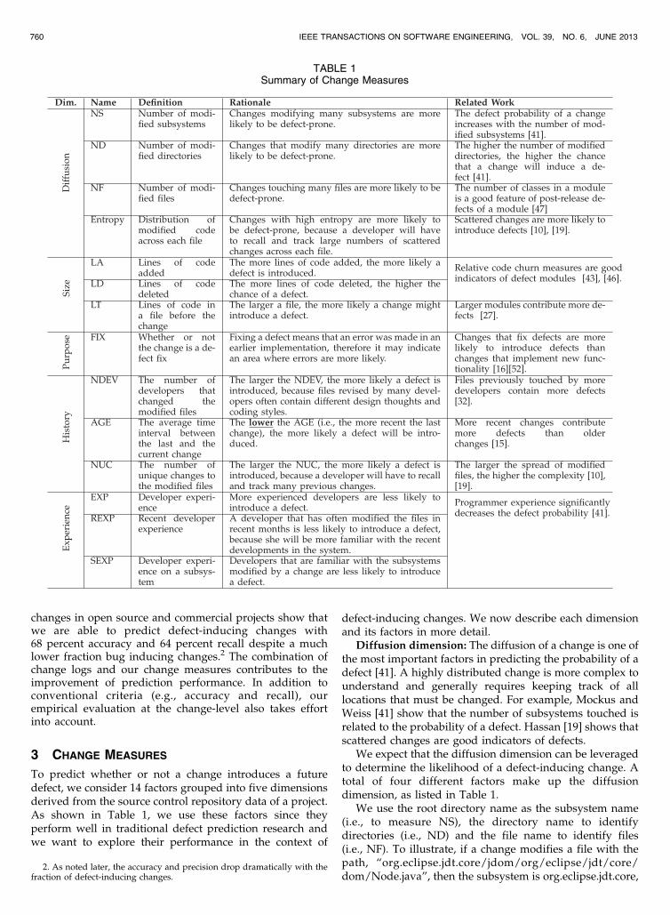
To predict whether or not a change introduces a futuredefect, we consider 14 factors grouped into five dimensionsderived from the source control repository data of a project.As shown in Table 1, we use these factors since theyperform well in traditional defect prediction research andwe want to explore their performance in the context of

defect-inducing changes. We now describe each dimensionand its factors in more detail.

Diffusion dimension: The diffusion of a change is one ofthe most important factors in predicting the probability of adefect [41]. A highly distributed change is more complex tounderstand and generally requires keeping track of alllocations that must be changed. For example, Mockus andWeiss [41] show that the number of subsystems touched isrelated to the probability of a defect. Hassan [19] shows thatscattered changes are good indicators of defects.

We expect that the diffusion dimension can be leveragedto determine the likelihood of a defect-inducing change. Atotal of four different factors make up the diffusiondimension, as listed in Table 1.

We use the root directory name as the subsystem name(i.e., to measure NS), the directory name to identifydirectories (i.e., ND) and the file name to identify files(i.e., NF). To illustrate, if a change modifies a file with thepath, “org.eclipse.jdt.core/jdom/org/eclipse/jdt/core/dom/Node.java”, then the subsystem is org.eclipse.jdt.core,


TABLE 1Summary of Change Measures

2. As noted later, the accuracy and precision drop dramatically with thefraction of defect-inducing changes.

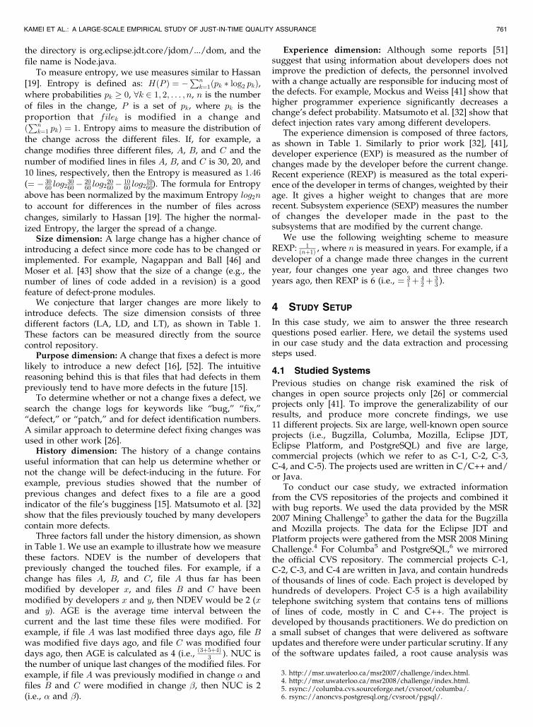
the directory is org.eclipse.jdt.core/jdom/.../dom, and thefile name is Node.java.

To measure entropy, we use measures similar to Hassan[19]. Entropy is defined as: HðP Þ ¼ �

Pnk¼1ðpk � log2 pkÞ,

where probabilities pk � 0, 8k 2 1; 2; . . . ; n, n is the numberof files in the change, P is a set of pk, where pk is theproportion that filek is modified in a change andðPn

k¼1 pkÞ ¼ 1. Entropy aims to measure the distribution ofthe change across the different files. If, for example, achange modifies three different files, A, B, and C and thenumber of modified lines in files A, B, and C is 30, 20, and10 lines, respectively, then the Entropy is measured as 1:46

(¼ � 3060 log2

3060� 20

60 log22060� 10

60 log21060). The formula for Entropy

above has been normalized by the maximum Entropy log2n

to account for differences in the number of files acrosschanges, similarly to Hassan [19]. The higher the normal-ized Entropy, the larger the spread of a change.

Size dimension: A large change has a higher chance ofintroducing a defect since more code has to be changed orimplemented. For example, Nagappan and Ball [46] andMoser et al. [43] show that the size of a change (e.g., thenumber of lines of code added in a revision) is a goodfeature of defect-prone modules.

We conjecture that larger changes are more likely tointroduce defects. The size dimension consists of threedifferent factors (LA, LD, and LT), as shown in Table 1.These factors can be measured directly from the sourcecontrol repository.

Purpose dimension: A change that fixes a defect is morelikely to introduce a new defect [16], [52]. The intuitivereasoning behind this is that files that had defects in thempreviously tend to have more defects in the future [15].

To determine whether or not a change fixes a defect, wesearch the change logs for keywords like “bug,” “fix,”“defect,” or “patch,” and for defect identification numbers.A similar approach to determine defect fixing changes wasused in other work [26].

History dimension: The history of a change containsuseful information that can help us determine whether ornot the change will be defect-inducing in the future. Forexample, previous studies showed that the number ofprevious changes and defect fixes to a file are a goodindicator of the file’s bugginess [15]. Matsumoto et al. [32]show that the files previously touched by many developerscontain more defects.

Three factors fall under the history dimension, as shownin Table 1. We use an example to illustrate how we measurethese factors. NDEV is the number of developers thatpreviously changed the touched files. For example, if achange has files A, B, and C, file A thus far has beenmodified by developer x, and files B and C have beenmodified by developers x and y, then NDEV would be 2 (xand y). AGE is the average time interval between thecurrent and the last time these files were modified. Forexample, if file A was last modified three days ago, file Bwas modified five days ago, and file C was modified fourdays ago, then AGE is calculated as 4 (i.e., ð3þ5þ4Þ

3 ). NUC isthe number of unique last changes of the modified files. Forexample, if file A was previously modified in change � andfiles B and C were modified in change �, then NUC is 2(i.e., � and �).

Experience dimension: Although some reports [51]suggest that using information about developers does notimprove the prediction of defects, the personnel involvedwith a change actually are responsible for inducing most ofthe defects. For example, Mockus and Weiss [41] show thathigher programmer experience significantly decreases achange’s defect probability. Matsumoto et al. [32] show thatdefect injection rates vary among different developers.

The experience dimension is composed of three factors,as shown in Table 1. Similarly to prior work [32], [41],developer experience (EXP) is measured as the number ofchanges made by the developer before the current change.Recent experience (REXP) is measured as the total experi-ence of the developer in terms of changes, weighted by theirage. It gives a higher weight to changes that are morerecent. Subsystem experience (SEXP) measures the numberof changes the developer made in the past to thesubsystems that are modified by the current change.

We use the following weighting scheme to measureREXP: 1

ðnþ1Þ , where n is measured in years. For example, if adeveloper of a change made three changes in the currentyear, four changes one year ago, and three changes twoyears ago, then REXP is 6 (i.e., ¼ 3

1þ 42þ 3

3 ).

4 STUDY SETUP

In this case study, we aim to answer the three researchquestions posed earlier. Here, we detail the systems usedin our case study and the data extraction and processingsteps used.

4.1 Studied Systems

Previous studies on change risk examined the risk ofchanges in open source projects only [26] or commercialprojects only [41]. To improve the generalizability of ourresults, and produce more concrete findings, we use11 different projects. Six are large, well-known open sourceprojects (i.e., Bugzilla, Columba, Mozilla, Eclipse JDT,Eclipse Platform, and PostgreSQL) and five are large,commercial projects (which we refer to as C-1, C-2, C-3,C-4, and C-5). The projects used are written in C/C++ and/or Java.

To conduct our case study, we extracted informationfrom the CVS repositories of the projects and combined itwith bug reports. We used the data provided by the MSR2007 Mining Challenge3 to gather the data for the Bugzillaand Mozilla projects. The data for the Eclipse JDT andPlatform projects were gathered from the MSR 2008 MiningChallenge.4 For Columba5 and PostgreSQL,6 we mirroredthe official CVS repository. The commercial projects C-1,C-2, C-3, and C-4 are written in Java, and contain hundredsof thousands of lines of code. Each project is developed byhundreds of developers. Project C-5 is a high availabilitytelephone switching system that contains tens of millionsof lines of code, mostly in C and C++. The project isdeveloped by thousands practitioners. We do prediction ona small subset of changes that were delivered as softwareupdates and therefore were under particular scrutiny. If anyof the software updates failed, a root cause analysis was


3. http://msr.uwaterloo.ca/msr2007/challenge/index.html.4. http://msr.uwaterloo.ca/msr2008/challenge/index.html.5. rsync://columba.cvs.sourceforge.net/cvsroot/columba/.6. rsync://anoncvs.postgresql.org/cvsroot/pgsql/.

conducted, including the identification of the changecausing the update to fail. We used the subset of changesfrom these analyses to identify defect-inducing changesamong all changes involved in software updates.

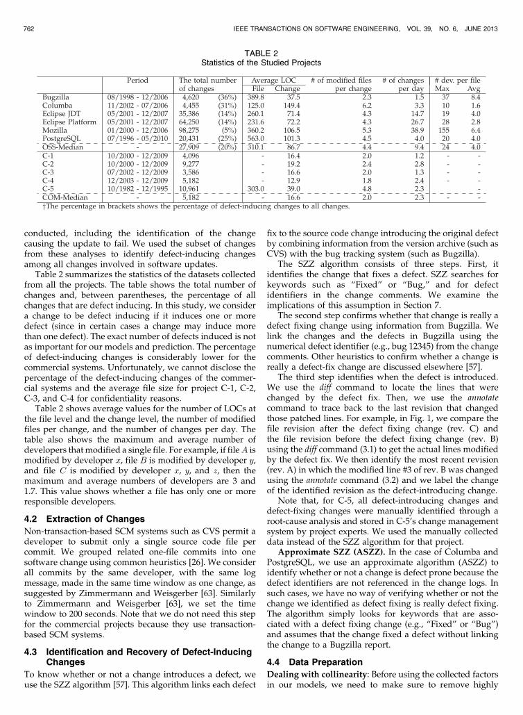
Table 2 summarizes the statistics of the datasets collectedfrom all the projects. The table shows the total number ofchanges and, between parentheses, the percentage of allchanges that are defect inducing. In this study, we considera change to be defect inducing if it induces one or moredefect (since in certain cases a change may induce morethan one defect). The exact number of defects induced is notas important for our models and prediction. The percentageof defect-inducing changes is considerably lower for thecommercial systems. Unfortunately, we cannot disclose thepercentage of the defect-inducing changes of the commer-cial systems and the average file size for project C-1, C-2,C-3, and C-4 for confidentiality reasons.

Table 2 shows average values for the number of LOCs atthe file level and the change level, the number of modifiedfiles per change, and the number of changes per day. Thetable also shows the maximum and average number ofdevelopers that modified a single file. For example, if fileA ismodified by developer x, file B is modified by developer y,and file C is modified by developer x, y, and z, then themaximum and average numbers of developers are 3 and1.7. This value shows whether a file has only one or moreresponsible developers.

4.2 Extraction of Changes

Non-transaction-based SCM systems such as CVS permit adeveloper to submit only a single source code file percommit. We grouped related one-file commits into onesoftware change using common heuristics [26]. We considerall commits by the same developer, with the same logmessage, made in the same time window as one change, assuggested by Zimmermann and Weisgerber [63]. Similarlyto Zimmermann and Weisgerber [63], we set the timewindow to 200 seconds. Note that we do not need this stepfor the commercial projects because they use transaction-based SCM systems.

4.3 Identification and Recovery of Defect-InducingChanges

To know whether or not a change introduces a defect, weuse the SZZ algorithm [57]. This algorithm links each defect

fix to the source code change introducing the original defectby combining information from the version archive (such asCVS) with the bug tracking system (such as Bugzilla).

The SZZ algorithm consists of three steps. First, itidentifies the change that fixes a defect. SZZ searches forkeywords such as “Fixed” or “Bug,” and for defectidentifiers in the change comments. We examine theimplications of this assumption in Section 7.

The second step confirms whether that change is really adefect fixing change using information from Bugzilla. Welink the changes and the defects in Bugzilla using thenumerical defect identifier (e.g., bug 12345) from the changecomments. Other heuristics to confirm whether a change isreally a defect-fix change are discussed elsewhere [57].

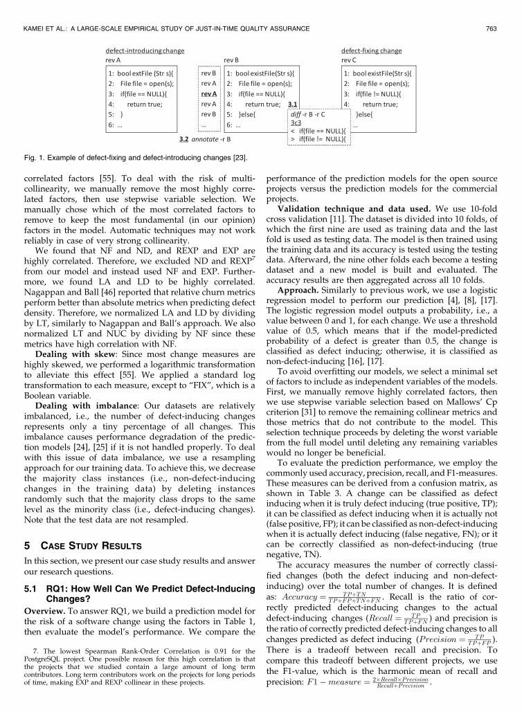
The third step identifies when the defect is introduced.We use the diff command to locate the lines that werechanged by the defect fix. Then, we use the annotatecommand to trace back to the last revision that changedthose patched lines. For example, in Fig. 1, we compare thefile revision after the defect fixing change (rev. C) andthe file revision before the defect fixing change (rev. B)using the diff command (3.1) to get the actual lines modifiedby the defect fix. We then identify the most recent revision(rev. A) in which the modified line #3 of rev. B was changedusing the annotate command (3.2) and we label the changeof the identified revision as the defect-introducing change.

Note that, for C-5, all defect-introducing changes anddefect-fixing changes were manually identified through aroot-cause analysis and stored in C-5’s change managementsystem by project experts. We used the manually collecteddata instead of the SZZ algorithm for that project.

Approximate SZZ (ASZZ). In the case of Columba andPostgreSQL, we use an approximate algorithm (ASZZ) toidentify whether or not a change is defect prone because thedefect identifiers are not referenced in the change logs. Insuch cases, we have no way of verifying whether or not thechange we identified as defect fixing is really defect fixing.The algorithm simply looks for keywords that are asso-ciated with a defect fixing change (e.g., “Fixed” or “Bug”)and assumes that the change fixed a defect without linkingthe change to a Bugzilla report.

4.4 Data Preparation

Dealing with collinearity: Before using the collected factorsin our models, we need to make sure to remove highly


TABLE 2Statistics of the Studied Projects

correlated factors [55]. To deal with the risk of multi-collinearity, we manually remove the most highly corre-lated factors, then use stepwise variable selection. Wemanually chose which of the most correlated factors toremove to keep the most fundamental (in our opinion)factors in the model. Automatic techniques may not workreliably in case of very strong collinearity.

We found that NF and ND, and REXP and EXP arehighly correlated. Therefore, we excluded ND and REXP7

from our model and instead used NF and EXP. Further-more, we found LA and LD to be highly correlated.Nagappan and Ball [46] reported that relative churn metricsperform better than absolute metrics when predicting defectdensity. Therefore, we normalized LA and LD by dividingby LT, similarly to Nagappan and Ball’s approach. We alsonormalized LT and NUC by dividing by NF since thesemetrics have high correlation with NF.

Dealing with skew: Since most change measures arehighly skewed, we performed a logarithmic transformationto alleviate this effect [55]. We applied a standard logtransformation to each measure, except to “FIX”, which is aBoolean variable.

Dealing with imbalance: Our datasets are relativelyimbalanced, i.e., the number of defect-inducing changesrepresents only a tiny percentage of all changes. Thisimbalance causes performance degradation of the predic-tion models [24], [25] if it is not handled properly. To dealwith this issue of data imbalance, we use a resamplingapproach for our training data. To achieve this, we decreasethe majority class instances (i.e., non-defect-inducingchanges in the training data) by deleting instancesrandomly such that the majority class drops to the samelevel as the minority class (i.e., defect-inducing changes).Note that the test data are not resampled.

5 CASE STUDY RESULTS

In this section, we present our case study results and answerour research questions.

5.1 RQ1: How Well Can We Predict Defect-InducingChanges?

Overview. To answer RQ1, we build a prediction model forthe risk of a software change using the factors in Table 1,then evaluate the model’s performance. We compare the

performance of the prediction models for the open sourceprojects versus the prediction models for the commercialprojects.

Validation technique and data used. We use 10-foldcross validation [11]. The dataset is divided into 10 folds, ofwhich the first nine are used as training data and the lastfold is used as testing data. The model is then trained usingthe training data and its accuracy is tested using the testingdata. Afterward, the nine other folds each become a testingdataset and a new model is built and evaluated. Theaccuracy results are then aggregated across all 10 folds.

Approach. Similarly to previous work, we use a logisticregression model to perform our prediction [4], [8], [17].The logistic regression model outputs a probability, i.e., avalue between 0 and 1, for each change. We use a thresholdvalue of 0.5, which means that if the model-predictedprobability of a defect is greater than 0.5, the change isclassified as defect inducing; otherwise, it is classified asnon-defect-inducing [16], [17].

To avoid overfitting our models, we select a minimal setof factors to include as independent variables of the models.First, we manually remove highly correlated factors, thenwe use stepwise variable selection based on Mallows’ Cpcriterion [31] to remove the remaining collinear metrics andthose metrics that do not contribute to the model. Thisselection technique proceeds by deleting the worst variablefrom the full model until deleting any remaining variableswould no longer be beneficial.

To evaluate the prediction performance, we employ thecommonly used accuracy, precision, recall, and F1-measures.These measures can be derived from a confusion matrix, asshown in Table 3. A change can be classified as defectinducing when it is truly defect inducing (true positive, TP);it can be classified as defect inducing when it is actually not(false positive, FP); it can be classified as non-defect-inducingwhen it is actually defect inducing (false negative, FN); or itcan be correctly classified as non-defect-inducing (truenegative, TN).

The accuracy measures the number of correctly classi-fied changes (both the defect inducing and non-defect-inducing) over the total number of changes. It is definedas: Accuracy ¼ TPþTN

TPþFPþTNþFN . Recall is the ratio of cor-rectly predicted defect-inducing changes to the actualdefect-inducing changes (Recall ¼ TP

TPþFN ) and precision isthe ratio of correctly predicted defect-inducing changes to allchanges predicted as defect inducing (Precision ¼ TP

TPþFP ).There is a tradeoff between recall and precision. Tocompare this tradeoff between different projects, we usethe F1-value, which is the harmonic mean of recall andprecision: F1�measure ¼ 2�Recall�Precision

RecallþPrecision .


Fig. 1. Example of defect-fixing and defect-introducing changes [23].

7. The lowest Spearman Rank-Order Correlation is 0.91 for thePostgreSQL project. One possible reason for this high correlation is thatthe projects that we studied contain a large amount of long termcontributors. Long term contributors work on the projects for long periodsof time, making EXP and REXP collinear in these projects.

These criteria (e.g., precision and recall) depend on theparticular threshold used for the classification. Choosinganother threshold might lead to different results; hence wecalculated the measures for different thresholds. To get anoverall idea of the performance across thresholds, weadditionally use the area under the curve (AUC) of ROC(the receiver operating characteristics) [28]. The range ofAUC is ½0; 1� and larger AUC value indicates betterprediction performance. Any predictor achieving AUCabove 0.5 is more effective than the random predictor.The advantage of the AUC of ROC is its robustness towardimbalanced data since the ROC is obtained by varying theclassification threshold over all possible values.

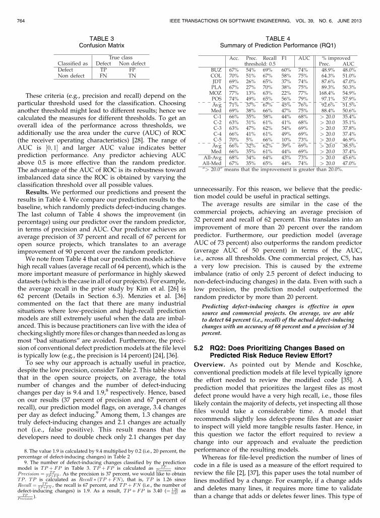
Results. We performed our predictions and present theresults in Table 4. We compare our prediction results to thebaseline, which randomly predicts defect-inducing changes.The last column of Table 4 shows the improvement (inpercentage) using our predictor over the random predictor,in terms of precision and AUC. Our predictor achieves anaverage precision of 37 percent and recall of 67 percent foropen source projects, which translates to an averageimprovement of 90 percent over the random predictor.

We note from Table 4 that our prediction models achievehigh recall values (average recall of 64 percent), which is themore important measure of performance in highly skeweddatasets (which is the case in all of our projects). For example,the average recall in the prior study by Kim et al. [26] is62 percent (Details in Section 6.3). Menzies et al. [36]commented on the fact that there are many industrialsituations where low-precision and high-recall predictionmodels are still extremely useful when the data are imbal-anced. This is because practitioners can live with the idea ofchecking slightly more files or changes than needed as long asmost “bad situations” are avoided. Furthermore, the preci-sion of conventional defect prediction models at the file levelis typically low (e.g., the precision is 14 percent) [24], [36].

To see why our approach is actually useful in practice,despite the low precision, consider Table 2. This table showsthat in the open source projects, on average, the totalnumber of changes and the number of defect-inducingchanges per day is 9.4 and 1.9,8 respectively. Hence, basedon our results (37 percent of precision and 67 percent ofrecall), our prediction model flags, on average, 3.4 changesper day as defect inducing.9 Among them, 1.3 changes aretruly defect-inducing changes and 2.1 changes are actuallynot (i.e., false positive). This result means that thedevelopers need to double check only 2.1 changes per day

unnecessarily. For this reason, we believe that the predic-tion model could be useful in practical settings.

The average results are similar in the case of thecommercial projects, achieving an average precision of32 percent and recall of 62 percent. This translates into animprovement of more than 20 percent over the randompredictor. Furthermore, our prediction model (averageAUC of 73 percent) also outperforms the random predictor(average AUC of 50 percent) in terms of the AUC,i.e., across all thresholds. One commercial project, C5, hasa very low precision. This is caused by the extremeimbalance (ratio of only 2.5 percent of defect inducing tonon-defect-inducing changes) in the data. Even with such alow precision, the prediction model outperformed therandom predictor by more than 20 percent.

Predicting defect-inducing changes is effective in opensource and commercial projects. On average, we are ableto detect 64 percent (i.e., recall) of the actual defect-inducingchanges with an accuracy of 68 percent and a precision of 34percent.

5.2 RQ2: Does Prioritizing Changes Based onPredicted Risk Reduce Review Effort?

Overview. As pointed out by Mende and Koschke,conventional prediction models at file level typically ignorethe effort needed to review the modified code [35]. Aprediction model that prioritizes the largest files as mostdefect prone would have a very high recall, i.e., those fileslikely contain the majority of defects, yet inspecting all thosefiles would take a considerable time. A model thatrecommends slightly less defect-prone files that are easierto inspect will yield more tangible results faster. Hence, inthis question we factor the effort required to review achange into our approach and evaluate the predictionperformance of the resulting models.

Whereas for file-level prediction the number of lines ofcode in a file is used as a measure of the effort required toreview the file [2], [37], this paper uses the total number oflines modified by a change. For example, if a change addsand deletes many lines, it requires more time to validatethan a change that adds or deletes fewer lines. This type of


TABLE 4Summary of Prediction Performance (RQ1)

8. The value 1.9 is calculated by 9.4 multiplied by 0.2 (i.e., 20 percent, thepercentage of defect-inducing changes) in Table 2

9. The number of defect-inducing changes classified by the predictionmodel is TP þ FP in Table 3. TP þ FP is calculated as TP

Precision sincePrecision ¼ TP

TPþFP . As the precision is 37 percent, we would like to obtainTP . TP is calculated as Recall � ðTP þ FNÞ, that is, TP is 1.26 sinceRecall ¼ TP

TPþFN , the recall is 67 percent, and TP þ FN (i.e., the number ofdefect-inducing changes) is 1.9. As a result, TP þ FP is 3.40 (¼ 1:26

0:37 asTP

Precision ).

TABLE 3Confusion Matrix

effort-aware prediction offers a more practical adoption-oriented view of defect prediction results.

Approach. For our effort-aware evaluation, we first buildnaive models based on our RQ1 models as a first attempttoward effort-aware models. We then build customizedeffort-aware models, and compare those to random modelsthat we use as a baseline.10 Similarly to RQ2, we use 10-foldcross validation as validation technique.

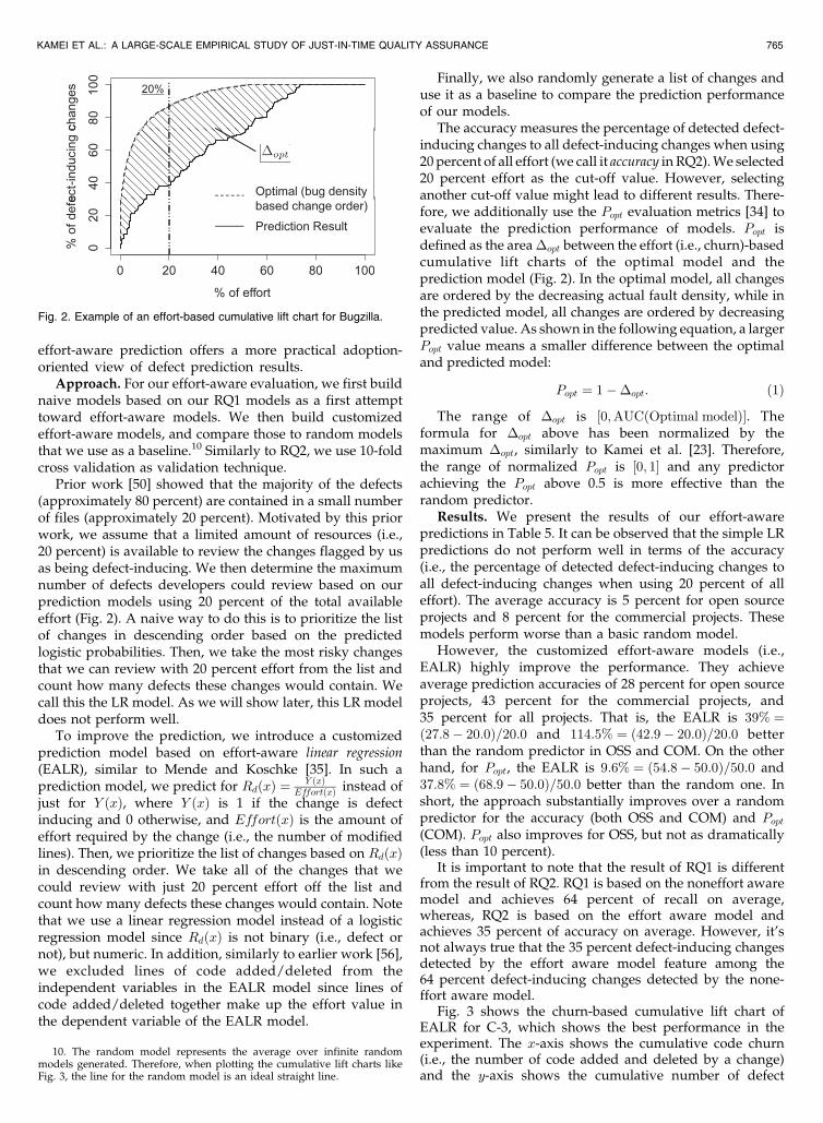
Prior work [50] showed that the majority of the defects(approximately 80 percent) are contained in a small numberof files (approximately 20 percent). Motivated by this priorwork, we assume that a limited amount of resources (i.e.,20 percent) is available to review the changes flagged by usas being defect-inducing. We then determine the maximumnumber of defects developers could review based on ourprediction models using 20 percent of the total availableeffort (Fig. 2). A naive way to do this is to prioritize the listof changes in descending order based on the predictedlogistic probabilities. Then, we take the most risky changesthat we can review with 20 percent effort from the list andcount how many defects these changes would contain. Wecall this the LR model. As we will show later, this LR modeldoes not perform well.

To improve the prediction, we introduce a customizedprediction model based on effort-aware linear regression(EALR), similar to Mende and Koschke [35]. In such aprediction model, we predict for RdðxÞ ¼ Y ðxÞ

EffortðxÞ instead ofjust for Y ðxÞ, where Y ðxÞ is 1 if the change is defectinducing and 0 otherwise, and EffortðxÞ is the amount ofeffort required by the change (i.e., the number of modifiedlines). Then, we prioritize the list of changes based on RdðxÞin descending order. We take all of the changes that wecould review with just 20 percent effort off the list andcount how many defects these changes would contain. Notethat we use a linear regression model instead of a logisticregression model since RdðxÞ is not binary (i.e., defect ornot), but numeric. In addition, similarly to earlier work [56],we excluded lines of code added/deleted from theindependent variables in the EALR model since lines ofcode added/deleted together make up the effort value inthe dependent variable of the EALR model.

Finally, we also randomly generate a list of changes anduse it as a baseline to compare the prediction performanceof our models.

The accuracy measures the percentage of detected defect-inducing changes to all defect-inducing changes when using20 percent of all effort (we call it accuracy in RQ2). We selected20 percent effort as the cut-off value. However, selectinganother cut-off value might lead to different results. There-fore, we additionally use the Popt evaluation metrics [34] toevaluate the prediction performance of models. Popt isdefined as the area �opt between the effort (i.e., churn)-basedcumulative lift charts of the optimal model and theprediction model (Fig. 2). In the optimal model, all changesare ordered by the decreasing actual fault density, while inthe predicted model, all changes are ordered by decreasingpredicted value. As shown in the following equation, a largerPopt value means a smaller difference between the optimaland predicted model:

Popt ¼ 1��opt: ð1Þ

The range of �opt is ½0;AUCðOptimal modelÞ�. Theformula for �opt above has been normalized by themaximum �opt, similarly to Kamei et al. [23]. Therefore,the range of normalized Popt is ½0; 1� and any predictorachieving the Popt above 0.5 is more effective than therandom predictor.

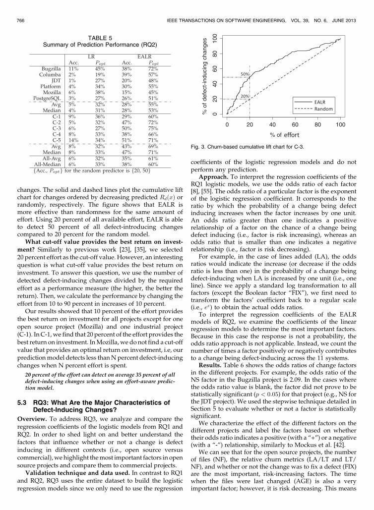
Results. We present the results of our effort-awarepredictions in Table 5. It can be observed that the simple LRpredictions do not perform well in terms of the accuracy(i.e., the percentage of detected defect-inducing changes toall defect-inducing changes when using 20 percent of alleffort). The average accuracy is 5 percent for open sourceprojects and 8 percent for the commercial projects. Thesemodels perform worse than a basic random model.

However, the customized effort-aware models (i.e.,EALR) highly improve the performance. They achieveaverage prediction accuracies of 28 percent for open sourceprojects, 43 percent for the commercial projects, and35 percent for all projects. That is, the EALR is 39% ¼ð27:8� 20:0Þ=20:0 and 114:5% ¼ ð42:9� 20:0Þ=20:0 betterthan the random predictor in OSS and COM. On the otherhand, for Popt, the EALR is 9:6% ¼ ð54:8� 50:0Þ=50:0 and37:8% ¼ ð68:9� 50:0Þ=50:0 better than the random one. Inshort, the approach substantially improves over a randompredictor for the accuracy (both OSS and COM) and Popt(COM). Popt also improves for OSS, but not as dramatically(less than 10 percent).

It is important to note that the result of RQ1 is differentfrom the result of RQ2. RQ1 is based on the noneffort awaremodel and achieves 64 percent of recall on average,whereas, RQ2 is based on the effort aware model andachieves 35 percent of accuracy on average. However, it’snot always true that the 35 percent defect-inducing changesdetected by the effort aware model feature among the64 percent defect-inducing changes detected by the none-ffort aware model.

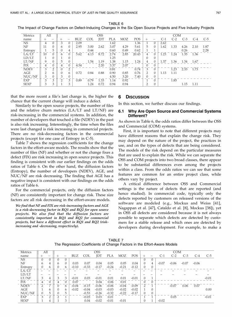
Fig. 3 shows the churn-based cumulative lift chart ofEALR for C-3, which shows the best performance in theexperiment. The x-axis shows the cumulative code churn(i.e., the number of code added and deleted by a change)and the y-axis shows the cumulative number of defect


Fig. 2. Example of an effort-based cumulative lift chart for Bugzilla.

10. The random model represents the average over infinite randommodels generated. Therefore, when plotting the cumulative lift charts likeFig. 3, the line for the random model is an ideal straight line.

changes. The solid and dashed lines plot the cumulative liftchart for changes ordered by decreasing predicted RdðxÞ orrandomly, respectively. The figure shows that EALR ismore effective than randomness for the same amount ofeffort. Using 20 percent of all available effort, EALR is ableto detect 50 percent of all defect-introducing changescompared to 20 percent for the random model.

What cut-off value provides the best return on invest-

ment? Similarly to previous work [23], [35], we selected20 percent effort as the cut-off value. However, an interestingquestion is what cut-off value provides the best return oninvestment. To answer this question, we use the number ofdetected defect-inducing changes divided by the requiredeffort as a performance measure (the higher, the better thereturn). Then, we calculate the performance by changing theeffort from 10 to 90 percent in increases of 10 percent.

Our results showed that 10 percent of the effort providesthe best return on investment for all projects except for oneopen source project (Mozilla) and one industrial project(C-1). In C-1, we find that 20 percent of the effort provides thebest return on investment. In Mozilla, we do not find a cut-offvalue that provides an optimal return on investment, i.e, ourprediction model detects less than N percent defect-inducingchanges when N percent effort is spent.

20 percent of the effort can detect on average 35 percent of alldefect-inducing changes when using an effort-aware predic-tion model.

5.3 RQ3: What Are the Major Characteristics ofDefect-Inducing Changes?

Overview. To address RQ3, we analyze and compare theregression coefficients of the logistic models from RQ1 andRQ2. In order to shed light on and better understand thefactors that influence whether or not a change is defectinducing in different contexts (i.e., open source versuscommercial), we highlight the most important factors in opensource projects and compare them to commercial projects.

Validation technique and data used. In contrast to RQ1and RQ2, RQ3 uses the entire dataset to build the logisticregression models since we only need to use the regression

coefficients of the logistic regression models and do notperform any prediction.

Approach. To interpret the regression coefficients of theRQ1 logistic models, we use the odds ratio of each factor[8], [55]. The odds ratio of a particular factor is the exponentof the logistic regression coefficient. It corresponds to theratio by which the probability of a change being defectinducing increases when the factor increases by one unit.An odds ratio greater than one indicates a positiverelationship of a factor on the chance of a change beingdefect inducing (i.e., factor is risk increasing), whereas anodds ratio that is smaller than one indicates a negativerelationship (i.e., factor is risk decreasing).

For example, in the case of lines added (LA), the oddsratios would indicate the increase (or decrease if the oddsratio is less than one) in the probability of a change beingdefect-inducing when LA is increased by one unit (i.e., oneline). Since we apply a standard log transformation to allfactors (except the Boolean factor “FIX”), we first need totransform the factors’ coefficient back to a regular scale(i.e., ex) to obtain the actual odds ratios.

To interpret the regression coefficients of the EALRmodels of RQ2, we examine the coefficients of the linearregression models to determine the most important factors.Because in this case the response is not a probability, theodds ratio approach is not applicable. Instead, we count thenumber of times a factor positively or negatively contributesto a change being defect-inducing across the 11 systems.

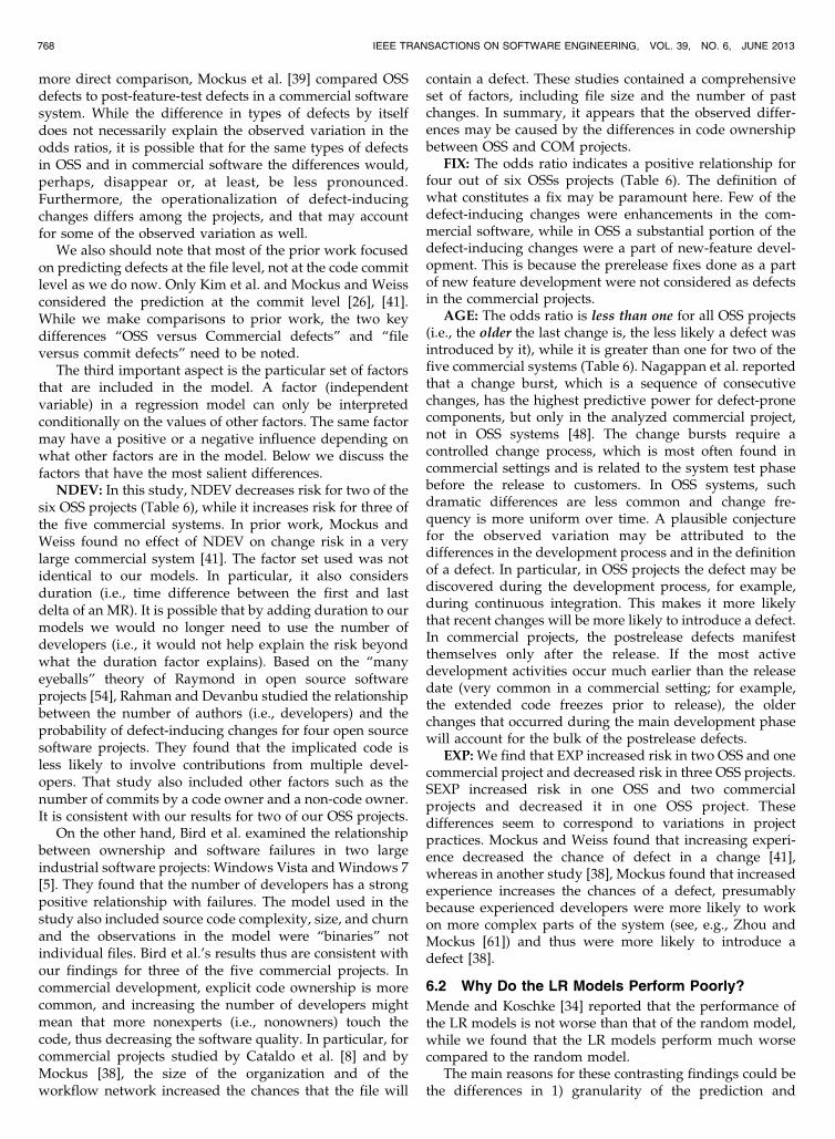
Results. Table 6 shows the odds ratios of change factorsin the different projects. For example, the odds ratio of theNS factor in the Bugzilla project is 2.09. In the cases wherethe odds ratio value is blank, the factor did not prove to bestatistically significant (p < 0:05) for that project (e.g., NS forthe JDT project). We used the stepwise technique detailed inSection 5 to evaluate whether or not a factor is statisticallysignificant.

We characterize the effect of the different factors on thedifferent projects and label the factors based on whethertheir odds ratio indicates a positive (with a “+”) or a negative(with a “-”) relationship, similarly to Mockus et al. [42].

We can see that for the open source projects, the numberof files (NF), the relative churn metrics (LA/LT and LT/NF), and whether or not the change was to fix a defect (FIX)are the most important, risk-increasing factors. The timewhen the files were last changed (AGE) is also a veryimportant factor; however, it is risk decreasing. This means


Fig. 3. Churn-based cumulative lift chart for C-3.

TABLE 5Summary of Prediction Performance (RQ2)

that the more recent a file’s last change is, the higher thechance that the current change will induce a defect.

Similarly to the open source projects, the number of filesand the relative churn metrics (LA/LT and LT/NF) arerisk-increasing in the commercial systems. In addition, thenumber of developers that touched a file (NDEV) in the pastis also risk increasing. Interestingly, the time when the fileswere last changed is risk increasing in commercial projects.There are no risk-decreasing factors in the commercialprojects (except for one case of Entropy in C-5).

Table 7 shows the regression coefficients for the changefactors in the effort-aware models. The results show that thenumber of files (NF) and whether or not the change fixes adefect (FIX) are risk increasing in open source projects. Thisfinding is consistent with our earlier findings on the oddsratios of Table 6. On the other hand, the diffusion factors(Entropy), the number of developers (NDEV), AGE, andNUC/NF are risk decreasing. The finding that AGE has anegative impact is consistent with our findings on the oddsratios of Table 6.

For the commercial projects, only the diffusion factors

(NF) are consistently important for change risk. These size

factors are all risk decreasing in the effort-aware models.

We find that NF and FIX are risk-increasing factors and AGEis a risk-decreasing factor in RQ1 and RQ2 for open sourceprojects. We also find that the diffusion factors areconsistently important in RQ1 and RQ2 for commercialprojects, but have a different effect in RQ1 and RQ2 (risk-increasing and -decreasing, respectively).

6 DISCUSSION

In this section, we further discuss our findings.

6.1 Why Are Open Source and Commercial SystemsDifferent?

As shown in Table 6, the odds ratios differ between the OSSand Commercial (COM) systems.

First, it is important to note that different projects mayhave different reasons that explain the change risk. Theymay depend on the nature of the project, the practices inuse, and on the types of defects that are being considered.The models of the risk depend on the particular measuresthat are used to explain the risk. While we can separate theOSS and COM projects into two broad classes, there appearto be substantial differences even among the projectswithin a class. From the odds ratios we can see that somefeatures are common for an entire project class, whileothers vary by project.

A critical difference between OSS and Commercialsettings is the nature of defects that are reported (andhence studied). In commercial code, typically only thedefects reported by customers on released versions of thesoftware are modeled (e.g., Mockus and Weiss [41],Nagappan et al. [47], Cataldo et al. [8], Mockus [38]), yetin OSS all defects are considered because it is not alwayspossible to separate which defects are detected by custo-mers for a stable release and which ones are detected bydevelopers during development. For example, to make a


TABLE 6The Impact of Change Factors on Defect-Inducing Changes in the Six Open Source Projects and Five Industry Projects

TABLE 7The Regression Coefficients of Change Factors in the Effort-Aware Models

more direct comparison, Mockus et al. [39] compared OSSdefects to post-feature-test defects in a commercial softwaresystem. While the difference in types of defects by itselfdoes not necessarily explain the observed variation in theodds ratios, it is possible that for the same types of defectsin OSS and in commercial software the differences would,perhaps, disappear or, at least, be less pronounced.Furthermore, the operationalization of defect-inducingchanges differs among the projects, and that may accountfor some of the observed variation as well.

We also should note that most of the prior work focusedon predicting defects at the file level, not at the code commitlevel as we do now. Only Kim et al. and Mockus and Weissconsidered the prediction at the commit level [26], [41].While we make comparisons to prior work, the two keydifferences “OSS versus Commercial defects” and “fileversus commit defects” need to be noted.

The third important aspect is the particular set of factorsthat are included in the model. A factor (independentvariable) in a regression model can only be interpretedconditionally on the values of other factors. The same factormay have a positive or a negative influence depending onwhat other factors are in the model. Below we discuss thefactors that have the most salient differences.

NDEV: In this study, NDEV decreases risk for two of thesix OSS projects (Table 6), while it increases risk for three ofthe five commercial systems. In prior work, Mockus andWeiss found no effect of NDEV on change risk in a verylarge commercial system [41]. The factor set used was notidentical to our models. In particular, it also considersduration (i.e., time difference between the first and lastdelta of an MR). It is possible that by adding duration to ourmodels we would no longer need to use the number ofdevelopers (i.e., it would not help explain the risk beyondwhat the duration factor explains). Based on the “manyeyeballs” theory of Raymond in open source softwareprojects [54], Rahman and Devanbu studied the relationshipbetween the number of authors (i.e., developers) and theprobability of defect-inducing changes for four open sourcesoftware projects. They found that the implicated code isless likely to involve contributions from multiple devel-opers. That study also included other factors such as thenumber of commits by a code owner and a non-code owner.It is consistent with our results for two of our OSS projects.

On the other hand, Bird et al. examined the relationshipbetween ownership and software failures in two largeindustrial software projects: Windows Vista and Windows 7[5]. They found that the number of developers has a strongpositive relationship with failures. The model used in thestudy also included source code complexity, size, and churnand the observations in the model were “binaries” notindividual files. Bird et al.’s results thus are consistent withour findings for three of the five commercial projects. Incommercial development, explicit code ownership is morecommon, and increasing the number of developers mightmean that more nonexperts (i.e., nonowners) touch thecode, thus decreasing the software quality. In particular, forcommercial projects studied by Cataldo et al. [8] and byMockus [38], the size of the organization and of theworkflow network increased the chances that the file will

contain a defect. These studies contained a comprehensiveset of factors, including file size and the number of pastchanges. In summary, it appears that the observed differ-ences may be caused by the differences in code ownershipbetween OSS and COM projects.

FIX: The odds ratio indicates a positive relationship forfour out of six OSSs projects (Table 6). The definition ofwhat constitutes a fix may be paramount here. Few of thedefect-inducing changes were enhancements in the com-mercial software, while in OSS a substantial portion of thedefect-inducing changes were a part of new-feature devel-opment. This is because the prerelease fixes done as a partof new feature development were not considered as defectsin the commercial projects.

AGE: The odds ratio is less than one for all OSS projects(i.e., the older the last change is, the less likely a defect wasintroduced by it), while it is greater than one for two of thefive commercial systems (Table 6). Nagappan et al. reportedthat a change burst, which is a sequence of consecutivechanges, has the highest predictive power for defect-pronecomponents, but only in the analyzed commercial project,not in OSS systems [48]. The change bursts require acontrolled change process, which is most often found incommercial settings and is related to the system test phasebefore the release to customers. In OSS systems, suchdramatic differences are less common and change fre-quency is more uniform over time. A plausible conjecturefor the observed variation may be attributed to thedifferences in the development process and in the definitionof a defect. In particular, in OSS projects the defect may bediscovered during the development process, for example,during continuous integration. This makes it more likelythat recent changes will be more likely to introduce a defect.In commercial projects, the postrelease defects manifestthemselves only after the release. If the most activedevelopment activities occur much earlier than the releasedate (very common in a commercial setting; for example,the extended code freezes prior to release), the olderchanges that occurred during the main development phasewill account for the bulk of the postrelease defects.

EXP: We find that EXP increased risk in two OSS and onecommercial project and decreased risk in three OSS projects.SEXP increased risk in one OSS and two commercialprojects and decreased it in one OSS project. Thesedifferences seem to correspond to variations in projectpractices. Mockus and Weiss found that increasing experi-ence decreased the chance of defect in a change [41],whereas in another study [38], Mockus found that increasedexperience increases the chances of a defect, presumablybecause experienced developers were more likely to workon more complex parts of the system (see, e.g., Zhou andMockus [61]) and thus were more likely to introduce adefect [38].

6.2 Why Do the LR Models Perform Poorly?

Mende and Koschke [34] reported that the performance ofthe LR models is not worse than that of the random model,while we found that the LR models perform much worsecompared to the random model.

The main reasons for these contrasting findings could bethe differences in 1) granularity of the prediction and


2) prediction target. Mende et al.’s prediction granularity is a

file, while our prediction granularity is an individual change.

Changes cover small parts of multiple files, while files are

larger and more cohesive. Target-wise, Mende et al. predict

the number of defects in a file, while we predict whether or not

a change introduces a defect, i.e., whether or not the number

of defects in a change is at least one. Whether we spend a lot

of effort on a large change or a little effort on a smaller

change, if either change has at least one defect, they are

equally buggy from the point of view of our models.

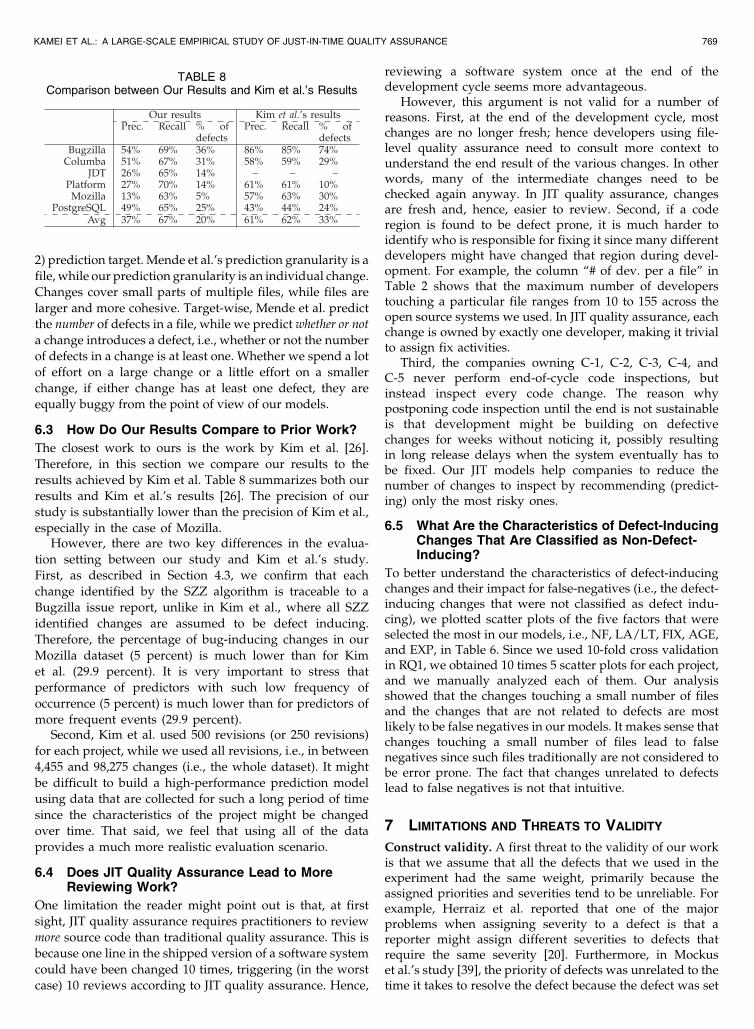
6.3 How Do Our Results Compare to Prior Work?

The closest work to ours is the work by Kim et al. [26].

Therefore, in this section we compare our results to the

results achieved by Kim et al. Table 8 summarizes both our

results and Kim et al.’s results [26]. The precision of our

study is substantially lower than the precision of Kim et al.,

especially in the case of Mozilla.However, there are two key differences in the evalua-

tion setting between our study and Kim et al.’s study.

First, as described in Section 4.3, we confirm that each

change identified by the SZZ algorithm is traceable to a

Bugzilla issue report, unlike in Kim et al., where all SZZ

identified changes are assumed to be defect inducing.

Therefore, the percentage of bug-inducing changes in our

Mozilla dataset (5 percent) is much lower than for Kim

et al. (29.9 percent). It is very important to stress that

performance of predictors with such low frequency of

occurrence (5 percent) is much lower than for predictors of

more frequent events (29.9 percent).Second, Kim et al. used 500 revisions (or 250 revisions)

for each project, while we used all revisions, i.e., in between

4,455 and 98,275 changes (i.e., the whole dataset). It might

be difficult to build a high-performance prediction model

using data that are collected for such a long period of time

since the characteristics of the project might be changed

over time. That said, we feel that using all of the data

provides a much more realistic evaluation scenario.

6.4 Does JIT Quality Assurance Lead to MoreReviewing Work?

One limitation the reader might point out is that, at first

sight, JIT quality assurance requires practitioners to review

more source code than traditional quality assurance. This is

because one line in the shipped version of a software system

could have been changed 10 times, triggering (in the worst

case) 10 reviews according to JIT quality assurance. Hence,

reviewing a software system once at the end of thedevelopment cycle seems more advantageous.

However, this argument is not valid for a number ofreasons. First, at the end of the development cycle, mostchanges are no longer fresh; hence developers using file-level quality assurance need to consult more context tounderstand the end result of the various changes. In otherwords, many of the intermediate changes need to bechecked again anyway. In JIT quality assurance, changesare fresh and, hence, easier to review. Second, if a coderegion is found to be defect prone, it is much harder toidentify who is responsible for fixing it since many differentdevelopers might have changed that region during devel-opment. For example, the column “# of dev. per a file” inTable 2 shows that the maximum number of developerstouching a particular file ranges from 10 to 155 across theopen source systems we used. In JIT quality assurance, eachchange is owned by exactly one developer, making it trivialto assign fix activities.

Third, the companies owning C-1, C-2, C-3, C-4, andC-5 never perform end-of-cycle code inspections, butinstead inspect every code change. The reason whypostponing code inspection until the end is not sustainableis that development might be building on defectivechanges for weeks without noticing it, possibly resultingin long release delays when the system eventually has tobe fixed. Our JIT models help companies to reduce thenumber of changes to inspect by recommending (predict-ing) only the most risky ones.

6.5 What Are the Characteristics of Defect-InducingChanges That Are Classified as Non-Defect-Inducing?

To better understand the characteristics of defect-inducingchanges and their impact for false-negatives (i.e., the defect-inducing changes that were not classified as defect indu-cing), we plotted scatter plots of the five factors that wereselected the most in our models, i.e., NF, LA/LT, FIX, AGE,and EXP, in Table 6. Since we used 10-fold cross validationin RQ1, we obtained 10 times 5 scatter plots for each project,and we manually analyzed each of them. Our analysisshowed that the changes touching a small number of filesand the changes that are not related to defects are mostlikely to be false negatives in our models. It makes sense thatchanges touching a small number of files lead to falsenegatives since such files traditionally are not considered tobe error prone. The fact that changes unrelated to defectslead to false negatives is not that intuitive.

7 LIMITATIONS AND THREATS TO VALIDITY

Construct validity. A first threat to the validity of our workis that we assume that all the defects that we used in theexperiment had the same weight, primarily because theassigned priorities and severities tend to be unreliable. Forexample, Herraiz et al. reported that one of the majorproblems when assigning severity to a defect is that areporter might assign different severities to defects thatrequire the same severity [20]. Furthermore, in Mockuset al.’s study [39], the priority of defects was unrelated to thetime it takes to resolve the defect because the defect was set


TABLE 8Comparison between Our Results and Kim et al.’s Results

by reporters who had less experience than core developers.The work of Shihab et al. focused on determining the mostimportant defects (breakages and surprises) [56], but thatapproach could not be applied to all the projects we areconsidering in this work. In any case, note that all the defectsthat we studied were fixed by the developers and thereforewere at least important enough to be fixed.

For CVS, we grouped related one file commits into onesoftware change using common heuristics [63]. Thesecommon heuristics seem to fit well into our researchenvironment since the changes that we consider are finegrained and we have access to the commit messages in theCVS repositories. If the changes would have been coarsegrained (e.g., a transaction for one month), with no access tocommit messages, Vanya et al.’s approach could be moreapplicable [58].

External validity. Although we use datasets collectedfrom 11 large, long-lived systems (six open source and fivecommercial projects), these projects might not be represen-tative of all projects out there. However, since they cover awide range of domains and sizes, we believe that our worksignificantly contributes to the validation of empiricalknowledge about Just-In-Time quality assurance andeffort-aware models.

There may be other features that we did not measure. Forexample, we expect that the type of changes (e.g.,refactoring [43], [53]), the role of the developer whomodified the file (e.g., core or not), and the number ofdefect-inducing changes in which the files have beentouched in the past might influence the probability of adefect. Further studies using other factors might furtherimprove our predictions.

Internal validity. The SZZ algorithm is commonly usedin defect prediction research [26], [43], but SZZ has its ownlimitations. For example, if a defect is not recorded in theCVS log comment or the keywords for defect identifiers thatwe use (e.g., Bug and Fix [24]) do not cover those used inthe comment, there is no way of mapping the defect back tothe defect-inducing change. We believe that the usage of anapproach to recover missing links [59] is required toimprove the accuracy of the SZZ algorithm to identifydefect-inducing changes from repositories.

This study uses the number of lines of code modified in achange as a measure of the effort required to review achange, similarly to Mende and Koschke [35]. At theminimum, the number of LoC changed represents a lowerbound for the effort since at least the changes themselvesshould be checked during review before consulting otherfiles. This assumption is still an open question for futurework. Also, replicated studies using other measures of effortwill be useful to evaluate the generalizability of our findings.

Similarly to previous work [14], [32], [40], [41], we usethe number of changes as the developer’s project experi-ence. Furthermore, we believe that the number of commitsis a better measure of developer’s experience than thenumber of days she has contributed to the project becausethe experience with the code increases with each modifica-tion task. On the other hand, using the number of days shehas contributed to the project is not as desirable since adeveloper may perform one change and disappear for1 year and come back. In such a case, even if the developerhas spent many days in the project, her experience may nothave increased much.

Statistical conclusion validity. The threat to statisticalconclusion validity arises when inappropriate statisticaltests are used. Before using the collected factors in ourmodels (i.e., logistic regression in RQ1 and linear regressionin RQ3), we removed highly correlated factors due tomulticollinearity among the factors.

8 CONCLUSIONS

In this paper, we empirically evaluated a “Just-In-TimeQuality Assurance” approach to identify in real-timesoftware changes that have a high risk of introducing adefect. Our study validates this change-level predictionthrough an extensive study on six open source and fivecommercial projects. We operationalize a wide array offactors (metrics) for all 11 projects, thus providing anexample of how each factor can be calculated under avariety of open source and commercial problem trackingand version control systems.

Our findings show that different factors are effective foropen source and for commercial projects in RQ1 (i.e., howwell can we predict defect-inducing changes?) and RQ2(i.e., does prioritizing changes based on predicted riskreduce review effort?). The number of files and whether ornot the change fixes a defect are risk-increasing factors andthe average time interval between the last and the currentchange is a risk-decreasing factor in RQ1 and RQ2 for opensource projects. The size factors are consistently importantin RQ1 and RQ2 for commercial projects. That is, the churnfactors are risk-increasing and -decreasing factors in RQ1and RQ2, respectively. We also found that a change-levelprediction model can predict changes as being defect proneor not with 68 percent accuracy, 34 percent precision, and64 percent recall. Furthermore, when factoring in the effortrequired to review the changes into our predictions, wefound that using only 20 percent of all effort suffices toidentify 35 percent of all predicted defect-inducing changes.

With JIT quality assurance, developers can better focustheir effort on the changes that are most likely to induce adefect. We expect “Just-In-Time Quality Assurance” toprovide an effort-minimizing way to focus on the mostrisky changes and thus reduce the costs of building high-quality software.

9 REPEATABILITY

To enable repeatability of our work, and invite futureresearch, we will be providing all OSS datasets and Rscripts that have been used to conduct this study at http://research.cs.queensu.ca/~kamei/jittse/jit.zip.

ACKNOWLEDGMENTS

This research was conducted as part of the Grant-in-Aid forYoung Scientists(A) 24680003 and (Start-up) 23800044 bythe Japan Society for the Promotion of Science.

REFERENCES

[1] E. Arisholm and L.C. Briand, “Predicting Fault-Prone Compo-nents in a Java Legacy System,” Proc. ACM/IEEE Int’l Symp.Empirical Software Eng., pp. 8-17, 2006.


[2] E. Arisholm, L.C. Briand, and E.B. Johannessen, “A Systematicand Comprehensive Investigation of Methods to Build andEvaluate Fault Prediction Models,” The J. Systems and Software,vol. 83, no. 1, pp. 2-17, 2010.

[3] L. Aversano, L. Cerulo, and C. Del Grosso, “Learning from Bug-Introducing Changes to Prevent Fault Prone Code,” Proc. Int’lWorkshop Principles of Software Evolution, pp. 19-26, 2007.

[4] V.R. Basili, L.C. Briand, and W.L. Melo, “A Validation of Object-Oriented Design Metrics as Quality Indicators,” IEEE Trans.Software Eng., vol. 22, no. 10, pp. 751-761, Oct. 1996.

[5] C. Bird, N. Nagappan, B. Murphy, H. Gall, and P. Devanbu,“Don’t Touch My Code!: Examining the Effects of Ownership onSoftware Quality,” Proc. European Software Eng. Conf. and Symp. theFoundations of Software Eng., pp. 4-14, 2011.

[6] L.C. Briand, V.R. Basili, and C.J. Hetmanski, “DevelopingInterpretable Models with Optimized Set Reduction for Identify-ing High-Risk Software Components,” IEEE Trans. Software Eng.,vol. 19, no. 11, pp. 1028-1044, Nov. 1993.

[7] L.C. Briand, J. Wust, S.V. Ikonomovski, and H. Lounis, “Investigat-ing Quality Factors in Object-Oriented Designs: An Industrial CaseStudy,” Proc. Int’l Conf. Software Eng., pp. 345-354, 1999.

[8] M. Cataldo, A. Mockus, J.A. Roberts, and J.D. Herbsleb, “SoftwareDependencies, Work Dependencies, and Their Impact on Fail-ures,” IEEE Trans. Software Eng., vol. 35, no. 6, pp. 864-878, Nov./Dec. 2009.

[9] S.R. Chidamber and C.F. Kemerer, “A Metrics Suite for ObjectOriented Design,” IEEE Trans. Software Eng., vol. 20, no. 6, pp. 476-493, June 1994.

[10] M. D’Ambros, M. Lanza, and R. Robbes, “An ExtensiveComparison of Bug Prediction Approaches,” Proc. Int’l WorkingConf. Mining Software Repositories, pp. 31-41, 2010.

[11] B. Efron, “Estimating the Error Rate of a Prediction Rule:Improvement on Cross-Validation,” J. Am. Statistical Assoc.,vol. 78, no. 382, pp. 316-331, 1983.

[12] K.E. Emam, W. Melo, and J.C. Machado, “The Prediction of FaultyClasses Using Object-Oriented Design Metrics,” J. Systems Soft-ware, vol. 56, pp. 63-75, Feb. 2001.

[13] J. Eyolfson, L. Tan, and P. Lam, “Do Time of Day and DeveloperExperience Affect Commit Bugginess,” Proc. Eighth Working Conf.Mining Software Repositories, pp. 153-162, 2011.

[14] T. Fritz, J. Ou, G.C. Murphy, and E. Murphy-Hill, “A Degree-of-Knowledge Model to Capture Source Code Familiarity,” Proc.32nd ACM/IEEE Int’l Conf. Software Eng., 2010.

[15] T.L. Graves, A.F. Karr, J.S. Marron, and H. Siy, “Predicting FaultIncidence Using Software Change History,” IEEE Trans. SoftwareEng., vol. 26, no. 7, pp. 653-661, July 2000.

[16] P.J. Guo, T. Zimmermann, N. Nagappan, and B. Murphy,“Characterizing and Predicting Which Bugs Get Fixed: AnEmpirical Study of Microsoft Windows,” Proc. Int’l Conf. SoftwareEng., pp. 495-504, 2010.

[17] T. Gyimothy, R. Ferenc, and I. Siket, “Empirical Validation ofObject-Oriented Metrics on Open Source Software for FaultPrediction,” IEEE Trans. Software Eng., vol. 31, no. 10, pp. 897-910, Oct. 2005.

[18] T. Hall, S. Beecham, D. Bowes, D. Gray, and S. Counsell, “ASystematic Review of Fault Prediction Performance in SoftwareEngineering,” IEEE Trans. Software Eng., vol. 38, no. 6,pp. 1276-1304, Nov./Dec. 2012.

[19] A.E. Hassan, “Predicting Faults Using the Complexity of CodeChanges,” Proc. Int’l Conf. Software Eng., pp. 16-24, 2009.

[20] I. Herraiz, D.M. German, J.M. Gonzalez-Barahona, and G. Robles,“Towards a Simplification of the Bug Report form in Eclipse,”Proc. Int’l Working Conf. Mining Software Repositories, pp. 145-148,2008.

[21] I. Herraiz, J.M. Gonzalez-Barahona, and G. Robles, “Towards aTheoretical Model for Software Growth,” Proc. Fourth Int’lWorkshop Mining Software Repositories, p. 21, 2007.

[22] Y. Jiang, B. Cuki, T. Menzies, and N. Bartlow, “Comparing Designand Code Metrics for Software Quality Prediction,” Proc. FourthInt’l Workshop Predictor Models in Software Eng., pp. 11-18, 2008.

[23] Y. Kamei, S. Matsumoto, A. Monden, K. Matsumoto, B. Adams,and A.E. Hassan, “Revisiting Common Bug Prediction FindingsUsing Effort Aware Models,” Proc. Int’l Conf. Software Maintenance,pp. 1-10, 2010.

[24] Y. Kamei, A. Monden, S. Matsumoto, T. Kakimoto, and K.Matsumoto, “The Effects of Over and Under Sampling on Fault-Prone Module Detection,” Proc. Int’l Symp. Empirical Software Eng.and Measurement, pp. 196-204, 2007.

[25] T.M. Khoshgoftaar, X. Yuan, and E.B. Allen, “BalancingMisclassification Rates in Classification-Tree Models of Soft-ware Quality,” Empirical Software Eng., vol. 5, no. 4, pp. 313-330, 2000.

[26] S. Kim, E.J. Whitehead Jr., and Y. Zhang, “Classifying SoftwareChanges: Clean or Buggy?” IEEE Trans. Software Eng., vol. 34,no. 2, pp. 181-196, Mar. 2008.

[27] A.G. Koru, D. Zhang, K.E. Emam, and H. Liu, “An Investigationinto the Functional Form of the Size-Defect Relationship forSoftware Modules,” IEEE Trans. Software Eng., vol. 35, no. 2,pp. 293-304, Mar./Apr. 2009.

[28] S. Lessmann, B. Baesens, C. Mues, and S. Pietsch, “BenchmarkingClassification Models for Software Defect Prediction: A ProposedFramework and Novel Findings,” IEEE Trans. Software Eng.,vol. 34, no. 4, pp. 485-496, 2008.

[29] M. Leszak, D.E. Perry, and D. Stoll, “Classification and Evaluationof Defects in a Project Retrospective,” J. Systems Software, vol. 61,no. 3, pp. 173-187, 2002.

[30] P.L. Li, J. Herbsleb, M. Shaw, and B. Robinson, “Experiences andResults from Initiating Field Defect Prediction and Product TestPrioritization Efforts at ABB Inc.,” Proc. Int’l Conf. Software Eng.,pp. 413-422, 2006.

[31] C.L. Mallows, “Some Comments on CP,” Technometrics, vol. 42,no. 1, pp. 87-94, 2000.

[32] S. Matsumoto, Y. Kamei, A. Monden, and K. Matsumoto, “AnAnalysis of Developer Metrics for Fault Prediction,” Proc. Int’lConf. Predictive Models in Software Eng., pp. 18:1-18:9, 2010.

[33] T.J. McCabe, “A Complexity Measure,” Proc. Second Int’l Conf.Software Eng., p. 407, 1976.

[34] T. Mende and R. Koschke, “Revisiting the Evaluation of DefectPrediction Models,” Proc. Int’l Conf. Predictor Models in SoftwareEng., pp. 1-10, 2009.

[35] T. Mende and R. Koschke, “Effort-Aware Defect PredictionModels,” Proc. European Conf. Software Maintenance and Reeng.,pp. 109-118, 2010.

[36] T. Menzies, A. Dekhtyar, J. Distefano, and J. Greenwald,“Problems with Precision: A Response to “Comments on ‘DataMining Static Code Attributes to Learn Defect Predictors’“,” IEEETrans. Software Eng., vol. 33, no. 9, pp. 637-640, Sept. 2007.

[37] T. Menzies, Z. Milton, B. Turhan, B. Cukic, Y. Jiang, and A. Bener,“Defect Prediction from Static Code Features: Current Results,Limitations, New Approaches,” Automated Software Eng., vol. 17,no. 4, pp. 375-407, 2010.

[38] A. Mockus, “Organizational Volatility and Its Effects on SoftwareDefects,” Proc. Int’l Symp. Foundations of Software Eng., pp. 117-126,2010.

[39] A. Mockus, R.T. Fielding, and J.D. Herbsleb, “Two CaseStudies of Open Source Software Development: Apache andMozilla,” ACM Trans. Software Eng. Methodology, vol. 11, no. 3,pp. 309-346, 2002.

[40] A. Mockus and J. Herbsleb, “Expertise Browser: A QuantitativeApproach to Identifying Expertise,” Proc. 24th Int’l Conf. SoftwareEng., 2002.

[41] A. Mockus and D.M. Weiss, “Predicting Risk of SoftwareChanges,” Bell Labs Technical J., vol. 5, no. 2, pp. 169-180, 2000.

[42] A. Mockus, P. Zhang, and P.L. Li, “Predictors of CustomerPerceived Software Quality,” Proc. Int’l Conf. Software Eng.,pp. 225-233, 2005.

[43] R. Moser, W. Pedrycz, and G. Succi, “A Comparative Analysis ofthe Efficiency of Change Metrics and Static Code Attributes forDefect Prediction,” Proc. Int’l Conf. Software Eng., pp. 181-190,2008.

[44] J.C. Munson and S.G. Elbaum, “Code Churn: A Measure forEstimating the Impact of Code Change,” Proc. Int’l Conf. SoftwareMaintenance, p. 24, 1998.

[45] J.C. Munson and T.M. Khoshgoftaar, “The Detection of Fault-Prone Programs,” IEEE Trans. Software Eng., vol. 18, no. 5, pp. 423-433, May 1992.

[46] N. Nagappan and T. Ball, “Use of Relative Code Churn Measuresto Predict System Defect Density,” Proc. Int’l Conf. Software Eng.,pp. 284-292, 2005.


[47] N. Nagappan, T. Ball, and A. Zeller, “Mining Metrics to PredictComponent Failures,” Proc. Int’l Conf. Software Eng., pp. 452-461,2006.

[48] N. Nagappan, A. Zeller, T. Zimmermann, K. Herzig, and B.Murphy, “Change Bursts as Defect Predictors,” Proc. Int’l Symp.Software Reliability Eng., pp. 309-318, 2010.

[49] N. Ohlsson and H. Alberg, “Predicting Fault-Prone SoftwareModules in Telephone Switches,” IEEE Trans. Software Eng.,vol. 22, no. 12, pp. 886-894, Dec. 1996.

[50] T.J. Ostrand, E.J. Weyuker, and R.M. Bell, “Predicting the Locationand Number of Faults in Large Software Systems,” IEEE Trans.Software Eng., vol. 31, no. 4, pp. 340-355, Apr. 2005.

[51] T.J. Ostrand, E.J. Weyuker, and R.M. Bell, “Programmer-BasedFault Prediction,” Proc. Int’l Conf. Predictor Models in Software Eng.,pp. 19:1-19:10, 2010.

[52] R. Purushothaman and D.E. Perry, “Toward Understanding theRhetoric of Small Source Code Changes,” IEEE Trans. SoftwareEng., vol. 31, no. 6, pp. 511-526, June 2005.

[53] J. Ratzinger, T. Sigmund, and H.C. Gall, “On the Relation ofRefactorings and Software Defect Prediction,” Proc. Int’lWorking Conf. Mining Software Repositories, pp. 35-38, 2008.

[54] E.S. Raymond, The Cathedral and the Bazaar: Musings on Linux andOpen Source by an Accidental Revolutionary. Oreilly & Assoc. Inc,2001.

[55] E. Shihab, Z.M. Jiang, W.M. Ibrahim, B. Adams, and A.E. Hassan,“Understanding the Impact of Code and Process Metrics on Post-Release Defects: A Case Study on the Eclipse Project,” Proc. Int’lSymp. Empirical Softw. Eng. and Measurement, pp. 4:1-4:10, 2010.

[56] E. Shihab, A. Mockus, Y. Kamei, B. Adams, and A.E. Hassan,“High-Impact Defects: A Study of Breakage and SurpriseDefects,” Proc. European Software Eng. Conf. and Symp. Foundationsof Software Eng., pp. 300-310, 2011.

[57] J. �Sliwerski, T. Zimmermann, and A. Zeller, “When Do ChangesInduce Fixes?” Proc. Int’l Conf. Mining Software Repositories, pp. 1-5,2005.

[58] A. Vanya, R. Premraj, and H.v. Vliet, “Approximating ChangeSets at Philips Healthcare: A Case Study,” Proc. European Conf.Software Maintenance and Reeng., pp. 121-130, 2011.

[59] R. Wu, H. Zhang, S. Kim, and S.-C. Cheung, “Relink: RecoveringLinks between Bugs and Changes,” Proc. European Software Eng.Conf. and Symp. the Foundations of Software Eng., pp. 15-25, 2011.

[60] Z. Yin, D. Yuan, Y. Zhou, S. Pasupathy, and L. Bairavasundaram,“How Do Fixes Become Bugs?” Proc. 19th ACM SIGSOFT Symp.and the 13th European Conf. Foundations of Software Eng., pp. 26-36,2011.

[61] M. Zhou and A. Mockus, “Developer Fluency: Achieving TrueMastery in Software Projects,” Proc. Int’l Symp. Foundations ofSoftware Eng., pp. 137-146, 2010.

[62] T. Zimmermann, N. Nagappan, H. Gall, E. Giger, and B. Murphy,“Cross-Project Defect Prediction: A Large Scale Experiment onData vs. Domain vs. Process,” Proc. European Software Eng. Conf.and Symp. the Foundations of Software Eng., pp. 91-100, 2009.

[63] T. Zimmermann and P. Weisgerber, “Preprocessing CVS Data forFine-Grained Analysis,” Proc. Int’l Workshop Mining SoftwareRepositories, pp. 2-6, May 2004.

Yasutaka Kamei received the BE degree in2005 in informatics from Kansai University, andthe ME degree in 2007, and PhD degree in 2009in information science from the Nara Institute ofScience and Technology. He is an assistantprofessor at Kyushu University in Japan. He wasa research fellow of the JSPS (PD) from July2009 to March 2010. From April 2010 to March2011, he was a postdoctoral fellow at Queen’sUniversity in Canada. His research interests

include empirical software engineering, open source software engineer-ing, and mining software repositories (MSR). He is a member of the IEEE.

Emad Shihab received the BEng and MAScdegrees in electrical and computer engineeringfrom the University of Victoria, Canada, andthe PhD degree in computer science fromthe School of Computing, Queen’s University,Canada. He is an assistant professor in theDepartment of Software Engineering at theRochester Institute of Technology, New York.His research interests include mining softwarerepositories, software maintenance, software

quality assurance, empirical software engineering, and softwarearchitecture. He worked as a software researcher at Research InMotion in Waterloo, Ontario, and Microsoft Research in Redmond,Washington. He held an NSERC Alexander Graham Bell CanadaGraduate Scholarship (CGS) and a Google GRAD CS Forum. Heserved as a copublicity chair for the 2011 International Workshop onEmpirical Software Engineering in Practice (IWESEP) and as a programchair of the 2012 Mining Software Repositories (MSR) Challenge Track.

Bram Adams received the PhD degree fromGhent University, Belgium. He is an assistantprofessor at the �Ecole Polytechnique deMontreal, where he heads the MCIS lab onMaintenance, Construction, and Intelligence ofSoftware. He was a postdoctoral fellow atQueen’s University, Canada, from October2008 to December 2011. His research interestsinclude software release engineering in generaland software integration, software build sys-

tems, software modularity, and software maintenance in particular. Hiswork has been published in premier venues like ICSE, FSE, ASE,ESEM, MSR, and ICSM, as well as in major journals like EMSE, JSS,and SCP. He has coorganized four international workshops, has beena tool demo and a workshop chair at ICSM and WCRE, and was aprogram chair for the Third International Workshop on EmpiricalSoftware Engineering in Practice (IWESEP 2011) in Nara, Japan. Heis currently a program cochair of the ERA-track at the 2013 IEEEInternational Conference on Software Maintenance (ICSM), as well asof the 2013 International Working Conference on Source CodeAnalysis and Manipulation (SCAM), both taking place in Eindhoven,The Netherlands. He is a member of the IEEE.

Ahmed E. Hassan is the NSERC/RIM IndustrialResearch Chair in Software Engineering forUltra Large Scale systems at Queen’s Univer-sity, Canada. He spearheaded the organizationand creation of the Mining Software Repositories(MSR) Conference and its research community.He coedited special issues of the IEEE Transac-tions on Software Engineering and the Journal ofEmpirical Software Engineering on the MSRtopic. Early tools and techniques developed by

his team are already integrated into products used by millions of usersworldwide. His industrial experience includes helping architect theBlackberry wireless platform at RIM, and working for IBM Research atthe Almaden Research Lab and the Computer Research Lab at NortelNetworks. He is the named inventor of patents in several jurisdictionsaround the world, including the United States, Europe, India, Canada,and Japan. He is a member of the IEEE.


Audris Mockus received the BS and MSdegrees in applied mathematics from the Mos-cow Institute of Physics and Technology in 1988,the MS degree in 1991 and the PhD degree instatistics from Carnegie Mellon University in1994. He studies software developers’ cultureand behavior through the recovery, documenta-tion, and analysis of digital remains. Thesedigital traces reflect projections of collectiveand individual activity. He reconstructs the

reality from these projections by designing data mining methods tosummarize and augment these digital traces, interactive visualizationtechniques to inspect, present, and control the behavior of teams andindividuals, and statistical models and optimization techniques tounderstand the nature of individual and collective behavior. He is withAvaya Labs Research. Previously he worked in the Software ProductionResearch Department at Bell Labs. He is a member of the IEEE.

Anand Sinha is an IT Manager at Mabel’sLabels, Dundas, Canada. Prior to joining Ma-bel’s Labels, he worked at Research In Motion(RIM) for 18 years, where he pioneered manywireless enablement products that focus onseamless integration of wired applications tothe wireless space. He was a member of theteam that invented and implemented the Black-Berry Handheld device. He led a team thatdeveloped the BlackBerry Enterprise Server to

enable wireless e-mail and calendar synchronization between acorporate system and a BlackBerry. In addition, he formed many teamsworking in automated testing, field tool development, automaticprovisioning, and upgrade of BlackBerrys, statistical analysis of softwarefailure rates, and represented the Software Development team to allmajor carriers worldwide as part of the BlackBerry Quality Improvementinitiatives. During his time at RIM, he had four software patentssubmitted in the USA and Europe (two granted, two pending).

Naoyasu Ubayashi received the PhD degreefrom the University of Tokyo. He has been aprofessor at Kyushu University since 2010. Heleads the Principles of Software Languages(POSL) research group at Kyushu University.Before joining Kyushu University, he worked forToshiba Corporation and the Kyushu Institute ofTechnology. He is a member of ACM SIGPLAN,the IEEE, the IEEE Computer Society, and theInformation Processing Society of Japan (IPSJ).

He received the “IPSJ SIG Research Award 2003” from IPSJ.

. For more information on this or any other computing topic,please visit our Digital Library at www.computer.org/publications/dlib.


ieee transactions on software …das.encs.concordia.ca/uploads/2016/01/kamei_tse2013.pdfa...

Documents