ieeetransactionsonsignalprocessing,vol.58,no.1,january2010...

IEEE TRANSACTIONS ON SIGNAL PROCESSING, VOL. 58, NO. 1, JANUARY 2010 175

Multichannel Fast QR-Decomposition Algorithms:Weight Extraction Method and Its Applications

Mobien Shoaib, Student Member, IEEE, Stefan Werner, Senior Member, IEEE, andJosé Antonio Apolinário Jr., Senior Member, IEEE

Abstract—Multichannel fast QR decomposition RLS (MC-FQRD-RLS) algorithms are well known for their good numericalproperties and low computational complexity. The main limi-tation is that they lack an explicit weight vector term, limitingthemselves to problems seeking an estimate of the output errorsignal. This paper presents techniques which allow us to useMC-FQRD-RLS algorithms with applications that previouslyhave required explicit knowledge of the adaptive filter weights.We first consider a multichannel system identification setup andpresent how to obtain, at any time, the filter weights associatedwith the MC-FQRD-RLS algorithm. Thereafter, we turn toproblems where the filter weights are periodically updated usingtraining data, and then used for fixed filtering of a useful datasequence, e.g., burst-trained equalizers. Finally, we consider aparticular control structure, indirect learning, where a copy of thecoefficient vector is filtering a different input sequence than that ofthe adaptive filter. Simulations are carried out for Volterra systemidentification, decision feedback equalization, and adaptive pre-distortion of high-power amplifiers. The results verify our claimsthat the proposed techniques achieve the same performance as theinverse QRD-RLS algorithm at a much lower computational cost.

Index Terms—Adaptive systems, equalizer, fast algorithms, indi-rect learning, multichannel algorithms, predistortion, QR decom-position, Volterra system identification, weight extraction.

I. INTRODUCTION

FAST QR-DECOMPOSITION RECURSIVE LEAST-

SQUARES (FQRD-RLS) algorithms based on backward

prediction errors are a popular class of least-squares based

algorithms that are known for their numerical stability and

reduced computational complexity, unlike fast versions of the

RLS algorithm [1]–[3].

The idea in FQRD-RLS algorithms (single or multichannel

versions) is to exploit the underlying time-shift structure of the

input data vector in order to replace matrix update equations

with vector update equations [4]. The time-shift structure of

Manuscript received September 19, 2008; accepted July 13, 2009. First pub-lished August 18, 2009; current version published December 16, 2009. Thiswork was supported in part by the Academy of Finland, Smart and Novel Ra-dios (SMARAD) Center of Excellence, GETA, PSATRI/STC-Chair, CAPES,and by CNPq. The associate editor coordinating the review of this manuscriptand approving it for publication was Dr. Dennis R. Morgan.

M. Shoaib is with the Department of Signal Processing and Acoustics,Helsinki University of Technology, Finland. He is also with the Prince SultanAdvanced Technology Research Institute (PSATRI), King Saud University,Saudi Arabia (e-mail: [email protected]).

S. Werner is with the Department of Signal Processing and Acoustics,Helsinki University of Technology, Finland.

J. A. Apolinário, Jr. is with the Military Institute of Engineering, Rio deJaneiro, Brazil.

Digital Object Identifier 10.1109/TSP.2009.2030594

a multichannel input data vector is not necessarily trivial, as

it may contain a number of single channel vectors of dif-

ferent orders. The vector update equations are derived from

forward and backward predictions. This paper considers mul-

tichannel algorithms [4]–[7] based on the update of backward

prediction errors which are numerically robust [8]. Note that

single channel FQRD-RLS algorithm is a particular case of

multichannel FQRD-RLS (MC-FQRD-RLS) algorithms. In

this paper our focus is on MC-FQRD-RLS algorithms and its

applications, unless mentioned otherwise.

The main limitation of the MC-FQRD-RLS algorithms is the

unavailability of an explicit weight vector term. Furthermore, it

does not directly provide the variables allowing for a straight-

forward computation of the weight vector, as is the case with the

conventional QRD-RLS algorithm, where a back-substitution

procedure can be used to compute the coefficients. Therefore,

the applications are limited to output error based (e.g., noise

cancellation), or to those requiring a decision-feedback estimate

of the training signal (e.g., equalizers operating in decision-di-

rected mode).

The goal of this paper is to extend the range of application of

the MC-FQRD-RLS algorithm. We will focus on three different

application scenarios:

1) System identification, where knowledge of the explicit

weights of the adaptive filter is not needed at each algo-

rithm iteration.

2) Burst-trained systems, where the coefficient adaptation is

performed in a training block. The weight vector obtained

at the end of the training block is then kept fixed and

used for output filtering, e.g., periodically updated channel

equalizers.

3) Indirect-learning, where at each time instant a copy of

adaptive filter is used for filtering a different input sequence

than that of the adaptive filter, e.g., predistortion of high-

power amplifiers (HPAs).

For the case of system identification, we propose a mecha-

nism in which the coefficients of the transversal weight vector

can be obtained in a sequential manner at any chosen iteration at

a total computational complexity cost of , i.e., per

coefficient, without compromising the accuracy, where is the

total number of filter coefficients. Obviously, if the transversal

weight vector is not required at every iteration (typically after

convergence), then the overall computational complexity using

this approach will be much lower than when using a conven-

tional QRD-RLS algorithm as in [9]. In addition, the peak-com-

plexity (when we have different complexity in distinct itera-

tions, corresponds to the maximum value within a time frame)

1053-587X/$26.00 © 2009 IEEE

Authorized licensed use limited to: INSTITUTO MILITAR DE ENGENHARIA. Downloaded on February 3, 2010 at 14:21 from IEEE Xplore. Restrictions apply.

176 IEEE TRANSACTIONS ON SIGNAL PROCESSING, VOL. 58, NO. 1, JANUARY 2010

during adaptation is one order of magnitude lower than using

a QRD-RLS algorithm. Preliminary results on system identifi-

cation with single-channel and equal-order block multichannel

FQRD-RLS algorithm are reported in [10] and [11].

In the case of burst-trained systems, we show how the internal

variables of the MC-FQRD-RLS algorithm related to the im-

plicit weight vector can be frozen at any time instant, and used

for fixed filtering. The resulting output signal is exactly the same

as if we would have known the MC-FQRD-RLS weights. This

equivalent-output filtering approach renders an implementation

complexity of during both training and filtering phases.

In any case, the cost for fixed filtering is still slightly higher

than using the known weights in a transversal structure. Thus,

increasing the length of the data sequence may yield an overall

computational cost that is similar that of an inverse QRD-RLS

algorithm [16], which requires operations for fixed filtering

and for coefficient adaptation. This problem is circum-

vented by combining our equivalent-filtering results with a dis-

tributed weight extraction that identifies one weight per each

new incoming sample. After all weight have been acquired, fil-

tering is carried out in a transversal structure. Preliminary results

on equivalent-output filtering for single-channel FQRD-RLS al-

gorithms can be found in [17].

In the indirect-learning structure [18], a copy of the adaptive

filter weights are used for filtering a different input sequence

than used for adaptation. This problem shows up in predistor-

tion design for linearizing the effects of HPA amplifiers [19],

[20], as well as in active noise control [21]. By using our re-

sults on equivalent-output filtering, we show how to obtain an

MC-FQRD-RLS predistorter design. To the best of our knowl-

edge, MC-FQRD-RLS algorithms have not been used in pre-

distorter applications. A lattice based variant of FQRD-RLS al-

gorithm was used for active noise control in [21], which used

a system-identification mechanism of complexity . To

reduce the overall complexity, it was suggested to extract and

copy the weights on a periodical basis. Our results show how to

avoid such approximate solution and reproduce the exact output

at cost per iteration.

The paper is organized as follows. Section II reviews the

basic concepts of QRD-RLS and MC-FQRD-RLS algorithms

and introduces the necessary notations used in the following.

We only consider so-called channel-decomposition based

MC-FQRD-RLS algorithms, where the channels are processed

individually and in a sequential manner. Section III shows

how to identify the implicit MC-FQRD-RLS weights by ex-

tracting the columns of the Cholesky factor embedded in the

MC-FQRD-RLS algorithm. From the Cholesky factor, we can

obtain the true weights of the underlying least-squares problem

by reusing the known MC-FQRD-RLS variables. The problem

of fixed filtering appearing in burst-trained equalizers is treated

in Section IV. We show how to reproduce the equivalent

output signal associated with the true equalizer weights from

the MC-FQRD-RLS variables. Section V-B provides details

on how to apply MC-FQRD-RLS algorithms for predistorter

design based on an indirect-learning architecture. Section VI

provides simulation results for Volterra system identification,

decision feedback equalization, and Volterra predistortion.

Finally, the conclusions are drawn in the Section VII.

II. CHANNEL DECOMPOSITION BASED MULTICHANNEL

MULTIPLE ORDER FQRD-RLS ALGORITHM

This section introduces the multichannel multiple-order

fast QRD-RLS (MC-FQRD-RLS) algorithm [4], [22], [23],

to provide the basic set of equations used in the development

of new applications in Sections III, IV and V. There are

two approaches to implement the multichannel algorithms:

a block-type approach, where the different channels are pro-

cessed simultaneously, and a channel decomposition based

approach that processes each channel in a sequential manner.

The former renders efficient implementation on parallel archi-

tectures. The channel decomposition approach on the other

hand, avoids matrix equations and is, as a result, a computation-

ally efficient solution. This paper considers only the channel

decomposition-based approach. In the following, we first

present the basics of the QR-decomposition based least-squares

algorithms. Thereafter, we explain the special structure of the

multichannel input vector used in [22]. Finally, the necessary

details of the MC-FQRD-RLS are briefly explained.

A. QR Decomposition Basics

The multichannel multiple-order setup comprises of FIR

delay-lines, each of order such that the total number of

taps is . The cost function used in least-squares

algorithms for a multichannel multiple-order input vector is de-

fined as

(1)

where for the th time instant is the desired input signal,

is the weight vector sought for, is the

th coefficient of th channel, is th channel input signal,

and is the a posteriori weighted error vector.

The particular arrangements (positions) of themultichannel data

in multichannel input vector (and corre-

spondingly in ) is elaborated upon in Section II-B.

In this paper, denotes the complex conjugate, is the forget-

ting factor, and denotes the Hermitian of a matrix. Vector

can also be written in a compact form as

(2)

where and are the respec-

tive desired signal vector and input data matrix defined as

...(3)

...(4)


SHOAIB et al.: MULTICHANNEL FAST QR-DECOMPOSITION ALGORITHMS 177

Fig. 1. The construction of the input data delay-line vector ! used in the MC-FQRD-RLS for the case of ! " # channels with " " $, " " #, and" " % taps.

The QRD-RLS algorithm uses an orthogonal rotation matrix

to triangularize matrix [24] as in

(5)

where is the Cholesky factor of the determin-

istic autocorrelation matrix . In this paper

we assume that the Cholesky factor is always lower triangular.

Premultiplying (2) with gives

(6)

The cost function in (1) is now minimized by choosing

such that is zero, i.e.

(7)

The QRD-RLS algorithm updates vector and matrix

as [13]

(8)

(9)

where matrix is a sequence of Givens

rotation matrices which annihilates the input vector in

(8) and can be partitioned as [7]

(10)

where

(11)

where is a positive, real-valued scalar [13], is the a

priori backward prediction error vector at instant normalized

by the a posteriori backward error energies at instant ,

and is referred to as the normalized a posteriori backward

prediction error vector at instant [8].

B. Construction of

The particular arrangement of the elements in presented

in the following is widely used and facilitates the derivation of

MC-FQRD-RLS algorithms [4], [9], [22].

We assume without loss of generality that

. The internal structure of is rather intuitive and it is

easily constructed by considering the matrix

whose th row contains the input data samples of channel ,

i.e., [see (12) at the bottom of the page] where the zero-vectors

appearing to the left in each row are of proper size to maintain

the dimension of (if , the zeros

will disappear). The input vector is obtained by simply

stacking the columns of matrix and excluding the zeros

that were inserted in (12). The position of themost recent sample

values of channel , in vector is then given by [4]

(13)

Fig. 1 illustrates how to construct for the case of

, , and , i.e., becomes a 3 4 matrix.

Equation (13) tells us that the positions for the most recent sam-

ples of the first, second, and third channel are , ,

and , respectively.

Note that according to (12), the last samples of vector

are . As a result, updating the input vector from

one time instant to another, i.e., from to , becomes

particularly simple. Since we know, by construction, that the last

......

...(12)



samples of are to be removed, the update can be

performed channel by channel in sequential steps as

(14)

where corresponds to the vector which has been up-

datedwith input samples up to channel , and is a permutation

matrix that takes the most recent sample and places it at

the th position of vector . After processing all

the channels, will constitute the input vector at

iteration , i.e.

(15)

Next we describe the main steps and the key equations of the

MC-FQRD-RLS algorithm [22].

C. Multichannel Decomposition Algorithm

Let us define the input data matrix of the th sequential step

in (15) as

...(16)

Similar to (5) we can obtain the corresponding Cholesky factor

(17)

The update equation for the Cholesky factor given in (8) can

also be applied to (17), as a result we have

(18)

MC-FQRD-RLS algorithms exploit the shift structure of the

input vector, and replace the matrix update equation similar to

(8) with vector updates of either or in (11). We will

here adopt the algorithm based on a posteriori errors in [22]

that updates vector . Our results in Sections III–V are easily

adapted to other algorithms, e.g., based on a priori errors [22].

In the MC-FQRD-RLS algorithm, vector is updated in

successive steps [4], i.e.

(19)

where

(20)

The update equation for vector is given as

(21)

where and are the a posteriori backward and for-

ward prediction errors, and are the norms

of the backward and forward prediction error vectors, and is

the permutation matrix in (14). Appendix I outlines the deriva-

tion for the update of in (21) and provides the definitions

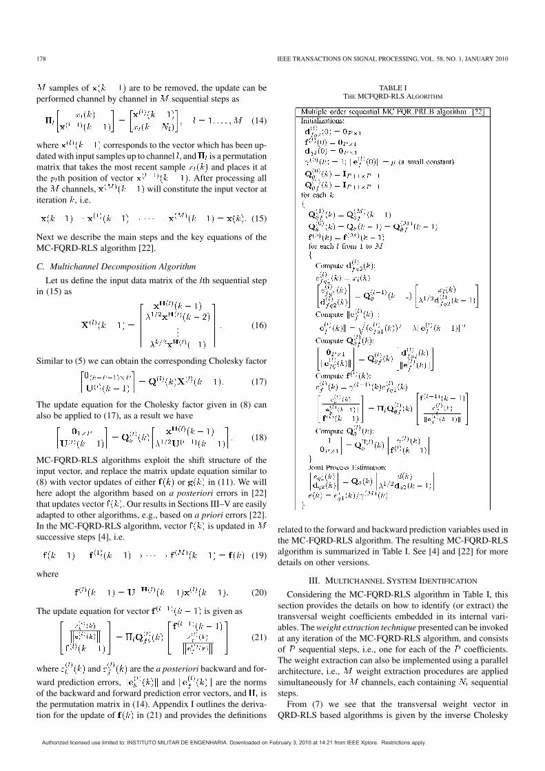
TABLE ITHE MCFQRD-RLS ALGORITHM

related to the forward and backward prediction variables used in

the MC-FQRD-RLS algorithm. The resulting MC-FQRD-RLS

algorithm is summarized in Table I. See [4] and [22] for more

details on other versions.

III. MULTICHANNEL SYSTEM IDENTIFICATION

Considering the MC-FQRD-RLS algorithm in Table I, this

section provides the details on how to identify (or extract) the

transversal weight coefficients embedded in its internal vari-

ables. The weight extraction technique presented can be invoked

at any iteration of the MC-FQRD-RLS algorithm, and consists

of sequential steps, i.e., one for each of the coefficients.

The weight extraction can also be implemented using a parallel

architecture, i.e., weight extraction procedures are applied

simultaneously for channels, each containing sequential

steps.

From (7) we see that the transversal weight vector in

QRD-RLS based algorithms is given by the inverse Cholesky



factor matrix and the rotated desired signal vector

. More specifically, each element, , of vector

is associated with one of the column vectors, , in

(22)

where the , are the index values corresponding to

in , see, e.g., Fig 1. This means that, when is given,

the elements of vector can be computed if all the columns

of the matrix are known. The two lemmas stated below

enable us to obtain all the column vectors in a serial

manner. The main result is that column vector can be

obtained from the column vector .

Lemma 1: Let be the column of

in (5) corresponding to coefficient of channel . Given

from Table I, then is ob-

tained from using

(23)

where , and

, and .

Lemma 2: Let be the column of

in (5) corresponding to coefficient of channel . Then

is obtained from in sequential steps

where step is given by

(24)

with and in

(21), and

for

for

otherwise.(25)

The recursion in (24), Appendix I-A, is performed to

, , and ,

and initialized with and

.

The proofs of Lemma 1 and Lemma 2 are provided in

Appendix II.

In order to extract the implicit weights associated with

each channel, Lemma 2 is initialized with , and, as

a result, we get column vector . Lemma 1 is then in-

voked to get the column vector . From we

can compute using Lemma 2. By induction we can con-

clude that all can be obtained. As a consequence, the ele-

ments of can be obtained from (22) in a serial manner. The

column extraction procedure is illustrated in Fig. 2 for the ex-

ample in Section II-B. The weight extraction algorithm is sum-

marized in Table II.

Fig. 2. The extraction of the first and second coefficient of channel 1.

TABLE IIWEIGHT EXTRACTION ALGORITHM

The computational complexity of the weight extraction is

given in Table IV.

Remark 1: From Table II it is noted that the weight extraction

algorithm can be applied to each channel simultaneously. Thus

the coefficients of each channel are extracted in sequential

steps, where . such parallel realizations allow

extraction of all the coefficients.

Remark 2: Using Lemma 1 and 2 the Cholesky factor

matrix corresponding to the initial conditions of the

MC-FQRD-RLS algorithm can be obtained and used in the



Fig. 3. Burst-trained adaptive filter setup. The adaptive filter is in training mode

for , and in data mode for ! . Note that there is no weight updateafter ! .

IQRD-RLS algorithm. This initialization renders precisely the

same learning curves for both algorithms.

Remark 3: The proposed method utilizes the internal vari-

ables with the aid of Givens rotation matrices to compute the

columns of . It is known, for the case of updating

backward prediction errors (resulting in lower triangular

Cholesky factor, as in the notation adopted in this paper) that

the rows of matrix are actually the coefficients of

the backward prediction filter of all orders (0 to ) [12]. The

weight extraction method based on computing the backward

prediction filter coefficients has been previously detailed in

[13]. This method uses the Levinson-Durbin recursions and

the alternative Kalman gain vector to extract the transversal

weight vector from the lattice coefficients which according to

[14] requires computations. Recently, another method

was presented in [15] that uses the Levinson-Durbin recursions

coupled with Cholesky factor update equation to extract the

transversal weights from the lattice coefficients.

IV. BURST-TRAINED EQUALIZERS

This section shows how to applyMC-FQRD-RLS algorithms

to problemswhere the filter coefficients are periodically updated

and then used for fixed filtering of a useful data sequence, e.g.,

burst-trained equalizers.

A. System Description

The problem under consideration is illustrated in Fig. 3.

As can be seen from the figure, the adaptive filter for time

instants is updated using its input and desired signal

pair ; we call it training mode. At time instant

, the adaptive process is stopped and from there onward

the coefficient vector at hand is frozen and used for

filtering; we call it data mode.

Such scenario can occur, for example, in periodic training

where the adaptive filter weights are not updated at every iter-

ation but after a certain data block. So, the adaptive filter acts

as an ordinary filter for the data block. As an example, consider

an equalizer design in a GSM environment, where the blocks of

training symbols are located within the data stream, and the es-

timation process is only carried out when training symbols are

encountered. The output of the filter is given by

(26)

TABLE IIIEQUIVALENT-OUTPUT FILTERING USING APPROACH 1 ALGORITHM

where is the coefficient vector of the adaptive filter

“frozen” at time instant . This approach of output

filtering is not realizable with the MC-FQRD-RLS algorithm.

If theMC-FQRD-RLS algorithm is employed during training,

one alternative for carrying out the filtering during data mode is

to first extract the filter coefficients according to Section III and,

thereafter, perform the filtering of with a simple transversal

structure. To avoid the increased peak complexity of this opera-

tion,wecan instead reuse thevariables from theMC-FQRD-RLS

update at time instant to reproduce the equivalent output

signal without the need of explicitly extracting the weights

, at . For the single channel FQRD-RLSalgorithm,

the equivalent output-filtering idea was presented in [17].

B. Approach I: Equivalent-Output Filtering Without Explicit

Weight Extraction

This section describes an output filtering method that does

not require explicit knowledge of the MC-FQRD-RLS weight

vector.

The variables from the MC-FQRD-RLS update at

can be reused to reproduce the equivalent-output signal associ-

ated with and . Using the definition of the weight

vector in (7), the filter output in data mode given by (26) can be

rewritten as

(27)



TABLE IVCOMPUTATIONAL COMPLEXITY OF WEIGHT EXTRACTION (WE), EQUIVALENT OUTPUT-FILTERING (EF) AND THE INDIRECT LEARNING MECHANISMS (IL)

where is explicitly available in the FQRD-RLS algo-

rithm at time instant . However, knowledge of

is only provided through the variable .

Thus, starting with as an initial value, we need to find a way

to obtain vector from vector ,

i.e., we need to incorporate the new sample without af-

fecting in the process. The solution exploits the fol-

lowing two relations:

(28)

Lemmas 3 and 4 summarize the steps required to compute (27)

without explicitly computing .

Lemma 3: Let denote the upper trian-

gular inverse Hermitian Cholesky matrix, and

denote the input data vector. Given

from Table I, then is obtained

from using the relation

(29)

where , and . The

proof for Lemma 3 is available in Appendix II.

Lemma 4: Given and

in (21), then

is obtained from in

sequential steps

where , and step is

given by

(30)

and

(31)

The proof for Lemma 4 is available in Appendix II. In order

to apply the above results for the filtering problem in Fig. 3,

we substitute with in Lemma 3

and 4 and set such that and

. Therefore starting from we

first obtain in sequential steps using Lemma 4

(32)

The updated vector is finally obtained from

in (32). The vector is then used in (27) to

produce . In order to get using Lemma 4 we first

need to compute by applying Lemma 3, i.e.

(33)

where . By induction, the output

for all values of can therefore be obtained with coef-

ficients of the MC-FQRD-RLS frozen at time instant . Note

that when is obtained from , only the input vector is

updated and matrix remains the same in the process.

The steps of the equivalent-output filtering algorithm and its

computational complexity are provided in Tables III and IV, re-

spectively.

C. Approach II: Equivalent-Output Filtering With Distributed

Weight Extraction

We can divide the input vector into two nonoverlapping

vectors and

(34)

with

(35)

where contains the input-samples from and

holds those remaining from . In other words, for each

time instant , the new input-samples are shifted into

and zeros are shifted into . This update process, which

is similar to (14), (15), is given by

(36)

with and .



The output for can now be written as

(37)

Note that with the initialization in (35), and

for .

The above formulation allows us to make use of our previous

results and divide the problem into two parts that can be car-

ried out in parallel: one equivalent-output part to produce

from the convolution of and the coefficients that are ob-

tained using weight extraction, and one equivalent-output part

reproducing .

Reproducing is straightforward. We only need to apply

the results in previous section using vector in place of

.

In order to compute the output for the coeffi-

cients of the channel are extracted using the parallel weight ex-

traction approach given as a remark in Section III. The weight

extraction gives one coefficient per channel per iteration. The

output is the sum of each channel output

(38)

We see from (38) that requires knowledge of

new weights (one per channel) per time instant , since

and for . We can thus

apply in parallel with the output filtering , an “on-the-fly”

weight extraction. The advantage of using parallel weight

extraction approach is that iterations are required to

extract all the weights, and then the output is simply given

by , where at , .

The computational complexity of this approach is given in

Table IV. For the initial operations the complexity is reduced

linearly from that of Approach 1. After all weights have been

acquired, the complexity is only multiplications per iteration

for the rest of the burst.

V. PREDITORTION OF HPA WITH MEMORY

This section shows how to apply the MC-FQRD-RLS algo-

rithm in an indirect-learning setup to linearize a nonlinear power

amplifier.

A. Problem Description

The objective of a predistorter is to linearize the nonlinear

transfer function (including memory) of a high-power ampli-

fier (HPA). As a result, more power efficient transmission is

allowed without causing signal waveform distortion and spec-

tral regrowth. Herein we consider an adaptive Volterra-based

predistorter that is designed using the indirect learning struc-

ture depicted in Fig. 4 [25]. This type of learning structure has

also been employed in several recently proposed predistorter de-

signs, see, e.g., [19] and [20]. In the indirect learning structure,

the predistorter coefficient vector is directly calculated

Fig. 4. Indirect learning based predistorter [25].

without the need for a PA parameter identification step. We see

in Fig. 4 that the predistorter coefficient vector is ob-

tained by minimizing the error signal obtained from the

training branch output signal and the predistorter output

signal . The parameters obtained in the training branch are

directly copied to the predistorter, avoiding the inverse calcula-

tion process.

Let us now consider an implementation where the

MC-FQRD-RLS algorithm is used for the predistorter identifi-

cation. We see from Fig. 4 that the coefficient vector embedded

in the MC-FQRD-RLS variables is needed for reproducing the

output signal , being the

predistorter input-signal vector. We know from Section III that

can be made explicitly available at every iteration.

However, as can seen from Table V such an approach will lead

to a solution of complexity per iteration. In other words,

there is no obvious gain of using an MC-FQRD-RLS algorithm

in place of an IQRD-RLS algorithm. One solution to this com-

plexity problem is to extract and copy the weights at a reduced

rate, say once every samples. Obviously, such an approach

will no longer yield identical results to an IQRD-RLS algorithm,

.and the convergence behavior will certainly be different

Our goal here is to reproduce, at each iteration, the exact

output associated with the weight vector em-

bedded in the MC-FQRD-RLS algorithm. The total computa-

tional complexity for calculating and updating

will be per iteration. The resulting structure will yield ex-

actly the same result as using an IQRD-RLS algorithm, while re-

ducing the computational complexity by an order of magnitude.

B. Multi-Channel Indirect Learning Predistorter

The solution is very similar to that of the problem dealt with

in Section IV where the weight vector in the MC-FQRD-RLS

algorithm was used for fixed filtering. The main difference here

is that the weight vector in the lower branch is continuously

updated by the MC-FQRD-RLS algorithm.

The output of the predistorter block is given by

(39)



where, and are parameters of the

MC-FQRD-RLS algorithm running in the lower branch of

Fig. 4. The rotated desired signal vector is directly

available in the MC-FQRD-RLS algorithm. However, the

Cholesky factor matrix is hidden in vector

. On the other hand, we

know from Lemma 4 that, given the new channel input

signals , matrix provides the relation

. Since vectors

and are both initially set to zero, we can modify (30) and

(31) for calculating for . The required computations

are summarized by Lemma 5.

Lemma 5: Let denote the product

, where is given in (5)

and is a multichannel input vector. Then

can be obtained from in sequential steps

where each step is given as

(40)

where

(41)

with and as in

(21). The index and, at

. Finally,

The proof of Lemma 5 is given in Appendix.

Equation (40) requires approximately multiplications at

each of the steps. Thus, the total number of multiplications

is . A better approximation of the computational com-

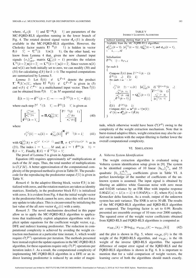
plexity of the proposedmethod is given in Table IV. The pseudo-

code for the reproducing the predistorter output is given in

Table V.

Remark 4: In the adaptive filtering block, vector is ini-

tializedwith zeros, and the rotationmatrices are taken as identity

matrices. Similarly, in the predistorter block is initialized

with zeros. It is evident from Fig. 4 that the initial weight vector

in the predistorter block cannot be zero, since this will not force

any update to take place. This is circumvented by initializing the

last value of the all zero vector with a unity.

Remark 5: The novel mechanisms described in this paper

allow us to apply the MC-FQRD-RLS algorithm to applica-

tions that traditionally exploit adaptation algorithms with ex-

plicit update equations for the coefficient weight vector, e.g.,

DFE and indirect learning predistorter. The reduction in com-

putational complexity is achieved by avoiding the weight ex-

traction mechanism at a particular time instant, , which would

require operations per iteration. The methods presented

here instead exploit the update equations in theMC-FQRD-RLS

algorithm, for these equations require only operations per

iteration index . As a result, the computational complexity of

implementing MC-FQRD-RLS algorithm in a DFE or an in-

direct learning predistorter is reduced by an order of magni-

TABLE VINDIRECT LEARNING ALGORITHM

tude, which otherwise would have been owing to the

complexity of the weight extraction mechanism. Note that in

burst-trained adaptive filters, weight extraction may also be car-

ried out in tandem with the output-filtering to further lower the

overall computational complexity.

VI. SIMULATIONS

A. Volterra System Identification

The weight extraction algorithm is evaluated using a

Volterra system identification setup given in [9]. The system

to be identified comprises of 10 linear and 55

quadratic coefficients given in Table VI. A

perfect knowledge of the number of coefficients of the un-

known system is assumed. The input signal is obtained by

filtering an additive white Gaussian noise with zero mean

and 0.0248 variance by an FIR filter with impulse response

, where is the

Kronecker delta function. As a result, output of the unknown

system has unit variance. The SNR is set to 30 dB. The results

of the MC-FQRD-RLS algorithm and IQRD-RLS algorithm

are compared. The forgetting factor is set to 0.99. Results

presented are ensemble average of 10 runs over 2000 samples.

The squared error of the weight vector coefficients obtained

from IQRD-RLS and FQRD-RLS algorithms is computed as

(42)

and the plot is shown in Fig. 5, where is the th

weight of the FQRD-RLS algorithm, and is the th

weight of the inverse QRD-RLS algorithm. The squared

difference of output error signal of the IQRD-RLS and the

FQRD-RLS algorithms is shown in Fig. 6. It is important to

mention that for a valid comparison of weight vectors, the

learning curve of both the algorithms should match exactly.



TABLE VILINEAR AND QUADRATIC COEFFICIENTS USED IN THE SYSTEM IDENTIFICATION SETUP

Fig. 5. Coefficient weight difference of the MC-FQRD-RLS algorithm and theIQRD-RLS algorithm.

Fig. 6. Difference in MSE of the MC-FQRD-RLS and the IQRD-RLS algo-rithms.

This means, both the algorithms should have equivalent initial

conditions. (See Remark 2 in Section III.)

Fig. 7. A decision feedback equalizer setup.

B. Burst-Trained DFE

In this section we consider a burst-trained decision feedback

equalizer (DFE), see Fig. 7. Viewing the DFE as a multichannel

filter we will have channels. In our simulations,

the lengths of feedforward and feedback filters

are and , respectively. A minimum phase

channel is considered, whose impulse response is defined

by .

During the first 300 iterations (i.e., ), the equalizer

coefficients are updated by the MC-FQRD-RLS algorithm.

The training symbols were randomly generated QPSK

symbols. Following the initial training sequence, an unknown

symbol sequence consisting of 700 16-QAM symbols was

transmitted over the channel and the equalizer output was

reproduced using the approach in Section IV. For comparison

purposes, an IQRD-RLS algorithm was also implemented.

Note that the IQRD-RLS has a complexity of during

coefficient adaptation. The SNR was set to 30 dB, and the

forgetting factor was chosen to . The training signal

was delayed by samples.

The learning curves, averaged over 50 ensembles, and the re-

covered constellation are shown in Figs. 8 and 9. The results

show that the MC-FQRD-RLS algorithm present exactly the

same behavior as IQRD-RLS algorithm.

C. Adaptive Volterra-Based Predistorter

The predistorter simulation setup for this example is taken

from [25], where a simplified baseband nonlinear satellite

channel is considered. The PA is modeled as a Wiener-Ham-

merstein system which is formed by a cascade of a linear filter

, a nonlinear function , and another linear filter . The



Fig. 8. Learning curves for the MC-FQRD-RLS algorithm using output fil-tering, and IQRD-RLS in DFE setup.

Fig. 9. 4-QAM constellation distorted by a linear channel and the equalizedconstellations using DFE implemented using the MC-FQRD-RLS (output fil-tering) and the IQRD-RLS algorithms.

non-linearity is due to the traveling wave tube amplifier (TWT)

with the AM/AM and AM/PM conversion given as

(43)

where , , , and are the constants given by 2.0, 1.0,

, and 1.0, respectively. The linear prefilter and postfilter re-

sponsible for the memory effects are taken as FIR with coeffi-

cient vectors

(44)

Fig. 10. Learning curve for the MC-FQRD-RLS algorithm using weight ex-traction Lemmas, and the IQRD-RLS algorithm.

Fig. 11. 16-QAM constellation distorted by a nonlinear amplifier and the com-pensated constellations using the indirect learning architecture.

A third-order Volterra model with a memory length of 7, i.e.,

119 taps is employed for the indirect learning architecture in

order to compensate for the nonlinear system. The input signal

comprises of 500 symbols from a 16-QAM constellation, and

there are 50 simulation runs. The maximum amplitude value

of the constellation is restricted to 0.64 so that the output of

the predistorter is in the input range of the nonlinear TWT

model. MC-FQRD-RLS algorithm with weight extraction is

compared with in-direct learning mechanism introduced in

Section V-B. Fig. 10 shows the same learning curve for both

algorithms. The IQRD-RLS algorithm is also considered for

comparison. It can be seen that all the learning curves converge

to 40 dB. The constellation diagram with and without a PD

is shown in Fig. 11. We see that both the IQRD-RLS and the

MC-FQRD-RLS algorithms are able to compensate for the

nonlinear distortion. However, the computational complexity

of the MC-FQRD-RLS algorithm is significantly lower than

that of the IQRD-RLS algorithm.



VII. CONCLUSIONS

This article showed how to reuse the internal variables of the

multichannel fast QR decomposition RLS (MC-FQRD-RLS)

algorithm to enable new applications which are different from

the standard output-error type applications. We first considered

the problem ofmultichannel (Volterra) system identification and

showed how to extract the weights in a serial manner. There-

after, the weight extraction results were extended to the case of

burst-trained decision-feedback equalizers, where the equalizer

is periodically retrained using pilots and then used for fixed fil-

tering of useful data. Finally, we considered the problem adap-

tive predistortion of high-power amplifiers using the indirect

learning control structure. Simulation results in these example

applications were compared with those using a designs based on

the inverse QRD-RLS algorithm. It was verified that identical

results are obtained using the FQRD-RLS methods at a much

lower computational cost.

APPENDIX I

A. Update of Vector

The forward and backward prediction and error vectors,

and for the th channel are defined as

(45)

(46)

where and are the respective forward and back-

ward prediction coefficient vectors, and and are

the forward and backward desired signal vectors given by

(47)

(48)

Let and de-

note the respective Givens rotations matrices responsible for the

Cholesky factorization of and , i.e.

(49)

and

(50)

The forward and backward prediction coefficient vectors that

minimize the norm of forward and backward prediction error

in (45) and (46), obtained in a similar manner as (7), are given

by

(51)

(52)

Equations (45) and (46) relate to each other via the permutation

matrix in (14) as [22]

(53)

From (53), we obtain

(54)

Inserting (49) and (50) in (54) yields

(55)

In order to relate the two square-root factors in (55) we need

to introduce the unitary transformation . Therefore,

we can write

(56)

where rotation matrix annihilates the

nonzero values and the permutation matrix operates from

left and right to shift rows and the columns to complete the tri-

angularization, see [22] for details. The norms and

are defined as

(57)

(58)

where and are the first elements of

and , respectively. They also related to vectors

and in similar way as relates to vector

in (9).

Inverting (56) and taking the Hermitian transpose results in

(59)



Note that the iteration index leads to the update from

to in -steps, where the current index value of th

channel input is consumed at each step. Finally, after post-

multiplying both sides of (59) with

we obtain

(60)

APPENDIX II

A. Proof of Lemma 1

The update equation for in the inverse QRD-RLS

algorithm is given by [16]

(61)

where . Premultiplying both

sides with and considering each column we get

(62)

where is the th element of vector

(63)

and and are provided by the

MC-FQRD-RLS algorithm.

B. Proof of Lemma 2

The proof follows directly from the column partitions of (59),

i.e.

(64)

where , , and

for

for

otherwise.

(65)We see from (59) that in order to obtain the first column, ini-

tialization has to be done with zeros. Therefore

and .

C. Proof of Lemma 3

Premultiply both sides of (61) with and post mul-

tiplying with the input signal vector leads to

(66)

where .

D. Proof of Lemma 4

We postmultiply (59) with a data vector

. This is allowed as

(59) can be postmultiplied by any input vector on both sides,

yielding Lemma 4.

E. Proof of Lemma 5

We postmultiply (59) with a data vector

. This is allowed as (59) can

be postmultiplied by any input vector on both sides, yielding

Lemma 5. Please note that the initially the input vector is set to

zero.

REFERENCES

[1] K. H. Kim and E. J. Powers, “Analysis of initialization and numericalinstability of fast RLS algorithms,” in Proc. Int. Conf. Acoust., Speech,Signal Process. (ICASSP’91), Toronto, Canada, Apr. 1991.

[2] P. A. Regalia and M. G. Bellanger, “On the duality between fast QRmethods and lattice methods in least squares adaptive filtering,” IEEETrans. Signal Process., vol. 39, no. 4, pp. 876–891, Apr. 1991.

[3] D. T. M. Slock, “Reconciling fast RLS lattice and QR algorithms,” inProc. Int. Conf. Acoust., Speech, Signal Process. (ICASSP’90), Albu-querque, NM, Apr. 1990, vol. 3, pp. 1591–1594.

[4] A. A. Rontogiannis and S. Theodoridis, “Multichannel fast QRD-LSadaptive filtering: New technique and algorithms,” IEEE Trans. SignalProcess., vol. 46, no. 11, pp. 2862–2876, Nov. 1998.

[5] A. Ramos, J. Apolinário, Jr., and M. G. Siqueira, “A new order recur-sive multiple order multichannel fast QRD algorithm,” in Proc. 38thAnn. Asilomar Conf. Signals, Syst., Comput., Pacific Grove, CA, Nov.2004.

[6] C. A. Medina, J. Apolinário, Jr., and M. Siqueira, “A unified frame-work for multichannel fast QRD-LS adaptive filters based on back-ward prediction errors,” inProc. IEEE Int. Midwest Symp. Circuits Syst.MWSCAS’O2, Tulsa, OK, Aug. 2002.

[7] J. A. Apolinário, Jr. and P. S. R. Diniz, “A new fast QR algorithmbased on a priori errors,” IEEE Signal Process. Lett., vol. 4, no. 11, pp.307–309, Nov. 1997.

[8] J. A. Apolinário, Jr., M. G. Siqueira, and P. S. R. Diniz, “Fast QR al-gorithms based on backward prediction errors: A new implementationand its finite precision performance,” Circuits Syst. Signal Process.,vol. 22, pp. 335–349, Jul./Aug. 2003.

[9] M. A. Syed and V. J. Mathews, “QR-decomposition based algorithmsfor adaptive Volterra filtering,” IEEE Trans. Circuits Syst. I: Fund.Theory Appl., vol. 40, no. 6, pp. 372–382, Jun. 1993.

[10] M. Shoaib, S. Werner, J. A. Apolinário, Jr., and T. I. Laakso, “Solutionto the weight extraction problem in FQRD-RLS algorithms,” in Proc.Int. Conf. Acoust., Speech, Signal Process. (ICASSP’06), Toulouse,France, May 2006.

[11] M. Shoaib, S. Werner, J. A. Apolinário, Jr., and T. I. Laakso, “Multi-channel fast QR-decomposition RLS algorithms with explicit weightextraction,” in Proc. EUSIPCO’2006, Florence, Italy, Sep. 2006.

[12] J. A. Apolinário Jr., QRD-RLS Adaptive Filtering. New York:Springer, 2009.

[13] S. Haykin, Adaptive Filter Theory, 3rd ed. Englewood Cliffs, NJ:Prentice-Hall, 1996.

[14] G. Carayannis, D. Manolakis, and N. Kalouptsidis, “A unified viewof parametric processing algorithms for prewindowed signals,” SignalProcess., vol. 10, no. 4, pp. 335–368, Jun. 1986.

[15] M. Shoaib, S. Werner, and J. A. Apolinário Jr., “Reduced complexitysolution for weight extraction in QRD-LSL algorithm,” IEEE SignalProcess. Lett., vol. 15, pp. 277–280, 2008.

[16] S. T. Alexander and A. L. Ghirnikar, “A method for recursive leastsquares filtering based upon an inverse QR decomposition,” IEEETrans. Signal Process., vol. 41, no. 1, pp. 20–30, Jan. 1993.

[17] M. Shoaib, S. Werner, J. A. Apolinário, Jr., and T. I. Laakso, “Equiv-alent output-filtering using fast QRD-RLS algorithm for burst-typetraining applications,” in Proc. ISCAS’2006, Kos, Greece, May 2006.

[18] D. Psaltis, A. Sideris, and A. A. Yamamura, “A multilayered neuralnetwork controller,” IEEE Control Syst. Mag., vol. 8, pp. 17–21, Apr.1988.



[19] D. R. Morgan, Z. Ma, J. Kim, M. G. Zierdt, and J. Pastalan, “Ageneralized memory polynomial model for digital predistortion of RFpower amplifiers,” IEEE Trans. Signal Process., vol. 54, no. 10, pp.3852–3860, Oct. 2006.

[20] L. Ding, G. T. Zhou, D. R. Morgan, Z. Ma, J. S. Kenney, J. Kim,and C. R. Giardina, “A robust digital baseband predistorter constructedusing memory polynomials,” IEEE Trans. Commun., vol. 52, no. 1, pp.159–165, Jan. 2004.

[21] M. Bouchard, “Numerically stable fast convergence least-squares algo-rithms for multichannel active sound cancellation systems and sounddeconvolution systems,” Signal Process., vol. 82, no. 5, pp. 721–736,May 2002.

[22] A. Ramos, J. A. Apolinário, Jr., and S. Werner, “Multichannel fastQRD-RLS adaptive filtering: Block-channel and sequential algorithmbased on updating backward prediction errors,” Signal Process., vol.87, pp. 1781–1798, Jul. 2007.

[23] A. Ramos and J. A. Apolinário, Jr., “A newmultiple order multichannelfast QRD algorithm and its application to non-linear system identifica-tion,” in Proc. XXI Simp. Brasileiro de Telecomun. SBT’04, Belém, PA,Brazil, Sep. 2004.

[24] P. S. R. Diniz, Adaptive Filtering: Algorithms and Practical Implemen-tation, 3rd ed. New York: Springer, 2008.

[25] C. Eun and E. J. Powers, “A new Volterra predistorter based on theindirect learning architecture,” IEEE Trans. Signal Process., vol. 45,no. 1, pp. 20–30, Jan. 1997.

Mobien Shoaib (M’03) received undergraduate ed-ucation in computer engineering from the NationalUniversity of Sciences and Technology (NUST)in 2001. He received the M.S. degree in telecom-munication engineering, from the Departmentof Electrical Engineering, Helsinki University ofTechnology (HUT), Espoo, Finland, in 2005.

He is working as a Researcher with the Depart-ment of Signal Processing and Acoustics, TKK.He is also currently associated with Prince SultanAdvanced Technology Research Institute (PSATRI),

King Saud University.

Stefan Werner (SM’04) received the M.Sc. degreein electrical engineering from the Royal Institute ofTechnology (KTH), Stockholm, Sweden, in 1998,and the D.Sc. (EE) degree (with honors) from theSignal Processing Laboratory, Smart and NovelRadios (SMARAD) Center of Excellence, HelsinkiUniversity of Technology (TKK), Espoo, Finland, in2002.

He is currently an Academy Research Fellow withthe Department of Signal Processing and Acoustics,TKK, where he is also appointed as a Docent. His re-

search interests include adaptive signal processing, signal processing for com-munications, and statistical signal processing.

Dr. Werner is a member of the editorial board for the Signal Processing

journal.

José Antonio Apolinário, Jr. (SM’04) graduatedfrom the Military Academy of Agulhas Negras(AMAN), Resende, Brazil, in 1981 and receivedthe B.Sc. degree from the Military Institute ofEngineering (IME), Rio de Janeiro, Brazil, in 1988,the M.Sc. degree from the University of Brasília(UnB), Brasília, Brazil, in 1993, and the D.Sc.degree from the Federal University of Rio de Janeiro(COPPE/UFRJ), Rio de Janeiro, in 1998, all inelectrical engineering.

He is currently an Adjunct Professor with the De-partment of Electrical Engineering, IME, where he has already served as theHead of Department and as the Vice-Rector for Study and Research. He wasa Visiting Professor with the Escuela Politécnica del Ejército (ESPE), Quito,Ecuador, from 1999 to 2000 and a Visiting Researcher and twice a Visiting Pro-fessor with Helsinki University of Technology (HUT), Finland, in 1997, 2004,and 2006, respectively. His research interests comprise many aspects of linearand nonlinear digital signal processing, including adaptive filtering, speech, andarray processing. He has recently edited the book QRD-RLS Adaptive Filtering

(New York: Springer, 2009).Dr. Apolinário has organized and been the first Chair of the Rio de Janeiro

Chapter of the IEEE Communications Society.


ieeetransactionsonsignalprocessing,vol.58,no.1,january2010...

Documents