ienac09te/ econometrics 1 final examination date: …leea.recherche.enac.fr/steve...

IENAC09TE/ Econometrics 1 Final Examination

Date: Wednesday 25 May 2011.

Time allowed: 2 hours (10:15-12:15).

Answer all questions brie�y.

Show all computations (including relevant critical values).

You are allowed all lecture handouts and notes, but no textbooks.

An English�French dictionary is allowed, as is a scienti�c calculator.

Question 1 is for 100 marks.

You are given a cross-sectional labour market dataset for 1499 U.S. individuals (in a given

year, which may be assumed to be 1993), adapted from the National Longitudinal Survey

of Youth (NLSY), which contains detailed information on wages, educational attainment

and ability, labour market experience, and family characteristics. The selected data is

for white males, each of whom worked for at least 30 weeks (800 hours) in the year,

and who earned between U.S.$1 and U.S.$100 per hour. The variables are LOGWAGE

(the natural logarithm of the hourly wage, measured in log U.S.$), EDUC (total years of

education), EXPER (years of work experience), ABILITY (score on a standard intelligence

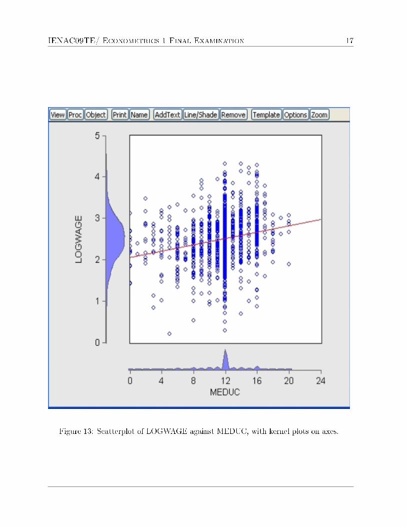
test), MEDUC (years of education received by the individual's mother), FEDUC (years of

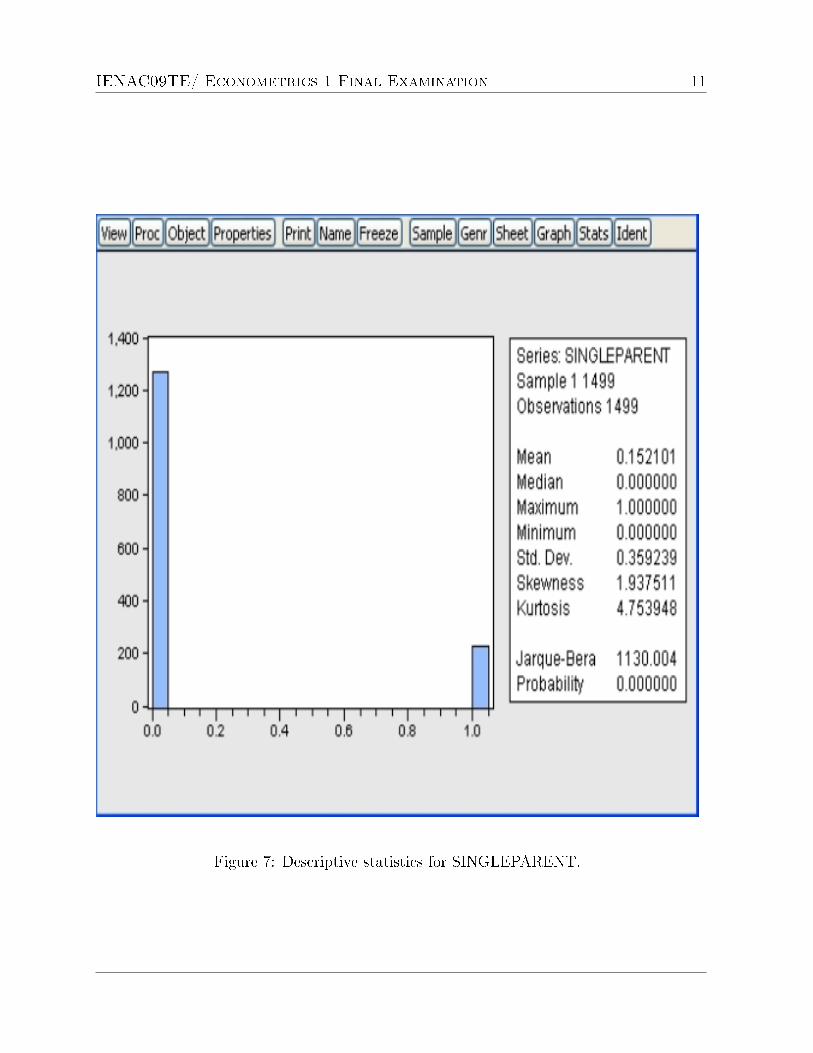
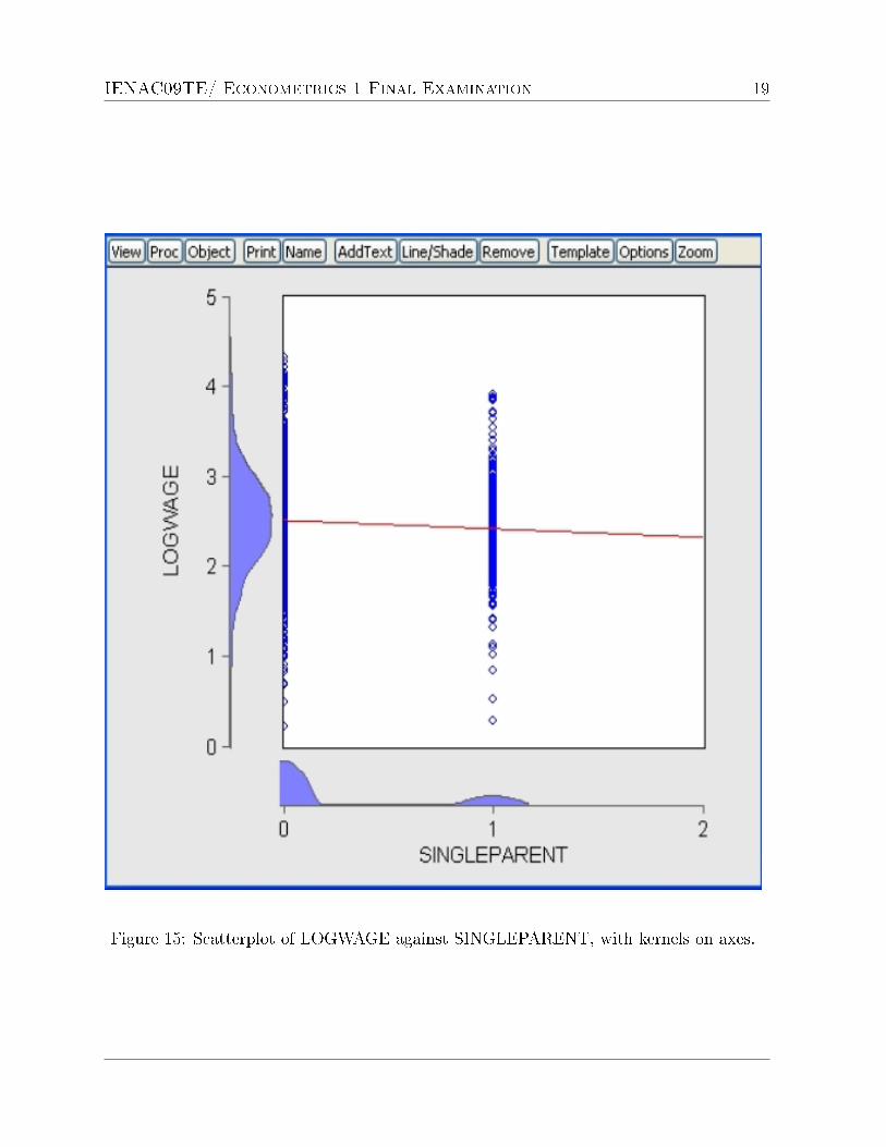
education received by the individual's father), SINGLEPARENT (dummy variable, taking

the value 1 if the individual's parents were separated / divorced, when the individual was 14

years old; and 0 otherwise), and SIBLINGS (number of brothers or sisters). Throughout,

log(·) refers to the natural logarithm; and (e.g.) “1.23E− 05” = 0.0000123.

This is used in Question 1.

IENAC09TE/ Econometrics 1 Final Examination 2

1 Question 1

• This question uses the labour market data (refer to Figures 1�42).

(a) Perform a careful �rst analysis of the variables, and explain your �ndings. Refer

to the descriptive statistics, bivariate correlations and scatterplots, and boxplots.

(15 marks)

(b) The following wage equation has been estimated using least squares (EQ01):

LOGWAGEi = β0 + β1EDUCi + β2EXPERi + β3ABILITYi

+ β4MEDUCi + β5FEDUCi + β6SINGLEPARENTi

+ β7SIBLINGSi + ui,

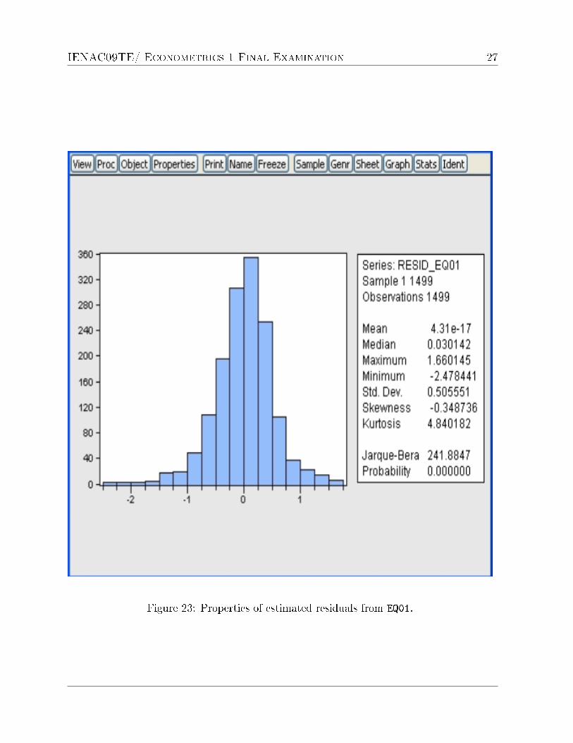
where i = 1, 2, . . . , n indexes the observation. Perform a careful assessment of the

regression output, and in particular the signi�cance of the variables, the signs and

magnitudes of the estimated coe�cients, and properties of the estimated residuals.

Which of the estimated coe�cients correspond to elasticities? (Interpret them.)

(15 marks)

(c) Test H0 : β2 = 0.02 against H1 : β2 > 0.02, at the 95% level, in EQ01. Interpret.

(8 marks)

(d) Test H0 : β4 = β5 = 0 against H1 : not H0, at the 99% level, in EQ01. Interpret.

(5 marks)


(e) The following wage equation has been estimated using least squares (EQ02):

LOGWAGEi = β0 + β1 log(EDUCi) + β2EXPERi + β3ABILITYi + β4MEDUCi

+ β5(log(EDUCi)× SINGLEPARENTi)

+ β6(EXPERi × SINGLEPARENTi)

+ β7(ABILITYi × SINGLEPARENTi)

+ β8(MEDUCi × SINGLEPARENTi) + ui.

Test whether the individual's education elasticity of wage is equal to 1, given that

SINGLEPARENTi is equal to 0 (then explain - without running an additional

test - how you would test the same hypothesis if SINGLEPARENTi equals 1).

(8 marks)

(f) In EQ02, what is the estimated percentage change in the hourly wage given a 2

point increase in ABILITY or an additional 5 years of EXPERIENCE?

(8 marks)

(g) The following wage equation has been estimated using least squares (EQ03):

LOGWAGEi = β0 + β1 log(EDUCi) + β2EXPERi + β3ABILITYi + β4MEDUCi

+ β5(ABILITYi × SINGLEPARENTi) + ui.

Interpret the results.

(8 marks)


(h) EQ04 is equivalent to EQ03, but with White's robust standard errors. What is

the impact of these on the regression results?

(3 marks)

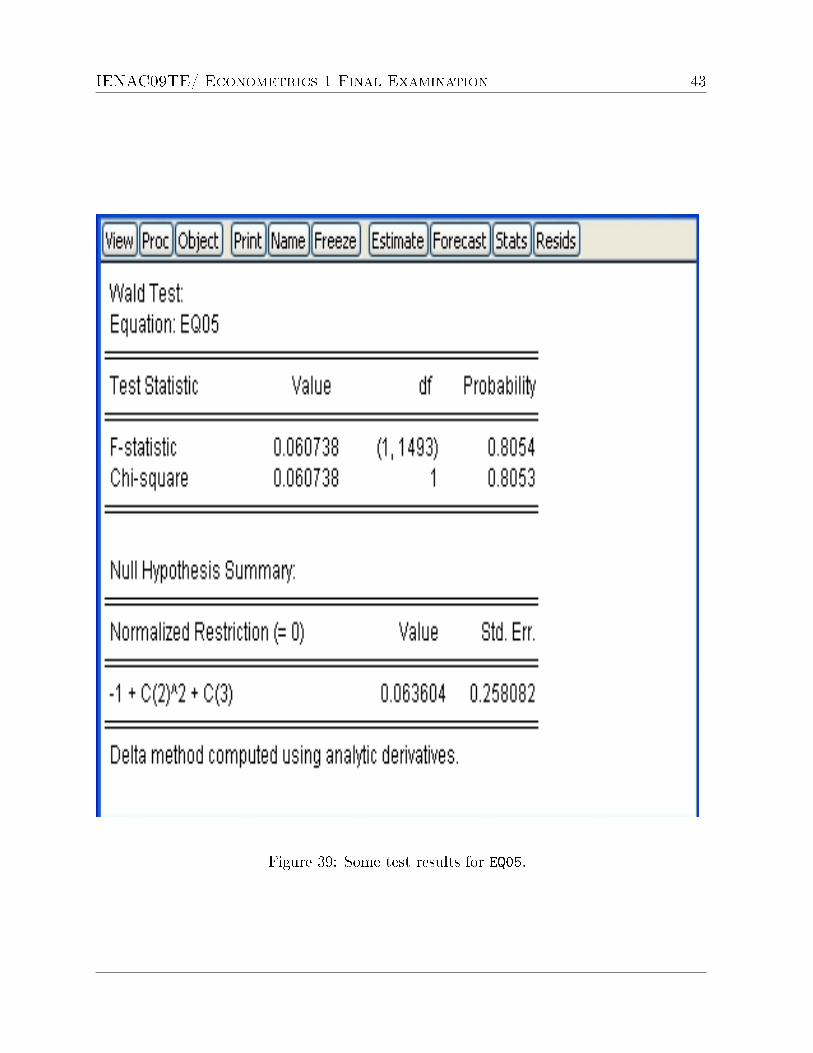
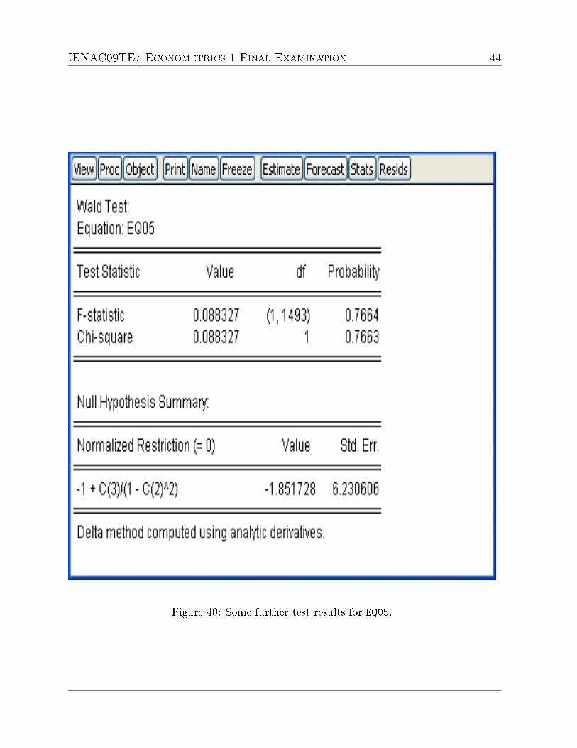
(i) EQ05 is equivalent to EQ03, but with Newey-West robust standard errors. Test

the hypotheses H0 : β21 + β2 = 1 and H0 : β2/(1− β2

1) = 1, both against their

two-sided alternatives, at the 95% level. What do you notice?!

(10 marks)

(j) EQ06 is equivalent to EQ03, but where the variable EXPER has been replaced by

EXPERα, and α is to be estimated. Test H0 : α = 1 against the two-sided

alternative, and carefully interpret.

(10 marks)

(k) Use EQ03 to forecast (estimate) the hourly wage of an individual with 18

years of education (highly-educated), 14 years of work experience (relatively little),

an ability test score of 2 (high ability), whose mother received 18 years of education

(also highly-educated), and who was not in a single-parent family at age 14

(parents not separated or divorced).

(10 marks)

(End of questions!)


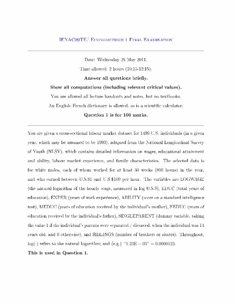
Figure 1: Descriptive statistics for LOGWAGE.


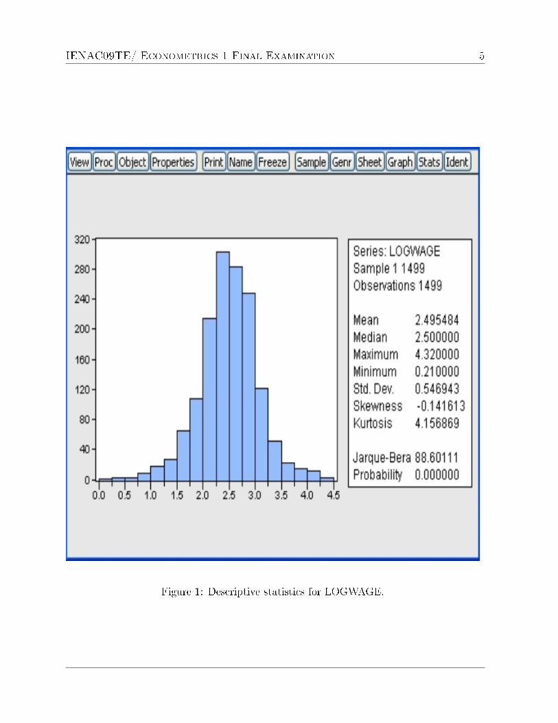
Figure 2: Descriptive statistics for EDUC.


Figure 3: Descriptive statistics for EXPER.


Figure 4: Descriptive statistics for ABILITY.


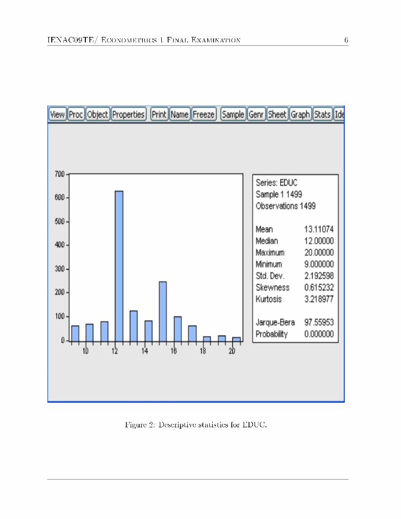
Figure 5: Descriptive statistics for MEDUC.


Figure 6: Descriptive statistics for FEDUC.


Figure 7: Descriptive statistics for SINGLEPARENT.


Figure 8: Descriptive statistics for SIBLINGS.


Figure 9: Bivariate correlations for variables.


Figure 10: Scatterplot of LOGWAGE against EDUC, with kernel plots on axes.


Figure 11: Scatterplot of LOGWAGE against EXPER, with kernel plots on axes.


Figure 12: Scatterplot of LOGWAGE against ABILITY, with kernel plots on axes.


Figure 13: Scatterplot of LOGWAGE against MEDUC, with kernel plots on axes.


Figure 14: Scatterplot of LOGWAGE against FEDUC, with kernel plots on axes.


Figure 15: Scatterplot of LOGWAGE against SINGLEPARENT, with kernels on axes.


Figure 16: Scatterplot of LOGWAGE against SIBLINGS, with kernel plots on axes.


Figure 17: Scatterplot of ABILITY against EDUC, with kernel plots on axes.


Figure 18: Scatterplot of EDUC against MEDUC, with kernel plots on axes.


Figure 19: Scatterplot of EDUC against FEDUC, with kernel plots on axes.


Figure 20: Scatterplot of EDUC against SIBLINGS, with kernel plots on axes.


Figure 21: Boxplots of variables.


Figure 22: EQ01 regression output.


Figure 23: Properties of estimated residuals from EQ01.


Figure 24: Scatterplot of estimated residuals from EQ01 against ABILITY.


Figure 25: Scatterplot of estimated residuals from EQ01 against SIBLINGS.


Figure 26: Estimated variance-covariance matrix from EQ01.


Figure 27: Some test results for EQ01.


Figure 34: Some further test results for EQ03.


Figure 40: Some further test results for EQ05.


Figure 43: Statistical table for N(0, 1). These tables have been taken from:http://fsweb.berry.edu/academic/education/vbissonnette/tables/tables.html.


Figure 44: Statistical table for Student's t(r).


Figure 45: Statistical table for F (m,n) at the 5% level.


Figure 46: Statistical table for F (m,n) at the 1% level.


Figure 47: Statistical table for χ2(q).

ienac09te/ econometrics 1 final examination date: …leea.recherche.enac.fr/steve...

Documents