ienac16 / econometrics 2 / applied problem set 2leea.recherche.enac.fr/steve...
TRANSCRIPT
IENAC16 / Econometrics 2 / Applied Problem Set 2
Topic: Heteroscedasticity
• This problem set deals with the detection of heteroscedasticity in cross-sectional data,
both visually and by use of several statistical diagnostic tests.
• We use data on monthly credit card expenditure, for n = 100 individuals, available
as credit_card.txt on the website.
• The variables are: Y1 (number of derogatory/negative reports), Y2 (indicator vari-
able: credit card application accepted? 1 = yes, 0 = no), X1 (age in years), X2
(0.0001 × income, in scaled U.S. dollars), X3 (average monthly credit card expendi-
ture, in U.S. dollars), X4 (indicator variable: individuals owns / rents home? 1 =
owns, 0 = rents), X5 (indicator variable: individual self-employed? 1 = yes, 0 = no).
• Refer to �gures 1 � 4, and perform the following:1
1. Perform a careful descriptive analysis of the dataset. In particular, (a) what
features of interest can you �nd for each of the variables?, (b) approximately
how many individuals have never had a credit card?! - look for evidence of
�rst-time applications, (c) consider bivariate scatterplots and correlations of Y2
against each of the other variables - interpret the signs of the correlations, and
(d) run a regression of Y2 on a constant, and all of the other variables - interpret
the signs and magnitudes of the estimated coe�cients, examine the signi�cance
of the variables, and compare your results with part (c) above.
1Note that not all of the necessary steps are shown in the �gures!

IENAC16 / Econometrics 2 / Applied Problem Set 2 2
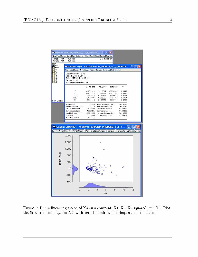
2. Run a linear regression of monthly expenditure on a constant, age, scaled in-
come, scaled income squared, and the home ownership indicator (eq01). Plot the
estimated residuals ui (resid_eq01) against scaled income, with kernel densities
superimposed on the axes (graph01), and interpret the results. Test manu-
ally for normality of the estimated residuals, and compare your result with the
EViews 6 (menu) version of the Jarque-Bera test. What do you notice?!
3. Perform White's nR2 general test for heteroscedasticity manually, at the 95%
level, where R2 is computed from the regression of the squared �tted residuals
u2i on a constant, all explanatory variables, and all squares and cross-products
of explanatory variables (eq02): explain why X42 is not included.
White's nR2 test is for the null H0 : σ2i = σ2 for all i = 1, 2, . . . , n, against
the alternative H1 : not H0. Interpret the results. Check your solution against
the EViews 6 (menu) version of this test.
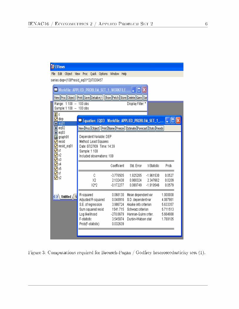
4. What is the estimated sum of squared residuals (u′u) from eq01? An alternative
test for heteroscedasticity is due to Breusch and Pagan, and Godfrey: it is a
Lagrange multiplier test of α = 0 (homoscedasticity) inH0 : σ2i = σ2f(α0+α′zi),
against H1 : not H0, where zi is some vector of variables excluding a constant.
The test statistic is:
BPGLM =1
2ESS =
1
2(y′y − ny2) ∼ χ2(m),
where ESS is the explained sum of squares from the regression of yi := nu2i /u′u
on a constant and zi, and m is the number of variables in (= dimension of) zi.
Use zi = (X2i,X22i )
′, and perform the test manually at the 95% level. Explain
carefully what you notice about the mean of y. Interpret your results. Check
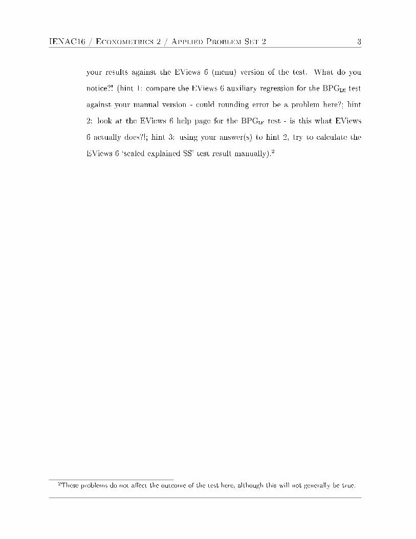
IENAC16 / Econometrics 2 / Applied Problem Set 2 3
your results against the EViews 6 (menu) version of the test. What do you
notice?! (hint 1: compare the EViews 6 auxiliary regression for the BPGLM test
against your manual version - could rounding error be a problem here?; hint
2: look at the EViews 6 help page for the BPGLM test - is this what EViews
6 actually does?!; hint 3: using your answer(s) to hint 2, try to calculate the
EViews 6 `scaled explained SS' test result manually).2
2These problems do not a�ect the outcome of the test here, although this will not generally be true.
IENAC16 / Econometrics 2 / Applied Problem Set 2 4
Figure 1: Run a linear regression of X3 on a constant, X1, X2, X2 squared, and X4. Plotthe �tted residuals against X2, with kernel densities superimposed on the axes.

IENAC16 / Econometrics 2 / Applied Problem Set 2 5
Figure 2: Auxiliary regression for White's nR2 general test for heteroscedasticity.
IENAC16 / Econometrics 2 / Applied Problem Set 2 6
Figure 3: Computations required for Breusch-Pagan / Godfrey heteroscedasticity test (1).

IENAC16 / Econometrics 2 / Applied Problem Set 2 7
Figure 4: Computations required for Breusch-Pagan / Godfrey heteroscedasticity test (2).
IENAC16 / Econometrics 2 / Applied Problem Set 2 8
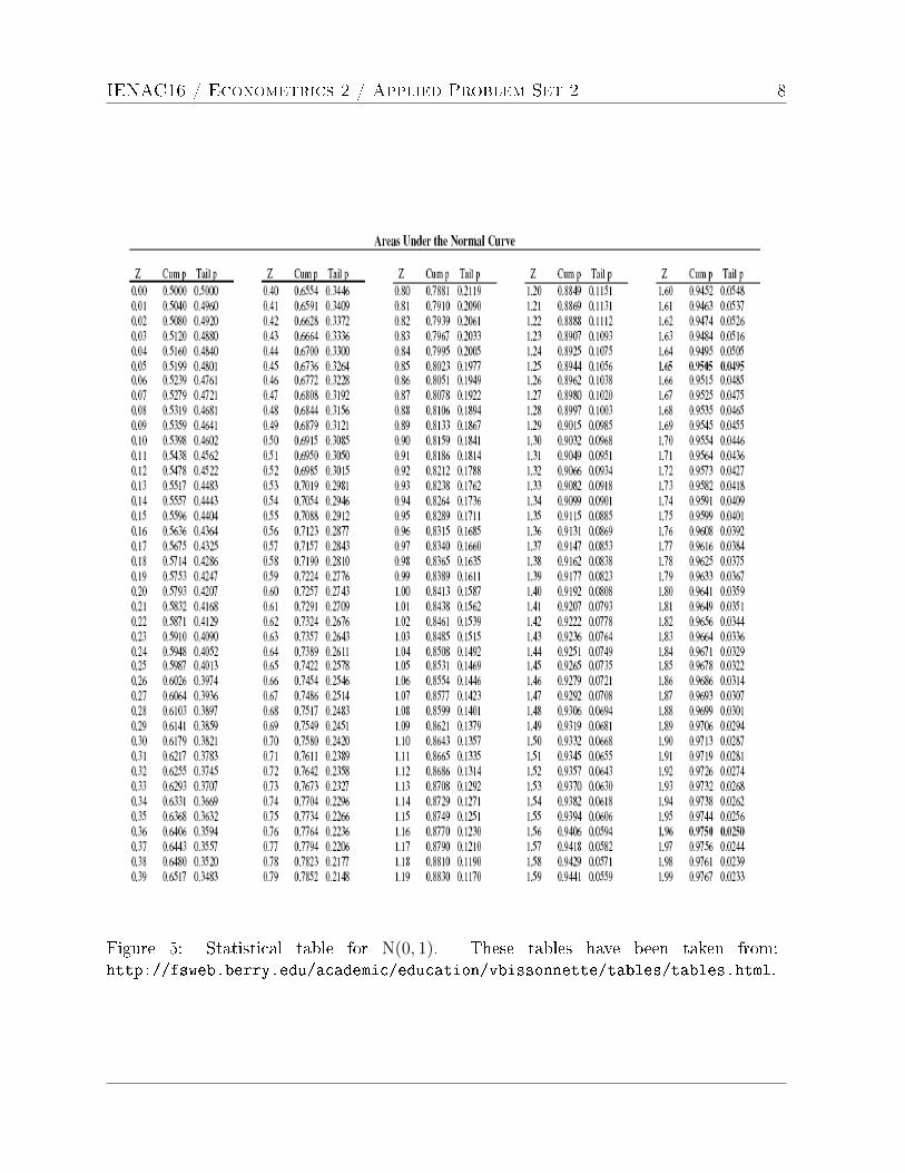
Figure 5: Statistical table for N(0, 1). These tables have been taken from:http://fsweb.berry.edu/academic/education/vbissonnette/tables/tables.html.

IENAC16 / Econometrics 2 / Applied Problem Set 2 9
Figure 6: Statistical table for Student's t(r).
IENAC16 / Econometrics 2 / Applied Problem Set 2 10
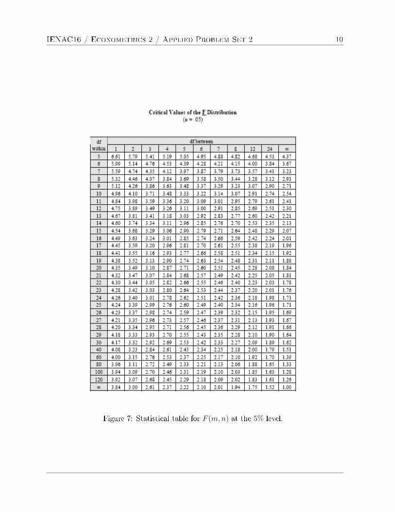
Figure 7: Statistical table for F (m,n) at the 5% level.

IENAC16 / Econometrics 2 / Applied Problem Set 2 11
Figure 8: Statistical table for F (m,n) at the 1% level.

IENAC16 / Econometrics 2 / Applied Problem Set 2 12
Figure 9: Statistical table for χ2(q).