Demand & Utility

What is Utility?

Satisfaction, happiness, benefit

Cardinal Utility vs. Ordinal Utility

Cardinal Utility: Assigning numerical values to the amount of satisfaction

Ordinal Utility: Not assigning numerical values to the amount of satisfaction but indicating the order of preferences, that is, what is preferred to what

Util

A unit of measure of utility

Total Utility

The amount of satisfaction obtained by consuming specified amounts of a product per period of time.

Example: TU(X) = U(X) = 16 X – X2

where X is the amount a good that is consumed in a given period of time.

5 units of the product per period of time yields 55 utils of satisfaction

Marginal Utility

The change in total utility (TU) resulting from a one unit change in consumption (X).MU = TU/ X

Diminishing Marginal Utility

Each additional unit of a product contributes less extra utility than the previous unit.

When the changes in consumption are infinitesimally small, marginal utility is the derivative of total utility.

MU = dTU/dX

Calculating MU from a TU FunctionExample: TU(X) = 16 X – X2

MU = dTU/dX = 16-2X

In general, the derivative of a total function is the marginal function.

The marginal function is the slope of the total function.

X

X

Total Utility

Marginal Utility

TU

MU

X1 X2

X1 X2

Graphs of Total Utility & Marginal Utility

X2 is where total utility reaches its maximum. MU is zero. This is the saturation point or satiation point.After that point, TU falls and MU is negative.

X1 is where marginal utility reaches its maximum. This is where we encounter diminishing marginal utility. The slope of TU has reached its maximum; TU has an inflection point here.

Example: If TU = 15 X + 7X2 – (1/3) X3, find (a) the MU function,

(b) the point of diminishing marginal utility, & (c) the satiation point.

a. MU = dTU/dX = 15 +14X – X2

b. Diminishing MU is where MU has a maximum, or the derivative of MU is zero.

0 = dMU/dx = 14 – 2X X = 7c. Satiation is where TU reaches a maximum or its

derivative (which is MU) is zero. How do we determine where MU = 15 +14X – X2 = 0 ?

Apply Quadratic Formula to –X2 + 14 X + 15 = 0 .

a2ac4bb

X2

)())(()(

1215141414 2

21614

152

30 X or 1

22

X either So

225614

Since a negative amount of a product makes no sense, X must equal 15.

If the previous example were about eating free cookies at a party, you’d eat 15 of them.

That is where you become satiated.After 15 cookies, you begin to feel a bit bloated.

When you have more than one product, the marginal utility is a partial derivative.

Calculating partial derivatives is no more difficult than calculating other derivatives. You just treat all variables as constants, except the one with which you are taking the derivative.We denote the partial derivative of Z with respect to X as Z/X instead of dZ/dX.

Example: Z = X2 +3XY + 5Y3

To take the partial derivative with respect to X, pretend Y is a constant (like 4). Then,

Z/X = 2X + 3Y .Similarly, to take the partial derivative with respect to Y, pretend X is a constant (like 4). So,

Z/Y = 3X + 15Y2 .

The Connection between Demand and Utility

Instead of thinking in terms of utils, let’s think in terms of dollars.

Suppose the purchase of one unit of a good gives you $10 worth of satisfaction.

In other words, the marginal utility of that first unit of the good is $10.

Then you would be willing to pay up to $10 for it.

If a second unit of the good contributes $8 more of satisfaction, the marginal utility of your second unit is $8 and you would be willing to pay up to $8 for it.

If a third unit of the good contributes $6 more of satisfaction, the marginal utility of your third unit is $6 and you would be willing to pay up to $6 for it.

Remember that the demand curve tells you what people are willing to pay for various amounts of a good or, equivalently, how many units of a good they are willing to purchase at various prices.

So, since we just found that the marginal utility tells us what we are willing to pay for a good, the marginal utility provides us with information that we can use to determine our demand curve.

In our example, we had the following:

Number of units purchased (Q)

Price you are willing to pay (P)

Marginal Utility

0 - -

1 10 10

2 8 8

3 6 6

If we graph that information, we get our demand curve.

Number of units purchased (Q)

Price you are willing to pay (P)

Marginal Utility

0 - -

1 10 10

2 8 8

3 6 6

price

quantity

10 8

6

1 2 3

Demand

Notice that by adding our MU values we can determine our total utility at different consumption levels.

Number of units purchased (Q)

Price you are willing to pay (P)

Marginal Utility

Total Utility

0 - - 0

1 10 10 10

2 8 8 18

3 6 6 24

Indifference Curve

A set of combinations of goods that are viewed as equally satisfactory by the consumer.

Indifference Map

A collection of indifference curves

Assumptions

1. The consumer can rank all bundles of commodities.

2. If bundle A is preferred to bundle B and B is preferred to C, then A is preferred to C. (This property is called transitivity.)

3. More is better.

Characteristics of indifference curves

Indifference curves slope down from left to right.Consider 2 points A & B on the same indifference curve. At point B, you have more food than at point A. If the amount of clothing you had at point B was the same as or more than at point A (like at point C), you would not be indifferent between A and B (since more is better).So A & B could not be on the same indifference curve, which goes against our initial statement that they are. So you must have less clothing at B, which means than B lies below A and the indifference curve slopes downward.

clothing

food

A

B

C

Indifference curves to the northeast are preferred.Point E is preferred to point A because it has more food & more clothing.Since you are indifferent between A & all points on IC1, E must be preferred to all points on IC1.Since you are indifferent between E and all points on IC2, all points on IC2 must be preferred to all points on IC1.

IC2

food

A

E

clothing

IC1

Indifference curves can not intersect.Suppose indifference curves could intersect. Let the intersection of IC1 & IC2 be D.Then you must be indifferent between D & any other point A on IC1.Similarly, you must be indifferent between D & any other point B on IC2.

food

A

D

clothing

IC1

B IC2

By transitivity, you must be indifferent between A & B.But A & B are not on the same indifference curve, which they should be if you are indifferent between them.Then, our initial supposition that indifference curves could intersect must be wrong.

Indifference curves are convex.[The curves become flatter as we move from left to right.]

When we have lots of clothing & not much food (as near A & B), we are willing to give up a lot of clothing to get a little more food.When we have lots of food & not much clothing (as near C & D), we are willing to give up very little clothing to get a little more food.

food

A

C

clothing

B

D

Odd special cases that are not consistent with the characteristics

listed previously.

Perfect Complements

You need exactly 4 tires with 1 car body (ignoring the spare tire).

Having more than 4 tires with 1 car body doesn’t increase utility.

Also having more than 1 car body with only 4 tires doesn’t increase utility either.

tires

Car bodies1 2

8

4IC1

IC2

Perfect Substitutes

Consider two packs of paper; the mini-pack has 100 sheets & the jumbo pack has 500 sheets.No matter how many mini-packs or jumbo packs you have, you are always willing to trade 5 mini-packs for 1 jumbo pack.Since the rate at which you’re willing to trade is the slope of the IC, and that rate is constant, your IC’s have a constant slope.That means they are straight lines.

Mini-packs

Jumbo packs

1 2

10

5

IC1

IC2

Goods versus Bads

As you get more of a bad, you need more of a good to compensate you, to keep you feeling equally happy.So IC of a good & a bad slopes upward.

production

pollution

IC1

IC2

“Neutral” Good

Your utility is unaffected by consumption of a neutral good.

Neutral good

Desired good

IC1 IC2 IC3

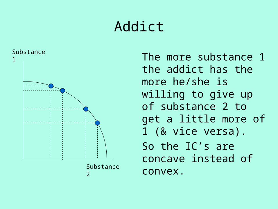
Addict

The more substance 1 the addict has the more he/she is willing to give up of substance 2 to get a little more of 1 (& vice versa).So the IC’s are concave instead of convex.

Substance 1

Substance 2

The slope of the indifference curve is the rate at which you are willing to trade off one good to get another good.

It is called the marginal rate of substitution or MRS.

What is the MRS or slope of the IC? Suppose points A & B are on the same indifference curve & therefore have the same utility level. Let’s break up the move from A to B into 2 parts.AD: TU = C (MUC)DB: TU = F (MUF)AB: 0 = TU = C (MUC) + F (MUF) C (MUC) = – F (MUF) C/F = – MUF / MUC

IC1

Food F

A

D

Clothing C

B

IC2

So along an indifference curve, the slope or MRS is the negative of the ratio of the marginal utilities (with the MU of the good on the horizontal axis in the numerator).

MRS = – MUX / MUY

For example,Suppose IC1 is the 90-util indifference curve & IC2 is the 96-util indifference curve. Point A is 7 units of food & 6 of clothing. B is 9 units of food & 5 of clothing.Since an additional unit of clothing gives you 6 more utils of satisfaction, the MU of clothing must be 6.Since an additional 2 units of food also give you 6 more utils of satisfaction, the MU of food must be 3. So, MRS = – MUF / MUC = -3/6 = -0.5 .You’d give up 2 units of food to get 1 units of clothing.

IC1 =90

Food F

A

D

Clothing C

B

IC2 = 96

6

5

7 9

Budget Constraint or Budget Line

This equation tells you what you can buy.For example, suppose you have $24, & there are

two goods. The price of the first good is $3 per unit & the price

of the second good is $4 per unit. So, if you buy X units of the first good for $3 each,

you spend 3X on that good.Similarly, if you buy Y units of the second good, you

spend 4Y on that good.Your total spending is 3X+4Y.If you spend all 24 dollars that you have, 3X+4Y=24.That equation is your budget constraint.

Example: Budget constraint for $24 of income, and $3 & $4 for the prices of the two goods.

X

Y

(0,6)

(8,0)0

If you spent all $24 on the 1st good, you could buy 8 units.If you spent all $24 on the 2nd good, you could buy 6 units.So we have the intercepts of the budget constraint. The slope of the line connecting these two points is Y/X = – 6/8 = – 3/4 = – 0.75 .

Let’s generalize. Keep in mind that income was $24 and the prices of the goods were $3 & $4. The equation of the budget constraint in our example was 3X + 4Y = 24.

X

Y

(0,6)

(8,0)0

So the budget constraint is p1X + p2Y = I Solving for Y in terms of X, p2Y = I – p1X,

or Y = I /p2 – (p1/p2)X

So from our slope-intercept form, we see that the intercept is I /p2, and the slope is –p1/p2 .

The intercept is income divided by the price of the good on the vertical axis. The slope is the negative of the ratio of the prices, with the price of the good on the horizontal axis in the numerator.

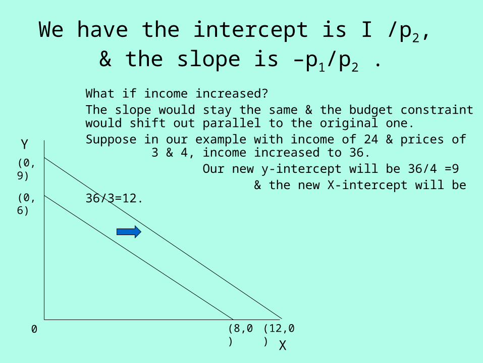
We have the intercept is I /p2, & the slope is –p1/p2 .

What if income increased? The slope would stay the same & the budget constraint would shift out parallel to the original one.Suppose in our example with income of 24 & prices of 3 & 4, income increased to 36. Our new y-intercept will be 36/4 =9 & the new X-intercept will be 36/3=12.

X

Y

(0,6)

(8,0)0

(0,9)

(12,0)

Suppose the price of the good on the X-axis increased.If we bought only the good whose price increased, we could afford less of it. If we bought only the other good, our purchases would be unchanged. So the budget constraint would pivot inward about the Y-intercept.

X

Y

(0,6)

(8,0)0 (6,0)

For example, if the price increased from $3 to $4, our $24 would only buy 6 units.

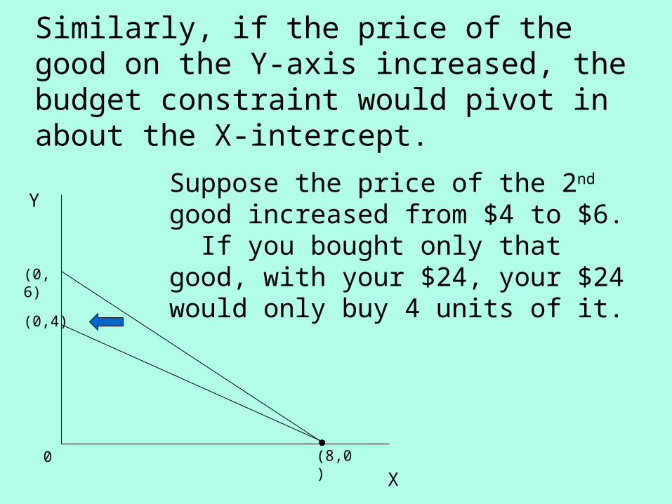
Similarly, if the price of the good on the Y-axis increased, the budget constraint would pivot in about the X-intercept.

X

Y

(0,6)

(8,0)0

(0,4)

Suppose the price of the 2nd good increased from $4 to $6. If you bought only that good, with your $24, your $24 would only buy 4 units of it.

Let’s combine our indifference curves & budget constraint to determine our utility maximizing point.

Point A doesn’t maximize our utility & it doesn’t spend all our income. (It’s below the budget constraint.)

X

Y

0

IC1

IC2

IC3

A

Points B & C spend all our income but they don’t maximize our utility. We can reach a higher indifference curve.

X

Y

0

IC1

IC2

IC3

B

C

Point D is unattainable. We can’t reach it with our budget.

X

Y

0

IC1

IC2

IC3

D

Point E is our utility-maximizing point.We can’t do any better than at E.Notice that our utility is maximized at the point of tangency between the budget constraint & the indifference curve.

X

Y

0

IC1

IC2

IC3

E

Recall from Principles of Microeconomics, to maximize your utility, you should purchase goods so that the marginal utility per dollar is the same for all goods.

If there were just two goods, that means that MU1/P1 = MU2/P2

Multiplying both sides by P1/MU2, we have MU1/MU2 = P1/P2 .The expression on the right is the negative of the slope of the

budget constraint.The expression on the left is the negative of the slope of the

indifference curve.So the slope of the indifference curve must be equal to the slope

of the budget constraint.If at a particular point, two functions have the same slope, they

are tangent to each other.That means your utility-maximizing consumption levels are where

your indifference curve is tangent to the budget constraint.This is the same conclusion we reached using our graph.

Example: If TU = 10X + 24Y – 0.5 X2 – 0.5 Y2, the prices of the two goods are 2 and 6, and we have

$44, how much should you consume of each good?

Taking the derivatives of TU we haveMU1 = 10 – X and MU2 = 24 – Y

Since MU1/MU2 = P1/P2 , we have(10 – X) / (24 – Y) = 2 / 6 ,

or 60 – 6 X = 48 – 2Y , or 6X – 2Y = 12 .This an equation with two unknowns.Our budget constraint provides us with a 2nd equation.

Combining the two equations, we can solve for X & Y.The budget constraint is 2X + 6Y = 44 .

So our two equations are 6X – 2Y = 12 and 2X + 6Y = 44

Multiplying the second equation by 3 yields6X + 18Y = 132 .

Now we have 6X + 18Y = 132 6X – 2Y = 12 --------------------

So, 20Y = 120and Y = 6 .Plugging 6 in for Y in the 1st equation yields 6X – 12 = 12,or 6X = 24. So, X = 4 .

Let’s see if all this works.We had $44, the prices were 2 & 6, and MU1 = 10 – X & MU2 = 24 – Y. We bought 4 units of the 1st good & 6 of the 2nd good.First, did we spend exactly what we had?We spent (2)(4) + (6)(6) = 8 + 36 = 44 Good.Is the marginal utility per dollar the same for both goods?

For the 1st good: MU1/P1 = (10 – X)/2 = (10-4)/2 = 3

For the 2nd good: MU2/P2 = (24 – Y)/6 = (24-6)/6 = 3

So they’re equal and things look fine.

What happens to consumption when income rises?

For normal goods, consumption increases.For inferior goods, consumption decreases.What does this look like on our graph?

Two Normal GoodsAs income increases, the budget constraint shifts out & we are able to reach higher & higher IC’s.The points of tangency are at higher & higher levels of consumption of both goods.

X

Y

IC1

IC2

IC3

C

B

A

Y3

Y2

Y1

X1 X2 X3

Income-Consumption CurveThe curve that traces out these points is called the income-consumption curve.For two normal goods, the curve slopes upward.It may be convex (as drawn here), concave, or linear.

X

Y

IC1

IC2

IC3

C

B

A

Y3

Y2

Y1

X1 X2 X3

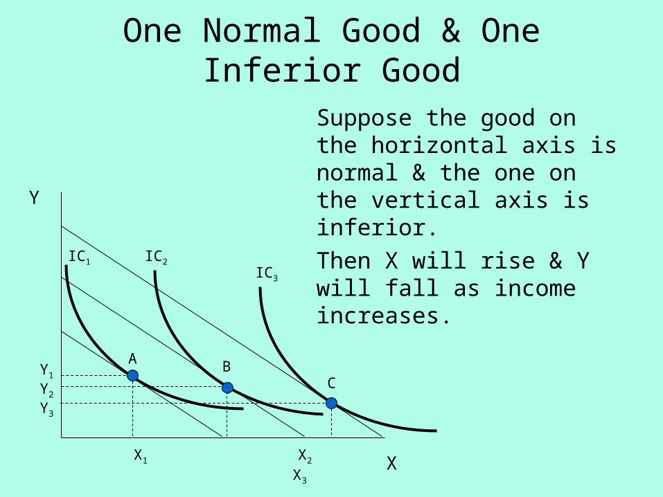
One Normal Good & One Inferior Good

Suppose the good on the horizontal axis is normal & the one on the vertical axis is inferior. Then X will rise & Y will fall as income increases.

X

Y

IC1 IC2IC3

CBA

X1 X2 X3

Y1

Y2

Y3

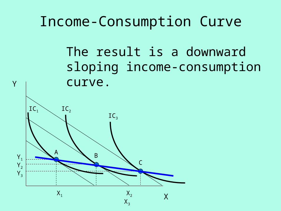
Income-Consumption Curve

The result is a downward sloping income-consumption curve.

X

Y

IC1 IC2IC3

CBA

X1 X2 X3

Y1

Y2

Y3

Engel CurveThe Engel Curve shows the quantity of a good purchased at each income level.The graph has income on the vertical axis and the quantity of the good on the horizontal.It slopes up for normal goods & down for inferior goods.X

Income

C

B

A

X1 X2 X3

I3

I2

I1

We can also look at consumption levels of two goods when the price of one of them changes.

Suppose there is an increase in the price of the 1st good (the good on the X-axis).The budget constraint pivots inward. Here we see X drop & Y increase. In this case, our 2 goods are substitutes.

X

Y

X3 X2 X1

Y3

Y2

Y1

If we connect the points, we have the price consumption curve.

It shows the utility-maximizing points when the price of a good changes.

X

Y

X3 X2 X1

Y3

Y2

Y1

If we look at the price of a good & the amount of it consumed, we have the demand curve

for our particular individual.

As the price decreases the quantity demanded increases & vice versa.

X

P

X1 X2 X3

P1

P2

P3

We can separate the effect of a change in the price of a good on its consumption level into two parts: the income effect & the substitution effect.

Suppose the price of the first good increases.The budget constraint was originally the blue line and we were at A consuming quantities XA & YA. After the price change, the budget constraint is the red line, and we’re at B consuming XB & YB .

X

Y

ABYB

YA

XB XA

We first want to capture the effect of the price change without the effect of the change in income.

X

Y

H

ABYH

YB

YA

XB XH XA

We draw a line parallel to the new budget constraint and tangent to the old indifference curve.This will reflect the new relative prices, but since we are tangent to the old indifference curve we are just as well off as initially. Under those circumstances we would be at point H (for hypothetical).Since the 1st good is now relatively more expensive compared to the 2nd, we will substitute, increasing Y & decreasing X.

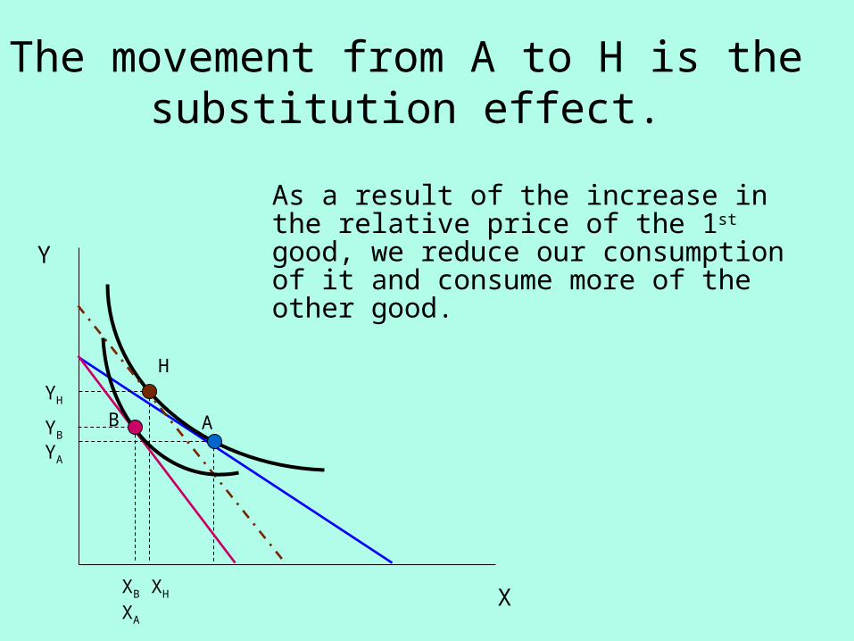
The movement from A to H is the substitution effect.

X

Y

H

ABYH

YB

YA

XB XH XA

As a result of the increase in the relative price of the 1st good, we reduce our consumption of it and consume more of the other good.

Now we move from H to B

XX

Y

H

ABYH

YB

YA

XB XH XA

Our purchasing power has been reduced by the price change. That results in the income effect.In our graph, we now hold the relative prices constant at the new level, but income has fallen. Our budget constraint has shifted inward. If both goods are normal, as a result of the change in income, we reduce our consumption of both goods, and X & Y fall.This is the income effect of the price change.

Total Effect of Price Increase

X

Y

H

ABYH

YB

YA

XB XH XA

The total effect is to move from A to B.X has fallen.Both the substitution & income effects led to a drop in X.Y has increased in this case.The substitution effect increased consumption of the 2nd good, but the income effect reduced it by less than the substitution effect increased it.

Let’s do a price decrease.

X

Y

H

B

A

YB

YA

YH

XA XH XB

The budget constraint moves from the blue line to the red line.We draw a line parallel to the new budget constraint and tangent to the old indifference curve.H is the tangency of the hypothetical budget constraint with the old indifference curve.The substitution effect is the movement from A to H. We substitute increasing X & decreasing Y.

The movement from H to B is the income effect.

X

Y

H

B

A

YB

YA

YH

As a result of the higher income (greater purchasing power), we consume more of both goods, if they are normal goods.

XA XH XB

Total Effect

X

Y

H

B

A

YB

YA

YH

The total effect is to move from A to B.X has increased.Both the substitution & income effects led to an increase in X.Y has also increased in this case.The substitution effect decreased consumption of the 2nd good, but the income effect increased it by more than the substitution effect decreased it.

XA XH XB

Income and Substitution Effects, in words

The income effect is the result of the change in purchasing power.

If the price of a normal good increases, you feel poorer, and the income effect is to consume less.

If the price of a normal good decreases, you feel richer, and the income effect is to consume more.

The substitution effect is the result of a change in relative prices.

If the price of a good increases, the substitution effect is to consume less of it & more of the other goods that are now relatively cheaper.

If the price decreases, the substitution effect is to consume more of it & less of the goods that are now relatively more expensive.

What if the price changed of an inferior good?

The substitution effect would be the same but the income effect would be the opposite.

Price increase for an inferior goodIncome effect: Your purchasing power has decreased. You feel poorer.

So you consume more of the inferior good.

Substitution effect:The good is now relatively more expensive than other goods,

so you consume less of it and more of other goods.

Notice the IE & SE are in opposite directions in this case.If the SE is larger than the IE, you will consume less of the

good.If the IE is larger than the SE, you will consume more of the

good.

An inferior good for which the IE is larger than the SE is called a Giffen good.

It is a good for which consumption rises when the price increases, and consumption falls when the price decreases.

Price decrease for an inferior goodIncome effect: Your purchasing power has increased. You feel richer. So

you consume less of the inferior good.Substitution effect:The good is now relatively more cheaper than other goods,

so you consume more of it and less of other goods.Again the IE & SE are in opposite directions in this case.If the SE is larger than the IE, you will consume more of the

good.If the IE is larger than the SE, you will consume less of the

good.

We previously looked at the demand curve for individuals. How do we get the market demand curve from the demand curve for individuals? We just horizontally sum up the individual demand curves.

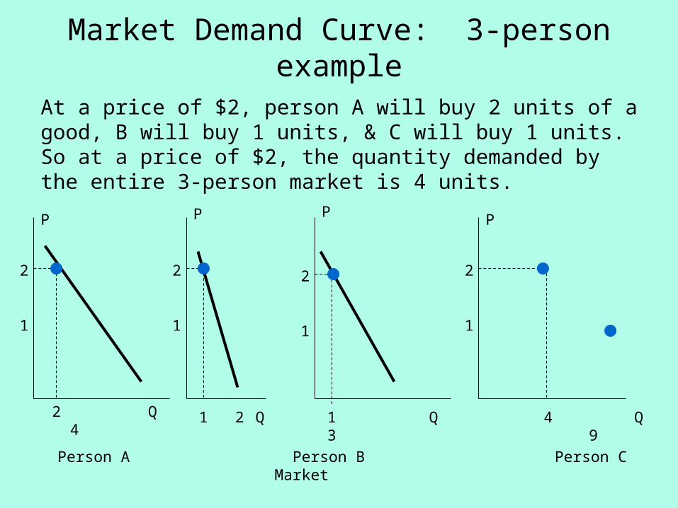
Market Demand Curve: 3-person example

Person A Person B Person C Market

P P

Q Q

2

1

2

1

2 4

P P

Q Q

2

1

2

1

4 91 31 2

At a price of $1, person A will buy 4 units of a good, B will buy 2 units, & C will buy 3 units. So at a price of $1, the quantity demanded by the entire 3-person market is 9 units.

Market Demand Curve: 3-person example

Person A Person B Person C Market

P P

Q Q

2

1

2

1

2 4

P P

Q Q

2

1

2

1

4 91 31 2

At a price of $2, person A will buy 2 units of a good, B will buy 1 units, & C will buy 1 units. So at a price of $2, the quantity demanded by the entire 3-person market is 4 units.

Market Demand Curve: 3-person example

Person A Person B Person C Market

P P

Q Q

2

1

2

1

2 4

P P

Q Q

2

1

2

1

4 91 31 2

Continuing the process, we get the market demand curve.

The Demand for a product can be expressed as a function of

1. its price (changes in which lead to movements along the demand curve), and

2. other determinants such as income, prices of related goods, & expectations (changes in which lead to shifts of the demand curve).

So we have QDX = g(PX, Psubst, Pcomp, Inc., Expect.) A particular demand curve QDX = g(PX) shows the

relation between the quantity demanded of a product and its price when we hold all the factors constant. This is also sometimes written as P= f(Q).

TR = PQ

Total Revenue

Average Revenue

total revenue per unit of output

AR = TR / Q = (PQ) / Q

= P

AR & P are the same function of Q.

Marginal Revenue

The additional revenue associated with an additional unit of output

MR = dTR / dQ

Example: Horizontal Demand Curve(price is a constant function)

P

Q

10D

Q

PTRslope = MR = 10

= AR =MR

P = f(Q) = 10

AR = P = 10TR = PQ = 10 Q

MR = dTR / dQ = 10

So D, AR, & MR are the same horizontal function.

TR is an upward sloping line with a constant slope.

Implications for revenue:Every time you sell another unit of output, revenue increases by the

price, which is constant.

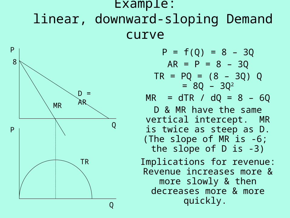
Example: linear, downward-sloping Demand curve

P

Q

8

D = AR

Q

P

TR

MR

P = f(Q) = 8 – 3QAR = P = 8 – 3Q

TR = PQ = (8 – 3Q) Q= 8Q – 3Q2

MR = dTR / dQ = 8 – 6QD & MR have the same vertical intercept. MR is twice as steep as D. (The slope of MR is -6;

the slope of D is -3)Implications for revenue:

Revenue increases more & more slowly & then decreases

more & more quickly.

Example:quadratic, downward-sloping Demand curve

P

Q

20D = AR

Q

P

TR

MR

P = f(Q) = 20 – Q2

AR = P = 20 – Q2

TR = PQ = (20 – Q2) Q= 20Q – Q3

MR = dTR / dQ = 20 – 3Q2

MR is a quadratic; TR is a cubic.

Elasticity

Responsiveness or sensitivity of one variable to a change in another variable

(% change in X)ε = ------------------------ (% change in Y)

Price Elasticity of Demand

(% change in quantity demanded)ε = ------------------------------------------------ (% change in price)

Two methods of calculating elasticity

Arc elasticity: measures responsiveness between 2 points

Point elasticity: measures responsiveness at a single point for an infinitesimally small change

Arc Elasticity

ΔQ/(avg Q) [Q2 – Q1] / [(Q1+Q2)/2]--------------- = --------------------------------ΔP/(avg P) [P2 – P1] / [(P1+P2)/2]

Arc Elasticity ExampleCalculate the price elasticity of demand if in response to a increase in

price from 9 to 11 dollars, the quantity demanded decreases from 60 to 40 units.

P: 9→11 Q: 60→40

ΔQ/(avg Q) [Q2 – Q1] / [(Q1+Q2)/2]ε = --------------- = -------------------------------- ΔP/(avg P) [P2 – P1] / [(P1+P2)/2]

[40 – 60] / [(60+40)/2] -20 / 50 -0.4 = ------------------------------ = ------------ = ------- = -2.0 [11 – 9] / [(9+11)/2] 2 / 10 0.2

The negative sign indicates that price & quantity move in opposite directions.

The negative sign is sometimes dropped with the understanding that price & quantity are still moving in opposite directions.

Point Elasticity

dQ / Q dQ Pε = ---------- = ----- ---- dP / P dP Q

Point Elasticity Example

If the demand function is Q = 245 – 3.5 P, find the price elasticity of demand when the price is 10.

When P = 10, Q = 245 – 3.5(10) = 210

The derivative dQ / dP = = – 3.5

dQ / Q dQ P 10ε = ---------- = ----- --- = - 3.5 ------ = - 0.167 dP / P dP Q 210

Categories of Price Elasticity of Demand

Demand is elastic if |ε| > 1Demand is inelastic if |ε| < 1Demand is unit elastic if |ε| = 1

What is the relationship between elasticity & the slope of the demand curve?

dQ / Q dQ P 1 Pε = ---------- = ----- ---- = -------- ---- dP / P dP Q dP/dQ Q

= (1/slope) (P/Q)

So, if 2 demand curves pass through the same point (& therefore have the same values of P & Q at that point), the flatter curve (curve with the smaller slope) has the greater elasticity at that point.

Example

At point E, D1 has greater elasticity than D2 .

P

Q

E

D2

D1

Elasticity on a Linear Demand Curve

At the midpoint, |ε| = 1 (unit elasticity)

Above the midpoint, |ε| > 1 (elastic)

Below the midpoint, |ε| < 1 (inelastic)

P

Q

Let’s show in an example that |ε| = 1 at the midpoint of a linear demand curve.

P

Q

D MR

|ε| = 1

24

63

demand curve: P = 24 – 4QWhen Q = 0, P = 24. So that’s our vertical intercept.When P = 0, Q = 6. That’s our horizontal intercept.The midpoint then is (3,12).The slope is dP/dQ = – 4 .We found earlier that ε = (1/slope) (P/Q)

So ε = (1/-4) (12/3) = (1/-4) (4) = -1 12

Relationship between Elasticity & Total Revenue

Price increase:|ε| > 1: P Q TR

|ε| < 1: P Q TR |ε| = 1: P Q TR unchanged

Relationship between Elasticity & Total Revenue

Price decrease:|ε| > 1: P Q TR |ε| < 1: P Q TR |ε| = 1: P Q TR unchanged

The most profitable place to be is in the elastic portion of the demand curve.

In the inelastic portion of the demand curve, marginal revenue is negative (additional units of output lower total revenue).

While this is true in general, we can demonstrate it in the linear demand case.

Recall that for a linear demand curve, marginal revenue is twice as steep as the demand curve.

Q

TR

So MR reaches the horizontal axis when the demand curve is only halfway there.

From the graph, we can see that above the midpoint where |ε| > 1, MR > 0 & TR is increasing.

So when MR = 0 at the midpoint, |ε| = 1.

Below the midpoint, where |ε| < 1 , MR < 0 & TR is decreasing.

P

Q

D

P

MR

|ε| > 1

|ε| = 1

|ε| < 1

Special Elasticity Cases

|ε| = Infinite ElasticityPerfectly Elastic

P

Q

D

|ε| = 0Zero Elasticity

Perfectly InelasticP

Q

D

|ε| = 1Unit Elasticity

P

Q

D

P = k / Q where k is a constant

Facts about Price Elasticity of Demand

1. The more substitutes there are for a product, the more elastic the demand.

2. An individual firm’s product has a more elastic demand than the entire industry’s product.

3. The longer the time period, the greater the elasticity of demand, because the greater the adjustments that are possible.

4. Products (like salt) that are a small part of the budget have low elasticities of demand.

Some examples of estimated price elasticities of demand

Commodity Price Elasticity of Demandwheat 0.08

cotton 0.12

potatoes 0.31

beef 0.92

haddock 2.20

movies 3.70

Notice that the demands for wheat & cotton are not very responsive to price changes, whereas the demands for haddock and movies are very responsive.

So far the only elasticity that we have discussed is price elasticity of demand.

There are other types of elasticities.

Each type can be computed as arc elasticity or point elasticity.

Income Elasticity of Demand

(% change in quantity demanded)εI = ------------------------------------------------ (% change in income)

Categories of Income Elasticity of Demand

Normal Goods:εI > 1 income elastic

εI = 1 unit income elastic

0 < εI < 1 income inelastic

Luxury items have high income elasticities of demand, while necessities have low income elasticities of demand.

Inferior Goods:εI < 0

Some examples of estimated income elasticities of demandCommodity Income Elasticity of Demand

flour -0.36margarine -0.20

milk 0.07butter 0.42books 1.44

restaurant consumption 1.48

Note that flour & margarine are inferior goods, milk is not very responsive to income changes, & books & restaurant consumption are income elastic.

Cross Elasticity of Demand

(% change in quantity demanded of Y)εYX = --------------------------------------------------- (% change in price of X)

Categories of Cross Elasticity of Demand

Substitutes: εYX > 0The price of X & the quantity demanded of Y move in the same direction. When the price of X increases, you consume less of X and more of the goods that you can use in place of X.

Complements: εYX < 0 The price of X & the quantity demanded of Y move in opposite directions. When the price of X increases, you consume less of X and less of the goods that you use with X.

Some examples of estimated cross elasticities of demand

Commodity Cross Elasticity with respect to price of Cross elasticity

Pork Beef +0.14

Beef Pork +0.28

Butter Margarine +0.67

Margarine Butter +0.81

Notice that the cross elasticity of demand for Y with respect to the price of X is not necessarily equal to the cross elasticity of demand for X with respect to the price of Y.

Price Elasticity of Supply

(% change in quantity supplied)εS = ------------------------------------------------ (% change in price)

Categories of Price Elasticity of Supply

Supply is elastic if εS > 1

Supply is inelastic if εS < 1

Supply is unit elastic if εS = 1