image alignment and mosaicing feature tracking and the kalman filter
Post on 22-Dec-2015
233 views
TRANSCRIPT

Image Alignment and Image Alignment and MosaicingMosaicing
Feature Tracking and the Feature Tracking and the Kalman FilterKalman Filter

Image Alignment ApplicationsImage Alignment Applications
• Local alignment:Local alignment:– TrackingTracking
– StereoStereo
• Global alignment:Global alignment:– Camera jitter eliminationCamera jitter elimination
– Image enhancementImage enhancement
– Panoramic mosaicingPanoramic mosaicing

Image EnhancementImage Enhancement
OriginalOriginal EnhancedEnhanced
AnandanAnandan

Panoramic MosaicingPanoramic Mosaicing
AnandanAnandan

Correspondence ApproachesCorrespondence Approaches
• Optical flowOptical flow
• CorrelationCorrelation
• Correlation + optical flowCorrelation + optical flow
• Any of the above, iterated (e.g. Lucas-Any of the above, iterated (e.g. Lucas-Kanade)Kanade)
• Any of the above, coarse-to-fineAny of the above, coarse-to-fine

Optical Flow for Image Optical Flow for Image RegistrationRegistration
• Compute local matchesCompute local matches
• Least-squares fit to motion modelLeast-squares fit to motion model
• Problem: outliersProblem: outliers

Outlier RejectionOutlier Rejection
• Least squares very sensitive to outliersLeast squares very sensitive to outliers

Outlier RejectionOutlier Rejection
• Robust estimation: tolerant of outliersRobust estimation: tolerant of outliers
• In general, methods based on absolute In general, methods based on absolute value rather than square:value rather than square:
minimize minimize |x|xii--ff|, not |, not (x(xii--ff ))22

Robust FittingRobust Fitting
• In general, hard to computeIn general, hard to compute
• Analytic solutions in a few casesAnalytic solutions in a few cases– Mean Mean Median Median
– Solution for fitting linesSolution for fitting lines
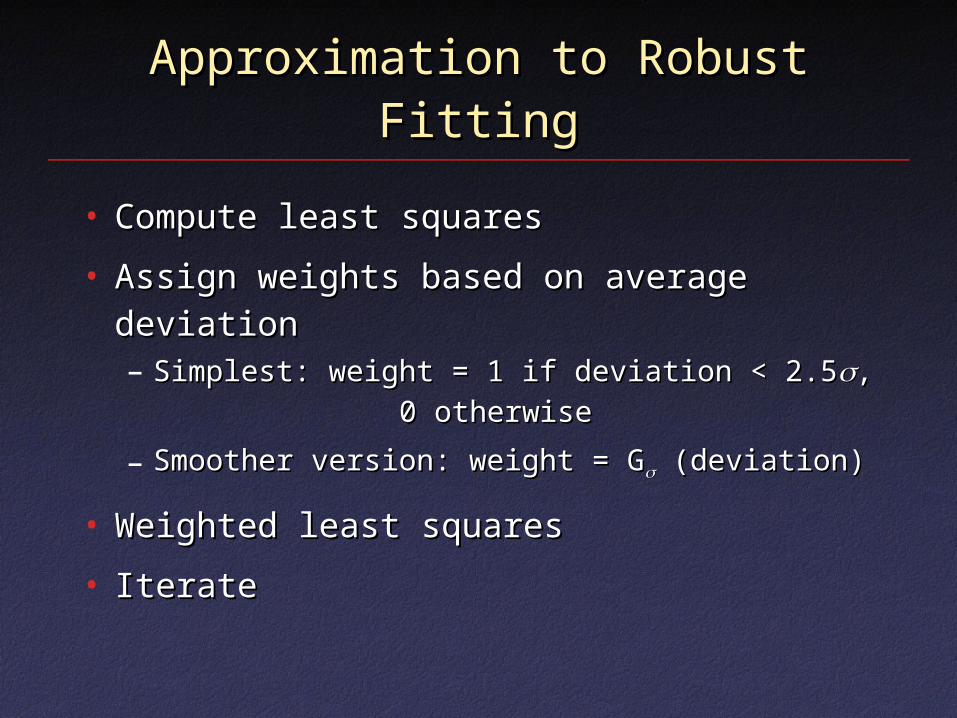
Approximation to Robust FittingApproximation to Robust Fitting
• Compute least squaresCompute least squares
• Assign weights based on average Assign weights based on average deviationdeviation– Simplest: weight = 1 if deviation < 2.5Simplest: weight = 1 if deviation < 2.5,,
0 otherwise 0 otherwise
– Smoother version: weight = GSmoother version: weight = G (deviation) (deviation)
• Weighted least squaresWeighted least squares
• IterateIterate
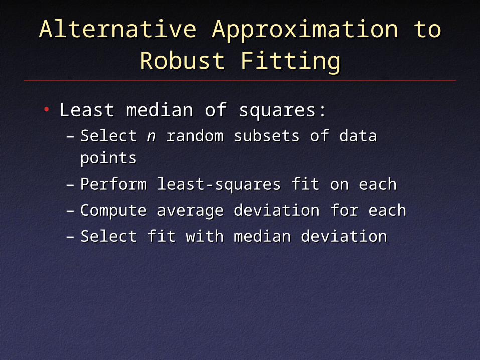
Alternative Approximation toAlternative Approximation toRobust FittingRobust Fitting
• Least median of squares:Least median of squares:– Select Select nn random subsets of data points random subsets of data points
– Perform least-squares fit on eachPerform least-squares fit on each
– Compute average deviation for eachCompute average deviation for each
– Select fit with median deviationSelect fit with median deviation

Correspondence ApproachesCorrespondence Approaches
• Optical flowOptical flow
• CorrelationCorrelation
• Correlation + optical flowCorrelation + optical flow
• Any of the above, iterated (e.g. Lucas-Any of the above, iterated (e.g. Lucas-Kanade)Kanade)
• Any of the above, coarse-to-fineAny of the above, coarse-to-fine

Correlation / Search MethodsCorrelation / Search Methods
• Assume translation onlyAssume translation only
• Given images IGiven images I11, I, I22
• For each translation (For each translation (ttxx, , ttyy) compute) compute
• Select translation that maximizes Select translation that maximizes cc
• Depending on window size, local or globalDepending on window size, local or global
i j
yx tjtiIjiIIIc ),(),,(),,( 2121 t i j
yx tjtiIjiIIIc ),(),,(),,( 2121 t

Cross-CorrelationCross-Correlation
• Statistical definition of correlation:Statistical definition of correlation:
• Disadvantage: sensitive to local Disadvantage: sensitive to local variations in image brightnessvariations in image brightness
uvvu ),( uvvu ),(

Normalized Cross-CorrelationNormalized Cross-Correlation
• Normalize to eliminate brightness Normalize to eliminate brightness sensitivity:sensitivity:
wherewhere
vu
vvuuvu
))((
),(
vu
vvuuvu
))((
),(
)deviation( standard
)average(
u
uu
u
)deviation( standard
)average(
u
uu
u

Sum of Squared DifferencesSum of Squared Differences
• More intuitive measure:More intuitive measure:
• Negative sign so that higher values Negative sign so that higher values mean greater similaritymean greater similarity
• Expand:Expand:
2)(),( vuvu 2)(),( vuvu
uvvuvu 2)( 222 uvvuvu 2)( 222

Local vs. GlobalLocal vs. Global
• Correlation with local windows not too Correlation with local windows not too expensiveexpensive
• High cost if window size = whole imageHigh cost if window size = whole image
• But computation looks like convolutionBut computation looks like convolution– FFT to the rescue!FFT to the rescue!

CorrelationCorrelation
)()()(
),(),,(
2translated1
21
IIc
jiIjiIci j
yx
FFF
)()()(
),(),,(
2translated1
21
IIc
jiIjiIci j
yx
FFF

Fourier Transform with Fourier Transform with TranslationTranslation
)(),(),( yxi yxeyxfyyxxf FF )(),(),( yxi yxeyxfyyxxf FF

Fourier Transform with Fourier Transform with TranslationTranslation
• Therefore, if ITherefore, if I11 and I and I22 differ by differ by
translation,translation,
• So, So, FF-1-1(F(F11/F/F22) will have a peak at () will have a peak at (x,x,y)y)
2
1)(
)(21 ),(),(
F
Fe
eyxIyxI
yxi
yxi
yx
yx
FF
2
1)(
)(21 ),(),(
F
Fe
eyxIyxI
yxi
yxi
yx
yx
FF
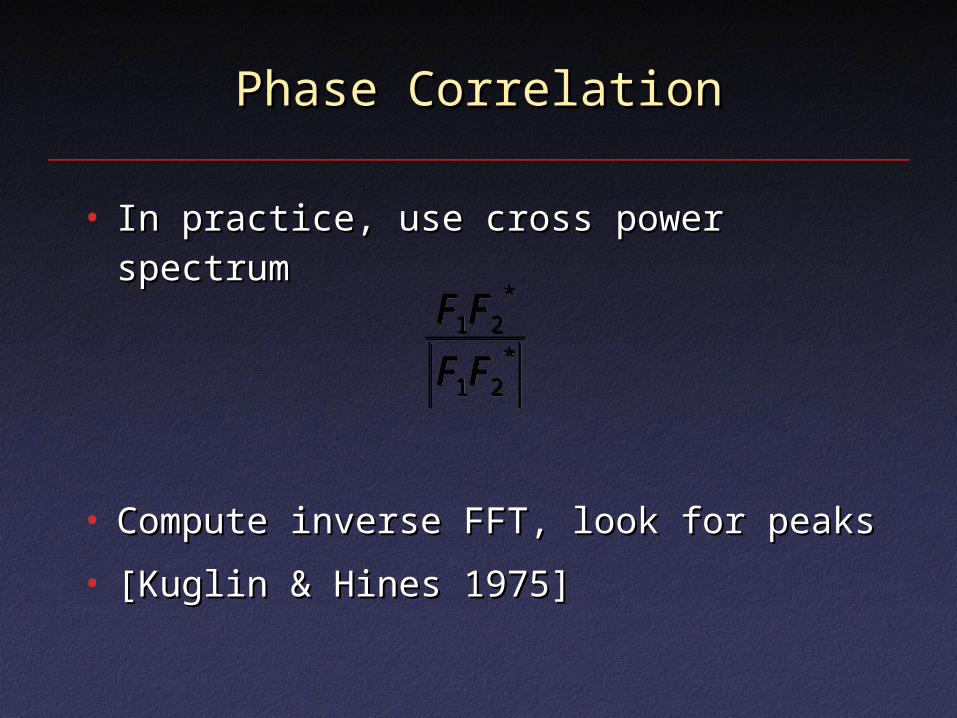
Phase CorrelationPhase Correlation
• In practice, use cross power spectrumIn practice, use cross power spectrum
• Compute inverse FFT, look for peaksCompute inverse FFT, look for peaks
• [Kuglin & Hines 1975][Kuglin & Hines 1975]
*21
*21
FF
FF*
21
*21
FF
FF

Phase CorrelationPhase Correlation
• AdvantagesAdvantages– Fast computationFast computation
– Low sensitivity to global brightness changesLow sensitivity to global brightness changes(since equally sensitive to all frequencies)(since equally sensitive to all frequencies)
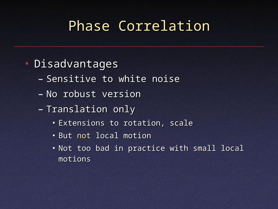
Phase CorrelationPhase Correlation
• DisadvantagesDisadvantages– Sensitive to white noiseSensitive to white noise
– No robust versionNo robust version
– Translation onlyTranslation only• Extensions to rotation, scaleExtensions to rotation, scale
• But But notnot local motion local motion
• Not too bad in practice with small local motionsNot too bad in practice with small local motions

Correspondence ApproachesCorrespondence Approaches
• Optical flowOptical flow
• CorrelationCorrelation
• Correlation + optical flowCorrelation + optical flow
• Any of the above, iterated (e.g. Lucas-Any of the above, iterated (e.g. Lucas-Kanade)Kanade)
• Any of the above, coarse-to-fineAny of the above, coarse-to-fine

Correlation plus Optical FlowCorrelation plus Optical Flow
• Use e.g. phase correlation to find Use e.g. phase correlation to find average translation (may be large)average translation (may be large)
• Use optical flow to find local motionsUse optical flow to find local motions

Correspondence ApproachesCorrespondence Approaches
• Optical flowOptical flow
• CorrelationCorrelation
• Correlation + optical flowCorrelation + optical flow
• Any of the above, iterated (e.g. Lucas-Any of the above, iterated (e.g. Lucas-Kanade)Kanade)
• Any of the above, coarse-to-fineAny of the above, coarse-to-fine

Image PyramidsImage Pyramids
• Pre-filter images to collect information Pre-filter images to collect information at different scalesat different scales
• More efficient computation, allowsMore efficient computation, allowslarger motionslarger motions

Image PyramidsImage Pyramids
SzeliskiSzeliski

Pyramid CreationPyramid Creation
• ““Gaussian” PyramidGaussian” Pyramid
• ““Laplacian” PyramidLaplacian” Pyramid– Created from GaussianCreated from Gaussian
pyramid by subtractionpyramid by subtractionLLii = G = Gii – expand(G – expand(Gi+1i+1))
SzeliskiSzeliski

Octaves in the Spatial DomainOctaves in the Spatial Domain
Bandpass ImagesBandpass Images
Lowpass Images
SzeliskiSzeliski

BlendingBlending
• Blend over too small a region: seamsBlend over too small a region: seams
• Blend over too large a region: ghostingBlend over too large a region: ghosting

Multiresolution BlendingMultiresolution Blending
• Different blending regions for different Different blending regions for different levels in a pyramid [Burt & Adelson]levels in a pyramid [Burt & Adelson]– Blend low frequencies over large regions Blend low frequencies over large regions
(minimize seams due to brightness (minimize seams due to brightness variations)variations)
– Blend high frequencies over small regions Blend high frequencies over small regions (minimize ghosting)(minimize ghosting)

Pyramid BlendingPyramid Blending
SzeliskiSzeliski

Minimum-Cost CutsMinimum-Cost Cuts
• Instead of blending high frequencies Instead of blending high frequencies along a straight line, blend along line of along a straight line, blend along line of minimum differences in image minimum differences in image intensitiesintensities

Minimum-Cost CutsMinimum-Cost Cuts
Moving object, simple blending Moving object, simple blending blur blur
[Davis 98][Davis 98]

Minimum-Cost CutsMinimum-Cost Cuts
Minimum-cost cut Minimum-cost cut no blur no blur
[Davis 98][Davis 98]
Feature TrackingFeature Tracking
• Local regionLocal region
• Take advantage of many framesTake advantage of many frames– Prediction, uncertainty estimationPrediction, uncertainty estimation
– Noise filteringNoise filtering
– Handle short occlusionsHandle short occlusions

Kalman FilteringKalman Filtering
• Assume that results of experimentAssume that results of experiment(i.e., optical flow) are noisy(i.e., optical flow) are noisymeasurements of system statemeasurements of system state
• Model of how system evolvesModel of how system evolves
• Prediction / correction frameworkPrediction / correction framework
• Optimal combinationOptimal combinationof system model and observationsof system model and observations
Rudolf Emil KalmanRudolf Emil Kalman
Acknowledgment: much of the following material is Acknowledgment: much of the following material is based on thebased on theSIGGRAPH 2001 course by Greg Welch and Gary SIGGRAPH 2001 course by Greg Welch and Gary Bishop (UNC)Bishop (UNC)

Simple ExampleSimple Example
• Measurement of a single point zMeasurement of a single point z11
• Variance Variance 1122 (uncertainty (uncertainty 11))
• Best estimate of true position Best estimate of true position
• Uncertainty in best estimateUncertainty in best estimate
11̂ zx 11̂ zx 22
1 1ˆ 22
1 1ˆ
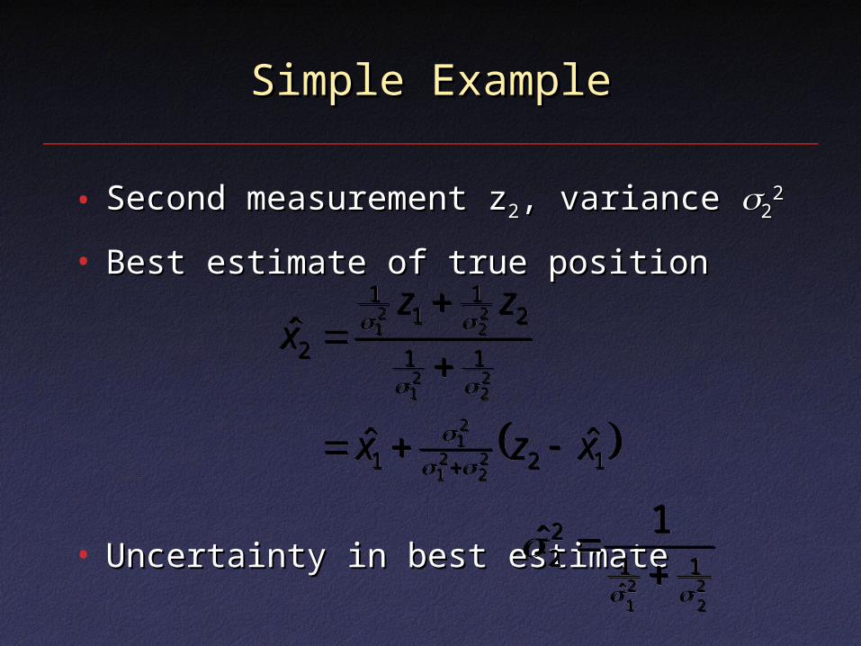
Simple ExampleSimple Example
• Second measurement zSecond measurement z22, variance , variance 2222
• Best estimate of true position Best estimate of true position
• Uncertainty in best estimateUncertainty in best estimate
121
11
21
11
2
ˆˆ
ˆ
22
21
21
22
21
22
21
xzx
zzx
121
11
21
11
2
ˆˆ
ˆ
22
21
21
22
21
22
21
xzx
zzx
22
21
1ˆ1
22
1ˆ
22
21
1ˆ1
22
1ˆ
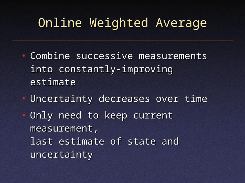
Online Weighted AverageOnline Weighted Average
• Combine successive measurements into Combine successive measurements into constantly-improving estimateconstantly-improving estimate
• Uncertainty decreases over timeUncertainty decreases over time
• Only need to keep current Only need to keep current measurement,measurement,last estimate of state and uncertaintylast estimate of state and uncertainty

TerminologyTerminology
• In this example, position is In this example, position is statestate(in general, any vector)(in general, any vector)
• State can be assumed to evolve over time State can be assumed to evolve over time according to a according to a system modelsystem model or or process process modelmodel(in this example, “nothing changes”)(in this example, “nothing changes”)
• Measurements (possibly incomplete, possibly Measurements (possibly incomplete, possibly noisy) according to a noisy) according to a measurement modelmeasurement model
• Best estimate of state with covariance Best estimate of state with covariance PPx̂x̂

Linear ModelsLinear Models
• For “standard” Kalman filtering, For “standard” Kalman filtering, everythingeverythingmust be linearmust be linear
• System model:System model:
• The matrix The matrix kk is is state transition matrixstate transition matrix
• The vector The vector kk represents represents additive noiseadditive noise,,
assumed to have covariance assumed to have covariance QQ
111 kkkk xx 111 kkkk xx
Linear ModelsLinear Models
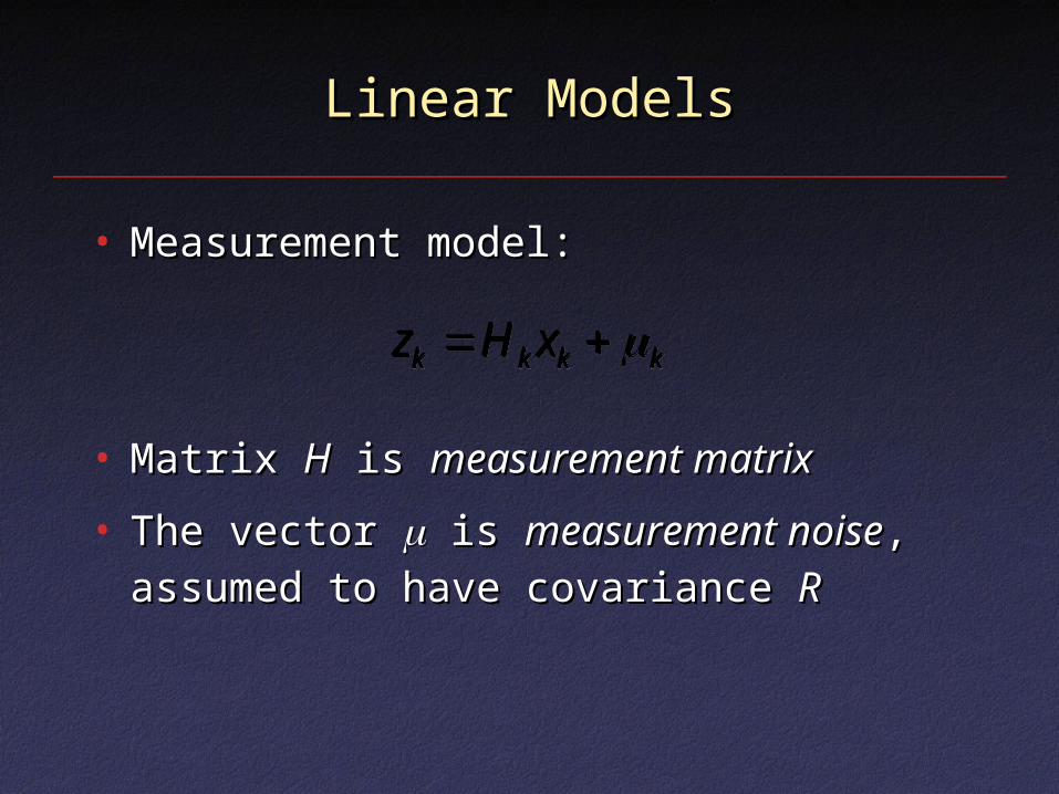
• Measurement model:Measurement model:
• Matrix Matrix HH is is measurement matrixmeasurement matrix
• The vector The vector is is measurement noisemeasurement noise,,assumed to have covariance assumed to have covariance RR
kkkk xHz kkkk xHz
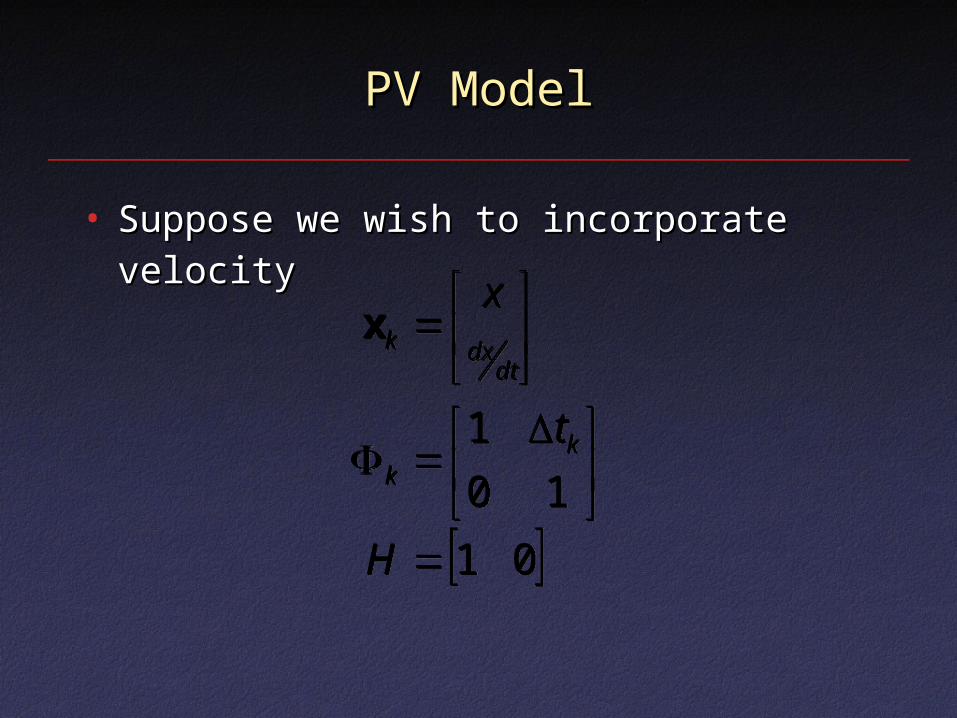
PV ModelPV Model
• Suppose we wish to incorporate velocitySuppose we wish to incorporate velocity
01
10
1
H
t
x
kk
dtdxkx
01
10
1
H
t
x
kk
dtdxkx

Prediction/CorrectionPrediction/Correction
• Predict new statePredict new state
• Correct to take new measurements into Correct to take new measurements into accountaccount
1T
111
11 ˆ
kkkkk
kkk
QPP
xx
1T
111
11 ˆ
kkkkk
kkk
QPP
xx
kkkk
kkkkkk
PHKIP
xHzKxx
ˆ kkkk
kkkkkk
PHKIP
xHzKxx
ˆ

Kalman GainKalman Gain
• Weighting of process model vs. Weighting of process model vs. measurementsmeasurements
• Compare to what we saw earlier:Compare to what we saw earlier:
1TT kkkkkkk RHPHHPK 1TT kkkkkkk RHPHHPK
22
21
21
2
221
21

Results: Position-Only ModelResults: Position-Only Model
MovingMoving StillStill
[Welch & Bishop][Welch & Bishop]

Results: Position-Velocity ModelResults: Position-Velocity Model
[Welch & Bishop][Welch & Bishop]
MovingMoving StillStill

Extension: Multiple ModelsExtension: Multiple Models
• Simultaneously run many KFs with Simultaneously run many KFs with different system modelsdifferent system models
• Estimate probability each KF is correctEstimate probability each KF is correct
• Final estimate: weighted averageFinal estimate: weighted average

Results: Multiple ModelsResults: Multiple Models
[Welch & Bishop][Welch & Bishop]
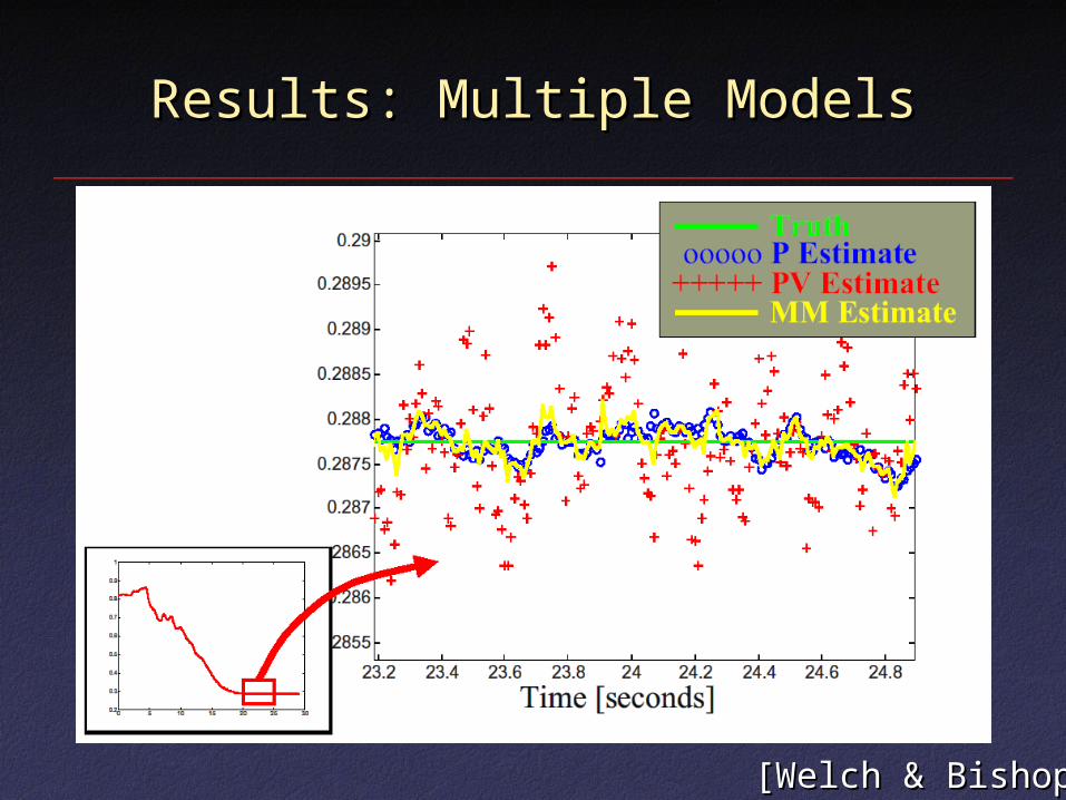
Results: Multiple ModelsResults: Multiple Models
[Welch & Bishop][Welch & Bishop]

Results: Multiple ModelsResults: Multiple Models
[Welch & Bishop][Welch & Bishop]

Extension: SCAATExtension: SCAAT
• HH be different at different times be different at different times– Different sensors, types of measurementsDifferent sensors, types of measurements
– Sometimes measure only part of stateSometimes measure only part of state
• Single Constraint At A Time (SCAAT)Single Constraint At A Time (SCAAT)– Incorporate results from one sensor at onceIncorporate results from one sensor at once
– Alternative: wait until you have measurements Alternative: wait until you have measurements from enough sensors to know complete state from enough sensors to know complete state (MCAAT)(MCAAT)
– MCAAT equations often more complex, but MCAAT equations often more complex, but sometimes necessary for initializationsometimes necessary for initialization
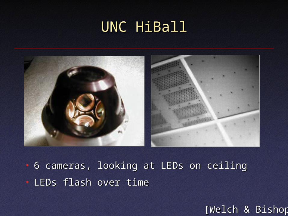
UNC HiBallUNC HiBall
• 6 cameras, looking at LEDs on ceiling6 cameras, looking at LEDs on ceiling
• LEDs flash over timeLEDs flash over time
[Welch & Bishop][Welch & Bishop]

Extension: Nonlinearity (EKF)Extension: Nonlinearity (EKF)
• HiBall state model has nonlinear degrees of HiBall state model has nonlinear degrees of freedom (rotations)freedom (rotations)
• Extended Kalman Filter allows Extended Kalman Filter allows nonlinearities by:nonlinearities by:– Using general functions instead of matricesUsing general functions instead of matrices
– Linearizing functions to project forwardLinearizing functions to project forward
– Like 1Like 1stst order Taylor series expansion order Taylor series expansion
– Only have to evaluate Jacobians (partial Only have to evaluate Jacobians (partial derivatives), not invert process/measurement derivatives), not invert process/measurement functionsfunctions

Other ExtensionsOther Extensions
• On-line noise estimationOn-line noise estimation
• Using known system input (e.g. Using known system input (e.g. actuators)actuators)
• Using information from both past and Using information from both past and futurefuture
• Non-Gaussian noise and particle Non-Gaussian noise and particle filteringfiltering