image compression using singular value decomposition...

Image Compression using Singular Value

Decomposition (SVD)

by Brady Mathews

12 December 2014

The University of Utah

(1) What is the Singular Value Decomposition?

Linear Algebra is a study that works mostly with math on matrices. A matrix is just a

table that holds data, storing numbers in columns and rows. Linear Algebra then takes these

matrices and tries to manipulate them which allows for us to analyze large portions of data. This

paper will be discussing one of these large portions of data as we talk about image compression

later on where each pixel can be represented as a number, and the columns and rows of the

matrix hold the position of that value relative to where it is on the image.

First however, let us talk about what the Singular Value Decomposition, or SVD for short, is.

When given a matrix, there are several important values that mathematicians can derive from

them that help explain what the data represents, classify the data into families, and they can also

manipulate matrices by pulling them apart into values that are easier to work with, then stitching

those values back together at the end of the computation to obtain some type of result. The SVD

is one such computation which mathematicians find extremely useful.

What the SVD does is split a matrix into three important sub matrices to represent the data.

Given the matrix A, where the size of a is 𝑚 × 𝑛 where 𝑚 represents the number of rows in the

matrix, and 𝑛 represents the number of columns, A can be broken down into three sub matrices

𝐴 = 𝑈Σ𝑉𝑇 where 𝑈 is of size 𝑚 × 𝑚, Σ is of size 𝑚 × 𝑛 and is diagonal, and 𝑉𝑇is of size 𝑛 × 𝑛.

It is required for matrix multiplication that the size of the columns of the first matrix must match

up with the size of the rows of the second matrix. When you multiply a matrix of size 𝑎 × 𝑏 and

a matrix of size 𝑏 × 𝑐, the resulting matrix will yield a matrix of size 𝑎 × 𝑐.

So, abstracting the matrices into their size components, we can see that this multiplication will

yield a matrix of the same size:

𝑚 × 𝑛 = [(𝑚 × 𝑚)(𝑚 × 𝑛)](𝑛 × 𝑛)

𝑚 × 𝑛 = (𝑚 × 𝑛)(𝑛 × 𝑛)

𝑚 × 𝑛 = (𝑚 × 𝑛)

Now, the interesting part of these matrices “𝑈Σ𝑉𝑇” are that the data is arrange in such a way that

the most important data is stored on the top. 𝑈 is a matrix that holds important information

about the rows of the matrix, and the most important information about the matrix is stored on

the first column. 𝑉𝑇 is a matrix that holds important information about the columns of each

matrix, and the most important information about the matrix is stored on the first row. Σ is a

diagonal matrix which will only have at most “𝑚” important values, the rest of the matrix being

zero. Because the important numbers of this matrix are only stored on the diagonal, we will

ignore this for size comparison.

Key point: The reason why the SVD is computed is because you can use the first components of

these matrices to give you a close approximation of what the actual matrix looked like. Going

back to our size example, if the most important information of 𝑈 is stored on its first column,

then 𝑈’s important information can be written as an (𝑚 × 1) matrix. If the most important

information of 𝑉𝑇 is stored on its first row, then 𝑉𝑇’s important information can be written as a

(1 × 𝑛) matrix. We will also say that the important information of Σ is stored on the first row,

first column of that matrix, yielding a (1 × 1) matrix. By multiplying these matrices together:

𝑈′Σ′𝑉𝑇′= [( 𝑚 × 1)(1 × 1)](1 × 𝑛)

= ( 𝑚 × 1)(1 × 𝑛)

= ( 𝑚 × 𝑛)

We can see that the resulting computation is the same size as the original matrix. This resulting

matrix, which we will call 𝐴′, is a good approximation of the original matrix 𝐴. For an even

closer approximation, you include the next column of 𝑈 and the next row of 𝑉𝑇. But where do

these magic matrices come from? Linear algebra holds the mystery.

(2) Computing the SVD

Now we will get into the math and theory behind what I just described above. We will go

through an example to solve the equation 𝐴 = 𝑈Σ𝑉𝑇.

Given 𝐴 = [2

−1 2 1

00 ] find the SVD:

The first thing we need to find in this computation is finding the matrix 𝐴𝑇𝐴. The superscript T

stands for “transpose” which to put nicely, you flip the matrix on its side, row one becoming

column one.

[2 −12 10 0

] [2 2 0

−1 1 0 ] = [

5 3 03 5 00 0 0

]

If you’re not a mathematician, matrix multiplication works likes so. To get the first row, first

column of the resulting matrix, you need to take the first row of the first matrix, and the first

column of the second matrix. Then you multiply the corresponding first values together, and the

corresponding second values together etc., and then sum those values.

Therefore, first row first column: [2 −1 ] [2

−1] will yield (2 × 2) + (−1 × −1) = 4 + 1 = 5

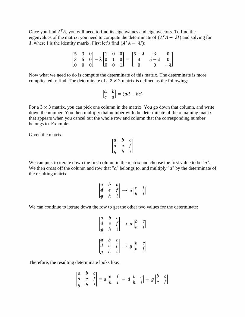
Once you find 𝐴𝑇𝐴, you will need to find its eigenvalues and eigenvectors. To find the

eigenvalues of the matrix, you need to compute the determinate of (𝐴𝑇𝐴 − 𝜆𝐼) and solving for

𝜆, where I is the identity matrix. First let’s find (𝐴𝑇𝐴 − 𝜆𝐼):

[5 3 03 5 00 0 0

] − 𝜆 [1 0 00 1 00 0 1

] = [5 − 𝜆 3 0

3 5 − 𝜆 00 0 −𝜆

]

Now what we need to do is compute the determinate of this matrix. The determinate is more

complicated to find. The determinate of a 2 × 2 matrix is defined as the following:

|𝑎 𝑏𝑐 𝑑

| = (𝑎𝑑 − 𝑏𝑐)

For a 3 × 3 matrix, you can pick one column in the matrix. You go down that column, and write

down the number. You then multiply that number with the determinate of the remaining matrix

that appears when you cancel out the whole row and column that the corresponding number

belongs to. Example:

Given the matrix:

[𝑎 𝑏 𝑐𝑑 𝑒 𝑓𝑔 ℎ 𝑖

]

We can pick to iterate down the first column in the matrix and choose the first value to be "𝑎". We then cross off the column and row that "𝑎" belongs to, and multiply "𝑎" by the determinate of

the resulting matrix.

|𝑎 𝑏 𝑐𝑑 𝑒 𝑓𝑔 ℎ 𝑖

| ⟶ 𝑎 |𝑒 𝑓ℎ 𝑖

|

We can continue to iterate down the row to get the other two values for the determinate:


| ⟶ 𝑑 |𝑏 𝑐ℎ 𝑖

|


| ⟶ 𝑔 |𝑏 𝑐𝑒 𝑓

|

Therefore, the resulting determinate looks like:


| = 𝑎 |𝑒 𝑓ℎ 𝑖

| − 𝑑 |𝑏 𝑐ℎ 𝑖

| + 𝑔 |𝑏 𝑐𝑒 𝑓

|

You do sum the result, but we have the subtraction in the second term because there is really an

invisible (−1)𝑥+𝑦 multiplied to each term, where “x” is the row number and “y” is the column

number. Going back to our definition of how to solve the determinate of a 2 × 2 matrix, we get:

𝑎(𝑒𝑖 − 𝑓ℎ) + 𝑑(𝑏𝑖 − ℎ𝑐) + 𝑔(𝑏𝑓 − 𝑐𝑒)

Now in our example matrix, we have a lot of zeros in column 3, so instead let’s iterate down

colum3 to compute our result.

|5 − 𝜆 3 0

3 5 − 𝜆 00 0 −𝜆

| = 0 |3 5 − 𝜆0 0

| − 0 |5 − 𝜆 3

0 0| + (−𝜆) |

5 − 𝜆 33 5 − 𝜆

|

Since zero multiplied by anything is zero, we can drop the first two terms:

|5 − 𝜆 3 0

3 5 − 𝜆 00 0 −𝜆

| = −𝜆 |5 − 𝜆 3

3 5 − 𝜆|

Computing the 2 × 2 matrix we get:

|5 − 𝜆 3 0

3 5 − 𝜆 00 0 −𝜆

| = −𝜆((5 − 𝜆)(5 − 𝜆) − (3)(3))

|5 − 𝜆 3 0

3 5 − 𝜆 00 0 −𝜆

| = −𝜆(𝜆2 − 10𝜆 + 16)

Now we can solve to find when 𝜆 = 0 to find our eigenvalues:

−𝜆(𝜆2 − 10𝜆 + 16) = −𝜆(𝜆 − 2)(𝜆 − 8)

Therefore or eigenvalues are 8, 2, and 0. You will want to keep these numbers in descending

order.

With this information, we can find an important value "𝜎" which is the square root of the

eigenvalues. We ignore zero for the "𝜎" term. Therefore:

𝜎1 = √8 = 2√2 and 𝜎2 = 2

These values are the important values along the diagonal of matrix "Σ".

Next we need to find the normalized version of the corresponding eigenvectors to each of the

eigenvalues. To find an eigenvalue, replace 𝜆 with the corresponding eigenvalue in the equation

(𝐴𝑇𝐴 − 𝜆𝐼). Then find the nullspace of that resulting matrix:

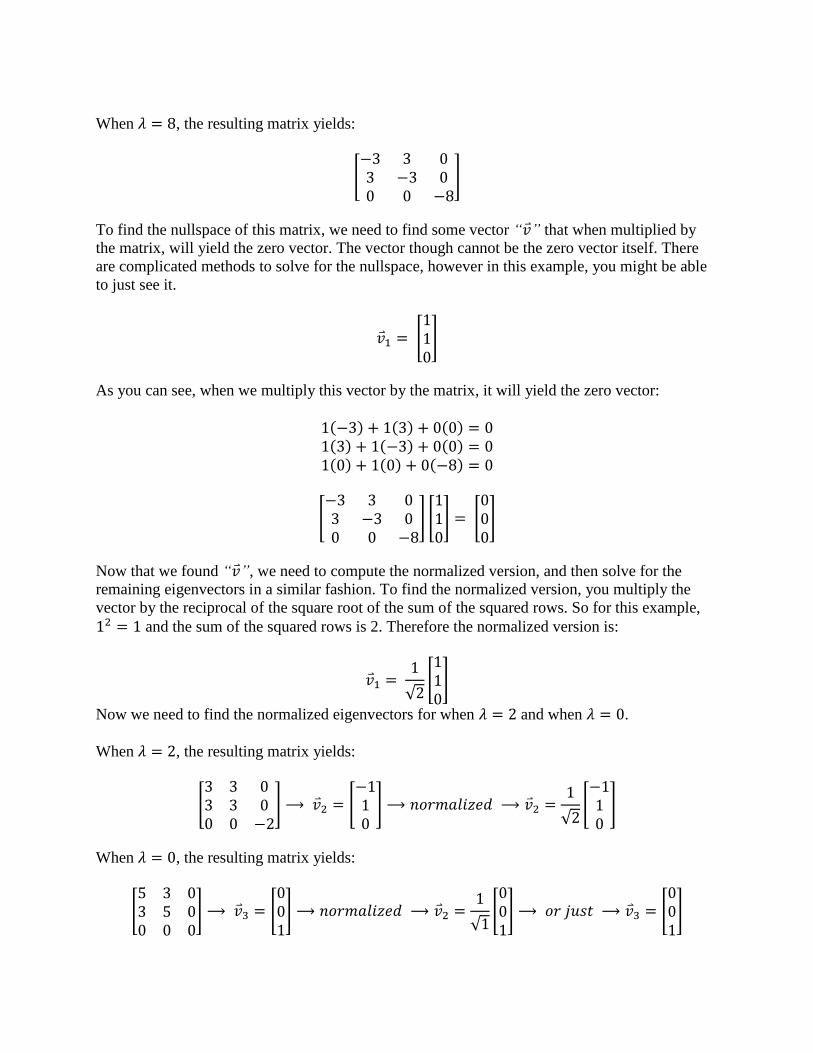
When 𝜆 = 8, the resulting matrix yields:

[−3 3 03 −3 00 0 −8

]

To find the nullspace of this matrix, we need to find some vector “�⃑�” that when multiplied by

the matrix, will yield the zero vector. The vector though cannot be the zero vector itself. There

are complicated methods to solve for the nullspace, however in this example, you might be able

to just see it.

�⃑�1 = [110]

As you can see, when we multiply this vector by the matrix, it will yield the zero vector:

1(−3) + 1(3) + 0(0) = 0

1(3) + 1(−3) + 0(0) = 0

1(0) + 1(0) + 0(−8) = 0

[−3 3 03 −3 00 0 −8

] [110] = [

000]

Now that we found “�⃑�”, we need to compute the normalized version, and then solve for the

remaining eigenvectors in a similar fashion. To find the normalized version, you multiply the

vector by the reciprocal of the square root of the sum of the squared rows. So for this example,

12 = 1 and the sum of the squared rows is 2. Therefore the normalized version is:

�⃑�1 = 1

√2[110]

Now we need to find the normalized eigenvectors for when 𝜆 = 2 and when 𝜆 = 0.


[3 3 03 3 00 0 −2

] ⟶ �⃑�2 = [−110

] ⟶ 𝑛𝑜𝑟𝑚𝑎𝑙𝑖𝑧𝑒𝑑 ⟶ �⃑�2 =1

√2[−110

]


[5 3 03 5 00 0 0

] ⟶ �⃑�3 = [001] ⟶ 𝑛𝑜𝑟𝑚𝑎𝑙𝑖𝑧𝑒𝑑 ⟶ �⃑�2 =

1

√1[001] ⟶ 𝑜𝑟 𝑗𝑢𝑠𝑡 ⟶ �⃑�3 = [

001]

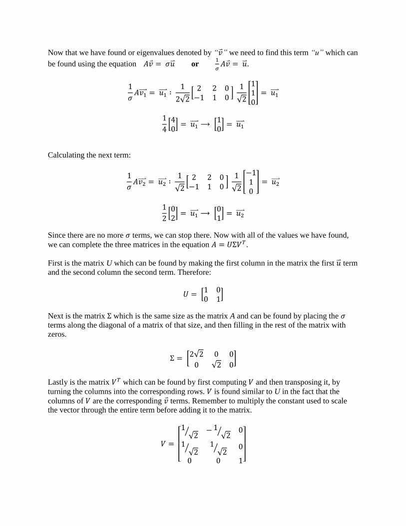
Now that we have found or eigenvalues denoted by “�⃑�” we need to find this term “u” which can

be found using the equation 𝐴�⃑� = 𝜎�⃑⃑� or 1

𝜎𝐴�⃑� = �⃑⃑�.

1

𝜎𝐴𝑣1⃑⃑⃑⃑⃑ = 𝑢1⃑⃑⃑⃑⃑ ∶

1

2√2[

2 2 0−1 1 0

] 1

√2[110] = 𝑢1⃑⃑⃑⃑⃑

1

4[40] = 𝑢1⃑⃑⃑⃑⃑ ⟶ [

10] = 𝑢1⃑⃑⃑⃑⃑

Calculating the next term:

1

𝜎𝐴𝑣2⃑⃑⃑⃑⃑ = 𝑢2⃑⃑⃑⃑⃑ ∶

1

√2[

2 2 0−1 1 0

] 1

√2[−110

] = 𝑢2⃑⃑⃑⃑⃑

1

2[02] = 𝑢1⃑⃑⃑⃑⃑ ⟶ [

01] = 𝑢2⃑⃑⃑⃑⃑

Since there are no more 𝜎 terms, we can stop there. Now with all of the values we have found,

we can complete the three matrices in the equation 𝐴 = 𝑈Σ𝑉𝑇.

First is the matrix U which can be found by making the first column in the matrix the first �⃑⃑� term

and the second column the second term. Therefore:

𝑈 = [1 00 1

]

Next is the matrix Σ which is the same size as the matrix A and can be found by placing the 𝜎

terms along the diagonal of a matrix of that size, and then filling in the rest of the matrix with

zeros.

Σ = [2√2 0 0

0 √2 0]

Lastly is the matrix 𝑉𝑇 which can be found by first computing 𝑉 and then transposing it, by

turning the columns into the corresponding rows. 𝑉 is found similar to U in the fact that the

columns of 𝑉 are the corresponding �⃑� terms. Remember to multiply the constant used to scale

the vector through the entire term before adding it to the matrix.

𝑉 =

[ 1

√2⁄ −1

√2⁄ 0

1√2

⁄ 1√2

⁄ 0

0 0 1]

𝑉𝑇 =

[

1√2

⁄ 1√2

⁄ 0

−1√2

⁄ 1√2

⁄ 0

0 0 1]

So now we have the finished equation 𝐴 = 𝑈Σ𝑉𝑇 yields:

[2 2 0

−1 1 0 ] = [

1 00 1

] [2√2 0 0

0 √2 0]

[

1√2

⁄ 1√2

⁄ 0

−1√2

⁄ 1√2

⁄ 0

0 0 1]

You can also multiply the terms together to show that the equation holds true. Now to move onto

the point of this paper, why do we care, and what are the real world applications.

(3) Compressing an Image

The monitor on your computer is a truly magical device. When you look at the color

white on your screen, you’re not actually looking at white, and the same thing for the color

yellow. There is actually no white or yellow pigment in your screen. What you are looking at is a

mixture of the colors red, green, and blue displayed by extremely small pixels on your screen.

These pixels are displayed in a grid like pattern, and the saturation of each pixel tricks your brain

into thinking it’s a different color entirely when looked at from a distance.

These red, green, and blue pixels range in saturation on a scale of 0 to 255; 0 being completely

off, and 255 being completely on. They can also be written in hexadecimal format like #F5C78A

for example. In hexadecimal, A is the value 10, and F is the value 15, therefore 0F = 15 and A0 =

16. The first two numbers in this string of numbers represents the red value, the next two

representing the green value, and the final two representing the blue value. To put reference into

what these are doing, here are some easy color examples:

#000000 = Black

#FFFFFF = White

#A0A0A0 = Gray

#FF0000 = Red

#00FF00 = Green

#0000FF = Blue

Because of a pixel’s grid like nature on your monitor, a picture can actually be represented as

data in a matrix. Let’s stick with a grayscale image for right now. To make an image gray, the

values for red, green, and blue need to be the same. Therefore you can represent a pixel as

having a value of 0 through 255 (in hexadecimal 00 through FF), and then repeating that value

across the red, green, and blue saturation to get the corresponding shade of gray.

Let’s say that you have a grayscale image that is 100 × 100 pixels in dimension. Each of those

pixels can be represented in a matrix that is also 100 × 100, where the values in the matrix range

from 0 to 255. Now, if you wanted to store that image, you would have to keep track of exactly

100 × 100 numbers or 10,000 different pixel values. That may not seem like a lot, but you can

also think if the image as your desktop background which is probably and image 1280 × 1024

in which you would have to store 1,310,720 different pixel values! And that’s if it was a

grayscale image, if it was colored, it would be triple that, having to keep track of 3,932,160

different numbers, which if you think about one of those numbers equating to a byte on your

computer, that equals 1.25MB for a grayscale image or 3.75MB for a colored image. Just

imagine how quickly a movie would increase in size if it was updating at the rate of 30-60

frames per second.

What we can actually do to save memory on our image is to compute the SVD and then calculate

some level of precision. You would find that in an image that is 100 × 100 pixels would look

really quite good with only 10 modes of precision using the SVD computation.

Going back to our example in section 1, “The reason why the SVD is computed is because you

can use the first components of these matrices to give you a close approximation of what the

actual matrix looked like.”

Then we calculated the first components of these matrices by taking the first column of U and

multiplying it by the first row of 𝑉𝑇. We saw that this resulted in a matrix with the dimensions of

the original matrix A.

𝑈′Σ′𝑉𝑇′= [( 𝑚 × 1)(1 × 1)](1 × 𝑛)

= ( 𝑚 × 1)(1 × 𝑛)

= ( 𝑚 × 𝑛)

Modes are how many columns of the matrix U you want to use and how many rows of the matrix

𝑉𝑇 you wanted to use to calculate your specified level of precision.

Therefore if we have a matrix 100 × 100, and we use a level of precision of 10 modes, we will

find that our matrices are:

𝑈′ = (100 × 10), Σ′ = (10 × 10), 𝑉𝑇′= (10 × 100)

So now we are only keeping track of 2,100 different numbers instead of 10,000 which greatly

increases the storage of memory. Also, if you remember how we computed Σ, it is a diagonal

matrix with values along the diagonal and zeros everywhere else. Therefore, we can represent Σ

as only being the first ten values of 𝜎, and saving only those values in memory, reconstructing

the matrix when opening the file, and Σ goes from size 100 to size 10. However, there may not

be as many 𝜎 in the computation as the size of the matrix, in a 5 × 5 matrix, you can have at

most five 𝜎’s, but you can also have as little as one, the rest of the values on the diagonal also

being zero. So really 𝜎 ≤ # modes, which is going to be so little anyway, we are going to negate

it from our computation.

That’s great in theory, but when you compute these new matrices using your specified modes of

precision, what do they actually look like? Well, using a program called “MatLab”, we can write

a program that will load in image file, turn the pixel values of the grayscale image into a matrix,

compute the SVD for us, and then convert our new matrix back into an image for our viewing

pleasure.

Figure 3.1: Image size 250x236 – modes used

{{1,2,4,6},{8,10,12,14},{16,18,20,25},{50,75,100,original image}}

In figure 3.1 we see that the image size is 250x236 pixels. By storing the image in its entirety, we

can calculate that we would need to store 59,000 different pixel values. The image starts to look

very decent along the bottom row, the last images using modes 50, 75, and 100. By negating the

size of Σ since it is so miniscule, we can calculate:

Original Image: 59,000 bytes

Mode 100: 48,600 bytes



So, these modes actually do save on memory quite a bit, more than halving the amount of

memory used at mode 50, which is represented by the bottom left image in figure 3.1.

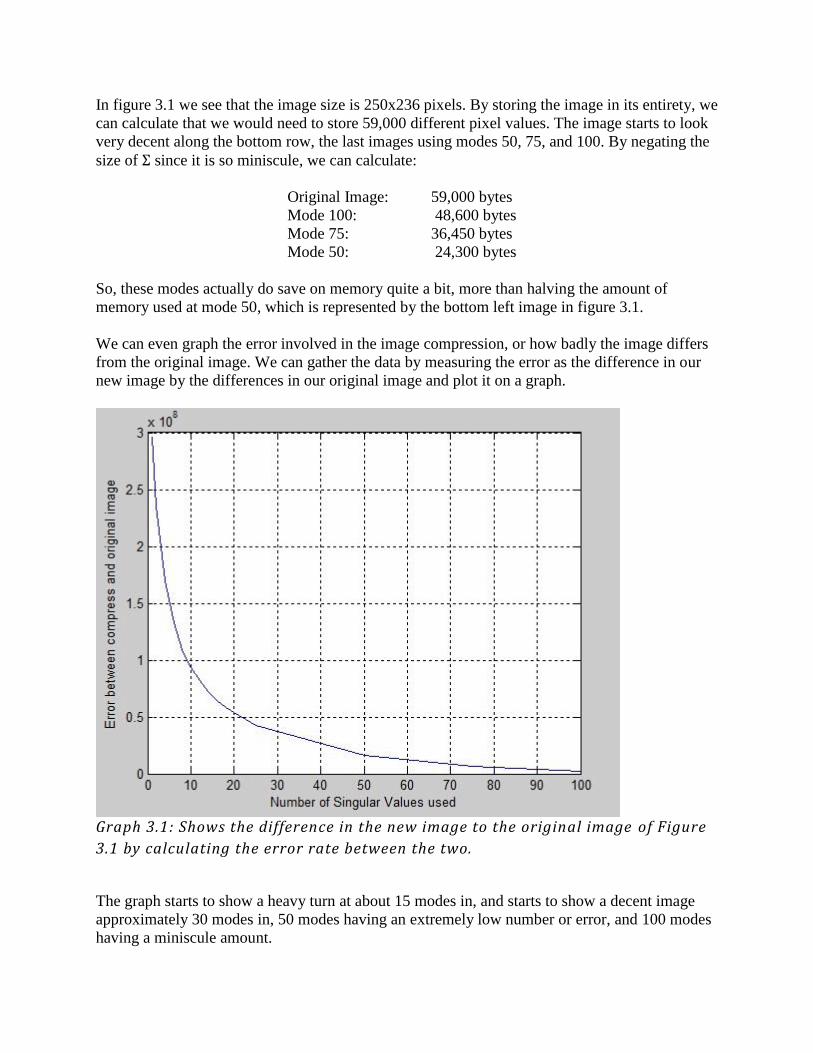
We can even graph the error involved in the image compression, or how badly the image differs

from the original image. We can gather the data by measuring the error as the difference in our

new image by the differences in our original image and plot it on a graph.

Graph 3.1: Shows the difference in the new image to the original image of Figure

3.1 by calculating the error rate between the two.

The graph starts to show a heavy turn at about 15 modes in, and starts to show a decent image

approximately 30 modes in, 50 modes having an extremely low number or error, and 100 modes

having a miniscule amount.

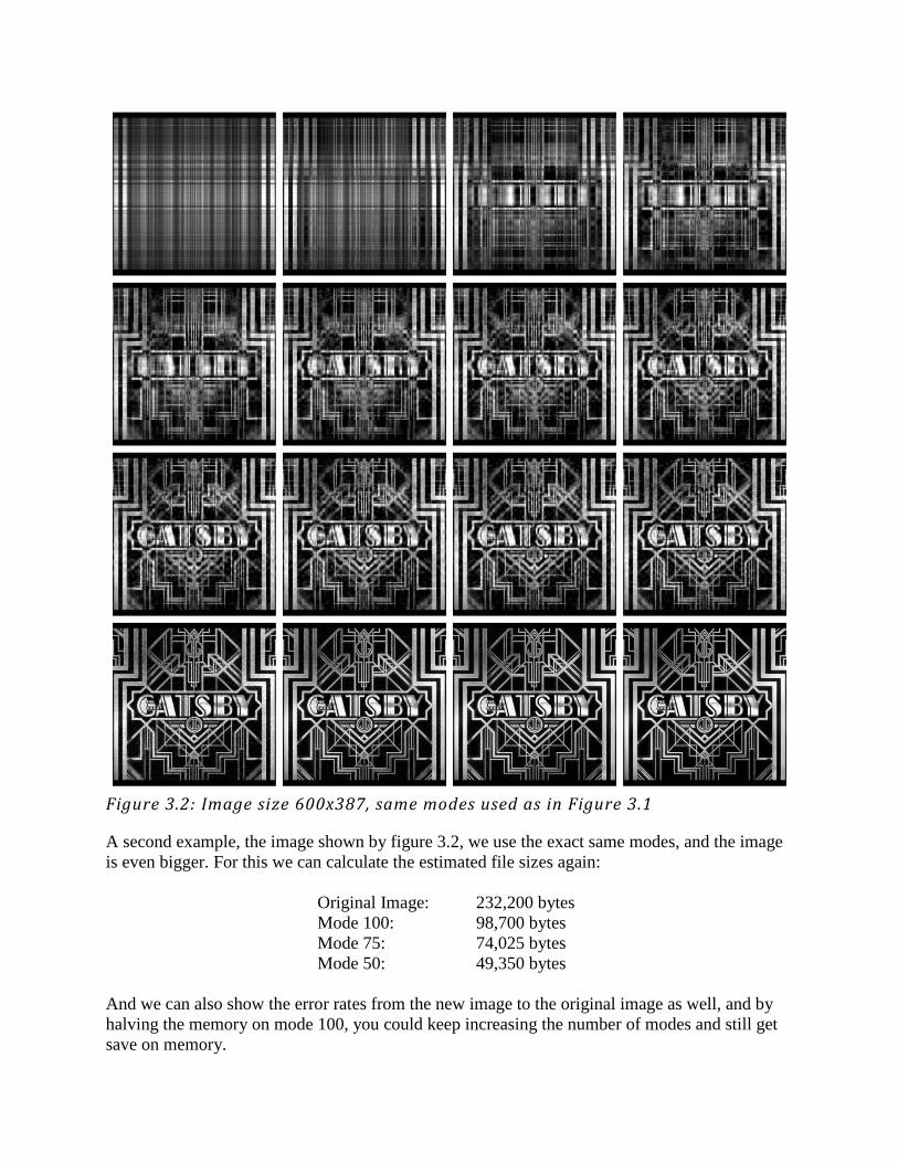
Figure 3.2: Image size 600x387, same modes used as in Figure 3.1

A second example, the image shown by figure 3.2, we use the exact same modes, and the image

is even bigger. For this we can calculate the estimated file sizes again:

Original Image: 232,200 bytes




And we can also show the error rates from the new image to the original image as well, and by

halving the memory on mode 100, you could keep increasing the number of modes and still get

save on memory.

Graph 3.2: Shows the difference in the new image to the original image of Figure

3.2 by calculating the error rate between the two.

Now we can see that this works for a grayscale image, but what about a colored image? Would

this still have the same application for image compression? The answer is a surprising yes, but it

does require a few more calculations.

The difference between a grayscale image and a colored image is that you are now storing 3

bytes of information per pixel rather than 1 byte per pixel. This is because the red, green, and

blue pixel values are now different rather than the same, so we have to represent each

individually.

First, we need to take a colored image, and split it into three new images, a red-scale, green-

scale, and blue-scale image.

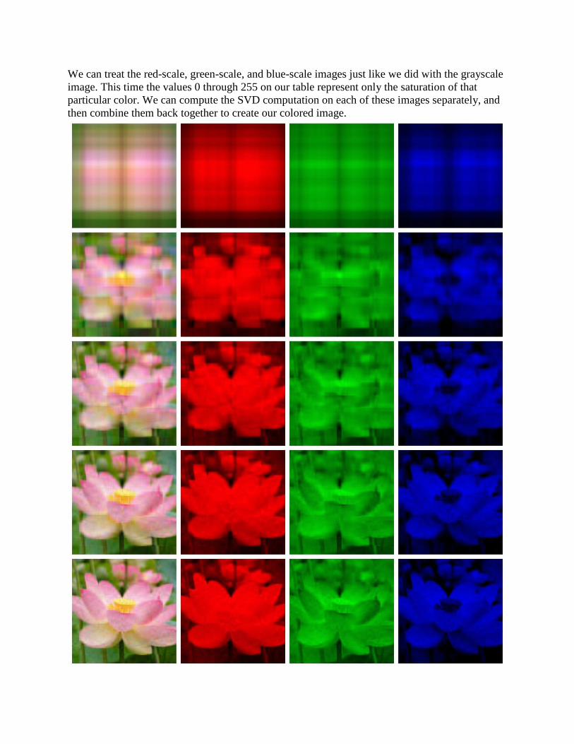
We can treat the red-scale, green-scale, and blue-scale images just like we did with the grayscale

image. This time the values 0 through 255 on our table represent only the saturation of that

particular color. We can compute the SVD computation on each of these images separately, and

then combine them back together to create our colored image.

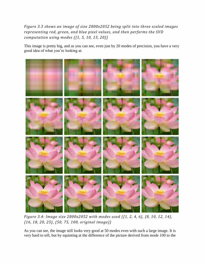
Figure 3.3 shows an image of size 2800x2052 being split into three scaled images

representing red, green, and blue pixel values, and then performs the SVD

computation using modes {{1, 5, 10, 15, 20}}

This image is pretty big, and as you can see, even just by 20 modes of precision, you have a very

good idea of what you’re looking at.

Figure 3.4: Image size 2800x2052 with modes used {{1, 2, 4, 6}, {8, 10, 12, 14},

{16, 18, 20, 25}, {50, 75, 100, original image}}

As you can see, the image still looks very good at 50 modes even with such a large image. It is

very hard to tell, but by squinting at the difference of the picture derived from mode 100 to the

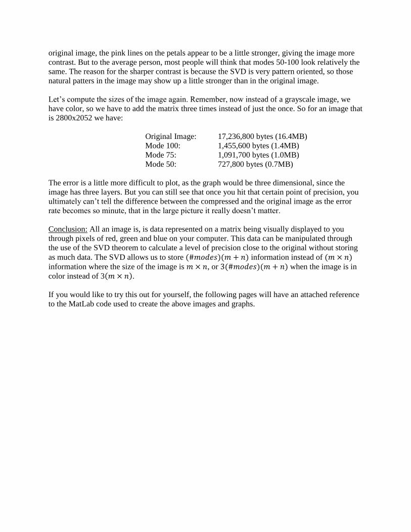
original image, the pink lines on the petals appear to be a little stronger, giving the image more

contrast. But to the average person, most people will think that modes 50-100 look relatively the

same. The reason for the sharper contrast is because the SVD is very pattern oriented, so those

natural patters in the image may show up a little stronger than in the original image.

Let’s compute the sizes of the image again. Remember, now instead of a grayscale image, we

have color, so we have to add the matrix three times instead of just the once. So for an image that

is 2800x2052 we have:

Original Image: 17,236,800 bytes (16.4MB)

Mode 100: 1,455,600 bytes (1.4MB)

Mode 75: 1,091,700 bytes (1.0MB)

Mode 50: 727,800 bytes (0.7MB)

The error is a little more difficult to plot, as the graph would be three dimensional, since the

image has three layers. But you can still see that once you hit that certain point of precision, you

ultimately can’t tell the difference between the compressed and the original image as the error

rate becomes so minute, that in the large picture it really doesn’t matter.

Conclusion: All an image is, is data represented on a matrix being visually displayed to you

through pixels of red, green and blue on your computer. This data can be manipulated through

the use of the SVD theorem to calculate a level of precision close to the original without storing

as much data. The SVD allows us to store (#𝑚𝑜𝑑𝑒𝑠)(𝑚 + 𝑛) information instead of (𝑚 × 𝑛)

information where the size of the image is 𝑚 × 𝑛, or 3(#𝑚𝑜𝑑𝑒𝑠)(𝑚 + 𝑛) when the image is in

color instead of 3(𝑚 × 𝑛).

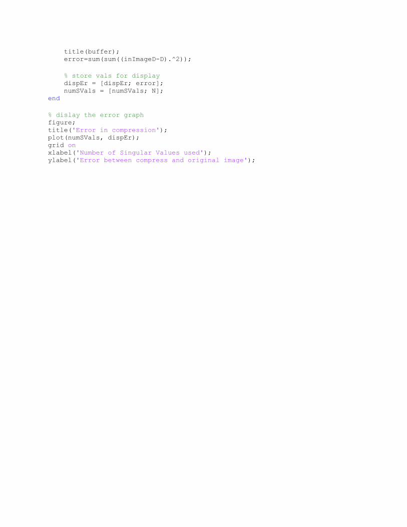
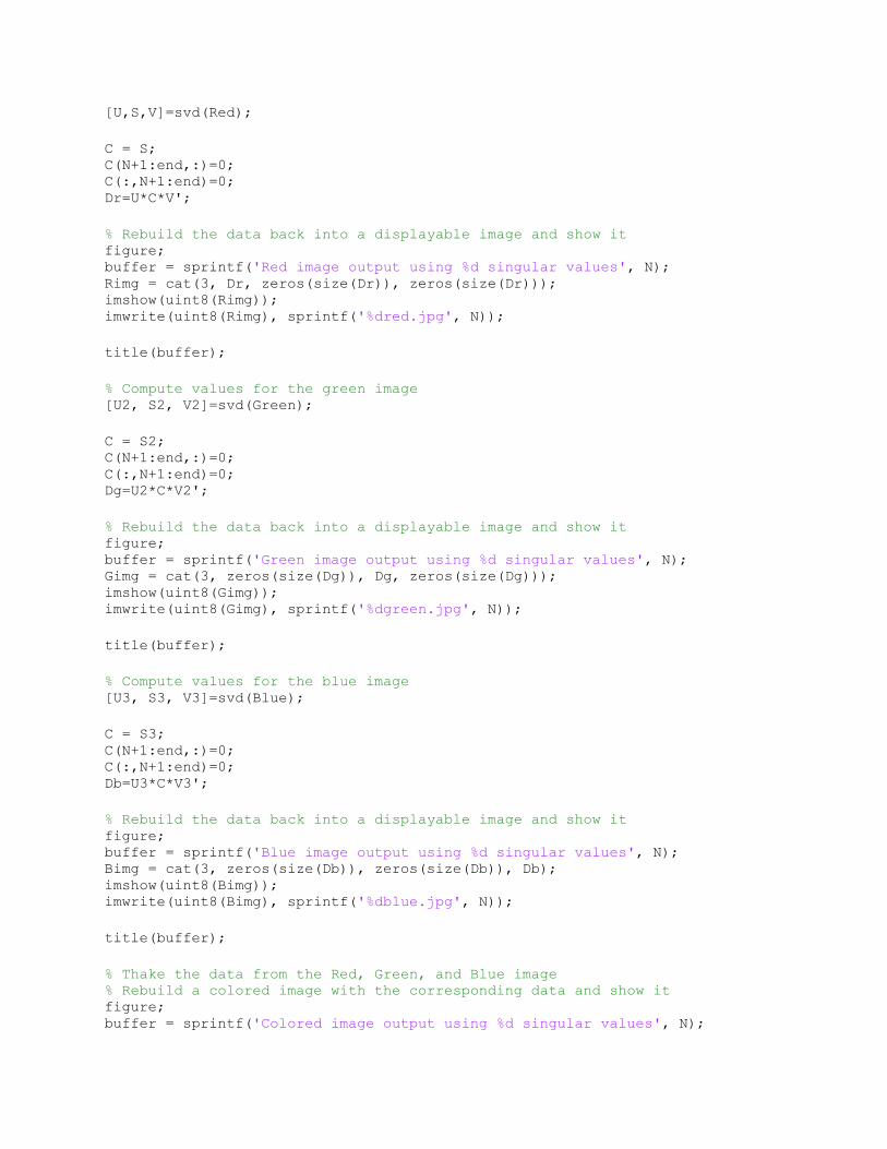
If you would like to try this out for yourself, the following pages will have an attached reference

to the MatLab code used to create the above images and graphs.

MatLab Code for GrayScale Images

% Brady Mathews - The University of Utah December 2014

% This document contains instructions for Matlab which will Open an image % file, turn the image into a grayscale format Grab the image data and % build a matrix representing each pixel value as 0-255 as data on the % matrix. It will then compute the SVD on the matrix, and display varying % different modes and levels of pressision based on the image compression, % as well as an error graph at the end on how accurate the image got based % on the difference from the original image. It will also save these % resulting images on your computer. To upload an image, replace the % "image.jpg" with the filepath, name, and data type of the image you wish % to use. If you would not like the program to save the image to your % computer, comment out or eleminate the lines that say % "imwrite(unit8(...), '%d...')"

% The following will give you modes 1, then (2,4,6,8,10,12,14,16,18,20) % then it will give you modes (25,50.75.100). To edit these, change the % value of N in the loops.

close all clear all clc

%reading and converting the image inImage=imread('image.jpg'); inImage=rgb2gray(inImage); inImageD=double(inImage); imwrite(uint8(inImageD), 'original.jpg');

% decomposing the image using singular value decomposition [U,S,V]=svd(inImageD);

% Using different number of singular values (diagonal of S) to compress and % reconstruct the image dispEr = []; numSVals = [];

N = 1

% store the singular values in a temporary var C = S;

% discard the diagonal values not required for compression C(N+1:end,:)=0; C(:,N+1:end)=0;

% Construct an Image using the selected singular values D=U*C*V';

% display and compute error figure; buffer = sprintf('Image output using %d singular values', N) imshow(uint8(D)); imwrite(uint8(D), sprintf('%dbw.jpg', N)); title(buffer); error=sum(sum((inImageD-D).^2));

% store vals for display dispEr = [dispEr; error]; numSVals = [numSVals; N];

for N=2:2:20 % store the singular values in a temporary var C = S;



% display and compute error figure; buffer = sprintf('Image output using %d singular values', N) imshow(uint8(D)); imwrite(uint8(D), sprintf('%dbw.jpg', N)); title(buffer); error=sum(sum((inImageD-D).^2));

% store vals for display dispEr = [dispEr; error]; numSVals = [numSVals; N]; end

for N=25:25:100 % store the singular values in a temporary var C = S;



% display and compute error figure; buffer = sprintf('Image output using %d singular values', N) imshow(uint8(D)); imwrite(uint8(D), sprintf('%dbw.jpg', N));

title(buffer); error=sum(sum((inImageD-D).^2));

% store vals for display dispEr = [dispEr; error]; numSVals = [numSVals; N]; end

% dislay the error graph figure; title('Error in compression'); plot(numSVals, dispEr); grid on xlabel('Number of Singular Values used'); ylabel('Error between compress and original image');

MatLab Code for Colored Images

% Brady Mathews - The University of Utah December 2014

% This document contains instructions for Matlab which will Open an image % file, and then split the image into three separate images; a red-scale, % a green-scale, and a blue-scale image. It will then plot the pixel data % from these images into a matrix, representing values 0-255 based on the % pixel saturation. It will then compute the SVD on each of these scaled % images, save them on the computer, display the corresponding scaled % images, and then it will also merge these images back together to form a % colored image, also displaying and saving the image as well. You can % prevent the program from saving images to your computer by commenting out % or eliminating the lines that say imwrite(uint8(...), % sprintf('%d....jpg', N));

% The following will give you modes 1, then (2,4,6,8,10,12,14,16,18,20) % then it will give you modes (25,50.75.100). To edit these, change the % value of N in the loops.

close all clear all clc

filename = 'image.jpg'; [X, map] = imread(filename); figure('Name','ORIGINAL component of the imported image'); imshow(X); imwrite(X, '!original.jpg'); R = X(:,:,1); G = X(:,:,2); B = X(:,:,3); Rimg = cat(3, R, zeros(size(R)), zeros(size(R))); Gimg = cat(3, zeros(size(G)), G, zeros(size(G))); Bimg = cat(3, zeros(size(B)), zeros(size(B)), B); figure('Name','RED component of the imported image'); imshow(Rimg); imwrite(Rimg, '!red.jpg'); figure('Name','GREEN component of the imported image'); imshow(Gimg); imwrite(Gimg, '!green.jpg'); figure('Name','BLUE component of the imported image'); imshow(Bimg); imwrite(Bimg, '!blue.jpg');

Red =double(R); Green = double(G); Blue = double(B);

N = 1;

% Compute values for the red image

[U,S,V]=svd(Red);

C = S; C(N+1:end,:)=0; C(:,N+1:end)=0; Dr=U*C*V';

% Rebuild the data back into a displayable image and show it figure; buffer = sprintf('Red image output using %d singular values', N); Rimg = cat(3, Dr, zeros(size(Dr)), zeros(size(Dr))); imshow(uint8(Rimg)); imwrite(uint8(Rimg), sprintf('%dred.jpg', N));

title(buffer);

% Compute values for the green image [U2, S2, V2]=svd(Green);

C = S2; C(N+1:end,:)=0; C(:,N+1:end)=0; Dg=U2*C*V2';

% Rebuild the data back into a displayable image and show it figure; buffer = sprintf('Green image output using %d singular values', N); Gimg = cat(3, zeros(size(Dg)), Dg, zeros(size(Dg))); imshow(uint8(Gimg)); imwrite(uint8(Gimg), sprintf('%dgreen.jpg', N));

title(buffer);

% Compute values for the blue image [U3, S3, V3]=svd(Blue);

C = S3; C(N+1:end,:)=0; C(:,N+1:end)=0; Db=U3*C*V3';

% Rebuild the data back into a displayable image and show it figure; buffer = sprintf('Blue image output using %d singular values', N); Bimg = cat(3, zeros(size(Db)), zeros(size(Db)), Db); imshow(uint8(Bimg)); imwrite(uint8(Bimg), sprintf('%dblue.jpg', N));

title(buffer);

% Thake the data from the Red, Green, and Blue image % Rebuild a colored image with the corresponding data and show it figure; buffer = sprintf('Colored image output using %d singular values', N);

Cimg = cat(3, Dr, Dg, Db); imshow(uint8(Cimg)); imwrite(uint8(Cimg), sprintf('%dcolor.jpg', N));

title(buffer);

for N=2:2:20

% Recompute modes for the red image - already solved by SVD above C = S; C(N+1:end,:)=0; C(:,N+1:end)=0; Dr=U*C*V';


title(buffer);

% Recompute modes for the green image - already solved by SVD above C = S2; C(N+1:end,:)=0; C(:,N+1:end)=0; Dg=U2*C*V2';


title(buffer);

% Recompute modes for the blue image - already solved by SVD above C = S3; C(N+1:end,:)=0; C(:,N+1:end)=0; Db=U3*C*V3';


title(buffer);

% Thake the data from the Red, Green, and Blue image

% Rebuild a colored image with the corresponding data and show it figure; buffer = sprintf('Colored image output using %d singular values', N); Cimg = cat(3, Dr, Dg, Db); imshow(uint8(Cimg)); imwrite(uint8(Cimg), sprintf('%dcolor.jpg', N));

title(buffer);

end

for N=25:25:100

% Recompute modes for the red image - already solved by SVD above C = S; C(N+1:end,:)=0; C(:,N+1:end)=0; Dr=U*C*V';


title(buffer);

% Recompute modes for the green image - already solved by SVD above C = S2; C(N+1:end,:)=0; C(:,N+1:end)=0; Dg=U2*C*V2';


title(buffer);

% Recompute modes for the blue image - already solved by SVD above C = S3; C(N+1:end,:)=0; C(:,N+1:end)=0; Db=U3*C*V3';


title(buffer);

% Thake the data from the Red, Green, and Blue image % Rebuild a colored image with the corresponding data and show it figure; buffer = sprintf('Colored image output using %d singular values', N); Cimg = cat(3, Dr, Dg, Db); imshow(uint8(Cimg)); imwrite(uint8(Cimg), sprintf('%dcolor.jpg', N));

title(buffer);

end

image compression using singular value decomposition...

Documents