image-quality prediction of synthetic aperture sonar … · image-quality prediction of synthetic...
TRANSCRIPT

Image-Quality Predictionof Synthetic Aperture Sonar Imagery
David P. Williams
NATO Undersea Research CentreViale San Bartolomeo 400, 19126 La Spezia (SP), Italy
Abstract. This work exploits several machine-learning techniques to address theproblem of image-quality prediction of synthetic aperture sonar (SAS) imagery.The objective is to predict the correlation of sonar ping-returns as a function ofrange from the sonar by using measurements of sonar-platform motion and esti-mates of environmental characteristics. The environmental characteristics are es-timated by effectively performing unsupervised seabed segmentation, which en-tails extracting wavelet-based features, performing spectral clustering, and learn-ing a variational Bayesian Gaussian mixture model. The motion measurementsand environmental features are then used to learn a Gaussian process regressionmodel so that ping correlations can be predicted. To handle issues related to thelarge size of the data set considered, sparse methods and an out-of-sample exten-sion for spectral clustering are also exploited. The approach is demonstrated onan enormous data set of real SAS images collected in the Baltic Sea.
Key words: Image-Quality Prediction, Synthetic Aperture Sonar (SAS), Gaus-sian Process Regression, Spectral Clustering, Sparse Methods, Out-of-SampleExtension, Variational Bayesian Gaussian Mixture Models, Unsupervised SeabedSegmentation, Large Data Sets.
1 Introduction
This work is an application paper. It exploits several machine learning techniques toaddress the problem of synthetic aperture sonar image-quality prediction.
Synthetic aperture sonar (SAS) provides high-resolution imaging of underwater en-vironments by coherently summing sonar ping-returns. The correlation between suc-cessive pings at a given range (i.e., distance from the sonar) provides a measure of thesuccess of the SAS processing, as this quantity is directly proportional to the signal-to-noise ratio [1].
Processing sonar returns into SAS imagery is a computationally intensive proce-dure. The ability to do this processing in near real-time onboard a sonar-equippedautonomous underwater vehicle (AUV) is a considerable challenge. Therefore, whentasked to survey a large area of seabed, an AUV will follow a pre-programmed route,with the SAS image-processing done post-mission. The route specified for the AUVassumes that a sufficiently high level of image quality will be attainable up to a certainrange.

2 David P. Williams
However, the ability to successfully reconstruct SAS images — and in turn, theachievable area coverage — depends on the motion of the sonar-equipped platformand on the environmental characteristics of the area (such as the seabed-type and thewater properties). Excessive platform motion will limit the range for which the coherentsummation of pings is possible. Similarly, if the seabed is soft (e.g., muddy), less sonarenergy will return to the receivers, also limiting the range to which a SAS image can bereconstructed successfully.
The objective of this work is to predict the SAS image-quality — in terms of thecorrelation of sonar pings — as a function of range from the sonar. The goal is to makethis prediction — without performing the computationally-intensive SAS processing— by using measurements of platform motion and estimates of environmental charac-teristics. If the range to which the resulting SAS imagery will be of sufficient qualitycan be predicted, the route of an AUV can be adapted in-mission to both maximize itscoverage rate and prevent missing areas of coverage. Moreover, the study can be usedto understand the conditions for which SAS processing fails.
To achieve the stated goal, environmental characteristics are estimated by effectivelyperforming unsupervised seabed segmentation, which entails extracting wavelet-basedfeatures [2], performing spectral clustering [3, 4], and learning a variational BayesianGaussian mixture model [5]. Motion measurements collected onboard the platform andenvironmental features are then used to learn a Gaussian process regression model [6] sothat predictions of the ping correlation can be made. To handle issues related to the largesize of the data set considered, sparse methods [7] and an out-of-sample extension [8]for spectral clustering are also exploited. The approach is demonstrated on an enormousmeasured data set of real SAS images spanning a total area of approximately 44 km2 inthe Baltic Sea.
The remainder of the paper is organized in the following manner. Sec. 2 brieflyreviews the aspects of SAS processing relevant for the problem under study. Sec. 3describes the process by which environmental features are extracted, which relies onspectral clustering and a variational Bayesian Gaussian mixture model. In Sec. 4, Gaus-sian process regression for the SAS image-quality prediction task is discussed. Sec. 5shows experimental results obtained on a data set of real SAS images. Concluding re-marks and directions for future work are given in Sec. 6.
2 Synthetic Aperture Sonar (SAS)
The high-resolution imaging of underwater environments provided by synthetic aper-ture sonar (SAS) can be used for applications such as mine detection, seabed classifica-tion, and the laying of gas or oil pipelines.
A SAS system transmits a broad-band signal such that each location on the seaflooris insonified by multiple pings. The ping returns are recorded onboard the sonar-equippedplatform, such as an autonomous underwater vehicle (AUV). In order to reconstruct aSAS image, the returns are coherently summed by accounting for the time delay ofsignals at different ranges from the platform. The correlation between successive pings(which is directly proportional to the signal-to-noise ratio [1]) at a given range can becomputed, with this quantity providing a measure of the success of the SAS processing.

Image-Quality Prediction of SAS Imagery 3
The displaced phase-center antenna (DPCA) method [1] is a popular data-drivenapproach used to reconstruct SAS imagery. The algorithm reconstructs a SAS imagefrom Np
i collected pings by block-processing in the range direction at Nri adaptively-
determined DPCA range centers and windows. (For the data set considered in this work,the mean number of DPCA ranges per image was 12.2416.) A byproduct of the pro-cessing is the correlation of each pair of consecutive sonar pings at each DPCA range.
For the i-th SAS image, there will beNpi correlation values at each of theNr
i DPCAranges. To obtain a more robust summary measure of the correlation, we compute themean correlation value (over the Np
i correlation values) at each of the Nri ranges. It is
these Nri mean correlation values of the i-th SAS image that we wish to predict in this
work.
2.1 Features for Predicting Ping Correlation
The ability to successfully perform SAS processing depends not only on the motionof the sonar platform (e.g., AUV), but also on the environmental characteristics of theseabed and the properties of the water through which the signals propagate [9].
In this work, platform motion measurements and seabed-type estimates are usedas features to predict the ping correlation as a function of range. Platform motion isrecorded onboard the vehicle via an inertial navigation system (INS), and hence readilyaccessible. The dm = 5 motion measurements used in this study are the roll, pitch, andyaw of the vehicle (i.e., rotations of the vehicle about three orthogonal axes), and thespeed of the vehicle in the longitudinal and transverse directions.
The environmental features used in this study are based on an unsupervised seabedsegmentation algorithm, and are related to the proportion of seabed area that belongs toeach of k different seabed-types at each range. The manner in which these features areextracted is described in detail in Sec. 3.
3 Extraction of Environmental Features
In this work, the “atomic” unit for seabed segmentation is assumed to be a 2 m × 2 marea of seabed. That is, each 2 m × 2 m area of seabed corresponds to one data point.This particular size was chosen as a compromise among several factors. The larger thearea chosen, the more likely that a single data point will have the unfavorable propertyof containing multiple types of seabed. However, if the area is too small, the distin-guishing characteristics of the seabed that indicate a certain seabed-type may be lost.
The proposed unsupervised seabed segmentation algorithm consists of three mainsteps. First, a vector of features based on a wavelet decomposition are extracted for each2 m×2 m area of seabed. Spectral clustering is then applied, which transforms the datainto a new, lower-dimensional space via an eigendecomposition. Lastly, a variationalBayesian Gaussian mixture model is learned using the transformed data. Seabed seg-mentation is effected in this step by assigning each data point to the mixture componentthat maximizes its posterior probability. Environmental features are then extracted fromthe result of the seabed segmentation.

4 David P. Williams
3.1 Wavelet Features
The proposed set of wavelet-based features consists of dw = 16 features that are derivedfrom the coefficients of a biorthogonal wavelet decomposition [2] of each 2 m × 2 mSAS image block (i.e., data point).
A wavelet decomposition of an image results in a set of decomposition coefficientsthat are computed via a cascade of filtering and subsampling. Each wavelet coefficientcorresponds to a unique orientation and scale pair. The coefficients associated with onesuch pair comprise a “sub-image.” In this work, we employ a compactly-supportedbiorthogonal spline wavelet and perform a five-scale decomposition, which results in16 such sub-images. The features that are used for the seabed segmentation correspondto the quadratic mean (i.e., root-mean-square (RMS) value) of the wavelet coefficientamplitudes of each sub-image.
This particular set of features was chosen because it can successfully capture thedistinguishing textural properties of the seabed. Namely, the wavelet-coefficient energywill be large when the orientation and scale match the orientation and scale of high-energy texture components in an image block (i.e., data point) [2].
3.2 Spectral Clustering
Overview Spectral clustering [3, 4] is a clustering method that uses an eigendecom-position to obtain a lower-dimensional embedding of a set of training data points. Ifadditional data points were added to the data set, the eigenvectors would need to be re-computed anew. However, an out-of-sample extension for new data points in the contextof spectral clustering has been proposed in [8] that avoids re-calculating the eigenvec-tors.
The eigendecomposition in question is of a matrix composed of distances betweendata points. Therefore, when spectral clustering is to be applied to large data sets, com-putational and memory issues can arise. A common way to ameliorate these issues is toconstruct the relevant matrix to be sparse and to subsequently employ a sparse eigen-solver [7].
In this work, modifications to the standard spectral clustering approach are takento address certain aspects encountered in the task at hand. Among these enhancementsare the “sparsification” of key matrices to handle very large data sets [7], an automaticself-tuning of a parameter in the requisite affinity matrix [10], an out-of-sample exten-sion to embed data points not present when the eigendecomposition is performed [8],and a decision to distinguish between the number of eigenvectors retained and the num-ber of clusters desired. We integrate these various extensions into the standard spectralclustering algorithm of [4] in the presentation that follows.
Algorithm Let wi ∈ Rdw denote a vector of dw features representing the i-th datapoint. For the following, consider a data set of N tr
b data points, Dtr = {wi}Ntr
bi=1 , that
we wish to cluster into k clusters.1 With the foresight that we will be considering out-of-sample data points later, we define quantities as follows.
1 At this stage in the overall application, a data point corresponds to a 2 m × 2 m SAS imageblock of seabed, N tr
b = 271, 250, and dw = 16.

Image-Quality Prediction of SAS Imagery 5
Define the distance between a pair of data points to be
D(wi,wj) = Dij = (wi −wj)T (wi −wj), (1)
and define
D(wi,wj) = Dij ={D(wi,wj), if wi ∈ Tj or wj ∈ Ti;0, otherwise, (2)
where Ti is the set of t nearest data points in Dtr to wi (i.e., the t nearest neighbors).By defining Dij in this way, we ensure that a matrix constructed from these elementswill be sparse and symmetric.
Define the affinity that expresses the similarity between a pair of data points to be
A(wi,wj) = Aij =
{exp
{−D(wi,wj)/σiσj
}, if D(wi,wj) 6= 0;
0, otherwise,(3)
where the self-tuning parameter σi is defined as [10]
σi =1ti
Ntrb∑
j=1
D(wi,wj) (4)
and ti is the number of non-zero elements of D(wi,wj) for wj ∈ Dtr.Next define
B(wi) = Bi =Ntr
b∑j=1
A(wi,wj) (5)
to be the sum of the affinities associated with wi.For the data set ofN tr
b (in-sample) data points,Dtr, the soon-to-be-defined matricesD, D, A, B, and A will each be of size N tr
b ×N trb .
Let the ij-th element of the matrix D be Dij from (1). Similarly, let the ij-th el-ements of the sparse and symmetric matrices D and A be Dij from (2) and Aij from(3), respectively. Define B to be the diagonal matrix whose i-th entry is Bi from (5).Define the ij-th element of the normalized affinity matrix A to be
A(wi,wj) = Aij =Aij√BiBj
(6)
so that the matrix can be written A = B−1/2AB−1/2.Next find the m eigenvectors — e1, e2, · · · , em — of A associated with the m
largest eigenvalues — λ1, λ2, · · · , λm — and stack them in columns to form the matrixE = [e1e2 · · · em] ∈ RNtr
b ×m. Because A is sparse, a sparse eigensolver can be usedto perform the eigendecomposition.
Then construct the matrix Z ∈ RNtrb ×m to be a re-normalized version of E whose
rows have unit length, so
Zij =Eij√∑mj=1E
2ij
. (7)

6 David P. Williams
Treat each row of Z as a data point in Rm, meaning the original feature vectorwi ∈ Rdw has effectively been transformed into a new vector zi ∈ Rm.
Now consider a new (i.e., out-of-sample) data point, w∗ ∈ Rdw , that was not inthe original data set Dtr. We adopt the out-of-sample extension of spectral clusteringproposed in [8] to obtain the embedding of w∗.
For i = 1, 2, . . . , N trb , compute A(w∗,wi) using (6). The out-of-sample spectral-
clustering embedding (in one dimension) of w∗ is given by [8]
e∗j =1λj
Ntrb∑
i=1
EijA(w∗,wi). (8)
The complete spectral-clustering embedding of a new (out-of-sample) data pointw∗, when the top m eigenvectors are retained, is then z∗ = [z∗1z∗2 · · · z∗m], where
unit-norm normalization is performed via z∗j = e∗j/√∑m
j=1 e2∗j .
The last step of spectral clustering is to cluster the normalized (in-sample) embed-ded data, {zi}
Ntrb
i=1 , into k clusters via a clustering algorithm. The cluster assignment ofthe original data point wi is exactly the cluster assignment of zi. In this work, a varia-tional Bayesian Gaussian mixture model (GMM) is used as the clustering algorithm.
Discussion Spectral clustering is well-suited for the task of seabed segmentation be-cause an area of seabed corresponding to a particular seabed-type (e.g., sand ripples)often undergoes a gradual change in appearance in SAS imagery. Spectral clusteringwill recognize that such a “chain” of data points should belong to the same cluster [11].
In the standard formulation of spectral clustering, rigorous theoretical underpin-nings justify that the number of eigenvectors retained, m, is set equal to the number ofclusters, k to be found [4, 11]. However, we choose to go against this convention forour particular application. As noted in [10], when dealing with noisy data, the “ideal”block-diagonal affinity matrix is not attained. As a result, using the eigen-gap [4] todetermine the number of clusters in the data is unreliable, because the progression ofthe eigenvalues may not exhibit a distinct jump in magnitudes.
For our application, the number of clusters (i.e., seabed types) is not known a pri-ori. Therefore, rather than adopting a questionable approach with spectral clustering todetermine the number of clusters, we transfer this burden onto the GMM. This decisionmakes sense for several reasons.
By doing so, we can choose to retain a very small number of eigenvectors (e.g.,m = 2), which accelerates the eigendecomposition computation. Choosing the numberof clusters based on the eigen-gap would instead require a complete eigendecomposi-tion (or at least many more eigenvectors to be computed), which is computationally-intensive for the very large data set considered in this work.
By embedding the data into such a low-dimensional space via spectral clustering,the complexity (i.e., number of parameters to estimate) of the subsequent GMM is alsogreatly reduced, which simplifies learning. In addition, the variational Bayesian GMMapproach adopted in this work naturally determines the number of mixture componentsin a principled way. Moreover, the algorithm can ascertain this number in a single run,which is again valuable with such a large data set.
Image-Quality Prediction of SAS Imagery 7
3.3 Variational Bayesian Gaussian Mixture Model
It is well-known that a Gaussian mixture model (GMM) can accurately model an arbi-trary continuous distribution. Variational Bayesian methods [12] can be used to learnfull distributions of a GMM’s parameters (i.e., the mixing proportions, means, and co-variances). Such an approach can also determine the appropriate number of mixturecomponents represented by the data by selecting the model (i.e., number of mixturecomponents) associated with the highest evidence [12].
However, when the number of data points is large and the number of features issmall — the scenario in our application — this approach will result in an excessivelylarge number of mixture components. Moreover, the time-consuming model estimationmust be conducted numerous times (for each possible number of mixture components).
In contrast, an alternative variational Bayesian approach referred to as componentsplitting [5] can, in a single run, learn a GMM and determine the appropriate number ofmixture components that are represented in the data. Therefore, this method is employedin this work to learn a GMM, from a set of N tr
b m-dimensional data points.2
The variational Bayesian component splitting approach [5] for learning a GMMbegins with a single mixture component. A splitting test is applied to the component todetermine if there is sufficient evidence that two components exist within the presentone. If there is, the component is split into two, increasing the number of mixtures in themodel. The method then recursively performs the splitting test on each new componentuntil no new components are formed. At each iteration, variational Bayesian update-equations are applied to the parameters of only the component being split. Because ofspace constraints, we do not provide more specific details of the method here.
Upon learning the GMM, each data point is assigned to the mixture component(i.e., “cluster”) for which its posterior probability is maximum. For the task at hand,each mixture component can be viewed as a unique seabed-type. Therefore, this cluster-assignment step effects a segmentation of the seabed into different seabed-types.
3.4 Environmental Features from Seabed Segmentation
Let the number of 2 m × 2 m seabed blocks in the i-th SAS image that are within thej-th DPCA range window be N (i,j)
b . Suppose each seabed block has been assigned toa component of the k-component GMM. Let N (i,j,k)
b be the number of seabed blockswithin the j-th DPCA range window of the i-th SAS image that was assigned to the k-thGMM component. The k-th environmental feature for the j-th DPCA range window ofthe i-th SAS image is then defined to be the fraction
xe(i,j)(k) =
N(i,j,k)b
N(i,j)b
. (9)
The entire environmental feature extraction process for an example image is shownin Fig. 1.
2 At this stage in the overall application, a data point corresponds to a 2 m × 2 m SAS imageblock of seabed, N tr
b = 271, 250, and m = 2.

8 David P. Williams
(a) SAS image
(b) Wavelet features
(c) Eigenvectors
(d) Segmentation (e) Environmental features
Fig. 1. Example of environmental feature extraction process for a test image. From a SAS image(a), 16 wavelet features (b) are extracted for each 2 m × 2 m area of seabed. An out-of-sampleextension for spectral clustering is applied, reducing the 16 wavelet features to 2 eigenvectorfeatures (c). A previously-learned variational Bayesian GMM is used to assign the eigen-data tomixture components, effecting a segmentation (d) of the seabed. The proportions of data pointswithin each range window of interest that are assigned to each mixture component are subse-quently used as environmental features (e) in a GP regression model.
Image-Quality Prediction of SAS Imagery 9
4 Gaussian Process Regression
Let xi ∈ Rd denote an input (column) vector of d features representing the i-th datapoint, and yi its corresponding noisy scalar output. For the following, consider a data setof N tr
r data points, {xi, yi}Ntr
ri=1 = {X,y}, that we wish to learn a regression model for
that describes the relationship between an input x and its (noisy) output y = f(x) + ε,where ε is assumed to be independent identically distributed Gaussian noise with vari-ance σ2
n.3 With a regression model learned, one can make predictions for an unknownfunction f∗ = f(x∗), or noisy output y∗, given any input x∗. To complete this task, weemploy a Gaussian process (GP) regression model [6], which provides an elegant, fullyBayesian solution to the problem.
A GP is a collection of random variables, any finite number of which has a jointGaussian distribution. A GP is fully specified by a mean function and a covariancefunction. The mean function is typically taken to be the zero function, which we alsoassume. The (kernel) covariance function Kij , which expresses the covariance betweenthe values of the noisy outputs yi and yj , is usually chosen to be a Gaussian covariancefunction of the form
Kij = k(yi, yj) = σ2s exp
{−1
2(xi − xj)TΦ−1(xi − xj)
}+ σ2
nδij (10)
where δij is a Kronecker delta function, σ2s and σ2
n are the signal variance and noisevariance, respectively, and Φ is a diagonal matrix of length-scale hyperparameters,φ1, . . . , φd.
The kernel function essentially provides a measure of similarity between pairs ofdata points; the length-scale hyperparameters weight the relative importance and contri-bution of each feature in measuring this similarity. Collecting these similarity measuresfor each pair of training data points then forms the kernel covariance matrix, K, of theGP.
The kernel covariance function Kij drives the entire Gaussian process. In fact, theproblem of learning a GP regression model is simply the problem of learning the ker-nel function hyperparameters Θ = {φ1, . . . , φd, σ
2s , σ
2n}. The hyperparameters can be
learned by maximizing the marginal likelihood (i.e., the evidence) [6],
log p(y|X) = −12yT K−1y − 1
2log |K| − N tr
r
2log(2π). (11)
WithKij defined andΘ specified, making predictions with the GP regression modelcan be done analytically. Let the input vectors of new test data points for which predic-tions are desired be collected in the matrix X∗. Under the Gaussian process prior (andthe Gaussian noise model), the joint distribution of the observed (noisy) outputs y andthe unknown (noisy) outputs of the new test points, y∗, can be written
p
([yy∗
] ∣∣∣ X,Θ,X∗
)= N
([yy∗
];[00
],
[K K∗KT∗ K∗∗
]), (12)
3 At this stage in the overall application, a data point corresponds to a particular range in aparticular SAS image, and N tr
r = 2, 437.

10 David P. Williams
where K∗ is a matrix of covariances between the noisy outputs of the test data pointsand the observed outputs of the N tr
r data points, and K∗∗ is a matrix of covariancesbetween the noisy outputs of the test data points. Conditioning (12) on the observedoutput values will result in another Gaussian distribution, namely
p(y∗|y,X,Θ,X∗) = N(y∗;K
T∗ K−1y,K∗∗ −KT
∗ K−1K∗). (13)
The key predictive equation for GP regression is given by (13). That is, the predic-tive means for the noisy outputs y∗ at the new test points are y∗ = KT
∗ K−1y, whilethe predictive covariances are cov(y∗) = K∗∗ −KT
∗ K−1K∗, the diagonal elements ofwhich conveniently provide error bars on the predictions.
4.1 GP Regression for Predicting Ping Correlation
In the application addressed in this work, GP regression is employed to predict the pingcorrelation value, y, as a function of range and other input features, x. We considerthree different GP models, each of which differs in the features that are employed. Inall three models, the target output is the mean correlation value of each “data point”(i.e., image-range pair).
The data point corresponding to the i-th image’s j-th DPCA range is represented inthe three GPR models by
Model M: x(i,j) =[xr
(i,j) xm(i,j)
](14)
Model E: x(i,j) =[xr
(i,j) xe(i,j)
](15)
Model M+E: x(i,j) =[xr
(i,j) xm(i,j) x
e(i,j)
], (16)
where xr(i,j), x
m(i,j), and xe
(i,j) are the scalar range, vector of dm motion features, andvector of k environmental features, respectively, of the i-th image’s j-th DPCA range.
It should be noted that the GP prediction can be made at any range. However, be-cause we possess true measurements of the correlation at specific ranges for each image,we choose to make GP predictions only at those same locations so that the error can becomputed.
5 Experimental Results
5.1 Data Set
In April-May 2008, the NATO Undersea Research Centre (NURC) conducted the Colos-sus II sea trial in the Baltic Sea off the coast of Latvia. During this trial, high-resolutionsonar data was collected by the MUSCLE autonomous underwater vehicle (AUV). ThisAUV is equipped with a 300 kHz sonar with a 60 kHz bandwidth that can achieve analong-track image resolution of approximately 3 cm and an across-track image resolu-tion of approximately 2.5 cm. The sonar data was subsequently processed into syntheticaperture sonar (SAS) imagery.

Image-Quality Prediction of SAS Imagery 11
The data set consists of 8,097 SAS images. Each image covers 50 m in the along-track direction. The vast majority of images cover 110 m in the across-track (i.e., range)direction, typically from 40 m to 150 m away from the AUV. A small number of theimages cover ranges as close as 20 m or as far away as 200 m. The total area spannedby the entire data set of images is approximately 44 km2.
In this work, the Ns = 8, 097 SAS images contain a total of Nb = 10, 984, 0252 m× 2 m seabed blocks. There are Nr = 99, 120 image-range pairs for which wepossess the (mean) ping correlation value (i.e., the quantity we wish to predict usingmotion and environmental features).
5.2 Training Stage
For the experiments conducted here, N trs = 200 of the images were randomly selected
to be used as training images, with the remainingN tss = 7, 897 images treated as testing
images. Among the training images, there were a total ofN trb = 271, 250 seabed blocks
and N trr = 2, 437 image-range pairs.
The training procedure proceeded as follows. As described in Sec. 3.1, dw = 16wavelet features were extracted for each of the N tr
b 2 m× 2 m seabed blocks.Spectral clustering as described in Sec. 3.2 was then performed on the N tr
b seabedblocks. Because of the huge number of “data points” considered, sparse methods wereemployed. Specifically, the matrix in (2) was made sparse such that only the t = 20nearest neighbors for each data point were retained; all other entries were set to zero.The top m = 2 eigenvectors were retained from the eigendecomposition, meaning thedata was effectively transformed from Rdw to Rm.
Next, the variational Bayesian component splitting method described in Sec. 3.3was used to learn a GMM using the N tr
b data points in Rm. The resulting GMM hadk = 14 mixture components. Each of the N tr
b data points was then assigned to the mix-ture component for which its posterior probability was a maximum. This step effecteda segmentation of the seabeds of the training images.
The k = 14 environmental features were then calculated for each of theN trr = 2, 437
image-range pairs as described in Sec. 3.4.Then, the three GP regression models defined in Sec. 4.1 were learned using the
N trr = 2, 437 “data points.” The difference among the models was which set of features
was used.
5.3 Testing Stage
For the experiments conducted here, the remaining N tss = 7, 897 images were used as
testing images. Among these testing images, there were a total of N tsb = 10, 712, 775
seabed blocks and N tsr = 96, 683 image-range pairs.
For each of the N tsb seabed blocks, wavelet features were extracted, the out-of-
sample extension for spectral clustering described in Sec. 3.2 was applied, and assign-ment to the GMM component for which its posterior probability was a maximum wasmade; this last step effected a segmentation of the seabeds of the testing images. Thek = 14 environmental features were then calculated for each of the N ts
r image-range

12 David P. Williams
pairs. Finally, the correlation value for each of theN tsr image-range pairs was predicted
using each of the three learned GP regression models.
5.4 Results
In all results reported here, the term “error” refers to the absolute error of the pingcorrelation values, ε = |ytrue − ypredicted| = |y∗ − y∗|.
To compare the three GP regression models, the proportion of the N tsr = 96, 683
image-range pairs (i.e., “data points”) for which each model obtained a lower error thanthe other models was computed. Because a set of image-range pairs are associated witheach image, one can also compute the mean error (averaged across the image-rangepairs belonging to an image) for each of the N ts
s = 7, 897 testing images. This methodof assessment is more realistic than comparing individual image-range pairs because inpractice, one wishes to make predictions for all ranges of an image jointly, not just atone particular range. Prediction results in terms of the proportion of image-range pairsand also the proportion of images for which each model obtained a lower error than theother models are presented in Table 1.
Table 1. Proportion of image-range pairs (left portion of table) and proportion of images (rightportion of table) for which each model obtained a lower prediction error than each competingmodel.
(IMAGE-RANGE PAIRS) (IMAGES)COMPETING MODEL COMPETING MODEL
MODEL M E M+E M E M+EMOTION (M) ——– 0.4268 0.4015 ——– 0.3586 0.3109
ENVIRONMENT (E) 0.5732 ——– 0.4860 0.6414 ——– 0.4541MOTION & ENVIRONMENT (M+E) 0.5985 0.5140 ——– 0.6891 0.5459 ——–
A main motivation for conducting this study was to predict the maximum range towhich a SAS image could be successfully reconstructed to a sufficiently high level ofquality. Therefore, the performance of the three GP regression models as a function ofrange is shown in Fig. 2. (Each range bin spans 10 m, with the exception of the last bin,which runs from 150 m to 200 m since there were considerably fewer data points in thatrange of ranges.) The mean error (averaged across the image-range pairs that fell withineach given range bin) is shown for each of the three GP regression models.
As can be seen from Table 1 and Fig. 2, the models that included the environmentalfeatures consistently perform the best. Of particular interest to our study, however, isprediction performance at long ranges. In this regime, the model incorporating bothmotion features and environmental features was most accurate.
The results presented above are for a very large data set and are only mean results.To more closely examine performance at an individual image level, we show the GPregression correlation predictions for three example SAS images, along with the actualSAS images, in Figs. 3-5.
The SAS image in Fig. 3(a) is notable because the near-range contains relativelyflat seabed, while the far-range contains seabed structure (such as rocks and ridges).

Image-Quality Prediction of SAS Imagery 13
Fig. 2. Mean prediction error as a function of range bin for each GP regression model.
The presence of seabed structure counteracts the natural correlation degradation thattypically occurs at longer ranges, thereby permitting high correlation values from beingobtained. The GP regression models that account for environmental features are able toexploit this information and accurately predict the relatively high correlation values atthe longer ranges.
6 Conclusion
This work was an application paper that exploited several machine-learning techniquesto address the problem of synthetic aperture sonar (SAS) image-quality prediction. Theproblem is important because if the range to which the resulting SAS imagery willbe of sufficient quality can be predicted, the route of an AUV can be adapted to bothmaximize its coverage rate and prevent missing areas of coverage. Moreover, the studycan be used to better understand the conditions for which SAS processing fails.
To achieve the objective, environmental characteristics were estimated by effec-tively performing unsupervised seabed segmentation, which entailed extracting wavelet-based features, performing spectral clustering, and learning a variational Bayesian Gaus-sian mixture model. Motion measurements (collected onboard the sonar platform) andenvironmental features were then used to learn a Gaussian process regression modelso that predictions of the ping correlations could be made. To handle issues related tothe large size of the data set, sparse methods and an out-of-sample extension for spec-tral clustering were also exploited. The approach was demonstrated on an enormousmeasured data set of real SAS images spanning a total area of approximately 44 km2.
The experimental results suggest that prediction of the SAS image-quality in termsof the correlation values via motion measurements and environmental characteristics isindeed feasible. The results also demonstrated that using both motion features and envi-ronmental features together achieved the best prediction performance at the long rangesof particular interest. Future work will seek to incorporate other environmental mea-

14 David P. Williams
(a)
(b)
Fig. 3. A SAS image and its associated GP regression correlation predictions.
surements (e.g., wind speed, water temperature) as additional features in the regressionmodel.
Often, before collecting any sonar data, one will possess rough a priori knowledgeof the seabed-types over the area of interest, in the form of a seabed map. However,for the data set considered in this work, such a seabed map was not available. There-fore, to assess the feasibility of the image-quality prediction task, environmental fea-tures were extracted from the seabed segmentation that was performed on the data.Admittedly, this approach should produce the optimal performance, since the “a pri-ori” seabed knowledge is essentially assumed to be perfect. Future work will examinecorrelation-prediction performance when the environmental features are based on onlya priori seabed knowledge possessed before data collection commences (rather than onthe segmentation of the actual imagery that would not be available).
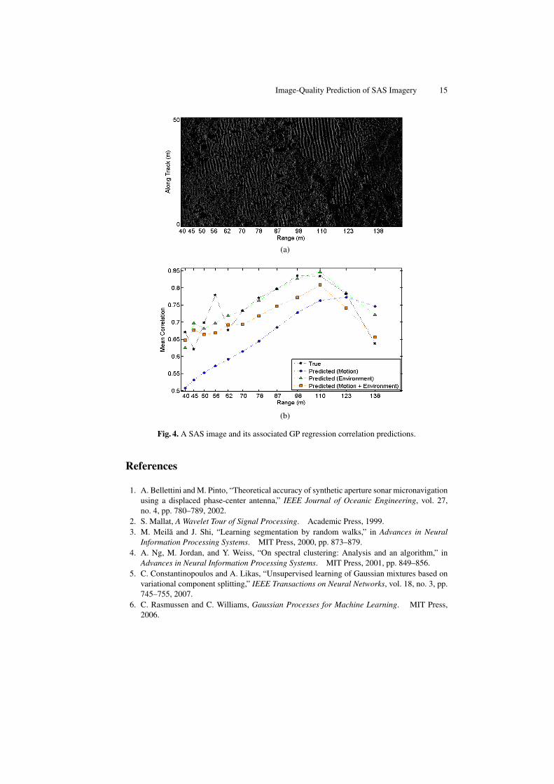
Image-Quality Prediction of SAS Imagery 15
(a)
(b)
Fig. 4. A SAS image and its associated GP regression correlation predictions.
References
1. A. Bellettini and M. Pinto, “Theoretical accuracy of synthetic aperture sonar micronavigationusing a displaced phase-center antenna,” IEEE Journal of Oceanic Engineering, vol. 27,no. 4, pp. 780–789, 2002.
2. S. Mallat, A Wavelet Tour of Signal Processing. Academic Press, 1999.3. M. Meila and J. Shi, “Learning segmentation by random walks,” in Advances in Neural
Information Processing Systems. MIT Press, 2000, pp. 873–879.4. A. Ng, M. Jordan, and Y. Weiss, “On spectral clustering: Analysis and an algorithm,” in
Advances in Neural Information Processing Systems. MIT Press, 2001, pp. 849–856.5. C. Constantinopoulos and A. Likas, “Unsupervised learning of Gaussian mixtures based on
variational component splitting,” IEEE Transactions on Neural Networks, vol. 18, no. 3, pp.745–755, 2007.
6. C. Rasmussen and C. Williams, Gaussian Processes for Machine Learning. MIT Press,2006.

16 David P. Williams
(a)
(b)
Fig. 5. A SAS image and its associated GP regression correlation predictions.
7. Y. Song, W. Chen, H. Bai, C. Lin, and E. Chang, “Parallel spectral clustering,” in Proceedingsof the European Conference on Machine Learning and Principles and Practice of KnowledgeDiscovery in Databases (ECML/PKDD), 2008.
8. Y. Bengio, J. Paiement, P. Vincent, O. Delalleau, N. Le Roux, and M. Ouimet, “Out-of-sample extensions for LLE, isomap, MDS, eigenmaps, and spectral clustering,” in Advancesin Neural Information Processing Systems. MIT Press, 2004, pp. 177–184.
9. M. Hayes and P. Gough, “Broad-band synthetic aperture sonar,” IEEE Journal of OceanicEngineering, vol. 17, no. 1, pp. 80–94, 1992.
10. L. Zelnik-Manor and P. Perona, “Self-tuning spectral clustering,” in Advances in NeuralInformation Processing Systems. MIT Press, 2004, pp. 1601–1608.
11. U. von Luxburg, “A tutorial on spectral clustering,” Statistics and Computing, vol. 17, no. 4,pp. 395–416, 2007.
12. M. Beal and Z. Ghahramani, “The variational Bayesian EM algorithm for incomplete data:Application to scoring graphical model structures,” Bayesian Statistics, vol. 7, pp. 453–464,2003.