1

Image Super-Resolution via Sparse RepresentationJianchao Yang,Student Member, IEEE, John Wright,Student Member, IEEE Thomas Huang,Life Fellow, IEEE

and Yi Ma, Senior Member, IEEE

Abstract—This paper presents a new approach to single-image superresolution, based on sparse signal representation.Research on image statistics suggests that image patches canbe well-represented as a sparse linear combination of elementsfrom an appropriately chosen over-complete dictionary. Inspiredby this observation, we seek a sparse representation for eachpatch of the low-resolution input, and then use the coefficientsof this representation to generate the high-resolution output.Theoretical results from compressed sensing suggest that undermild conditions, the sparse representation can be correctlyrecovered from the downsampled signals. By jointly training twodictionaries for the low resolution and high resolution imagepatches, we can enforce the similarity of sparse representationsbetween the low resolution and high resolution image patch pairwith respect to their own dictionaries. Therefore, the sparserepresentation of a low resolution image patch can be appliedwith the high resolution image patch dictionary to generateahigh resolution image patch. The learned dictionary pair is amore compact representation of the patch pairs, compared toprevious approaches which simply sample a large amount ofimage patch pairs, reducing the computational cost substantially.The effectiveness of such a sparsity prior is demonstrated forgeneral image super-resolution and also for the special case offace hallucination. In both cases, our algorithm generateshigh-resolution images that are competitive or even superior in qualityto images produced by other similar SR methods, but with fasterprocessing speed.

I. I NTRODUCTION

Super-resolution image reconstruction is currently a veryactive area of research, as it offers the promise of overcomingsome of the inherent resolution limitations of low-cost imagingsensors (e.g. cell phone or surveillance cameras) allowingbet-ter utilization of the growing capability of high-resolution dis-plays (e.g. high-definition LCDs). Such resolution-enhancingtechnology may also prove to be essential in medical imagingand satellite imaging where diagnosis or analysis from low-quality images can be extremely difficult. Conventional ap-proaches to generating a super-resolution (SR) image normallyrequire as inputmultiple low-resolution images of the samescene, which are aligned with sub-pixel accuracy. The SRtask is cast as the inverse problem of recovering the originalhigh-resolution image by fusing the low-resolution images,based on reasonable assumptions or prior knowledge aboutthe observation model that maps the high-resolution imageto the low-resolution images. The fundamental reconstructionconstraint for SR is that the recovered image, after applyingthe same generation model, should reproduce the observed low

Jianchao Yang and Thomas Huang are with Beckman Institute, Uni-versity of Illinois Urbana-Champaign, Urbana, IL 61801 USA(email:jyang29@ifp.uiuc.edu; huang@ifp.uiuc.edu).

John Wright and Yi Ma are with CSL, University of IllinoisUrbana-Champaign, Urbana, IL 61801 USA (email: jnwright@uiuc.edu;yima@uiuc.edu).

resolution images. However, SR image reconstruction is gen-erally a severely ill-posed problem because of the insufficientnumber of low resolution images, ill-conditioned registrationand unknown blurring operators, and the solution from thereconstruction constraint is not unique. Various regularizationmethods have been proposed to further stabilize the inversionthis ill-posed problem, such as [14], [11], [25].

However, the performance of these reconstruction-basedsuper-resolution algorithms degrades rapidly when the desiredmagnification factor is large or the number of available inputimages is small. In these cases, the result may be overlysmooth, lacking important high-frequency details [2]. Anotherclass of SR approach is based on interpolation [29], [6],[27]. While simple interpolation methods such as bilinear orbicubic interpolation tend to generate overly smooth imageswith ringing and jagged artifacts, interpolation by exploitingthe natural image priors will generally produce more favorableresults. Daiet al. [6] represented the local image patches usingthe background/foreground descriptors and reconstructedthesharp discontinuity between the two. Sunet. al. [27] exploredthe gradient profile prior for local image structures and ap-plied it to super-resolution. Such approaches are effective inpreserving the edges in the zoomed image. However, they arelimited in modeling the visual complexity of the real images.For natural images with fine textures or smooth shading, theseapproaches tend to produce watercolor-like artifacts.

A third category of SR approach is based on ma-chine learning techniques, which attempt to capture the co-occurrence prior between low-resolution and high-resolutionimage patches. [12] proposed an example-based learning strat-egy that applies to generic images where the low-resolutiontohigh-resolution prediction is learned via a Markov RandomField (MRF) solved by belief propagation. [23] extends thisapproach by using the Primal Sketch priors to enhance blurrededges, ridges and corners. Nevertheless, the above methodstypically require enormous databases of millions of high-resolution and low-resolution patch pairs, and are thereforecomputationally intensive. [5] adopts the philosophy of LLE[22] from manifold learning, assuming similarity betweenthe two manifolds in the high-resolution patch space andthe low-resolution patch space. Their algorithm maps thelocal geometry of the low-resolution patch space to the high-resolution patch space, generating high-resolution patchas alinear combination of neighbors. Using this strategy, morepatch patterns can be represented using a smaller trainingdatabase. However, using a fixed number K neighbors forreconstruction often results in blurring effects, due to over-or under-fitting.

While the mentioned approaches above were proposed forgeneric image super-resolution, specific image priors can be

2

incorporated when tailored to SR applications for specificdomains such as human faces. Thisface hallucination prob-lem was addressed in the pioneering work of Baker andKanade [30]. However, the gradient pyramid-based predictionintroduced in [30] does not directly model the face prior, andthe pixels are predicted individually, causing discontinuitiesand artifacts. Liuet al. [16] proposed a two-step statisticalapproach integrating the global PCA model and a local patchmodel. Although the algorithm yields good results, the holisticPCA model tends to yield results like the mean face and theprobabilistic local patch model is complicated and compu-tationally demanding. Wei Liuet al. [32] proposed a newapproach based on TensorPatches and residue compensation.While this algorithm adds more details to the face, it alsointroduces more artifacts.

This paper focuses on the problem of recovering the super-resolution version of a given low-resolution image. Similar tothe aforementioned learning-based methods, we will rely onpatches from the input image. However, instead of workingdirectly with the image patch pairs sampled from high res-olution and low resolution images [33], we learn a compactrepresentation for these patch pairs to capture the co-ocurrenceprior, significantly improving the speed of the algorithm.Our approach is motivated by recent results in sparse signalrepresentation, which suggest that the linear relationshipsamong high-resolution signals can be accurately recoveredfrom their low-dimensional projections [3], [9]. Althoughthesuper-resolution problem is very ill-posed, making preciserecovery impossible, the image patch sparse representationdemonstrates both effectiveness and robustness in regularizingthe inverse problem.

a) Basic Ideas: To be more precise, letD ∈ Rn×K be

an overcomplete dictionary ofK bases, and suppose a signalx ∈ R

n can be represented as a sparse linear combinationwith respect toD. That is, the signalx can be written asx = Dα0 where whereα0 ∈ R

K is a vector with very few(≪ K) nonzero entries. In practice, we might only observe asmall set of measurementsy of x:

y.= Lx = LDα0, (1)

whereL ∈ Rk×n with k < n is a projection matrix. In our

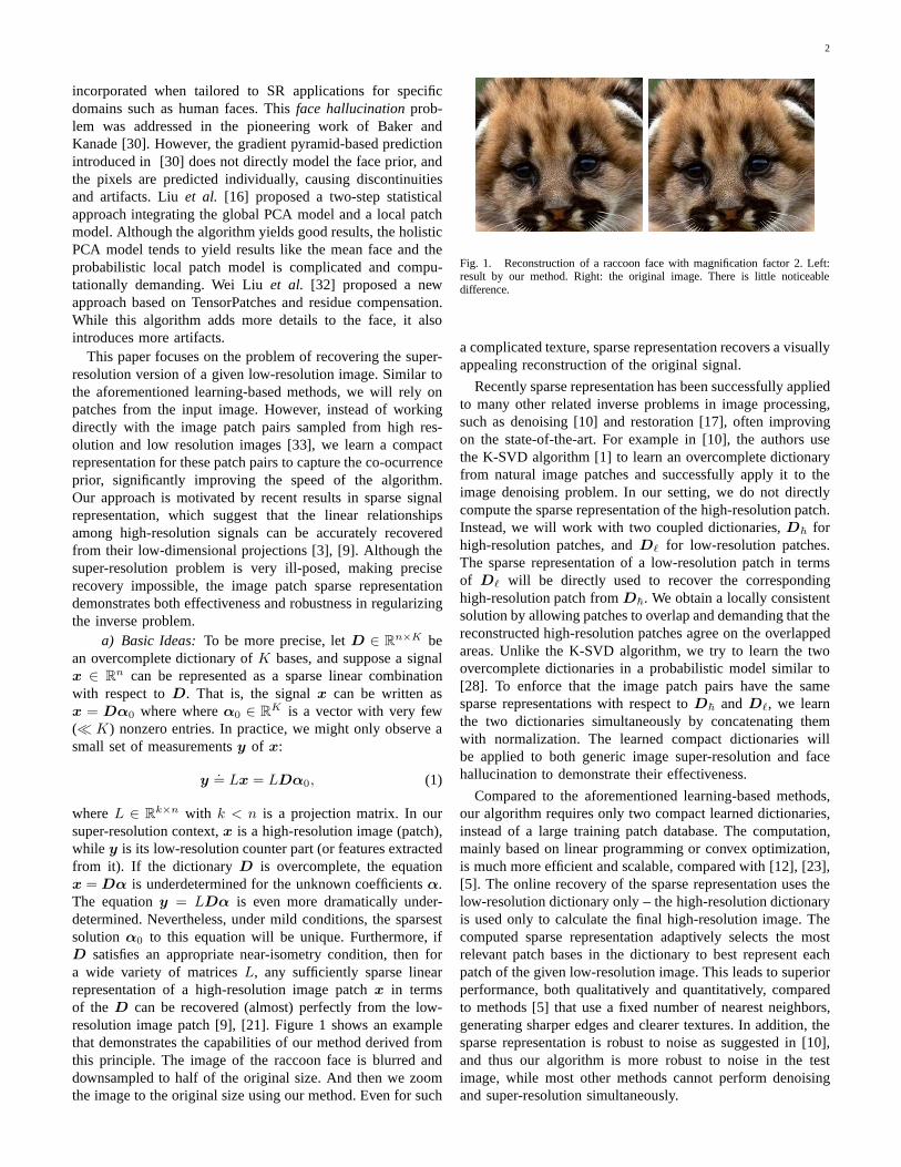
super-resolution context,x is a high-resolution image (patch),while y is its low-resolution counter part (or features extractedfrom it). If the dictionaryD is overcomplete, the equationx = Dα is underdetermined for the unknown coefficientsα.The equationy = LDα is even more dramatically under-determined. Nevertheless, under mild conditions, the sparsestsolution α0 to this equation will be unique. Furthermore, ifD satisfies an appropriate near-isometry condition, then fora wide variety of matricesL, any sufficiently sparse linearrepresentation of a high-resolution image patchx in termsof the D can be recovered (almost) perfectly from the low-resolution image patch [9], [21]. Figure 1 shows an examplethat demonstrates the capabilities of our method derived fromthis principle. The image of the raccoon face is blurred anddownsampled to half of the original size. And then we zoomthe image to the original size using our method. Even for such

Fig. 1. Reconstruction of a raccoon face with magnification factor 2. Left:result by our method. Right: the original image. There is little noticeabledifference.

a complicated texture, sparse representation recovers a visuallyappealing reconstruction of the original signal.

Recently sparse representation has been successfully appliedto many other related inverse problems in image processing,such as denoising [10] and restoration [17], often improvingon the state-of-the-art. For example in [10], the authors usethe K-SVD algorithm [1] to learn an overcomplete dictionaryfrom natural image patches and successfully apply it to theimage denoising problem. In our setting, we do not directlycompute the sparse representation of the high-resolution patch.Instead, we will work with two coupled dictionaries,D~ forhigh-resolution patches, andDℓ for low-resolution patches.The sparse representation of a low-resolution patch in termsof Dℓ will be directly used to recover the correspondinghigh-resolution patch fromD~. We obtain a locally consistentsolution by allowing patches to overlap and demanding that thereconstructed high-resolution patches agree on the overlappedareas. Unlike the K-SVD algorithm, we try to learn the twoovercomplete dictionaries in a probabilistic model similar to[28]. To enforce that the image patch pairs have the samesparse representations with respect toD~ and Dℓ, we learnthe two dictionaries simultaneously by concatenating themwith normalization. The learned compact dictionaries willbe applied to both generic image super-resolution and facehallucination to demonstrate their effectiveness.

Compared to the aforementioned learning-based methods,our algorithm requires only two compact learned dictionaries,instead of a large training patch database. The computation,mainly based on linear programming or convex optimization,is much more efficient and scalable, compared with [12], [23],[5]. The online recovery of the sparse representation uses thelow-resolution dictionary only – the high-resolution dictionaryis used only to calculate the final high-resolution image. Thecomputed sparse representation adaptively selects the mostrelevant patch bases in the dictionary to best represent eachpatch of the given low-resolution image. This leads to superiorperformance, both qualitatively and quantitatively, comparedto methods [5] that use a fixed number of nearest neighbors,generating sharper edges and clearer textures. In addition, thesparse representation is robust to noise as suggested in [10],and thus our algorithm is more robust to noise in the testimage, while most other methods cannot perform denoisingand super-resolution simultaneously.

3

b) Organization of the Paper: The remainder of thispaper is organized as follows. Section II details our formula-tion and solution to the image super-resolution problem basedon sparse representation. Specifically, we study how to applysparse representation for both generic image super-resolutionand face hallucination. In Section III, we discuss how to learnthe two dictionaries for the high-resolution and low-resolutionimage patches respectively. Various experimental resultsinSection IV demonstrate the efficacy of sparsity as a prior forregularizing image super-resolution.

c) Notations: Specifically X and Y denote the highresolution and low resolution image respectively, andx andy denote the high resolution and low resolution image patchrespectively. We use bold uppercaseD to denote the dictionaryfor sparse coding, especially we useD~ and Dℓ to denotethe dictionaries for high resolution and low resolution imagepatches respectively. Bold lowercase letters denote vectors.Unbold uppercase letters denote regular matrices, i.e.,D isused as a downsampling operation in matrix form. And unboldlowercase letters are used as scalars.

II. I MAGE SUPER-RESOLUTION FROMSPARSITY

The single-image super-resolution problem asks: given alow-resolution imageY , recover a higher-resolution imageXof the same scene. Two constraints are modeled in this work toregularize this ill-posed problem: 1) reconstruction constraint,which requires that the recoverdX should be consistent withthe input Y with respect to the image generation model;and 2) sparsity prior, which assumes that the high resolutionpatches can be sparsely represented in an appropriately chosenovercomplete dictionary, and that their sparse representationscan be recovered from the low resolution observation.

1) Reconstruction constraint: The observed low-resolutionimageY is a blurred and downsampled version of the highresolution imageX:

Y = DHX (2)

Here,H represents a blurring filter, andD the downsamplingoperator.

Super-resolution remains extremely ill-posed, since for agiven low-resolution inputY , infinitely many high-resolutionimages X satisfy the above reconstruction constraint. Wefurther regularize the problem via the following prior on smallpatchesx of X:

2) Sparsity prior: The patchesx of the high-resolutionimageX can be represented as a sparse linear combination ina dictionaryD~ trained from high-resolution patches sampledfrom training images:1

x ≈ D~α for someα ∈ RK with ‖α‖0 ≪ K. (3)

The sparse representationα will be recovered by representingpatchesy of the input imageY , with respect to a lowresolution dictionaryDℓ co-trained withD~. The dictionarytraining process will be discussed in Sec. III.

We apply our approach to both generic images and faceimages. For generic image super-resolution, we divide the

1Similar mechanisms – sparse coding with an overcomplete dictionary –are also believed to be employed by the human visual system [19].

problem into two steps. First, as suggested by the sparsityprior (3), we find the sparse representation for each localpatch, respecting spatial compatibility between neighbors.Next, using the result from this local sparse representation,we further regularize and refine the entire image using thereconstruction constraint (2). In this strategy, a local modelfrom the sparsity prior is used to recover lost high-frequencyfor local details. The global model from the reconstructionconstraint is then applied to remove possible artifacts fromthe first step and make the image more consistent and natural.The face images differ from the generic images in that the faceimages have more regular structure and thus reconstructionconstraints in the face subspace can be more effective. Forface image super-resolution, we reverse the above two stepsto make better use of the global face structure as a regularizer.We first find a suitable subspace for human faces, and applythe reconstruction constraints to recover a medium resolutionimage. We then recover the local details using the sparsityprior for image patches.

The remainder of this section is organized as follows: in Sec.II-A, we discuss super-resolution for generic images. We willintroduce the local model based on sparse representation andglobal model based on reconstruction constraints. In Sec. II-Bwe discuss how to introduce the global face structure into thisframework to achieve more accurate and visually appealingsuper-resolution for face images.

A. Generic Image Super-Resolution from Sparsity

1) Local model from sparse representation: Similar tothe patch-based methods mentioned previously, our algorithmtries to infer the high-resolution image patch for each low-resolution image patch from the input. For this local model,we have two dictionariesD~ and Dℓ, which are trained tohave the same sparse representations for each high-resolutionand low-resolution image patch pair. We subtract the meanpixel value for each patch, so that the dictionary representsimage textures rather than absolute intensities.

For each input low-resolution patchy, we find a sparserepresentation with respect toDℓ. The corresponding high-resolution patch basesD~ will be combined according to thesecoefficients to generate the output high-resolution patchx.The problem of finding the sparsest representation ofy canbe formulated as:

min ‖α‖0 s.t. ‖FDℓα− Fy‖22 ≤ ǫ, (4)

whereF is a (linear) feature extraction operator. The main roleof F in (4) is to provide a perceptually meaningful constraint2

on how closely the coefficientsα must approximatey. We willdiscuss the choice ofF in Section III.

Although the optimization problem (4) is NP-hard in gen-eral, recent results [7], [8] suggest that as long as the desiredcoefficientsα are sufficiently sparse, they can be efficientlyrecovered by instead minimizing theℓ1-norm, as follows:

min ‖α‖1 s.t. ‖FDℓα− Fy‖22 ≤ ǫ. (5)

2Traditionally, one would seek the sparsestα s.t. ‖Dℓα− y‖2 ≤ ǫ. Forsuper-resolution, it is more appropriate to replace this2-norm with a quadraticnorm ‖ · ‖

F T Fthat penalizes visually salient high-frequency errors.

4

Lagrange multipliers offer an equivalent formulation

min λ‖α‖1 + 1

2‖FDℓα− Fy‖22, (6)

where the parameterλ balances sparsity of the solutionand fidelity of the approximation toy. Notice that this isessentially a linear regression regularized withℓ1-norm on thecoefficients, known in statistical literature as the Lasso [24].

Solving (6) individually for each local patch does notguarantee the compatibility between adjacent patches. Weenforce compatibility between adjacent patches using a one-pass algorithm similar to that of [13].3 The patches areprocessed in raster-scan order in the image, from left to rightand top to bottom. We modify (5) so that the super-resolutionreconstructionD~α of patch y is constrained to closelyagree with the previously computed adjacent high-resolutionpatches. The resulting optimization problem is

min ‖α‖1 s.t. ‖FDℓα− Fy‖22 ≤ ǫ1,

‖PD~α−w‖22 ≤ ǫ2,(7)

where the matrixP extracts the region of overlap between cur-rent target patch and previously reconstructed high-resolutionimage, andw contains the values of the previously recon-structed high-resolution image on the overlap. The constrainedoptimization (7) can be similarly reformulated as:

min λ‖α‖1 + 1

2‖Dα− y‖22, (8)

where D =

[

FDℓ

βPD~

]

and y =

[

Fy

βw

]

. The parameterβ

controls the tradeoff between matching the low-resolutioninput and finding a high-resolution patch that is compatiblewith its neighbors. In all our experiments, we simply setβ = 1. Given the optimal solutionα∗ to (8), the high-resolution patch can be reconstructed asx = D~α∗.

2) Enforcing global reconstruction constraint: Notice that(5) and (7) do not demand exact equality between the low-resolution patchy and its reconstructionDℓα. Because ofthis, and also because of noise, the high-resolution imageX0 produced by the sparse representation approach of theprevious section may not satisfy the reconstruction constraint(2) exactly. We eliminate this discrepency by projectingX0

onto the solution space ofDHX = Y , computing

X∗ = argminX‖X −X0‖ s.t. DHX = Y . (9)

The solution to this optimization problem can be efficientlycomputed using the back-projection method, originally devel-oped in computer tomography and applied to super-resolutionin [15], [4]. The update equation for this iterative method is

Xt+1 = Xt + ((Y −DHXt) ↑ s) ∗ p, (10)

whereXt is the estimate of the high-resolution image afterthet-th iteration,p is a “backprojection” filter, and↑ s denotesupsampling by a factor ofs.

We take resultX∗ from backprojection as our final estimateof the high-resolution image. This image is as close as

3There are different ways to enforce compatibility. In [5], the values in theoverlapped regions are simply averaged, which will result in blurring effects.The one-pass algorithm [13] is shown to work almost as well asthe use of afull MRF model [12].

Algorithm 1 (Super-Resolution via Sparse Representation).1: Input: training dictionariesD~ andDℓ, a low-resolution

imageY .2: For each3 × 3 patch y of Y , taken starting from the

upper-left corner with1 pixel overlap in each direction,

• Solve the optimization problem withD andy definedin (8): min λ‖α‖1 + 1

2‖Dα− y‖22.

• Generate the high-resolution patchx = D~α∗. Putthe patchx into a high-resolution imageX0.

3: End4: Using back-projection, find the closest image toX0 which

satisfies the reconstruction constraint:

X∗ = arg minX‖X −X0‖ s.t. DHX = Y .

5: Output: super-resolution imageX∗.

possible to the initial super-resolutionX0 given by sparsity,while satisfying the reconstruction constraint. The entire super-resolution process is summarized as Algorithm 1.

3) Global optimization interpretation: The simple SR algo-rithm outlined in the previous two subsections can be viewedas a special case of a more general sparse representationframework for inverse problems in image processing. Relatedideas have been profitably applied in image compression,denoising [10], and restoration [17]. In addition to placingour work in a larger context, these connections suggest meansof further improving the performance, at the cost of increasedcomputational complexity.

Given sufficient computational resources, one could in prin-ciple solve for the coefficients associated with all patchessimultaneously. Moreover, the entire high-resolution imageX

itself can be treated as a variable. Rather than demanding thatX be perfectly reproduced by the sparse coefficientsα, wecan penalize the difference betweenX and the high-resolutionimage given by these coefficients, allowing solutions thatare not perfectly sparse, but better satisfy the reconstructionconstraints. This leads to a large optimization problem:

X∗ = arg minX,αij

‖DHX − Y ‖22 + η∑

i,j

‖αij‖0

+ γ∑

i,j

‖D~αij − PijX‖22 + τρ(X)

.(11)

Here, αij denotes the representation coefficients for the(i, j)th patch ofX , andPij is a projection matrix that selectsthe (i, j)th patch fromX. ρ(X) is a penalty function thatencodes prior knowledge about the high-resolution image. Thisfunction may depend on the image category, or may take theform of a generic regularization term (e.g., Huber MRF, TotalVariation, Bilateral Total Variation).

Algorithm 1 can be interpreted as a computationally efficientapproximation to (11). The sparse representation step recoversthe coefficientsα by approximately minimizing the sum ofthe second and third terms of (11). The sparsity term‖αij‖0is relaxed to‖αij‖1, while the high-resolution fidelity term‖D~αij − PijX‖2 is approximated by its low-resolution

5

version‖FDℓαij − Fyij‖2.Notice, that if the sparse coefficientsα are fixed, the third

term of (11) essentially penalizes the difference between thesuper-resolution imageX and the reconstruction given bythe coefficients:

∑

i,j ‖D~αij − PijX‖22 ≈ ‖X0 − X‖22.

Hence, for smallγ, the back-projection step of Algorithm 1approximately minimizes the sum of the first and third termsof (11).

Algorithm 1 does not, however, incorporate any prior be-sides sparsity of the representation coefficients – the termρ(X) is absent in our approximation. In Section IV we willsee that sparsity in a relevant dictionary is a strong enoughprior that we can already achieve good super-resolution per-formance. Nevertheless, in settings where further assumptionson the high-resolution signal are available, these priors canbe incorperated into the global reconstruction step of ouralgorithm.

B. Face super-resolution from Sparsity

Face resolution enhancement is usually desirable in manysurveillance scenarios, where there is always a large distancebetween the camera and the objects (people) of interest.Unlike the generic image super-resolution discussed earlier,face images are more regular and thus should be easier tohandle. Indeed, for face super-resolution, we can deal withlower resolution input images. The basic idea is first to usethe face prior to zoom the image to a reasonable mediumresolution, and then to employ the local sparsity prior modelto recover details. To be more precise, the solution is alsoapproached in two steps: 1) global model: use reconstructionconstraint to recover a medium high-resolution face image,but the solution is searched only in the face subspace; and 2)local model: use the local sparse model to recover the imagedetails.

a) Non-negative matrix factorization: In face super-resolution, the most frequently used subspace method for mod-eling the human face is Principal Component Analysis (PCA),which chooses a low-dimensional subspace that captures asmuch of the variance as possible. However, the PCA basesare holistic, and tend to generate smooth faces similar to themean. Moreover, because principal component representationsallow negative coefficients, the PCA reconstruction is oftenhard to interpret.

Even though faces are objects with lots of variance, theyare made up of several relatively independent parts such aseyes, eyebrows, noses, mouths, checks and chins. NonnegativeMatrix Factorization (NMF) [31] seeks a representation of thegiven signals as an additive combination of local features.Tofind such a part-based subspace, NMF is formulated as thefollowing optimization problem:

arg minU,V‖Z − UV ‖22

s.t. U ≥ 0, V ≥ 0,(12)

whereZ ∈ Rn×m is the data matrix,U ∈ R

n×r is the basismatrix andV ∈ R

r×m is the coefficient matrix. In our contexthere,A simply consists of a set of high-resolution training faceimages as its column vectors. The number of the basesr can

be chosen asn ∗m/(n + m) which is smaller thann andm,meaning a more compact representation. It can be shown thata locally optimum of (12) can be obtained via the followingupdate rules:

Vij ←− Vij

(UT Z)ij

(UT UV )ij

Uki ←− Uki

(ZV T )ki

(UV V T )ki

,

(13)

where1 ≤ i ≤ r, 1 ≤ j ≤ m and 1 ≤ k ≤ n. The obtainedbasis matrixU is often sparse and localized.

b) Two step face super-resolution: Let X andY denotethe high resolution and low resolution faces respectively.Y isobtained fromX by smoothing and downsampling as in Eq.2, GivenY , we can achieve the optimal solution forX basedon the Maximuma Posteriori (MAP) criteria,

X∗ = arg maxX

p(Y |X)p(X). (14)

Using the rules in (13), we can obtain the basis matrixU , which is composed of sparse bases. LetΩ denote theface subspace spanned byU . Then in the subspaceΩ, thesuper-resolution problem in (14) can be formulated using thereconstruction constraints as:

c∗ = argminc‖DHUc− Y ‖22 + λρ(Uc) s.t. c ≥ 0,

(15)

whereρ(Uc) is a prior term regularizing the high resolutionsolution,c ∈ R

r×1 is the coefficient vector in the subspaceΩfor estimated the high resolution face, andλ is a parameterused to balance the reconstruction fidelity and the penalty ofthe prior term. In this paper, we simply use a generic imageprior requiring that the solution be smooth. LetΓ denote amatrix performing high-pass filtering. The final formulationfor (15) is:

c∗ = argminc‖DHUc− Y ‖22 + λ‖ΓUc‖2 s.t. c ≥ 0.

(16)

The medium high-resolution imageX is approximated byUc∗. The prior term in (16) suppresses the high frequencycomponents, resulting in over-smoothness in the solutionimage. We rectify this using the local patch model basedon sparse representation mentioned earlier in Sec. II-A1.The complete framework of our algorithm is summarized asAlgorithm 2.

III. L EARNING THE DICTIONARY PAIR

In the previous section, we discussed regularizing the super-resolution problem using sparse prior that each pair of high-and low-resolution image patches have the same sparse rep-resentations with respect to the two dictionariesD~ andDℓ. A straightforward way to obtain two such dictionariesis to sample image patch pairs directly, which preserves thecorrespondence between the high resolution and low resolutionpatch items [33]. However, such a strategy will result in largedictionaries and hence expensive computation. This sectionwill focus on learning a more compact dictionary pair forspeeding up the computation.

6

Algorithm 2 (Face Hallucination via Sparse Representation).1: Input: sparse basis matrixU , training dictionariesD~ and

Dℓ, a low-resolution imageY .2: Find a smooth high-resolution faceX from the subspace

spanned byU through:

• Solve the optimization problem in (16):arg minc ‖MUc− Y ‖2 + λ‖ΓUc‖2 s.t. c ≥ 0.

• X = Uc∗.

3: For each patchy of X, taken starting from the upper-leftcorner with1 pixel overlap in each direction,

• Solve the optimization problem withD andy definedin (8): min η‖α‖1 + 1

2‖Dα− y‖22.

• Generate the high-resolution patchx = D~α∗. Putthe patchx into a high-resolution imageX∗.

4: Output: super-resolution faceX∗.

A. Single Dictionary Training

Sparse coding is the problem of learning a dictionaryD

that can sparsely represent a given set of training examplesX = x1, x2, ..., xt. Generally, it is hard to learn a compactdictionary which guarantees that sparse representation of(4)can be recovered fromℓ1 minimization in (5). Fortunately,many sparse coding algorithms proposed previously suffice forpractical applications. In this work, we focus on the followingformulation:

D =arg minD,Z‖X −DZ‖22 + λ‖Z‖1

s.t. ‖Di‖22 ≤ 1, i = 1, 2, ..., K.

(17)

where theℓ1 norm‖Z‖1 is to enforce sparsity, and theℓ2 normconstraints on each columns remove the scaling ambiguity4.This particular formulation has been studied extensively [19],[28], [34]. (17) is not convex in bothD andZ, but is convex inone of them with the other fixed. The basic idea is to minimize(17) alternatively over the codesZ for a given dictionaryD,and then overD for a givenZ, leading to a local minimumof the overall objective function.

B. Joint Dictionary Training

Given the sampled training image patch pairsP =Xh, Y l, whereXh = x1, x2, ..., xn are the set of sampledhigh resolution image patches andY l = y1, y2, ..., yn arethe corresponding low resolution image patches (or features),our goal is to learn dictionaries for high resolution and lowres-olution image patches, so that the sparse representation ofthehigh resolution patch is the same as the sparse representationof the corresponding low resolution patch. This is a difficultproblem, due to the ill-posed nature of super-resolution. Theindividual sparse coding problems in the high-resolution andlow-resolution patch spaces are

D~ = arg minDh,Z

‖Xh −DhZ‖22 + λ‖Z‖1, (18)

4Note that without the norm constraints the cost can always bereduced bydividing Z by c > 1 and multiplyingD by c > 1.

andDℓ = arg min

Dl,Z‖Y l −DlZ‖22 + λ‖Z‖1, (19)

respectively. We combine these objectives, forcing the high-resolution and low-resolution representations to share the samecodes, instead writing

minDh,Dl,Z

1

N‖Xh −DhZ‖22 +

1

M‖Y l −DlZ‖22

+ λ(1

N+

1

M)‖Z‖1,

(20)

whereN andM are the dimensions of the high resolution andlow resolution image patches in vector form. Here,1/N and1/M balance the two cost terms of (18) and (19). (20) can berewritten as

minDh,Dl,Z

‖Xc −DcZ‖22 + λ(

1

N+

1

M)‖Z‖1, (21)

or equivalently

minDh,Dl,Z

‖Xc −DcZ‖22 + λ‖Z‖1, (22)

where

Xc =

[

1√N

Xh

1√M

Y l

]

, Dc =

[

1√N

D~

1√M

Dℓ

]

. (23)

Thus we can use the same learning strategy in the singledictionary case for training the two dictionaries for our super-resolution purpose. Note that since we are using features fromthe low resolution image patches,Dh andDl are not simplyconnected by a linear transform, otherwise the training processof (22) will depend on the high resolution image patches only(for detail, refer to Part III-C). Fig. 2 shows the dictionarylearned by (22) for generic images.5 The learned dictionarydemonstrates basic patterns of the image patches, such asorientated edges, instead of raw patch prototypes, due to itscompactness.

C. Feature Representation for Low Resolution Image Patches

In (4), we use a feature transformationF to ensure that thecomputed coefficients fit the most relevant part of the low-resolution signal, and hence have a more accurate predictionfor the high resolution image patch reconstruction. Typically,F is chosen as some kind of high-pass filter. This is reasonablefrom a perceptual viewpoint, since people are more sensitive tothe high-frequency content of the image. The high-frequencycomponents of the low-resolution image are also arguably themost important for predicting the lost high-frequency contentin the target high-resolution image.

In the literature, people have suggested extracting differentfeatures for the low resolution image patch in order to boostthe prediction accuracy. Freeman et al. [12] used a high-passfilter to extract the edge information from the low-resolutioninput patches as the feature. Sun et. al. [23] used a set ofGaussian derivative filters to extract the contours in the low-resolution patches. Chang et. al. [5] used the first-order and

5We omit the dictionary for the low resolution image patches because weare training on features instead the patches themselves.

7

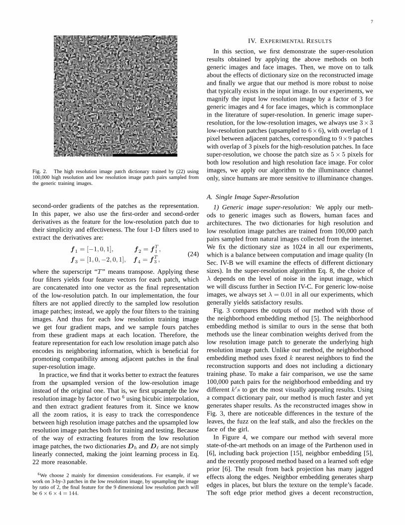
Fig. 2. The high resolution image patch dictionary trained by (22) using100,000 high resolution and low resolution image patch pairs sampled fromthe generic training images.

second-order gradients of the patches as the representation.In this paper, we also use the first-order and second-orderderivatives as the feature for the low-resolution patch duetotheir simplicity and effectiveness. The four 1-D filters used toextract the derivatives are:

f1 = [−1, 0, 1], f2 = fT1 ,

f3 = [1, 0,−2, 0, 1], f4 = fT3 ,

(24)

where the superscript “T ” means transpose. Applying thesefour filters yields four feature vectors for each patch, whichare concatenated into one vector as the final representationof the low-resolution patch. In our implementation, the fourfilters are not applied directly to the sampled low resolutionimage patches; instead, we apply the four filters to the trainingimages. And thus for each low resolution training imagewe get four gradient maps, and we sample fours patchesfrom these gradient maps at each location. Therefore, thefeature representation for each low resolution image patchalsoencodes its neighboring information, which is beneficial forpromoting compatibility among adjacent patches in the finalsuper-resolution image.

In practice, we find that it works better to extract the featuresfrom the upsampled version of the low-resolution imageinstead of the original one. That is, we first upsample the lowresolution image by factor of two6 using bicubic interpolation,and then extract gradient features from it. Since we knowall the zoom ratios, it is easy to track the correspondencebetween high resolution image patches and the upsampled lowresolution image patches both for training and testing. Becauseof the way of extracting features from the low resolutionimage patches, the two dictionariesD~ andDℓ are not simplylinearly connected, making the joint learning process in Eq.22 more reasonable.

6We choose 2 mainly for dimension considerations. For example, if wework on 3-by-3 patches in the low resolution image, by upsampling the imageby ratio of 2, the final feature for the 9 dimensional low resolution patch willbe 6 × 6 × 4 = 144.

IV. EXPERIMENTAL RESULTS

In this section, we first demonstrate the super-resolutionresults obtained by applying the above methods on bothgeneric images and face images. Then, we move on to talkabout the effects of dictionary size on the reconstructed imageand finally we argue that our method is more robust to noisethat typically exists in the input image. In our experiments, wemagnify the input low resolution image by a factor of 3 forgeneric images and 4 for face images, which is commonplacein the literature of super-resolution. In generic image super-resolution, for the low-resolution images, we always use3×3low-resolution patches (upsampled to6×6), with overlap of 1pixel between adjacent patches, corresponding to9×9 patcheswith overlap of 3 pixels for the high-resolution patches. Infacesuper-resolution, we choose the patch size as5× 5 pixels forboth low resolution and high resolution face image. For colorimages, we apply our algorithm to the illuminance channelonly, since humans are more sensitive to illuminance changes.

A. Single Image Super-Resolution

1) Generic image super-resolution: We apply our meth-ods to generic images such as flowers, human faces andarchitectures. The two dictionaries for high resolution andlow resolution image patches are trained from 100,000 patchpairs sampled from natural images collected from the internet.We fix the dictionary size as 1024 in all our experiments,which is a balance between computation and image quality (InSec. IV-B we will examine the effects of different dictionarysizes). In the super-resolution algorithm Eq. 8, the choiceofλ depends on the level of noise in the input image, whichwe will discuss further in Section IV-C. For generic low-noiseimages, we always setλ = 0.01 in all our experiments, whichgenerally yields satisfactory results.

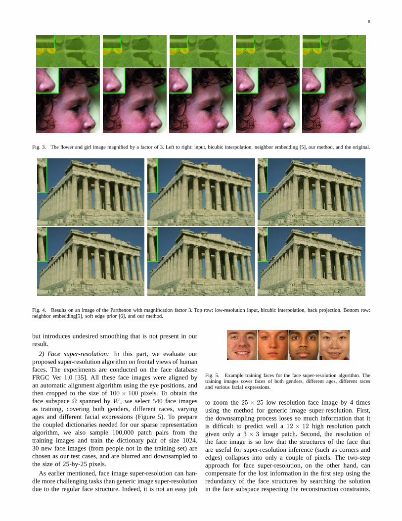
Fig. 3 compares the outputs of our method with those ofthe neighborhood embedding method [5]. The neighborhoodembedding method is similar to ours in the sense that bothmethods use the linear combination weights derived from thelow resolution image patch to generate the underlying highresolution image patch. Unlike our method, the neighborhoodembedding method uses fixedk nearest neighbors to find thereconstruction supports and does not including a dictionarytraining phase. To make a fair comparison, we use the same100,000 patch pairs for the neighborhood embedding and trydifferentk′s to get the most visually appealing results. Usinga compact dictionary pair, our method is much faster and yetgenerates shaper results. As the reconstructed images showinFig. 3, there are noticeable differences in the texture of theleaves, the fuzz on the leaf stalk, and also the freckles on theface of the girl.

In Figure 4, we compare our method with several morestate-of-the-art methods on an image of the Parthenon used in[6], including back projection [15], neighbor embedding [5],and the recently proposed method based on a learned soft edgeprior [6]. The result from back projection has many jaggedeffects along the edges. Neighbor embedding generates sharpedges in places, but blurs the texture on the temple’s facade.The soft edge prior method gives a decent reconstruction,

8

Fig. 3. The flower and girl image magnified by a factor of 3. Leftto right: input, bicubic interpolation, neighbor embedding [5], our method, and the original.

Fig. 4. Results on an image of the Parthenon with magnification factor 3. Top row: low-resolution input, bicubic interpolation, back projection. Bottom row:neighbor embedding[5], soft edge prior [6], and our method.

but introduces undesired smoothing that is not present in ourresult.

2) Face super-resolution: In this part, we evaluate ourproposed super-resolution algorithm on frontal views of humanfaces. The experiments are conducted on the face databaseFRGC Ver 1.0 [35]. All these face images were aligned byan automatic alignment algorithm using the eye positions, andthen cropped to the size of100 × 100 pixels. To obtain theface subspaceΩ spanned byW , we select 540 face imagesas training, covering both genders, different races, varyingages and different facial expressions (Figure 5). To preparethe coupled dictionaries needed for our sparse representationalgorithm, we also sample 100,000 patch pairs from thetraining images and train the dictionary pair of size 1024.30 new face images (from people not in the training set) arechosen as our test cases, and are blurred and downsampled tothe size of 25-by-25 pixels.

As earlier mentioned, face image super-resolution can han-dle more challenging tasks than generic image super-resolutiondue to the regular face structure. Indeed, it is not an easy job

Fig. 5. Example training faces for the face super-resolution algorithm. Thetraining images cover faces of both genders, different ages, different racesand various facial expressions.

to zoom the25 × 25 low resolution face image by 4 timesusing the method for generic image super-resolution. First,the downsampling process loses so much information that itis difficult to predict well a12 × 12 high resolution patchgiven only a3 × 3 image patch. Second, the resolution ofthe face image is so low that the structures of the face thatare useful for super-resolution inference (such as cornersandedges) collapses into only a couple of pixels. The two-stepapproach for face super-resolution, on the other hand, cancompensate for the lost information in the first step using theredundancy of the face structures by searching the solutionin the face subspace respecting the reconstruction constraints.

9

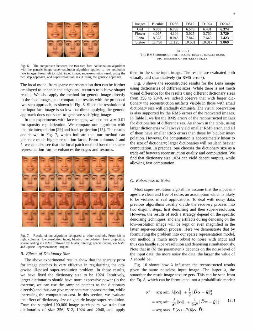
Fig. 6. The comparison between the two-step face hallucination algorithmwith the generic image super-resolution algorithm appliedto low resolutionface images. From left to right: input image, super-resolution result using thetwo step approach, and super-resolution result using the generic approach.

The local model from sparse representation then can be furtheremployed to enhance the edges and textures to achieve shaperresults. We also apply the method for generic image directlyto the face images, and compare the results with the proposedtwo-step approach, as shown in Fig. 6. Since the resolution ofthe input face image is so low that direct applying the genericapproach does not seem to generate satisfying image.

In our experiments with face images, we also setλ = 0.01for sparsity regularization. We compare our algorithm withbicubic interpolation [29] and back-projection [15]. The resultsare shown in Fig. 7, which indicate that our method cangenerate much higher resolution faces. From columns 4 and5, we can also see that the local patch method based on sparserepresentation further enhances the edges and textures.

Fig. 7. Results of our algorithm compared to other methods. From left toright columns: low resolution input; bicubic interpolation; back projection;sparse coding via NMF followed by bilater filtering; sparse coding via NMFand Sparse Representation; Original.

B. Effects of Dictionary Size

The above experimental results show that the sparsity priorfor image patches is very effective in regularizing the oth-erwise ill-posed super-resolution problem. In those results,we have fixed the dictionary size to be 1024. Intuitively,larger dictionaries should have more expressive power (in theextreme, we can use the sampled patches as the dictionarydirectly) and thus can give more accurate approximation, whileincreasing the computation cost. In this section, we evaluatethe effect of dictionary size on generic image super-resolution.From the sampled 100,000 image patch pairs, we train fourdictionaries of size 256, 512, 1024 and 2048, and apply

Images Bicubic D256 D512 D1024 D2048

Girl 6.858 6.739 6.579 6.431 6.374Flower 4.097 4.104 3.925 3.760 3.720Lena 8.578 8.043 7.842 7.645 7.423Statue 11.490 11.125 10.601 10.017 9.869

TABLE ITHE RMS ERRORS OF THE RECONSTRUCTED IMAGES USING

DICTIONARIES OF DIFFERENT SIZES.

them to the same input image. The results are evaluated bothvisually and quantitatively (in RMS errors).

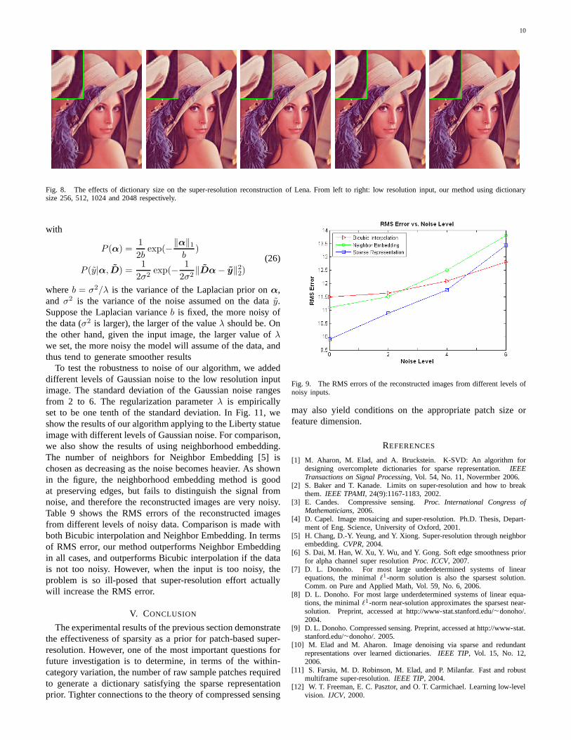
Fig. 8 shows the reconstructed results for the Lena imageusing dictionaries of different sizes. While there is not muchvisual difference for the results using different dictionary sizesfrom 256 to 2048, we indeed observe that with larger dic-tionary the reconstruction artifacts visible in those withsmalldictionary size will gradually diminish. The visual observationis also supported by the RMS errors of the recovered images.In Table I, we list the RMS errors of the reconstructed imagesfor dictionaries of different sizes. As shown in the table, usinglarger dictionaries will always yield smaller RMS error, and allof them have smaller RMS errors than those by bicubic inter-polation. However, the computation is approximately linear tothe size of dictionary; larger dictionaries will result in heaviercomputation. In practice, one chooses the dictionary size as atrade-off between reconstruction quality and computation. Wefind that dictionary size 1024 can yield decent outputs, whileallowing fast computation.

C. Robustness to Noise

Most super-resolution algorithms assume that the input im-ages are clean and free of noise, an assumption which is likelyto be violated in real applications. To deal with noisy data,previous algorithms usually divide the recovery process intotwo disjoint steps: first denoising and then super-resolution.However, the results of such a strategy depend on the specificdenoising techniques, and any artifacts during denosing onthelow-resolution image will be kept or even magnified in thelatter super-resolution process. Here we demonstrate thatbyformulating the problem into our sparse representation model,our method is much more robust to noise with input andthus can handle super-resolution and denoising simultaneously.Note that in (6) the parameterλ depends on the noise level ofthe input data; the more noisy the data, the larger the value ofλ should be.

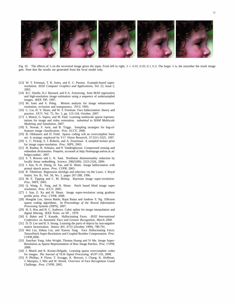
Fig. 10 shows howλ influence the reconstructed resultsgiven the same noiseless input image. The largerλ, thesmoother the result image texture gets. This can be seen fromthe Eq. 8, which can be formulated into a probabilistic model:

α∗ = arg min λ‖α‖1 +1

2‖Dα− y‖22

= arg minλ

σ2‖α‖1 +

1

2σ2‖Dα− y‖22

= arg max P (α) · P (y|α, D)

(25)

10

Fig. 8. The effects of dictionary size on the super-resolution reconstruction of Lena. From left to right: low resolution input, our method using dictionarysize 256, 512, 1024 and 2048 respectively.

with

P (α) =1

2bexp(−

‖α‖1b

)

P (y|α, D) =1

2σ2exp(−

1

2σ2‖Dα− y‖22)

(26)

whereb = σ2/λ is the variance of the Laplacian prior onα,and σ2 is the variance of the noise assumed on the datay.Suppose the Laplacian varianceb is fixed, the more noisy ofthe data (σ2 is larger), the larger of the valueλ should be. Onthe other hand, given the input image, the larger value ofλwe set, the more noisy the model will assume of the data, andthus tend to generate smoother results

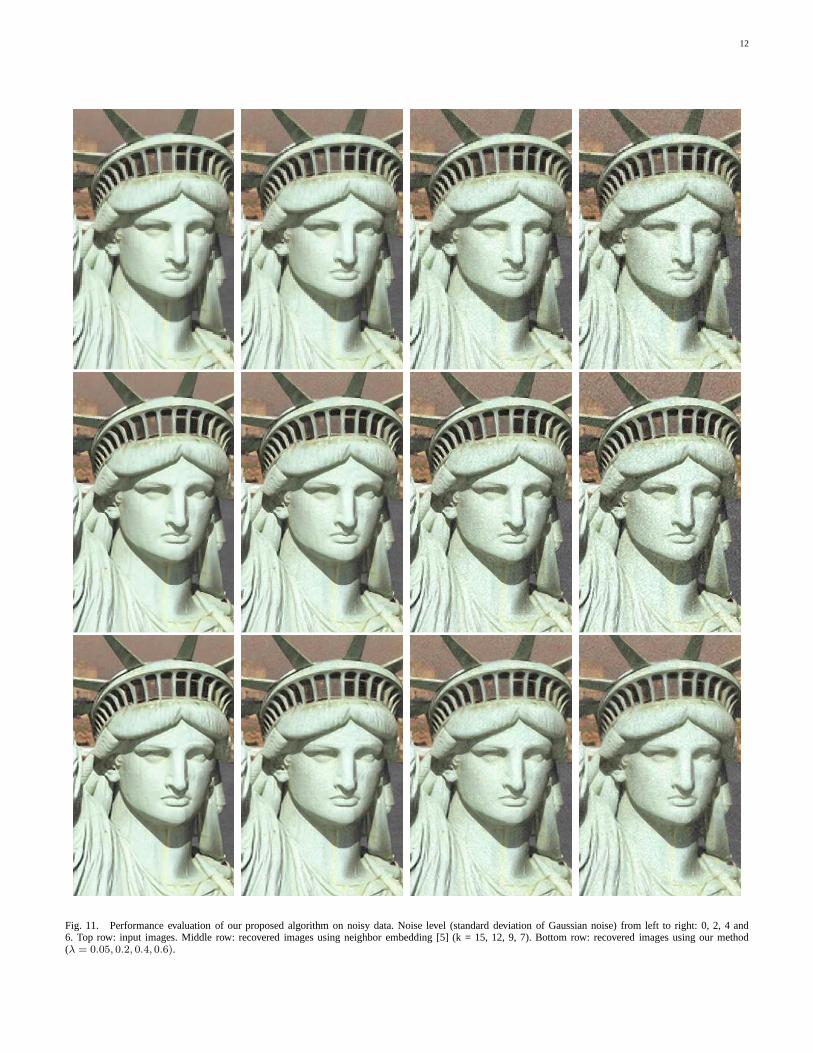
To test the robustness to noise of our algorithm, we addeddifferent levels of Gaussian noise to the low resolution inputimage. The standard deviation of the Gaussian noise rangesfrom 2 to 6. The regularization parameterλ is empiricallyset to be one tenth of the standard deviation. In Fig. 11, weshow the results of our algorithm applying to the Liberty statueimage with different levels of Gaussian noise. For comparison,we also show the results of using neighborhood embedding.The number of neighbors for Neighbor Embedding [5] ischosen as decreasing as the noise becomes heavier. As shownin the figure, the neighborhood embedding method is goodat preserving edges, but fails to distinguish the signal fromnoise, and therefore the reconstructed images are very noisy.Table 9 shows the RMS errors of the reconstructed imagesfrom different levels of noisy data. Comparison is made withboth Bicubic interpolation and Neighbor Embedding. In termsof RMS error, our method outperforms Neighbor Embeddingin all cases, and outperforms Bicubic interpolation if the datais not too noisy. However, when the input is too noisy, theproblem is so ill-posed that super-resolution effort actuallywill increase the RMS error.

V. CONCLUSION

The experimental results of the previous section demonstratethe effectiveness of sparsity as a prior for patch-based super-resolution. However, one of the most important questions forfuture investigation is to determine, in terms of the within-category variation, the number of raw sample patches requiredto generate a dictionary satisfying the sparse representationprior. Tighter connections to the theory of compressed sensing

Fig. 9. The RMS errors of the reconstructed images from different levels ofnoisy inputs.

may also yield conditions on the appropriate patch size orfeature dimension.

REFERENCES

[1] M. Aharon, M. Elad, and A. Bruckstein. K-SVD: An algorithm fordesigning overcomplete dictionaries for sparse representation. IEEETransactions on Signal Processing, Vol. 54, No. 11, Novermber 2006.

[2] S. Baker and T. Kanade. Limits on super-resolution and how to breakthem. IEEE TPAMI, 24(9):1167-1183, 2002.

[3] E. Candes. Compressive sensing.Proc. International Congress ofMathematicians, 2006.

[4] D. Capel. Image mosaicing and super-resolution. Ph.D. Thesis, Depart-ment of Eng. Science, University of Oxford, 2001.

[5] H. Chang, D.-Y. Yeung, and Y. Xiong. Super-resolution through neighborembedding.CVPR, 2004.

[6] S. Dai, M. Han, W. Xu, Y. Wu, and Y. Gong. Soft edge smoothness priorfor alpha channel super resolutionProc. ICCV, 2007.

[7] D. L. Donoho. For most large underdetermined systems of linearequations, the minimalℓ1-norm solution is also the sparsest solution.Comm. on Pure and Applied Math, Vol. 59, No. 6, 2006.

[8] D. L. Donoho. For most large underdetermined systems of linear equa-tions, the minimalℓ1-norm near-solution approximates the sparsest near-solution. Preprint, accessed at http://www-stat.stanford.edu/∼donoho/.2004.

[9] D. L. Donoho. Compressed sensing. Preprint, accessed athttp://www-stat.stanford.edu/∼donoho/. 2005.

[10] M. Elad and M. Aharon. Image denoising via sparse and redundantrepresentations over learned dictionaries.IEEE TIP, Vol. 15, No. 12,2006.

[11] S. Farsiu, M. D. Robinson, M. Elad, and P. Milanfar. Fastand robustmultiframe super-resolution.IEEE TIP, 2004.

[12] W. T. Freeman, E. C. Pasztor, and O. T. Carmichael. Learning low-levelvision. IJCV, 2000.

11

Fig. 10. The effects ofλ on the recovered image given the input. From left to right,λ = 0.01, 0.05, 0.1, 0.3. The largerλ is, the smoother the result imagegets. Note that the results are generated from the local model only.

[13] W. T. Freeman, T. R. Jones, and E. C. Pasztor. Example-based super-resolution. IEEE Computer Graphics and Applications, Vol. 22, Issue 2,2002.

[14] R.C. Hardie, K.J. Barnard, and E.A. Armstrong. Joint MAP registrationand high-resolution image estimation using a sequence of undersampledimages.IEEE TIP, 1997.

[15] M. Irani and S. Peleg. Motion analysis for image enhancement:resolution, occlusion and transparency.JVCI, 1993.

[16] C. Liu, H. Y. Shum, and W. T. Freeman. Face hallucination: theory andpractice. IJCV, Vol. 75, No. 1, pp. 115-134, October, 2007.

[17] J. Mairal, G. Sapiro, and M. Elad. Learning multiscale sparse represen-tations for image and video restoration.submitted to SIAM MultiscaleModeling and Simulation, 2007.

[18] E. Nowak, F. Jurie, and B. Triggs. Sampling strategies for bag-of-features image classification.Proc. ECCV, 2006.

[19] B. Olshausen and D. Field. Sparse coding wih an overcomplete basisset: A strategy employed by V1?Vision Research, 37:3311-3325, 1997.

[20] L. C. Pickup, S. J. Roberts, and A. Zisserman. A sampled texture priorfor image super-resolution.Proc. NIPS, 2003.

[21] H. Rauhut, K. Schnass, and P. Vandergheynst. Compressed sensing andredundant dictionaries. Preprint, accessed at http://homepage.univie.ac.at/holger.rauhut/. 2007.

[22] S. T. Roweis and L. K. Saul. Nonlinear dimensionality reduction bylocally linear embedding.Science, 290(5500): 2323-2326, 2000.

[23] J. Sun, N.-N. Zheng, H. Tao, and H. Shum. Image hallucination withprimal sketch priors.Proc. CVPR, 2003.

[24] R. Tibshirani. Regression shrinkge and selection via the Lasso. J. RoyalStatist. Soc B., Vol. 58, No. 1, pages 267-288, 1996.

[25] M. E. Tipping and C. M. Bishop. Bayesian image super-resolution.Proc. NIPS, 2003.

[26] Q. Wang, X. Tang, and H. Shum. Patch based blind image superresolution. Proc. ICCV, 2005.

[27] J. Sun, Z. Xu and H. Shum. Image super-resolution using gradientprofile prior. Proc. CVPR, 2008.

[28] Honglak Lee, Alexis Battle, Rajat Raina and Andrew Y. Ng. Efficientsparse coding algorithms. InProceedings of the Neural InformationProcessing Systems (NIPS), 2007.

[29] H. S. Hou and H. C. Andrews. Cubic spline for image interpolation anddigital filtering. IEEE Trans. on SP, , 1978.

[30] S. Baker and T. Kanade. Hallucinating Faces.IEEE InternationalConference on Automatic Face and Gesture Recognition, March 2000.

[31] D. D. Lee and H. S. Seung. Learning the parts of objects bynon-negativematrix factorization.Nature 401, 6755 (October 1999), 788-791.

[32] Wei Liu, Dahua Lin, and Xiaoou Tang. Face HallucinatingFaces:TensorPatch Super-Resolution and Coupled Residue Compensation. Proc.CVPR,2006.

[33] Jianchao Yang, John Wright, Thomas Huang and Yi Ma. Image Super-Resolution as Sparse Representation of Raw Image Patches.Proc. CVPR,2008.

[34] J. Mutch and K. Kreutz-Delgado. Learning sparse overcomplete codesfor images.The Journal of VLSI Signal Processing, 45:97-110, 2008.

[35] P. Phillips, P. Flynn, T. Scruggs, K. Bowyer, J. Chang, K. Hoffman,J. Marques, J. Min and W. Worek. Overview of Face RecognitionGrandChallenge.Proc. CVPR, 2005.

12

Fig. 11. Performance evaluation of our proposed algorithm on noisy data. Noise level (standard deviation of Gaussian noise) from left to right: 0, 2, 4 and6. Top row: input images. Middle row: recovered images usingneighbor embedding [5] (k = 15, 12, 9, 7). Bottom row: recovered images using our method(λ = 0.05, 0.2, 0.4, 0.6).