1

Image Deblurring and Super-resolution by Adaptive Sparse Domain Selection and Adaptive Regularization

Weisheng Donga,b, Lei Zhangb,1, Member, IEEE,

Guangming Shia, Senior Member, IEEE, and Xiaolin Wuc, Senior Member, IEEE

aKey Laboratory of Intelligent Perception and Image Understanding (Chinese Ministry of Education),

School of Electronic Engineering, Xidian University, China bDept. of Computing, The Hong Kong Polytechnic University, Hong Kong

cDept. of Electrical and Computer Engineering, McMaster University, Canada Abstract: As a powerful statistical image modeling technique, sparse representation has been successfully

used in various image restoration applications. The success of sparse representation owes to the development

of l1-norm optimization techniques, and the fact that natural images are intrinsically sparse in some domain.

The image restoration quality largely depends on whether the employed sparse domain can represent well

the underlying image. Considering that the contents can vary significantly across different images or

different patches in a single image, we propose to learn various sets of bases from a pre-collected dataset of

example image patches, and then for a given patch to be processed, one set of bases are adaptively selected

to characterize the local sparse domain. We further introduce two adaptive regularization terms into the

sparse representation framework. First, a set of autoregressive (AR) models are learned from the dataset of

example image patches. The best fitted AR models to a given patch are adaptively selected to regularize the

image local structures. Second, the image non-local self-similarity is introduced as another regularization

term. In addition, the sparsity regularization parameter is adaptively estimated for better image restoration

performance. Extensive experiments on image deblurring and super-resolution validate that by using

adaptive sparse domain selection and adaptive regularization, the proposed method achieves much better

results than many state-of-the-art algorithms in terms of both PSNR and visual perception.

Key Words: Sparse representation, image restoration, deblurring, super-resolution, regularization.

1 Corresponding author: cslzhang@comp.polyu.edu.hk. This work is supported by the Hong Kong RGC General

Research Fund (PolyU 5375/09E).

2

I. Introduction

Image restoration (IR) aims to reconstruct a high quality image x from its degraded measurement y. IR is a

typical ill-posed inverse problem [1] and it can be generally modeled as

y=DHx+υ, (1)

where x is the unknown image to be estimated, H and D are degrading operators and υ is additive noise.

When H and D are identities, the IR problem becomes denoising; when D is identity and H is a blurring

operator, IR becomes deblurring; when D is identity and H is a set of random projections, IR becomes

compressed sensing [2-4]; when D is a down-sampling operator and H is a blurring operator, IR becomes

(single image) super-resolution. As a fundamental problem in image processing, IR has been extensively

studied in the past three decades [5-20]. In this paper, we focus on deblurring and single image

super-resolution.

Due to the ill-posed nature of IR, the solution to Eq. (1) with an l2-norm fidelity constraint, i.e.,

2

2ˆ arg min= −

xx y DHx , is generally not unique. To find a better solution, prior knowledge of natural images

can be used to regularize the IR problem. One of the most commonly used regularization models is the total

variation (TV) model [6-7]: { }2

2 1ˆ arg min +λ= − ⋅ ∇

xx y DHx x , where |∇x|1 is the l1-norm of the first order

derivative of x and λ is a constant. Since the TV model favors the piecewise constant image structures, it

tends to smooth out the fine details of an image. To better preserve the image edges, many algorithms have

been later developed to improve the TV models [17-19, 42, 45, 47].

The success of TV regularization validates the importance of good image prior models in solving the IR

problems. In wavelet based image denoising [21], researchers have found that the sparsity of wavelet

coefficients can serve as good prior. This reveals the fact that many types of signals, e.g., natural images, can

be sparsely represented (or coded) using a dictionary of atoms, such as DCT or wavelet bases. That is,

denote by Φ the dictionary, we have x≈Φα and most of the coefficients in α are close to zero. With the

sparsity prior, the representation of x over Φ can be estimated from its observation y by solving the

following l0-minimization problem: { }2

2 0ˆ arg min +λ= − ⋅y DHΦα α

αα , where the l0-norm counts the

number of nonzero coefficients in vector α. Once α̂ is obtained, x can then be estimated as ˆ ˆ=x Φα . The

3

l0-minimization is an NP-hard combinatorial search problem, and is usually solved by greedy algorithms [48,

60]. The l1-minimization, as the closest convex function to l0-minimization, is then widely used as an

alternative approach to solving the sparse coding problem: { }2

2 1ˆ arg min +λ= − ⋅y DHΦα α

αα [60]. In

addition, recent studies showed that iteratively reweighting the l1-norm sparsity regularization term can lead

to better IR results [59]. Sparse representation has been successfully used in various image processing

applications [2-4, 13, 21-25, 32].

A critical issue in sparse representation modeling is the determination of dictionary Φ. Analytically

designed dictionaries, such as DCT, wavelet, curvelet and contourlets, share the advantages of fast

implementation; however, they lack the adaptivity to image local structures. Recently, there has been much

effort in learning dictionaries from example image patches [13-15, 26-31, 55], leading to state-of-the-art

results in image denoising and reconstruction. Many dictionary learning (DL) methods aim at learning a

universal and over-complete dictionary to represent various image structures. However, sparse

decomposition over a highly redundant dictionary is potentially unstable and tends to generate visual

artifacts [53-54]. In this paper we propose an adaptive sparse domain selection (ASDS) scheme for sparse

representation. By learning a set of compact sub-dictionaries from high quality example image patches. The

example image patches are clustered into many clusters. Since each cluster consists of many patches with

similar patterns, a compact sub-dictionary can be learned for each cluster. Particularly, for simplicity we use

the principal component analysis (PCA) technique to learn the sub-dictionaries. For an image patch to be

coded, the best sub-dictionary that is most relevant to the given patch is selected. Since the given patch can

be better represented by the adaptively selected sub-dictionary, the whole image can be more accurately

reconstructed than using a universal dictionary, which will be validated by our experiments.

Apart from the sparsity regularization, other regularization terms can also be introduced to further

increase the IR performance. In this paper, we propose to use the piecewise autoregressive (AR) models,

which are pre-learned from the training dataset, to characterize the local image structures. For each given

local patch, one or several AR models can be adaptively selected to regularize the solution space. On the

other hand, considering the fact that there are often many repetitive image structures in an image, we

introduce a non-local (NL) self-similarity constraint served as another regularization term, which is very

helpful in preserving edge sharpness and suppressing noise.

4

After introducing ASDS and adaptive regularizations (AReg) into the sparse representation based IR

framework, we present an efficient iterative shrinkage (IS) algorithm to solve the l1-minimization problem.

In addition, we adaptively estimate the image local sparsity to adjust the sparsity regularization parameters.

Extensive experiments on image deblurring and super-resolution show that the proposed ASDS-AReg

approach can effectively reconstruct the image details, outperforming many state-of-the-art IR methods in

terms of both PSNR and visual perception.

The rest of the paper is organized as follows. Section II introduces the related works. Section III presents

the ASDS-based sparse representation. Section IV describes the AReg modeling. Section V summarizes the

proposed algorithm. Section VI presents experimental results and Section VII concludes the paper.

II. Related Works

It has been found that natural images can be generally coded by structural primitives, e.g., edges and line

segments [61], and these primitives are qualitatively similar in form to simple cell receptive fields [62]. In

[63], Olshausen et al. proposed to represent a natural image using a small number of basis functions chosen

out of an over-complete code set. In recent years, such a sparse coding or sparse representation strategy has

been widely studied to solve inverse problems, partially due to the progress of l0-norm and l1-norm

minimization techniques [60].

Suppose that x∈ℜn is the target signal to be coded, and Φ =[φ1,…, φm]∈ℜn×m is a given dictionary of

atoms (i.e., code set). The sparse coding of x over Φ is to find a sparse vector α=[α1;…;αm] (i.e., most of the

coefficients in α are close to zero) such that x≈Φα [49]. If the sparsity is measured as the l0-norm of α,

which counts the non-zero coefficients in α, the sparse coding problem becomes 2

2min −α

x Φα s.t.0

T≤α ,

where T is a scalar controlling the sparsity [55]. Alternatively, the sparse vector α can also be found by

{ }2

2 0ˆ arg min +λ= − ⋅x

αα Φα α , (2)

where λ is a constant. Since the l0-norm is non-convex, it is often replaced by either the standard l1-norm or

the weighted l1-norm to make the optimization problem convex [3, 57, 59, 60].

An important issue of the sparse representation modeling is the choice of dictionary Φ. Much effort has

been made in learning a redundant dictionary from a set of example image patches [13-15, 26-31, 55]. Given

5

a set of training image patches S=[s1, …, sN]∈ℜn×N, the goal of dictionary learning (DL) is to jointly

optimize the dictionary Φ and the representation coefficient matrix Λ=[α1,…,αN] such that i i≈s αΦ and

i pT≤α , where p = 0 or 1. This can be formulated by the following minimization problem:

2ˆˆ( ) arg minF

=Φ,Λ

Φ,Λ S -ΦΛ s.t. ,i pT i≤ ∀α , (3)

where ||·||F is the Frobenius norm. The above minimization problem is non-convex even when p=1. To make

it tractable, approximation approaches, including MOD [56] and K-SVD [26], have been proposed to

alternatively optimizing Φ and Λ, leading to many state-of-the-art results in image processing [14-15, 31].

Various extensions and variants of the K-SVD algorithm [27, 29-31] have been proposed to learn a

universal and over-complete dictionary. However, the image contents can vary significantly across images.

One may argue that a well learned over-complete dictionary Φ can sparsely code all the possible image

structures; nonetheless, for each given image patch, such a “universal” dictionary Φ is neither optimal nor

efficient because many atoms in Φ are irrelevant to the given local patch. These irrelevant atoms will not

only reduce the computational efficiency in sparse coding but also reduce the representation accuracy.

Regularization has been used in IR for a long time to incorporate the image prior information. The

widely used TV regularizations lack flexibilities in characterizing the local image structures and often

generate over-smoothed results. As a classic method, the autoregressive (AR) modeling has been

successfully used in image compression [33] and interpolation [34-35]. Recently the AR model was used for

adaptive regularization in compressive image recovery [40]: 2

2min s.t. i i i

ix − =∑x

α y Axχ , where χi is

the vector containing the neighboring pixels of pixel xi within the support of the AR model, and ai is the AR

parameter vector. In [40], the AR models are locally computed from an initially recovered image, and they

perform much better than the TV regularization in reconstructing the edge structures. However, the AR

models estimated from the initially recovered image may not be robust and tend to produce the “ghost”

visual artifacts. In this paper, we will propose a learning-based adaptive regularization, where the AR models

are learned from high-quality training images, to increase the AR modeling accuracy.

In recent years the non-local (NL) methods have led to promising results in various IR tasks, especially

in image denoising [36, 15, 39]. The mathematical framework of NL means filtering was well established by

Buades et al. [36]. The idea of NL methods is very simple: the patches that have similar patterns can be

6

spatially far from each other and thus we can collect them in the whole image. This NL self-similarity prior

was later employed in image deblurring [8, 20] and super-resolution [41]. In [15], the NL self-similarity

prior was combined with the sparse representation modeling, where the similar image patches are

simultaneously coded to improve the robustness of inverse reconstruction. In this work, we will also

introduce an NL self-similarity regularization term into our proposed IR framework.

III. Sparse Representation with Adaptive Sparse Domain Selection

In this section we propose an adaptive sparse domain selection (ASDS) scheme, which learns a series of

compact sub-dictionaries and assigns adaptively each local patch a sub-dictionary as the sparse domain.

With ASDS, a weighted l1-norm sparse representation model will be proposed for IR tasks. Suppose that

{Φk}, k=1,2,…,K, is a set of K orthonormal sub-dictionaries. Let x be an image vector, and xi=Rix,

i=1,2,…,N, be the ith patch (size: n n× ) vector of x, where Ri is a matrix extracting patch xi from x. For

patch xi, suppose that a sub-dictionary ikΦ is selected for it. Then, xi can be approximated as

1ˆ ,

ii k i i T= ≤x Φ α α , via sparse coding. The whole image x can be reconstructed by averaging all the

reconstructed patches ˆ ix , which can be mathematically written as [22]

( )1

1 1

ˆi

N NT Ti i i k i

i i

−

= =

⎛ ⎞= ⎜ ⎟⎝ ⎠∑ ∑x R R R Φ α . (4)

In Eq. (4), the matrix to be inverted is a diagonal matrix, and hence the calculation of Eq. (4) can be done in

a pixel-by-pixel manner [22]. Obviously, the image patches can be overlapped to better suppress noise [22,

15] and block artifacts. For the convenience of expression, we define the following operator “ο”:

( )1

1 1

ˆi

N NT Ti i i k i

i i

−

= =

⎛ ⎞= ⎜ ⎟

⎝ ⎠∑ ∑x R R RΦ α Φ α , (5)

where Φ is the concatenation of all sub-dictionaries {Φk} and α is the concatenation of all αi.

Let = +y DHx v be the observed degraded image, our goal is to recover the original image x from y.

With ASDS and the definition in Eq. (5), the IR problem can be formulated as follows:

{ }2

2 1ˆ arg min +λ= −y DH

αα Φ α α . (6)

Clearly, one key procedure in the proposed ASDS scheme is the determination of ikΦ for each local patch.

7

To facilitate the sparsity-based IR, we propose to learn offline the sub-dictionaries {Φk}, and select online

from {Φk} the best fitted sub-dictionary to each patch xi.

A. Learning the sub-dictionaries

In order to learn a series of sub-dictionaries to code the various local image structures, we need to first

construct a dataset of local image patches for training. To this end, we collected a set of high-quality natural

images, and cropped from them a rich amount of image patches with size n n× . A cropped image patch,

denoted by si, will be involved in DL if its intensity variance Var(si) is greater than a threshold Δ, i.e.,

Var(si)> Δ. This patch selection criterion is to exclude the smooth patches from training and guarantee that

only the meaningful patches with a certain amount of edge structures are involved in DL.

Suppose that M image patches S=[s1, s2, …, sM] are selected. We aim to learn K compact sub-dictionaries

{Φk} from S so that for each given local image patch, the most suitable sub-dictionary can be selected. To

this end, we cluster the dataset S into K clusters, and learn a sub-dictionary from each of the K clusters.

Apparently, the K clusters are expected to represent the K distinctive patterns in S. To generate perceptually

meaningful clusters, we perform the clustering in a feature space. In the hundreds of thousands patches

cropped from the training images, many patches are approximately the rotated version of the others. Hence

we do not need to explicitly make the training dataset invariant to rotation because it is naturally (nearly)

rotation invariant. Considering the fact that human visual system is sensitive to image edges, which convey

most of the semantic information of an image, we use the high-pass filtering output of each patch as the

feature for clustering. It allows us to focus on the edges and structures of image patches, and helps to

increase the accuracy of clustering. The high-pass filtering is often used in low-level statistical learning tasks

to enhance the meaningful features [50].

Denote by 1 2[ , ,..., ]h h hh M=S s s s the high-pass filtered dataset of S. We adopt the K-means algorithm to

partition Sh into K clusters 1 2{ , , , }KC C C and denote by μk the centroid of cluster Ck. Once Sh is

partitioned, dataset S can then be clustered into K subsets Sk, k=1,2,..,K, and Sk is a matrix of dimension

n×mk, where mk denotes the number of samples in Sk.

Now the remaining problem is how to learn a sub-dictionary Φk from the cluster Sk such that all the

elements in Sk can be faithfully represented by Φk. Meanwhile, we hope that the representation of Sk over Φk

8

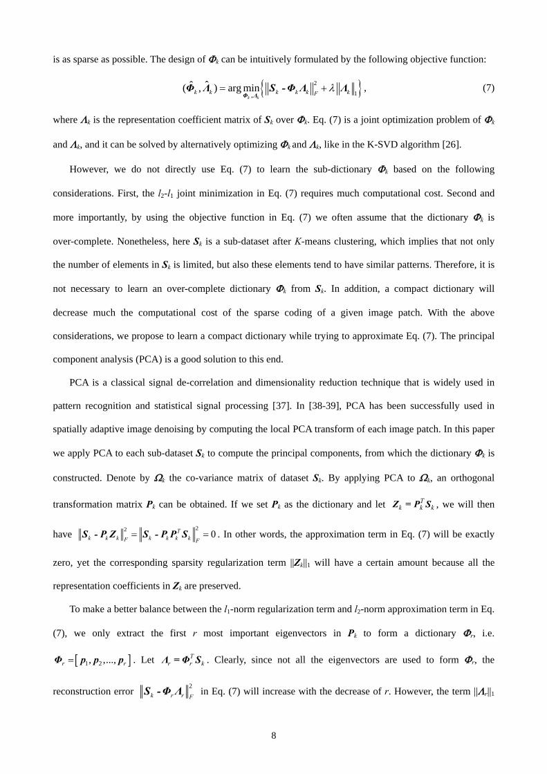
is as sparse as possible. The design of Φk can be intuitively formulated by the following objective function:

{ }2

1ˆˆ( , ) arg min

k kk k k k k kF

λ= +Φ ,Λ

Φ Λ S -Φ Λ Λ , (7)

where Λk is the representation coefficient matrix of Sk over Φk. Eq. (7) is a joint optimization problem of Φk

and Λk, and it can be solved by alternatively optimizing Φk and Λk, like in the K-SVD algorithm [26].

However, we do not directly use Eq. (7) to learn the sub-dictionary Φk based on the following

considerations. First, the l2-l1 joint minimization in Eq. (7) requires much computational cost. Second and

more importantly, by using the objective function in Eq. (7) we often assume that the dictionary Φk is

over-complete. Nonetheless, here Sk is a sub-dataset after K-means clustering, which implies that not only

the number of elements in Sk is limited, but also these elements tend to have similar patterns. Therefore, it is

not necessary to learn an over-complete dictionary Φk from Sk. In addition, a compact dictionary will

decrease much the computational cost of the sparse coding of a given image patch. With the above

considerations, we propose to learn a compact dictionary while trying to approximate Eq. (7). The principal

component analysis (PCA) is a good solution to this end.

PCA is a classical signal de-correlation and dimensionality reduction technique that is widely used in

pattern recognition and statistical signal processing [37]. In [38-39], PCA has been successfully used in

spatially adaptive image denoising by computing the local PCA transform of each image patch. In this paper

we apply PCA to each sub-dataset Sk to compute the principal components, from which the dictionary Φk is

constructed. Denote by Ωk the co-variance matrix of dataset Sk. By applying PCA to Ωk, an orthogonal

transformation matrix Pk can be obtained. If we set Pk as the dictionary and let Tk k kZ = Ρ S , we will then

have 22 0T

k k k k k k kF F= =S - P Z S - P P S . In other words, the approximation term in Eq. (7) will be exactly

zero, yet the corresponding sparsity regularization term ||Zk||1 will have a certain amount because all the

representation coefficients in Zk are preserved.

To make a better balance between the l1-norm regularization term and l2-norm approximation term in Eq.

(7), we only extract the first r most important eigenvectors in Pk to form a dictionary Φr, i.e.

[ ]1 2, ,...,r r=Φ p p p . Let Tr r kΛ = Φ S . Clearly, since not all the eigenvectors are used to form Φr, the

reconstruction error 2k r r F

S -Φ Λ in Eq. (7) will increase with the decrease of r. However, the term ||Λr||1

9

will decrease. Therefore, the optimal value of r, denoted by ro, can be determined by

{ }2

1arg mino k r r rFr

r λ= +S -Φ Λ Λ . (8)

Finally, the sub-dictionary learned from sub-dataset Sk is 1 2, ,...,ok r⎡ ⎤= ⎣ ⎦Φ p p p .

Applying the above procedures to all the K sub-datasets Sk, we could get K sub-dictionaries Φk, which

will be used in the adaptive sparse domain selection process of each given image patch. In Fig. 1, we show

some example sub-dictionaries learned from a training dataset. The left column shows the centroids of some

sub-datasets after K-means clustering, and the right eight columns show the first eight atoms in the

sub-dictionaries learned from the corresponding sub-datasets.

Fig. 1. Examples of learned sub-dictionaries. The left column shows the centriods of some sub-datasets after K-means clustering, and the right eight columns show the first eight atoms of the learned sub-dictionaries from the corresponding sub-datasets.

B. Adaptive selection of the sub-dictionary

In the previous subsection, we have learned a dictionary Φk for each subset Sk. Meanwhile, we have

computed the centroid μk of each cluster Ck associated with Sk. Therefore, we have K pairs {Φk, μk}, with

which the ASDS of each given image patch can be accomplished.

In the proposed sparsity-based IR scheme, we assign adaptively a sub-dictionary to each local patch of x,

spanning the adaptive sparse domain. Since x is unknown beforehand, we need to have an initial estimation

of it. The initial estimation of x can be accomplished by taking wavelet bases as the dictionary and then

solving Eq. (6) with the iterated shrinkage algorithm in [10]. Denote by x̂ the estimate of x, and denote by

ˆ ix a local patch of x̂ . Recall that we have the centroid μk of each cluster available, and hence we could

select the best fitted sub-dictionary to ˆ ix by comparing the high-pass filtered patch of ˆ ix , denoted by ˆ hix ,

10

to the centroid μk. For example, we can select the dictionary for ˆ ix based on the minimum distance

between ˆ hix and μk, i.e.

2ˆarg min h

i i kkk = −x μ . (9)

However, directly calculating the distance between ˆ hix and μk may not be robust enough because the

initial estimate x̂ can be noisy. Here we propose to determine the sub-dictionary in the subspace of μk. Let

[ ]1 2, ,..., K=U μ μ μ be the matrix containing all the centroids. By applying SVD to the co-variance matrix of

U, we can obtain the PCA transformation matrix of U. Let Φc be the projection matrix composed by the first

several most significant eigenvectors. We compute the distance between ˆ hix and μk in the subspace spanned

by Φc:

2ˆarg min h

i c i c kkk = −Φ x Φ μ . (10)

Compared with Eq. (9), Eq. (10) can increase the robustness of adaptive dictionary selection.

By using Eq. (10), the kith sub-dictionary

ikΦ will be selected and assigned to patch ˆ ix . Then we can

update the estimation of x by minimizing Eq. (6) and letting ˆ =x ˆΦ α . With the updated estimate x̂ , the

ASDS of x can be consequently updated. Such a process is iteratively implemented until the estimation x̂

converges.

C. Adaptively reweighted sparsity regularization

In Eq. (6), the parameter λ is a constant to weight the l1-norm sparsity regularization term 1

α . In [59]

Candes et al. showed that the reweighted l1-norm sparsity can more closely resemble the l0-norm sparsity

than using a constant weight, and consequently improve the reconstruction of sparse signals. In this

sub-section, we propose a new method to estimate adaptively the image local sparsity, and then reweight the

l1-norm sparsity in the ASDS scheme.

The reweighted l1-norm sparsity regularized minimization with ASDS can be formulated as follows:

2, ,2

1 1

ˆ arg min +N n

i j i ji j

λ α= =

⎧ ⎫= −⎨ ⎬

⎩ ⎭∑∑y DH

αα Φ α , (11)

where αi,j is the coefficient associated with the jth atom of ikΦ and λi,j is the weight assigned to αi,j. In [59],

11

λi,j is empirically computed as , ,ˆ1/(| | )i j i jλ α ε= + , where ,ˆi jα is the estimate of αi,j and ε is a small

constant. Here, we propose a more robust method for computing λi,j by formulating the sparsity estimation

as a Maximum a Posterior (MAP) estimation problem. Under the Bayesian framework, with the observation

y the MAP estimation of α is given by

{ } { }ˆ arg max log ( | ) arg min log ( | ) log ( )P P P= = − −y yαα

α α α α . (12)

By assuming y is contaminated with additive Gaussian white noises of standard deviation σn, we have:

22 2

1 1( | ) exp( )22 nn

Pσσ π

= − −y y DHα Φ α . (13)

The prior distribution P(α) is often characterized by an i.i.d. zero-mean Laplacian probability model:

,1 1,,

1 2( ) exp( )2

N ni ji j

i ji j

P ασσ= =

= −∏ ∏α , (14)

where σi,j is the standard deviation of αi,j. By plugging P(y|α) and P(α) into Eq. (12), we could readily derive

the desired weight in Eq. (11) as 2, ,2 2 /i j n i jλ σ σ= . For numerical stability, we compute the weights by

2

,,

2 2ˆ

ni j

i j

σλ

σ ε=

+, (15)

where ,ˆi jσ is an estimate of σi,j and ε is a small constant.

Now let’s discuss how to estimate σi,j. Denote by ˆ ix the estimate of ix , and by ˆ lix , l=1,2,…, L, the

non-local similar patches to ˆ ix . (The determination of non-local similar patches to ˆ ix will be described in

Section IV-C.) The representation coefficients of these similar patches over the selected sub-dictionary ikΦ

is ˆ ˆi

l T li k i= xα Φ . Then we can estimate σi,j by calculating the standard deviation of each element ,ˆi jα in ˆ l

iα .

Compared with the reweighting method in [59], the proposed adaptive reweighting method is more robust

because it exploits the image nonlocal redundancy information. Based on our experimental experience, it

could lead to about 0.2dB improvement in average over the reweighting method in [59] for deblurring and

super-resolution under the proposed ASDS framework. The detailed algorithm to solve the reweighted

l1-norm sparsity regularized minimization in Eq. (11) will be presented in Section V.

12

IV. Spatially Adaptive Regularization

In Section III, we proposed to select adaptively a sub-dictionary to code the given image patch. The

proposed ASDS-based IR method can be further improved by introducing two types of adaptive

regularization (AReg) terms. A local area in a natural image can be viewed as a stationary process, which

can be well modeled by the autoregressive (AR) models. Here, we propose to learn a set of AR models from

the clustered high quality training image patches, and adaptively select one AR model to regularize the input

image patch. Besides the AR models, which exploit the image local correlation, we propose to use the

non-local similarity constraint as a complementary AReg term to the local AR models. With the fact that

there are often many repetitive image structures in natural images, the image non-local redundancies can be

very helpful in image enhancement.

A. Training the AR models

Recall that in Section III, we have partitioned the whole training dataset into K sub-datasets Sk. For each Sk

an AR model can be trained using all the sample patches inside it. Here we let the support of the AR model

be a square window, and the AR model aims to predict the central pixel of the window by using the

neighboring pixels. Considering that determining the best order of the AR model is not trivial, and a high

order AR model may cause data over-fitting, in our experiments a 3×3 window (i.e., AR model of order 8) is

used. The vector of AR model parameters, denoted by ak, of the kth sub-dataset Sk, can be easily computed by

solving the following least square problem:

2arg min ( )i k

Tk i is

∈

= −∑as S

a a q , (16)

where si is the central pixel of image patch si and qi is the vector that consists of the neighboring pixels of si

within the support of the AR model. By applying the AR model training process to each sub-dataset, we can

obtain a set of AR models {a1, a2, …, aK} that will be used for adaptive regularization.

B. Adaptive selection of the AR model for regularization

The adaptive selection of the AR model for each patch xi is the same as the selection of sub-dictionary for xi

described in Section III-B. With an estimation ˆ ix of xi, we compute its high-pass Gaussian filtering output

13

ˆ hix . Let

2ˆarg min h

i c i c kkk = −Φ x Φ μ , and then the ki

th AR model ika will be assigned to patch xi. Denote by xi

the central pixel of patch xi, and by χi the vector containing the neighboring pixels of xi within patch xi. We

can expect that the prediction error of xi using ika and χi should be small, i.e.,

2

2i

Ti k ix − a χ should be

minimized. By incorporating this constraint into the ASDS based sparse representation model in Eq. (11), we

have a lifted objective function as follows:

22, ,2 2

1 1

ˆ arg min +i

i

N nT

i j i j i k ii j x

xλ α γ= = ∈

⎧ ⎫⎪ ⎪= − + ⋅ −⎨ ⎬⎪ ⎪⎩ ⎭

∑∑ ∑x

α y DHΦ α a χα

, (17)

where γ is a constant balancing the contribution of the AR regularization term. For the convenience of

expression, we write the third term 2

2i

i

Ti k i

x

x∈

−∑x

a χ as 2

2( )I - A x , where I is the identity matrix and

, if is an element of , ( , )

0, otherwiseii j i i ka x a

i j∈⎧⎪= ⎨

⎪⎩

χ aA .

Then, Eq. (17) can be rewritten as

2 2, ,2 2

1 1

ˆ arg min + ( )N n

i j i ji j

λ α γ= =

⎧ ⎫= − + ⋅ −⎨ ⎬

⎩ ⎭∑∑α y DHΦ α I A x

α. (18)

C. Adaptive regularization by non-local similarity

The AR model based AReg exploits the local statistics in each image patch. On the other hand, there are

often many repetitive patterns throughout a natural image. Such non-local redundancy is very helpful to

improve the quality of reconstructed images. As a complementary AReg term to AR models, we further

introduce a non-local similarity regularization term into the sparsity-based IR framework.

For each local patch xi, we search for the similar patches to it in the whole image x (in practice, in a

large enough area around xi). A patch lix is selected as a similar patch to xi if l

ie = ˆ|| ix 22ˆ ||l

i t− ≤x , where t

is a preset threshold, and ˆ ix and ˆ lix are the current estimates of xi and l

ix , respectively. Or we can select

the patch ˆ lix if it is within the first L (L=10 in our experiments) closest patches to ˆ ix . Let xi be the central

pixel of patch xi, and lix be the central pixel of patch l

ix . Then we can use the weighted average of lix ,

i.e., 1

L l li il

b x=∑ , to predict xi, and the weight l

ib assigned to lix is set as exp( / ) /l l

i i ib e h c= − , where h is a

14

controlling factor of the weight and 1exp( / )L l

i ilc e h

== −∑ is the normalization factor. Considering that

there is much non-local redundancy in natural images, we expect that the prediction error 2

1 2

L l li i il

x b x=

−∑

should be small. Let bi be the column vector containing all the weights lib and βi be the column vector

containing all lix . By incorporating the non-local similarity regularization term into the ASDS based sparse

representation in Eq. (11), we have:

22, ,2 2

1 1

ˆ arg min +i

N nT

i j i j i i ii j x

xλ α η= = ∈

⎧ ⎫⎪ ⎪= − + ⋅ −⎨ ⎬⎪ ⎪⎩ ⎭

∑∑ ∑x

y DHΦ α b βα

α , (19)

where η is a constant balancing the contribution of non-local regularization. Eq. (19) can be rewritten as

2 2, ,2

1 1

ˆ arg min + ( )N n

i j i ji j

λ α η= =

⎧ ⎫= − + ⋅ −⎨ ⎬

⎩ ⎭∑∑y DHΦ α I B Φα

αα , (20)

where I is the identity matrix and

, if is an element of , ( , )

0, otherwise

l l li i i i ib x b

i l⎧ ∈⎪= ⎨⎪⎩

bB

β.

V. Summary of the Algorithm

By incorporating both the local AR regularization and the non-local similarity regularization into the ASDS

based sparse representation in Eq. (11), we have the following ASDS-AReg based sparse representation to

solve the IR problem:

2 2 2, ,2 2 2

1 1

ˆ arg min ( ) ( ) +N n

i j i ji j

γ η λ α= =

⎧ ⎫= − + ⋅ − + ⋅ −⎨ ⎬

⎩ ⎭∑∑

αy DHΦ α I A Φ α I B Φ αα . (21)

In Eq. (21), the first l2-norm term is the fidelity term, guaranteeing that the solution ˆ =x ˆΦ α can well

fit the observation y after degradation by operators H and D; the second l2-norm term is the local AR model

based adaptive regularization term, requiring that the estimated image is locally stationary; the third l2-norm

term is the non-local similarity regularization term, which uses the non-local redundancy to enhance each

local patch; and the last weighted l1-norm term is the sparsity penalty term, requiring that the estimated

image should be sparse in the adaptively selected domain. Eq. (21) can be re-written as

15

2

, ,1 1

2

ˆ arg min ( )( )

N n

i j i ji j

γ λ αη = =

⎡ ⎤ ⎡ ⎤⎢ ⎥ ⎢ ⎥= − ⋅ +⎢ ⎥ ⎢ ⎥⎢ ⎥ ⎢ ⎥⋅⎣ ⎦ ⎣ ⎦

∑∑α

y DHI - A Φ αI - B

α 00

. (22)

By letting

⎡ ⎤⎢ ⎥= ⎢ ⎥⎢ ⎥⎣ ⎦

yy 0

0, ( )

( )γη

⎡ ⎤⎢ ⎥= ⋅⎢ ⎥⎢ ⎥⋅⎣ ⎦

DHK I - A

I - B, (23)

Eq. (22) can be re-written as

, ,21 1

ˆ arg minN n

i j i ji j

λ α= =

⎧ ⎫= − +⎨ ⎬

⎩ ⎭∑∑

αy KΦ αα . (24)

This is a reweighted l1-minimization problem, which can be effectively solved by the iterative shrinkage

algorithm [10]. We outline the iterative shrinkage algorithm for solving (24) in Algorithm 1.

Algorithm 1 for solving Eq. (24)

1. Initialization: (a) By taking the wavelet domain as the sparse domain, we can compute an initial estimate,

denoted by x̂ , of x by using the iterated wavelet shrinkage algorithm [10]; (b) With the initial estimate x̂ , we select the sub-dictionary

ikΦ and the AR model ia using Eq.

(10), and calculate the non-local weight ib for each local patch ˆ ix ; (c) Initialize A and B with the selected AR models and the non-local weights; (d) Preset γ, η, P, e and the maximal iteration number, denoted by Max_Iter; (e) Set k=0.

2. Iterate on k until 2( ) ( 1)

2ˆ ˆk k N e+− ≤x x or k ≥ Max_Iter is satisfied.

(a) ( 1/ 2) ( ) ( )ˆ ˆ ˆ( )k k T k+ = + −x x K y Kx = ( ) ( ) ( )ˆ ˆ ˆ( )k k ky+ − −x U Ux Vx , where ( )T=U DH DH and 2 2( ) ( ) ( ) ( )T Tγ η= − − + − −V I A I A I B I B ;

(b) Compute 1

( 1/ 2) ( 1/ 2) ( 1/ 2)1 ˆ ˆ[ , , ]

N

k T k T kk k N

+ + +=α R x R xΦ Φ , where N is the total number of image patches;

(c) ( 1) ( 1/ 2),soft( , )k+ k+

i, j i, j i jα α τ= , where ,soft( , )i jτ⋅ is a soft thresholding function with threshold ,i jτ ;

(d) Compute ( 1) ( 1)ˆ k k+ +=x Φ α using Eq. (5), which can be calculated by first reconstructing each image patch with ( 1)ˆ

i

ki k i

+=x Φ α and then averaging all the reconstructed image patches; (e) If mod(k,P)=0, update the adaptive sparse domain of x and the matrices A and B using the

improved estimate ( 1)ˆ k+x .

In Algorithm 1, e is a pre-specified scalar controlling the convergence of the iterative process, and

Max_Iter is the allowed maximum number of iterations. The thresholds ,i jτ are locally computed as

, , /i j i j rτ λ= [10], where ,i jλ are calculated by Eq. (15) and r is chosen such that 2

( )Tr > K KΦ Φ . Since

16

the dictionary ikΦ varies across the image, the optimal determination of r for each local patch is difficult.

Here, we empirically set r=4.7 for all the patches. P is a preset integer, and we only update the

sub-dictionaries ikΦ , the AR models ia and the weights ib in every P iterations to save computational

cost. With the updated ia and ib , A and B can be updated, and then the matrix V can be updated.

VI. Experimental Results

A. Training datasets

Although image contents can vary a lot from image to image, it has been found that the micro-structures of

images can be represented by a small number of structural primitives (e.g., edges, line segments and other

elementary features), and these primitives are qualitatively similar in form to simple cell receptive fields

[61-63]. The human visual system employs a sparse coding strategy to represent images, i.e., coding a

natural image using a small number of basis functions chosen out of an over-complete code set. Therefore,

using the many patches extracted from several training images which are rich in edges and textures, we are

able to train the dictionaries which can represent well the natural images. To illustrate the robustness of the

proposed method to the training dataset, we use two different sets of training images in the experiments,

each set having 5 high quality images as shown in Fig. 2. We can see that these two sets of training images

are very different in contents. We use Var(si)> Δ with Δ=16 to exclude the smooth image patches, and a total

amount of 727,615 patches of size 7×7 are randomly cropped from each set of training images. (Please refer

to Section VI-E for the discussion of patch size selection.)

As a clustering-based method, an important issue is the selection of the number of classes. However, the

optimal selection of this number is a non-trivial task, which is subject to the bias and variance tradeoff. If the

number of classes is too small, the boundaries between classes will be smoothed out and thus the

distinctiveness of the learned sub-dictionaries and AR models is decreased. On the other hand, a too large

number of the classes will make the learned sub-dictionaries and AR models less representative and less

reliable. Based on the above considerations and our experimental experience, we propose the following

simple method to find a good number of classes: we first partition the training dataset into 200 clusters, and

merge those classes that contain very few image patches (i.e., less than 300 patches) to their nearest

neighboring classes. More discussions and experiments on the selection of the number of classes will be

17

made in Section VI-E.

Fig. 2. The two sets of high quality images used for training sub-dictionaries and AR models. The images in the first row consist of the training dataset 1 and those in the second row consist of the training dataset 2. B. Experimental settings

In the experiments of deblurring, two types of blur kernels, a Gaussian kernel of standard deviation 3 and a

9×9 uniform kernel, were used to simulate blurred images. Additive Gaussian white noises with standard

deviations 2 and 2 were then added to the blurred images, respectively. We compare the proposed

methods with five recently proposed image deblurring methods: the iterated wavelet shrinkage method [10],

the constrained TV deblurring method [42], the spatially weighted TV deblurring method [45], the l0-norm

sparsity based deblurring method [46], and the BM3D deblurring method [58]. In the proposed ASDS-AReg

Algorithm 1, we empirically set γ = 0.0775, η = 0.1414, and τi,j=λi,j /4.7, where λi,j is adaptively computed

by Eq. (15).

In the experiments of super-resolution, the degraded LR images were generated by first applying a

truncated 7×7 Gaussian kernel of standard deviation 1.6 to the original image and then down-sampling by a

factor of 3. We compare the proposed method with four state-of-the-art methods: the iterated wavelet

shrinkage method [10], the TV-regularization based method [47], the Softcuts method [43], and the sparse

representation based method [25]2. Since the method in [25] does not handle the blurring of LR images, for

fair comparisons we used the iterative back-projection method [16] to deblur the HR images produced by

[25]. In the proposed ASDS-AReg based super-resolution, the parameters are set as follows. For the

noiseless LR images, we empirically set γ =0.0894, η =0.2 and , ,ˆ0.18/i j i jτ σ= , where ,ˆi jσ is the estimated

2 We thank the authors of [42-43], [45-46], [58] and [25] for providing their source codes, executable programs, or experimental

results.

18

standard deviation of αi,j. For the noisy LR images, we empirically set γ =0.2828, η =0.5 and τi,j=λi,j /16.6.

In both of the deblurring and super-resolution experiments, 7×7 patches (for HR image) with

5-pixel-width overlap between adjacent patches were used in the proposed methods. For color images, all

the test methods were applied to the luminance component only because human visual system is more

sensitive to luminance changes, and the bi-cubic interpolator was applied to the chromatic components. Here

we only report the PSNR and SSIM [44] results for the luminance component. To examine more

comprehensively the proposed approach, we give three results of the proposed method: the results by using

only ASDS (denoted by ASDS), by using ASDS plus AR regularization (denoted by ASDS-AR), and by

using ASDS with both AR and non-local similarity regularization (denoted by ASDS-AR-NL). A website of

this paper has been built: http://www4.comp.polyu.edu.hk/~cslzhang/ASDS_AReg.htm, where all the

experimental results and the Matlab source code of the proposed algorithm can be downloaded.

C. Experimental results on de-blurring

Fig. 3. Comparison of deblurred images (uniform blur kernel, σn= 2 ) on Parrot by the proposed methods. Top row: Original, Degraded, ASDS-TD1 (PSNR=30.71dB, SSIM=0.8926), ASDS-TD2 (PSNR=30.90dB, SSIM=0.8941). Bottom row: ASDS-AR-TD1 (PSNR=30.64dB, SSIM=0.8920), ASDS-AR-TD2 (PSNR=30.79dB, SSIM=0.8933), ASDS-AR-NL-TD1 (PSNR=30.76dB, SSIM=0.8921), ASDS-AR-NL-TD2 (PSNR=30.92dB, SSIM=0.8939).

19

To verify the effectiveness of ASDS and adaptive regularizations, and the robustness of them to the training

datasets, we first present the deblurring results on image Parrot by the proposed methods in Fig. 3. More

PSNR and SSIM results can be found in Table 1. From Fig. 3 and Table 1 we can see that the proposed

methods generate almost the same deblurring results with TD1 and TD2. We can also see that the ASDS

method is effective in deblurring. By combining the adaptive regularization terms, the deblurring results can

be further improved by eliminating the ringing artifacts around edges. Due to the page limit, we will only

show the results by ASDS-AR-NL-TD2 in the following development.

The deblurring results by the competing methods are then compared in Figs. 4~6. One can see that there

are many noise residuals and artifacts around edges in the deblurred images by the iterated wavelet

shrinkage method [10]. The TV-based methods in [42] and [45] are effective in suppressing the noises;

however, they produce over-smoothed results and eliminate much image details. The l0-norm sparsity based

method of [46] is very effective in reconstructing smooth image areas; however, it fails to reconstruct fine

image edges. The BM3D method [58] is very competitive in recovering the image structures. However, it

tends to generate some “ghost” artifacts around the edges (e.g., the image Cameraman in Fig. 6). The

proposed method leads to the best visual quality. It can not only remove the blurring effects and noise, but

also reconstruct more and sharper image edges than other methods. The excellent edge preservation owes to

the adaptive sparse domain selection strategy and adaptive regularizations. The PSNR and SSIM results by

different methods are listed in Tables 1~4. For the experiments using uniform blur kernel, the average PSNR

improvements of ASDS-AR-NL-TD2 over the second best method (i.e., BM3D [58]) are 0.50 dB (when

σn= 2 ) and 0.4 dB (when σn=2), respectively. For the experiments using Gaussian blur kernel, the PSNR

gaps between all the competing methods become smaller, and the average PSNR improvements of

ASDS-AR-NL-TD2 over the BM3D method are 0.15 dB (when σn= 2 ) and 0.18 dB (when σn=2),

respectively. We can also see that the proposed ASDS-AR-NL method achieves the highest SSIM index.

20

Fig. 4. Comparison of the deblurred images on Parrot by different methods (uniform blur kernel and σn= 2 ). Top row: Original, degraded, method [10] (PSNR=27.80dB, SSIM=0.8652) and method [42] (PSNR=28.80dB, SSIM=0.8704). Bottom row: method [45] (PSNR=28.96dB, SSIM=0.8722), method [46] (PSNR=29.04dB, SSIM=0.8824), BM3D [58] (PSNR=30.22dB, SSIM=0.8906), and proposed (PSNR=30.92dB, SSIM=0.8936).

Fig. 5. Comparison of the deblurred images on Barbara by different methods (uniform blur kernel and σn=2). Top row: Original, degraded, method [10] (PSNR=24.86dB, SSIM=0.6963) and method [42] (PSNR=25.12dB, SSIM=0.7031). Bottom row: method [45] (PSNR=25.34dB, SSIM=0.7214), method [46] (PSNR=25.37dB, SSIM=0.7248), BM3D [58] (PSNR=27.16dB, SSIM=0.7881) and proposed (PSNR=26.96dB, SSIM=0.7927).

21

Fig. 6. Comparison of the deblurred images on Cameraman by different methods (uniform blur kernel and σn=2). Top row: Original, degraded, method [10] (PSNR=24.80dB, SSIM=0.7837) and method [42] (PSNR=26.04dB, SSIM=0.7772). Bottom row: method [45] (PSNR=26.53dB, SSIM=0.8273), method [46] (PSNR=25.96dB, SSIM=0.8131), BM3D [58] (PSNR=26.53 dB, SSIM=0.8136) and proposed (PSNR=27.25 dB, SSIM=0.8408). D. Experimental results on single image super-resolution

Fig. 7. The super-resolution results (scaling factor 3) on image Parrot by the proposed methods. Top row: Original, LR image, ASDS-TD1 (PSNR=29.47dB, SSIM=0.9031) and ASDS-TD2 (PSNR=29.51dB, SSIM=0.9034). Bottom row: ASDS-AR-TD1 (PSNR=29.61dB, SSIM=0.9036), ASDS-AR-TD2 (PSNR=29.63dB, SSIM=0.9038), ASDS-AR-NL- TD1 (PSNR=29.97 dB, SSIM=0.9090) and ASDS-AR-NL-TD2 (PSNR=30.00dB, SSIM=0.9093).

22

Fig. 8. Reconstructed HR images (scaling factor 3) of Girl by different methods. Top row: LR image, method [10] (PSNR=32.93dB, SSIM=0.8102) and method [47] (PSNR=31.21dB, SSIM=0.7878). Bottom row: method [43] (PSNR=31.94dB, SSIM=0.7704), method [25] (PSNR=32.51dB, SSIM=0.7912) and proposed (PSNR=33.53dB, SSIM=0.8242).

Fig. 9. Reconstructed HR images (scaling factor 3) of Parrot by different methods. Top row: LR image, method [10] (PSNR=28.78dB, SSIM=0.8845) and method [47] (PSNR=27.59dB, SSIM=0.8856). Bottom row: method [43] (PSNR=27.71dB, SSIM=0.8682), method [25] (PSNR=27.98dB, SSIM=0.8665) and proposed (PSNR=30.00dB, SSIM=0.9093).

23

Fig. 10. Reconstructed HR images (scaling factor 3) of noisy Girl by different methods. Top row: LR image, method [10] (PSNR=30.37dB, SSIM=0.7044) and method [47] (PSNR=29.77dB, SSIM=0.7258). Bottom row: method [43] (PSNR=31.40 dB, SSIM=0.7480), method [25] (PSNR=30.70dB, SSIM=0.7088) and proposed (PSNR=31.80dB, SSIM=0.7590).

Fig. 11. Reconstructed HR images (scaling factor 3) of noisy Parrot by different methods. Top row: LR image, method [10] (PSNR=27.01dB, SSIM=0.7901) and method [47] (PSNR=26.77dB, SSIM=0.8084). Bottom row: method [43] (PSNR=27.42 dB, SSIM=0.8458), method [25] (PSNR=26.82dB, SSIM=0.7769) and proposed (PSNR=28.72dB, SSIM=0.8668).

24

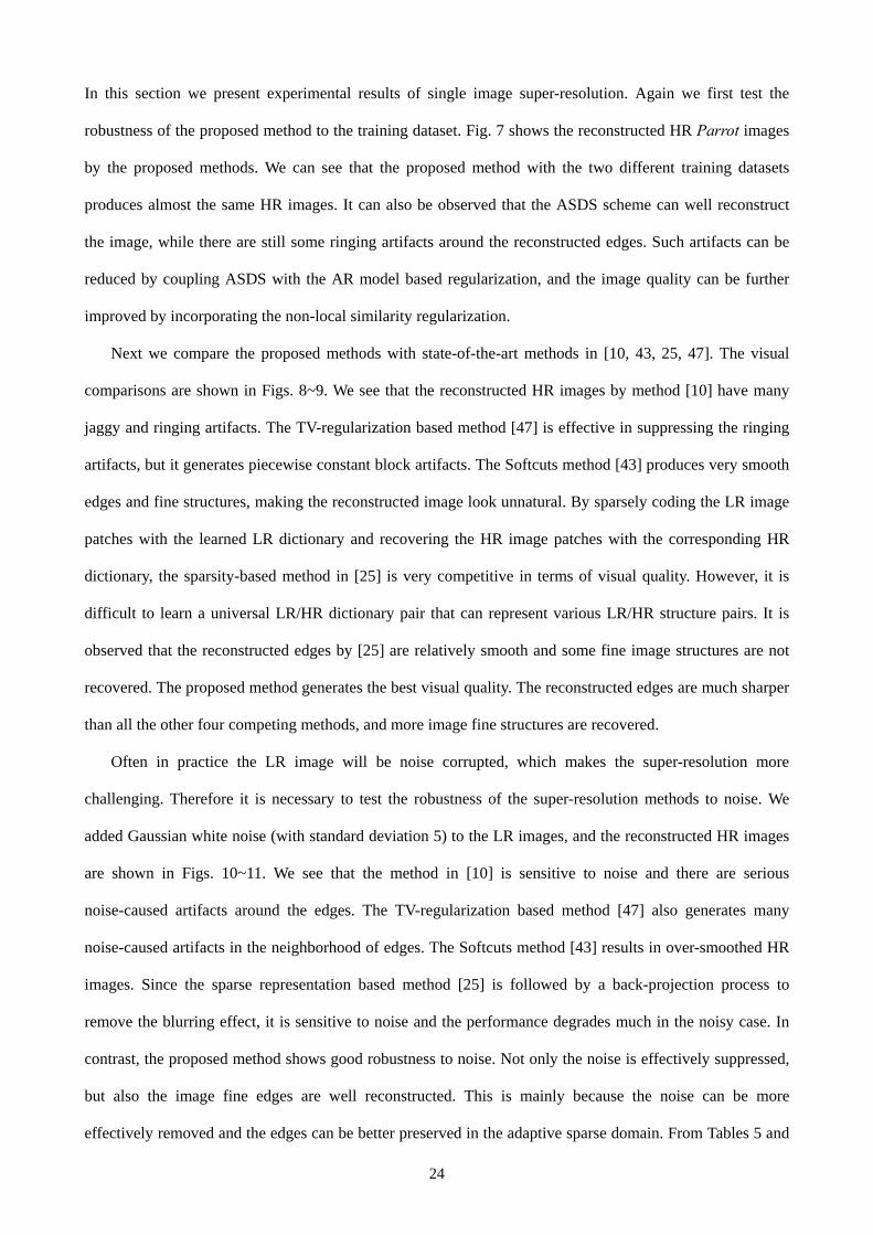
In this section we present experimental results of single image super-resolution. Again we first test the

robustness of the proposed method to the training dataset. Fig. 7 shows the reconstructed HR Parrot images

by the proposed methods. We can see that the proposed method with the two different training datasets

produces almost the same HR images. It can also be observed that the ASDS scheme can well reconstruct

the image, while there are still some ringing artifacts around the reconstructed edges. Such artifacts can be

reduced by coupling ASDS with the AR model based regularization, and the image quality can be further

improved by incorporating the non-local similarity regularization.

Next we compare the proposed methods with state-of-the-art methods in [10, 43, 25, 47]. The visual

comparisons are shown in Figs. 8~9. We see that the reconstructed HR images by method [10] have many

jaggy and ringing artifacts. The TV-regularization based method [47] is effective in suppressing the ringing

artifacts, but it generates piecewise constant block artifacts. The Softcuts method [43] produces very smooth

edges and fine structures, making the reconstructed image look unnatural. By sparsely coding the LR image

patches with the learned LR dictionary and recovering the HR image patches with the corresponding HR

dictionary, the sparsity-based method in [25] is very competitive in terms of visual quality. However, it is

difficult to learn a universal LR/HR dictionary pair that can represent various LR/HR structure pairs. It is

observed that the reconstructed edges by [25] are relatively smooth and some fine image structures are not

recovered. The proposed method generates the best visual quality. The reconstructed edges are much sharper

than all the other four competing methods, and more image fine structures are recovered.

Often in practice the LR image will be noise corrupted, which makes the super-resolution more

challenging. Therefore it is necessary to test the robustness of the super-resolution methods to noise. We

added Gaussian white noise (with standard deviation 5) to the LR images, and the reconstructed HR images

are shown in Figs. 10~11. We see that the method in [10] is sensitive to noise and there are serious

noise-caused artifacts around the edges. The TV-regularization based method [47] also generates many

noise-caused artifacts in the neighborhood of edges. The Softcuts method [43] results in over-smoothed HR

images. Since the sparse representation based method [25] is followed by a back-projection process to

remove the blurring effect, it is sensitive to noise and the performance degrades much in the noisy case. In

contrast, the proposed method shows good robustness to noise. Not only the noise is effectively suppressed,

but also the image fine edges are well reconstructed. This is mainly because the noise can be more

effectively removed and the edges can be better preserved in the adaptive sparse domain. From Tables 5 and

25

6, we see that the average PSNR gains of ASDS-AR-NL-TD2 over the second best methods [10] (for the

noiseless case) and [43] (for the noisy case) are 1.13 dB and 0.77 dB, respectively. The average SSIM gains

over the methods [10] and [43] are 0.0348 and 0.021 for the noiseless and noisy cases, respectively.

E. Experimental results on a 1000-image dataset

Fig. 12. Some example images in the established 1000-image dataset.

To more comprehensively test the robustness of the proposed IR method, we performed extensive deblurring

and super-resolution experiments on a large dataset that contains 1000 natural images of various contents. To

establish this dataset, we randomly downloaded 822 high-quality natural images from the Flickr website

(http://www.flickr.com/), and selected 178 high-quality natural images from the Berkeley Segmentation

Database3. A 256×256 sub-image that is rich in edge and texture structures was cropped from each of these

1000 images to test our method. Fig. 12 shows some example images in this dataset.

For image deblurring, we compared the proposed method with the methods in [46] and [58], which

perform the 2nd and the 3rd best in our experiments in Section VI-D. The average PSNR and SSIM values of

the deblurred images by the test methods are shown in Table 7. To better illustrate the advantages of the

proposed method, we also drew the distributions of its PSNR gains over the two competing methods in Fig.

13. From Table 7 and Fig. 13, we can see that the proposed method constantly outperforms the competing

methods for the uniform blur kernel, and the average PSNR gain over the BM3D [58] is up to 0.85 dB

(when σn= 2 ). Although the performance gaps between different methods become much smaller for the

non-truncated Gaussian blur kernel, it can still be observed that the proposed method mostly outperforms 3 http://www.eecs.berkeley.edu/Research/Projects/CS/vision/grouping/segbench

26

BM3D [58] and [46], and the average PSNR gain over BM3D [58] is up to 0.19 dB (when σn=2). For image

super-resolution, we compared the proposed method with the two methods in [25] and [47]. The average

PSNR and SSIM values by the test methods are listed in Table 8, and the distributions of PSNR gain of our

method over [25] and [47] are shown in Fig. 14. From Table 8 and Fig. 14, we can see that the proposed

method performs constantly better than the competing methods.

(a) (b)

(c) (d)

Fig. 13. The PSNR gain distributions of deblurring experiments. (a) Uniform blur kernel with σn= 2 ; (b) Uniform blur kernel with σn=2; (c) Gaussian blur kernel with σn= 2 ; (d) Gaussian blur kernel with σn=2.

(a) (b)

Fig. 14. The PSNR gain distributions of super-resolution experiments. (a) Noise level σn=0; (b) Noise level σn=5.

27

Fig. 15. Visual comparison of the deblurred images by the proposed method with different patch sizes. From left to right: patch size of 3×3, patch size of 5×5, and patch size of 7×7.

With this large dataset, we tested the robustness of the proposed method to the number of classes in

learning the sub-dictionaries and AR models. Specifically, we trained the sub-dictionaries and AR models

with different numbers of classes, i.e., 100, 200 and 400, and applied them to the established 1000-image

dataset. Table 9 presents the average PSNR and SSIM values of the restored images. We can see that the

three different numbers of classes lead to very similar image deblurring and super-resolution performance.

This illustrates the robustness of the proposed method to the number of classes.

Another important issue of the proposed method is the size of image patch. Clearly, the patch size

cannot be big; otherwise, they will not be micro-structures and hence cannot be represented by a small

number of atoms. To evaluate the effects of the patch size on IR results, we trained the sub-dictionaries and

AR models with different patch sizes, i.e., 3×3, 5×5 and 7×7. Then we applied these sub-dictionaries and AR

models to the 10 test images and the constructed 1000-image database. The experimental results of

deblurring and super-resolution are presented in Tables 10~12, from which we can see that these different

patch sizes lead to similar PSNR and SSIM results. However, it can be found that the smaller patch sizes (i.e.,

3×3 and 5×5) tend to generate some artifacts in smooth regions, as shown in Fig. 15. Therefore, we adopt

7×7 as the image patch size in our implementation.

F. Discussions on the computational cost

In Algorithm 1, the matrices U and V are sparse matrices, and can be pre-calculated after the initialization

of the AR models and the non-local weights. Hence, Step 2(a) can be executed fast. For image deblurring,

the calculation of ( )ˆ kUx can be implemented by FFT, which is faster than direct matrix calculation. Steps

2(b) and 2(d) require 2Nn multiplications, where n is the number of pixels of each patch and N is the

28

number of patches. In our implementation, N=NI /4, where NI is the number of pixels of the entire image.

Since each patch can be sparsely coded individually, Steps 2(b) and 2(d) can be executed in parallel to speed

up the algorithm. The update of sub-dictionaries and AR models requires N operations of nearest neighbor

search. We update them in every P iterations (P=100 in our implementation) to speed up Algorithm 1. As an

iterative shrinkage algorithm, the proposed Algorithm 1 converges in 700~1000 iterations in most cases.

For a 256×256 image, the proposed algorithm requires about 2~5 minutes for image deblurring and

super-resolution on an Intel Core2 Duo 2.79G PC under the Matlab R2010a programming environment. In

addition, several accelerating techniques, such as [51, 52], can be used to accelerate the convergence of the

proposed algorithm. Hence, the computational cost of the proposed method can be further reduced.

VII. Conclusion

We proposed a novel sparse representation based image deblurring and (single image) super-resolution

method using adaptive sparse domain selection (ASDS) and adaptive regularization (AReg). Considering the

fact that the optimal sparse domains of natural images can vary significantly across different images and

different image patches in a single image, we selected adaptively the dictionaries that were pre-learned from

a dataset of high quality example patches for each local patch. The ASDS improves significantly the

effectiveness of sparse modeling and consequently the results of image restoration. To further improve the

quality of reconstructed images, we introduced two AReg terms into the ASDS based image restoration

framework. A set of autoregressive (AR) models were learned from the training dataset and were used to

regularize the image local smoothness. The image non-local similarity was incorporated as another

regularization term to exploit the image non-local redundancies. An iterated shrinkage algorithm was

proposed to implement the proposed ASDS algorithm with AReg. The experimental results on natural

images showed that the proposed ASDS-AReg approach outperforms many state-of-the-art methods in both

PSNR and visual quality.

References

[1] M. Bertero and P. Boccacci, Introduction to Inverse Problems in Imaging. Bristol, U.K.: IOP, 1998. [2] D. Donoho, “Compressed sensing,” IEEE Trans. on Information Theory, vol. 52, no. 4, pp. 1289-1306,

April 2006.

29

[3] E. Candès and T. Tao, “Near optimal signal recovery from random projections: Universal encoding strategies?” IEEE Trans. on Information Theory, vol. 52, no. 12, pp. 5406 - 5425, December 2006.

[4] E. Candès, J. Romberg, and T. Tao, “Robust uncertainty principles: Exact signal reconstruction from highly incomplete frequency information,” IEEE Trans. on Information Theory, vol. 52, no. 2, pp. 489 - 509, February 2006.

[5] M. R. Banham and A. K. Katsaggelos, “Digital image restoration,” IEEE Trans. Signal Processing Mag., vol. 14, no. 2, pp. 24-41, Mar. 1997.

[6] L. Rudin, S. Osher, and E. Fatemi, “Nonlinear total variation based noise removal algorithms,” Phys. D, vol. 60, pp. 259–268, 1992.

[7] T. Chan, S. Esedoglu, F. Park, and A. Yip, “Recent developments in total variation image restoration,” in Mathematical Models of Computer Vision, N. Paragios, Y. Chen, and O. Faugeras, Eds. New York: Springer Verlag, 2005.

[8] S. Kindermann, S. Osher, and P. W. Jones, “Deblurring and denoising of images by nonlocal functionals,” Multiscale Modeling and Simulation, vol. 4, no. 4, pp. 1091-1115, 2005.

[9] R. Molina, J. Mateos, and A. K. Katsaggelos, “Blind deconvolution using a variational approach to parameter, image, and blur estimation,” IEEE Trans. On Image Process., vol. 15, no. 12, pp 3715-3727, Dec. 2006.

[10] I. Daubechies, M. Defriese, and C. DeMol, “An iterative thresholding algorithm for linear inverse problems with a sparsity constraint,” Commun. Pure Appl. Math., vol.57, pp.1413-1457, 2004.

[11] P. Combettes, and V. Wajs, “Signal recovery by proximal forward-backward splitting,” SIAM J.Multiscale Model.Simul., vol.4, pp.1168-1200, 2005.

[12] J.M. Bioucas Dias, and M.A.T. Figueiredo. “A new TwIST: two-step iterative shrinkage/thresholding algorithms for image restoration,” IEEE Trans. Image Proc., vol.16, no.12, pp.2992-3004, 2007.

[13] M. Elad, M.A.T. Figueiredo, and Y. Ma, “On the Role of Sparse and Redundant Representations in Image Processing,” Proceedings of IEEE, Special Issue on Applications of Compressive Sensing & Sparse Representation, June 2010.

[14] J. Mairal, M. Elad, and G. Sapiro, “Sparse Representation for Color Image Restoration,” IEEE Trans. on Image Processing, vol. 17, no. 1, pages 53-69, Jan. 2008.

[15] J. Mairal, F. Bach, J. Ponce, G. Sapiro and A. Zisserman, “Non-Local Sparse Models for Image Restoration,” International Conference on Computer Vision, Tokyo, Japan, 2009.

[16] M. Irani and S. Peleg, “Motion Analysis for Image Enhancement: Resolution, Occlusion, and Transparency,” Journal of Visual Communication and Image Representation, vol. 4, no. 4, pp. 324-335, Dec. 1993.

[17] S. D. Babacan, R. Molina, and A. K. Katsaggelos, “Total variation super resolution using a variational approach,” in Proc. Int. Conf. Image Proc, pp. 641-644, Oct. 2008.

[18] J. Oliveira, J. M. Bioucas-Dia, M. Figueiredo, and, “Adaptive total variation image deblurring: a majorization-minimization approach,” Signal Processing, vol. 89, no. 9, pp. 1683-1693, Sep. 2009.

[19] M. Lysaker and X. Tai, “Iterative image restoration combining total variation minimization and a second-order functional,” International Journal of Computer Vision, vol. 66, no. 1, pp. 5-18, 2006.

[20] X. Zhang, M. Burger, X. Bresson, and S. Osher, “Bregmanized nonlocal regularization for deconvolution and sparse reconstruction,” 2009. UCLA CAM Report (09-03).

[21] D. L. Donoho, “De-noising by soft thresholding,” IEEE Trans. Information Theory, vol. 41, pp. 613-627, May 1995.

[22] M. Elad and M. Aharon, “Image denoising via sparse and redundant representations over learned dictionaries,” IEEE Trans. Image Process., vol. 15, no. 12, pp. 3736-3745, Dec. 2006.

[23] M. J. Fadili and J. L. Starck, “Sparse representation-based image deconvolution by iterative thresholding,” Astronomical Data Analysis, Marseille, France, Sep. 2006.

[24] J. Bobin, J. Starck, J. Fadili, Y. Moudden, and D. Donoho, “Morphological Component Analysis: An Adaptive Thresholding Strategy”, IEEE Trans. Image processing, vol. 16, no. 11, pp. 2675-2681, 2007.

[25] J. Yang, J. Wright, Y. Ma, and T. Huang, “Image super-resolution as sparse representation of raw image patches,” IEEE Computer Vision and Pattern Recognition, Jun. 2008.

[26] M. Aharon, M. Elad, and A. Bruckstein, “K-SVD: an algorithm for designing overcomplete dictionaries for sparse representation,” IEEE Trans. Signal Process., vol. 54, no. 11, pp. 4311-4322, Nov. 2006.

[27] J. Mairal, G. Sapiro, and M. Elad, “Learning Multiscale Sparse Representations for Image and Video Restoration,” SIAM Multiscale Modeling and Simulation, vol. 7, no. 1, pages 214-241, April 2008.

[28] R. Rubinstein, M. Zibulevsky, and M. Elad, “Double sparsity: Learning Sparse Dictionaries for Sparse Signal Approximation,” IEEE Trans. Signal Processing, vol. 58, no. 3, pp. 1553-1564, March 2010.

30

[29] J. Mairal, F. Bach, J. Ponce, G. Sapiro, and A. Zisserman, “Supervised dictionary learning,” Advances in Neural Information Processing Systems (NIPS’08), pp. 1033-1040.

[30] G. Monaci and P. Vanderqheynst, “Learning structured dictionaries for image representation,” in Proc. IEEE Int. conf. Image Process., pp. 2351-2354, Oct. 2004.

[31] R. Rubinstein, A.M. Bruckstein, and M. Elad, “Dictionaries for sparse representation modeling,” Proceedings of IEEE, Special Issue on Applications of Compressive Sensing & Sparse Representation, vol. 98, no. 6, pp. 1045-1057, June, 2010.

[32] B. K. Gunturk, A. U. Batur, Y. Altunbasak, M. H. Hayes III, and R. M. Mersereau, “Eigenface-based super-resolution for face recognition,” in Proc. Int. conf. Image Process., pp. 845-848, Oct. 2002.

[33] X. Wu, K. U. Barthel, and W. Zhang, “Piecewise 2D autoregression for predictive image coding,” in Proc. Int. Conf. Image Process., vol. 3, pp. 901-904, Oct. 1998.

[34] X. Li and M. T. Orchard, “New edge-directed interpolation,” IEEE Trans. Image Process., vol. 10, no. 10, pp. 1521-1527, Oct. 2001.

[35] X. Zhang and X. Wu, “Image interpolation by 2-D autoregressive modeling and soft-decision estimation,” IEEE Trans. Image Process., vol. 17, no. 6, pp. 887-896, Jun. 2008.

[36] A. Buades, B. Coll, and J. M. Morel, “A review of image denoising algorithms, with a new one,” Multisc. Model. Simulat., vol. 4, no. 2, pp. 490.530, 2005.

[37] K. Fukunaga, Introduction to Statistical Pattern Recognition, 2nd Edition, Academic Press, 1991. [38] L. Zhang, R. Lukac, X. Wu, and D. Zhang, “PCA-based spatially adaptive denoising of CFA images for

single-sensor digital cameras,” IEEE Trans. Image Process., vol. 18, no. 4, pp. 797-812, Apr. 2009. [39] L. Zhang, W. Dong, D. Zhang, and G. Shi, “Two-stage image denoising by principal component

analysis with local pixel grouping,” Pattern Recognition, vol. 43, pp. 1531-1549, Apr. 2010. [40] X. Wu, X. Zhang, and J. Wang, “Model-guided adaptive recovery of compressive sensing,” in Proc.

Data Compression Conference, pp. 123-132, 2009. [41] M. Protter, M. Elad, H. Takeda, and P. Milanfar, “Generalizing the nonlocal-means to super-resolution

reconstruction,” IEEE Trans. On Image Process., vol. 18, no. 1, pp. 36-51, Jan. 2009. [42] A. Beck and M. Teboulle, “Fast gradient-based algorithms for constrained total variation image

denoising and deblurring problems,” IEEE Trans. On Image Process., vol. 18, no. 11, pp. 2419-2434, Nov. 2009.

[43] S. Dai, M. Han, W. Xu, Y. Wu, Y. Gong, and A. K. Katsaggelos, “SoftCuts: a soft edge smoothness prior for color image super-resolution,” IEEE Trans. Image Process., vol. 18, no. 5, pp. 969-981, May 2009.

[44] Z. Wang, A. C. Bovik, H. R. Sheikh, and E. P. Simoncelli, “Image quality assessment: from error measurement to structural similarity,” IEEE Trans. Image Process., vol. 3, no. 4, pp. 600-612, Apr. 2004.

[45] G. Chantas, N. P. Galatsanos, R. Molina, A. K. Katsaggelos, “Variational Bayesian image restoration with a product of spatially weighted total variation image priors,” IEEE Trans. Image Process., vol. 19, no. 2, pp. 351-362, Feb. 2010.

[46] J. Portilla, “Image restoration through l0 analysis-based sparse optimization in tight frames,” in Proc. IEEE Int. conf. Image Process., pp. 3909-3912, Nov. 2009.

[47] A. Marquina, and S. J. Osher, “Image super-resolution by TV-regularization and Bregman iteration,” J. Sci. Comput., vol. 37, pp. 367-382, 2008.

[48] S. Mallat and Z. Zhang, “Matching pursuits with time-frequency dictionaries,” IEEE Trans. Signal Process., vol. 41, no. 12, pp. 3397-3415, Dec. 1993.

[49] S. Chen, D. Donoho, and M. Saunders, “Atomic decompositions by basis pursuit,” SIAM Review, vol. 43, pp. 129-159, 2001.

[50] W. T. Freeman, T. R. Jones, and E. C. Pasztor, “Example-based super-resolution,” IEEE Comput. Graph. Appli., pp. 56-65, 2002.

[51] G. Narkiss and M. Zibulevsky, “Sequential subspace optimization method for large-scale unconstrained optimization,” Technical Report CCIT No. 559, Technion, Israel Institute of Technology, Haifa, 2005.

[52] A. Beck and M. Teboulle, “A fast iterative shrinkage thresholding algorithm for linear inverse problems,” SIAM J. Imaging Sciences, vol. 2, no. 1:183202, 2009.

[53] M. Elad, I. Yavneh, “A plurality of sparse representation is better than the sparsest one alone,” IEEE Trans. Information Theory, vol. 55, no. 10, pp. 4701-4714, Oct. 2009.

[54] M. Protter, I. Yavneh, and M. Elad, “Closed-form MMSE estimation for signal denoising under sparse representation modeling over a unitary dictionary,” IEEE Trans. Signal Processing, vol. 58, no. 7, pp. 3471-3484, July, 2010.

31

[55] A. M. Bruckstein, D. L. Donoho, and M. Elad, “From sparse solutions of systems of equations to sparse modeling of signals and images,” SIAM Review, vol. 51, no. 1, pp. 34-81, Feb. 2009.

[56] K. Engan, S. Aase, and J. Husoy, “Multi-frame compression: theory and design,” Signal Processing, vol. 80, no. 10, pp. 2121-2140, Oct. 2000.

[57] E. J. Candes, “Compressive sampling,” in Proc. of the International Congress of Mathematicians, Madrid, Spain, Aug. 2006.

[58] K. Dabov, A. Foi, V. Katkovnik, and K. Egiazarian, “Image restoration by sparse 3D transform-domain collaborative filtering,” in Society of Photo-Optical Instrumentation Engineers (SPIE) Conference Series, vol. 6812, 2008.

[59] E. Candes, M. B. Wakin, and S. P. Boyd, “Enhancing sparsity by reweighted l1 minimization,” Journal of Fourier Analysis and Applications, vol. 14, pp. 877-905, Dec. 2008.

[60] J. A. Tropp and S. J. Wright, “Computational methods for sparse solution of linear inverse problems,” Proceedings of IEEE, Special Issue on Applications of Compressive Sensing & Sparse Representation, vol. 98, no. 6, pp. 948-958, June, 2010.

[61] D. Field, “What is the goal of sensory coding?” Neural Computation, vol. 6, pp. 559-601, 1994. [62] B. Olshausen and D. Field, “Emergence of simple-cell receptive field properties by learning a sparse

code for natural images,” Nature, vol. 381, pp. 607-609, 1996. [63] B. Olshausen and D. Field, “Sparse coding with an overcomplete basis set: a strategy employed by

V1?” Vision Research, vol. 37, pp. 3311-3325, 1997.

32

Table 1. PSNR (dB) and SSIM results of deblurred images (uniform blur kernel, noise level σn= 2 ).

Images [10] [42] [45] [46] [58] ASDS- TD1

ASDS- TD2

ASDS- AR-TD1

ASDS- AR-TD2

ASDS-AR-NL-TD1

ASDS-AR-NL-TD2

Barbara 25.83 0.7492

25.59 0.7373

26.11 0.7580

26.28 0.7671

27.90 0.8171

26.60 0.7764

26.65 0.7709

26.93 0.7932

26.99 0.7893

27.63 0.8166

27.70 0.8192

Bike 23.09 0.6959

24.24 0.7588

24.38 0.7564

24.15 0.7530

24.77 0.7740

25.29 0.8014

25.50 0.8082

25.21 0.7989

25.40 0.8052

25.32 0.8003

25.48 0.8069

Straw 20.96 0.4856

21.31 0.5415

21.65 0.5594

21.32 0.5322

22.67 0.6541

22.32 0.6594

22.38 0.6651

22.39 0.6563

22.45 0.6615

22.51 0.6459

22.56 0.6540

Boats 28.80 0.8274

28.94 0.8331

29.44 0.8459

29.81 0.8496

29.90 0.8528

28.85 0.8076

28.94 0.8039

29.40 0.8286

29.48 0.8272

30.73 0.8665

30.76 0.8670

Parrots 27.80 0.8652

28.80 0.8704

28.96 0.8722

29.04 0.8824

30.22 0.8906

30.71 0.8926

30.90 0.8941

30.64 0.8920

30.79 0.8933

30.76 0.8921

30.92 0.8939

Baboon 21.06 0.4811

21.16 0.5095

21.33 0.5192

21.21 0.5126

21.46 0.5315

21.43 0.5881

21.45 0.5863

21.56 0.5878

21.55 0.5853

21.62 0.5754

21.62 0.5765

Hat 29.75 0.8393

31.13 0.8624

30.88 0.8567

30.91 0.8591

30.85 0.8608

31.46 0.8702

31.67 0.8736

31.41 0.8692

31.58 0.8721

31.43 0.8689

31.65 0.8733

Penta- gon

24.69 0.6452

25.12 0.6835

25.57 0.7020

25.26 0.6830

26.00 0.7210

25.58 0.7285

25.62 0.7290

25.88 0.7385

25.89 0.7380

26.41 0.7511

26.46 0.7539

Camera -man

25.73 0.8161

26.72 0.8330

27.38 0.8443

26.86 0.8361

27.24 0.8308

27.01 0.7956

27.14 0.7836

27.25 0.8255

27.37 0.8202

27.87 0.8578

28.00 0.8605

Peppers 27.89 0.8123

28.44 0.8131

28.87 0.8298

28.75 0.8274

28.70 0.8151

28.24 0.7749

28.25 0.7682

28.64 0.7992

28.68 0.7941

29.46 0.8357

29.51 0.8359

Average 25.56 0.7217

26.15 0.7443

26.46 0.7544

26.36 0.7500

26.97 0.7748

26.75 0.7695

26.85 0.7683

26.93 0.7789

27.02 0.7786

27.37 0.7910

27.47 0.7943

Table 2. PSNR (dB) and SSIM results of deblurred images (uniform blur kernel, noise level σn=2).

Images [10] [42] [45] [46] [58] ASDS- TD1

ASDS- TD2

ASDS- AR-TD1

ASDS- AR-TD2

ASDS-AR-NL-TD1

ASDS-AR-NL-TD2

Barbara 24.86 0.6963

25.12 0.7031

25.34 0.7214

25.37 0.7248

27.16 0.7881

26.33 0.7756

26.35 0.7695

26.45 0.7784

26.48 0.7757

26.89 0.7899

26.96 0.7927

Bike 22.30 0.6391

24.07 0.7487

23.61 0.7142

23.33 0.7049

24.13 0.7446

24.46 0.7608

24.61 0.7670

24.43 0.7599

24.58 0.7656

24.59 0.7649

24.72 0.7692

Straw 20.39 0.4112

21.07 0.5300

21.00 0.4885

20.81 0.4727

21.98 0.5946

21.78 0.5991

21.78 0.6027

21.79 0.5970

21.80 0.6008

21.81 0.5850

21.88 0.5934

Boats 27.47 0.7811

27.85 0.7880

28.66 0.8201

28.75 0.8181

29.19 0.8335

28.80 0.8145

28.83 0.8124

28.97 0.8195

29.00 0.8187

29.83 0.8441

29.83 0.8435

Parrots 26.84 0.8432

28.58 0.8595

28.06 0.8573

27.98 0.8665

29.45 0.8806

29.77 0.8787

29.98 0.8802

29.73 0.8784

29.94 0.8798

29.94 0.8800

30.06 0.8807

Baboon 20.58 0.4048

20.98 0.4965

20.87 0.4528

20.80 0.4498

21.13 0.4932

21.10 0.5441

21.10 0.5429

21.17 0.5428

21.16 0.5410

21.24 0.5285

21.24 0.5326

Hat 28.92 0.8153

30.79 0.8524

30.28 0.8433

30.15 0.8420

30.36 0.8507

30.71 0.8522

30.89 0.8556

30.69 0.8516

30.86 0.8550

30.80 0.8545

30.99 0.8574

Penta- gon

23.88 0.5776

24.59 0.6587

24.86 0.6516

24.54 0.6297

25.46 0.6885

25.34 0.7051

25.31 0.7042

25.42 0.7069

25.39 0.7066

25.74 0.7118

25.75 0.7146

Camera -man

24.80 0.7837

26.04 0.7772

26.53 0.8273

25.96 0.8131

26.53 0.8136

26.67 0.8211

26.81 0.8156

26.69 0.8243

26.86 0.8238

27.11 0.8365

27.25 0.8408

Peppers 27.04 0.7889

27.46 0.7660

28.33 0.8144

28.05 0.8106

28.15 0.7999

28.30 0.7995

28.24 0.7904

28.37 0.8038

28.37 0.7988

28.82 0.8204

28.87 0.8209

Average 24.71 0.6741

25.66 0.7180

25.75 0.7191

25.57 0.7132

26.35 0.7487

26.33 0.7551

26.39 0.7540

26.37 0.7562

26.44 0.7566

26.68 0.7615

26.75 0.7646

33

Table 3. PSNR (dB) and SSIM results of deblurred images (Gaussian blur kernel, noise level σn= 2 ).

Images [10] [42] [45] [46] [58] ASDS-TD1

ASDS-TD2

ASDS-AR-TD1

ASDS-AR-TD2

ASDS-AR-NL-TD1

ASDS-AR-NL-TD2

Barbara 23.65 0.6411

23.22 0.5971

23.19 0.5892

23.71 0.6460

23.77 0.6489

23.81 0.6560

23.81 0.6556

23.81 0.6566

23.81 0.6563

23.86 0.6609

23.86 0.6611

Bike 21.78 0.6085

21.90 0.6137

21.20 0.5515

22.20 0.6407

22.71 0.6774

22.59 0.6657

22.63 0.6693

22.59 0.6663

22.62 0.6688

22.80 0.6813

22.82 0.6830

Straw 20.28 0.4005

19.76 0.3502

19.33 0.2749

20.33 0.4087

21.02 0.5003

20.76 0.4710

20.81 0.4754

20.79 0.4729

20.82 0.4773

20.91 0.4866

20.93 0.4894

Boats 26.19 0.7308

25.53 0.7056

24.77 0.6688

26.64 0.7464

26.99 0.7486

27.12 0.7617

27.14 0.7633

27.11 0.7616

27.13 0.7625

27.27 0.7651

27.31 0.7677

Parrots 26.40 0.8321

25.96 0.8080

25.21 0.7949

26.84 0.8444

27.72 0.8580

27.42 0.8539

27.50 0.8538

27.45 0.8540

27.52 0.8540

27.67 0.8600

27.70 0.8598

Baboon 20.22 0.3622

20.01 0.3396

19.85 0.3011

20.24 0.3673

20.34 0.3923

20.36 0.3908

20.35 0.3889

20.36 0.3916

20.35 0.3893

20.39 0.3976

20.38 0.3959

Hat 28.11 0.7916

28.90 0.8100

28.29 0.7924

28.85 0.8122

28.87 0.8119

28.80 0.8074

28.92 0.8104

28.80 0.8074

28.89 0.8099

28.96 0.8110

29.01 0.8134

Penta- gon

23.33 0.5472

22.48 0.4881

22.09 0.4387

23.39 0.5540

23.82 0.5994

23.89 0.5974

23.88 0.5958

23.89 0.5978

23.89 0.5971

24.00 0.6086

24.01 0.6089

Camera -man

23.08 0.7332

23.26 0.7483

22.59 0.7187

23.51 0.7521

23.77 0.7249

23.85 0.7603

23.90 0.7637

23.83 0.7599

23.89 0.7630

24.03 0.7619

24.05 0.7649

Peppers 25.96 0.7666

25.58 0.7411

24.94 0.7236

26.61 0.7843

26.65 0.7626

26.99 0.7883

27.01 0.7900

26.98 0.7880

26.99 0.7898

27.12 0.7880

27.14 0.7902

Average 23.90 0.6414

23.66 0.6202

23.15 0.5854

24.23 0.6556

24.57 0.6724

24.56 0.6752

24.59 0.6766

24.56 0.6756

24.59 0.6768

24.70 0.6821

24.72 0.6834

Table 4. PSNR (dB) and SSIM results of deblurred images (Gaussian blur kernel, noise level σn=2).

Images [10] [42] [45] [46] [58] ASDS- TD1

ASDS- TD2

ASDS- AR-TD1

ASDS- AR-TD2

ASDS-AR-NL-TD1

ASDS-AR-NL-TD2

Barbara 23.57 0.6309

23.19 0.5933

23.07 0.5776

23.62 0.6351

23.70 0.6399

23.72 0.6464

23.72 0.6464

23.73 0.6468

23.73 0.6471

23.78 0.6520

23.78 0.6521

Bike 21.58 0.5903

21.88 0.6125

20.97 0.5324

21.93 0.6178

22.53 0.6643

22.41 0.6506

22.45 0.6527

22.41 0.6513

22.45 0.6536

22.66 0.6685

22.69 0.6704

Straw 20.10 0.3750

19.75 0.3499

19.24 0.2590

20.10 0.3781

20.81 0.4762

20.57 0.4471

20.60 0.4500

20.58 0.4484

20.62 0.4529

20.72 0.4664

20.75 0.4698

Boats 25.87 0.7157

25.48 0.7032

24.63 0.6602

26.24 0.7292

26.71 0.7359

26.78 0.7464

26.82 0.7488

26.81 0.7478

26.81 0.7487

26.98 0.7503

26.96 0.7521

Parrots 26.10 0.8234

25.92 0.8053

25.05 0.7907

26.38 0.8337

27.40 0.8523

27.08 0.8443

27.14 0.8447

27.13 0.8452

27.24 0.8460

27.47 0.8536

27.50 0.8535

Baboon 20.16 0.3497

20.00 0.3389

19.79 0.2905

20.17 0.3533

20.28 0.3826

20.28 0.3775

20.28 0.3758

20.29 0.3775

20.28 0.3762

20.32 0.3858

20.31 0.3839

Hat 27.94 0.7857

28.86 0.8084

28.27 0.7913

28.59 0.8043

28.67 0.8049

28.59 0.8009

28.69 0.8036

28.59 0.8009

28.69 0.8036

28.80 0.8056

28.87 0.8080

Penta- gon

23.13 0.5267

22.46 0.4876

21.89 0.4200

23.13 0.5299

23.65 0.5843

23.69 0.5784

23.69 0.5770

23.69 0.5793

23.70 0.5783

23.80 0.5922

23.81 0.5917

Camera -man

22.93 0.7256

23.23 0.7465

22.36 0.7130

23.25 0.7412

23.60 0.7198

23.72 0.7533

23.76 0.7568

23.71 0.7528

23.76 0.7564

23.95 0.7557

23.95 0.7583

Peppers 25.72 0.7570

25.50 0.7373

24.38 0.7034

26.24 0.7723

26.44 0.7555

26.70 0.7770

26.76 0.7800

26.71 0.7773

26.76 0.7804

26.91 0.7774

26.93 0.7799

Average 23.71 0.6280

23.63 0.6183

22.96 0.5738

23.97 0.6395

24.38 0.6616

24.36 0.6622

24.39 0.6636

24.37 0.6627

24.40 0.6643

24.54 0.6707

24.56 0.6720

34

Table 5. The PSNR (dB) and SSIM results (luminance components) of reconstructed HR images (noise levelσn=0).

Images [10] [43] [25] [47] ASDS- TD1

ASDS- TD2

ASDS-AR-TD1

ASDS-AR-TD2

ASDS-AR-NL-TD1

ASDS-AR-NL-TD2

Girl 32.93 0.8102

31.94 0.7704

32.51 0.7912

31.21 0.7878

33.40 0.8213

33.41 0.8215

33.42 0.8218

33.41 0.8216

33.54 0.8242

33.53 0.8242

Parrot 28.78 0.8845

27.71 0.8682

27.98 0.8665

27.59 0.8856

29.47 0.9031

29.51 0.9034

29.61 0.9036

29.63 0.9038

29.97 0.9090

30.00 0.9093

Butterfly 25.16 0.8336

25.19 0.8623

23.73 0.7942

26.60 0.9036

26.24 0.8775

26.27 0.8779

26.24 0.8758

26.23 0.8753

27.09 0.8975

27.34 0.9047

Leaves 24.59 0.8310

24.34 0.8372

24.35 0.8170

24.58 0.8878

25.94 0.8847

25.97 0.8856

25.93 0.8835

25.95 0.8842

26.78 0.9050

26.80 0.9058

Parthenon 26.32 0.7135

25.87 0.6791

24.08 0.6305

25.89 0.7163

26.63 0.7279

26.61 0.7278

26.63 0.7279

26.62 0.7277

26.82 0.7348

26.83 0.7349

Flower 28.16 0.8120

27.50 0.7800

27.76 0.7929

27.38 0.8111

28.80 0.8351

28.82 0.8354

28.82 0.8352

28.84 0.8358

29.19 0.8480

29.19 0.8480

Hat 29.92 0.8438

29.68 0.8389

29.65 0.8362

29.19 0.8569

30.70 0.8653

30.69 0.8648

30.65 0.8643

30.64 0.8641

30.92 0.8707

30.93 0.8706

Raccoon 28.80 0.7549

27.96 0.6904

28.49 0.7273

27.53 0.7076

29.06 0.7648

29.10 0.7658

29.11 0.7657

29.13 0.7664

29.23 0.7675

29.24 0.7677

Bike 23.48 0.7438

23.31 0.7219

23.20 0.7188

23.61 0.7567

24.10 0.7760

24.11 0.7772

24.08 0.7752

24.07 0.7752

24.48 0.7948

24.62 0.7962

Plants 31.87 0.8792

31.45 0.8617

31.48 0.8698

31.28 0.8784

32.85 0.8985

32.91 0.8996

32.85 0.8987

32.88 0.8995

33.47 0.9094

33.47 0.9095

Average 28.03 0.8115

27.49 0.7910

27.69 0.7954

27.49 0.8190

28.72 0.8354

28.74 0.8359

28.73 0.8352

28.74 0.8354

29.15 0.8461

29.16 0.8463

Table 6. The PSNR (dB) and SSIM results (luminance components) of reconstructed HR images (noise level σn=5).

Images [10] [43] [25] [47] ASDS- TD1

ASDS- TD2

ASDS-AR-TD1

ASDS-AR-TD2

ASDS-AR-NL-TD1

ASDS-AR-NL-TD2

Noisy Girl 30.37 0.7044

31.40 0.7480

30.70 0.7088

29.77 0.7258

31.72 0.7583

31.76 0.7596

31.72 0.7584

31.75 0.7594

31.79 0.7593

31.80 0.7590

Noisy Parrot

27.01 0.7911

27.42 0.8458

26.82 0.7769

26.77 0.8084

28.81 0.8673

28.91 0.8689

28.74 0.8634

28.83 0.8676

28.66 0.8632

28.72 0.8668

Noisy Butterfly

23.67 0.7777

24.95 0.8427

23.50 0.7576

25.47 0.8502

25.54 0.8362

25.76 0.8435

25.50 0.8350

25.61 0.8388

25.99 0.8591

26.08 0.8612

Noisy Leaves

23.62 0.7751

23.17 0.7939

23.35 0.7467

23.78 0.8457

25.14 0.8457

25.21 0.8491

25.11 0.8444

25.13 0.8455

25.49 0.8633

25.50 0.8645

Noisy Parthenon

25.31 0.6163

25.65 0.6587

23.89 0.5847

25.24 0.6651

26.06 0.6826

26.09 0.6845

26.06 0.6816

26.08 0.6826

26.09 0.6807

26.10 0.6821

Noisy Flower

26.61 0.6991

27.16 0.7591

26.51 0.7020

26.45 0.7509

27.58 0.7683

27.55 0.7699

27.64 0.7710

27.65 0.7733

27.67 0.7738

27.69 0.7767

Noisy Hat 28.14 0.6944

29.27 0.8049

28.32 0.7282

28.11 0.7768

29.56 0.8086

29.70 0.8151

29.50 0.8075

29.58 0.8129

29.57 0.8127

29.63 0.8175

Noisy Raccoon

27.05 0.6434

27.60 0.6707

27.20 0.6418

26.73 0.6640

27.98 0.6886

28.01 0.6882

27.99 0.6880

28.01 0.6876

28.01 0.6840

28.01 0.6810

Noisy Bike 22.74 0.6672

23.06 0.6984

22.42 0.6459

23.07 0.7118

23.49 0.7201

23.57 0.7239

23.43 0.7182

23.49 0.7205

23.52 0.7205

23.57 0.7220

Noisy Plants

29.93 0.7760

30.80 0.8343

29.51 0.7691

29.67 0.8028

31.01 0.8324

31.03 0.8342

30.95 0.8308

30.99 0.8327

31.09 0.8350

31.10 0.8363

Average 26.49 0.7048

27.05 0.7657

26.34 0.7090

26.52 0.7604

27.69 0.7808

27.76 0.7837

27.66 0.7798

27.71 0.7821

27.79 0.7851

27.82 0.7867

35

Table 7. Average PSNR and SSIM values of the deblurred images on the 1000-image dataset.

Method Uniform blur kernel

σn= 2 Uniform blur kernel

σn=2 Gaussian blur kernel

σn= 2 Gaussian blur kernel

σn=2

ASDS-AR-NL-TD2 29.36 (0.8397) 28.66 (0.8163) 26.22 (0.7335) 26.10 (0.7261) [58] 28.51 (0.8139) 27.96 (0.7966) 26.09 (0.7297) 25.91 (0.7209) [46] 28.26 (0.8081) 27.41 (0.7763) 25.63 (0.7072) 25.37 (0.6934)

Table 8. Average PSNR and SSIM results of the reconstructed HR images on the 1000-image dataset.

Method Noise level σn=0 Noise level σn=5

ASDS-AR-NL-TD2 27.53 (0.7975) 26.56 (0.7444)

[25] 26.26 (0.7444) 25.34 (0.6711)

[47] 26.09 (0.7705) 25.31 (0.7156) Table 9. Average PSNR and SSIM results by the proposed ASDS-AR-NL-TD2 method with different numbers of classes on the 1000-image dataset.

Number of classes Deblurring with uniform blur

kernel and σn= 2 Super-resolution with noise level

σn=0

100 29.29 (0.8379) 27.51 (0.7971)

200 29.36 (0.8397) 27.52 (0.7974) 400 29.31 (0.8380) 27.53 (0.7975)

Table 10. The PSNR and SSIM results of deblurred images by the proposed ASDS-AR-NL-TD2 with different patch sizes (uniform blurring kernel, σn= 2 ).

Patch Size Barbara Bike Straw Boats Parrots Baboon Hat Penta-

gon Camer-aman Peppers Average

3×3 27.33 0.7936

25.68 0.8173

22.32 0.6320

30.64 0.8651

31.07 0.9024

21.61 0.5713

32.12 0.8816

26.44 0.7509

28.09 0.8455

29.55 0.8270

27.49 0.7887

5×5 27.59 0.8116

25.54 0.8089

22.44 0.6428

30.81 0.8689

31.04 0.8968

21.61 0.5751

31.84 0.8745

26.48 0.7549

28.11 0.8599

29.63 0.8339

27.51 0.7927

7×7 27.70 0.8192

25.48 0.8069

22.56 0.6540

30.76 0.8670

30.92 0.8939

21.62 0.5765

31.65 0.8733

26.46 0.7553

28.00 0.8605

29.51 0.8359

27.47 0.7943

Table 11. The PSNR and SSIM results of reconstructed HR images by the proposed ASDS-AR-NL-TD2 with different patch sizes (noise level σn=0).

Patch Size Girl Parrot Butterfly Leaves Parthenon Flower Hat Raccoon Bike Plants Average

3×3 33.55 0.8251

29.96 0.9104

27.28 0.9055

27.00 0.9139

26.84 0.7366

29.27 0.8527

30.95 0.8739

29.18 0.7660

24.46 0.7961

33.54 0.9131

29.20 0.8493

5×5 33.56 0.8240

30.09 0.9121

27.39 0.9058

27.00 0.9118

26.90 0.7377

29.25 0.8500

31.10 0.8742

29.22 0.7664

24.53 0.7965

33.59 0.9116

29.26 0.8490

7×7 33.55 0.8204

30.14 0.9092

27.34 0.9047

26.93 0.9099

26.89 0.7357

29.19 0.8463

31.04 0.8716

29.24 0.7655

24.62 0.7962

33.37 0.9061

29.22 0.8464

Table 12. Average PSNR and SSIM results by the proposed ASDS-AR-NL-TD2 method with different patch sizes on the 1000-image dataset.

Patch size Deblurring with uniform blur

kernel and σn= 2 Super-resolution with noise level

σn=0

3×3 29.60 (0.8466) 27.51 (0.7979) 5×5 29.56 (0.8450) 27.54 (0.7984)

7×7 29.36 (0.8397) 27.53 (0.7976)