The Annals of Applied Statistics2008, Vol. 2, No. 2, 435–471DOI: 10.1214/07-AOAS137© Institute of Mathematical Statistics, 2008

TREELETS—AN ADAPTIVE MULTI-SCALE BASIS FOR SPARSEUNORDERED DATA

BY ANN B. LEE,1 BOAZ NADLER2 AND LARRY WASSERMAN1

Carnegie Mellon University, Weizmann Institute of Scienceand Carnegie Mellon University

In many modern applications, including analysis of gene expression andtext documents, the data are noisy, high-dimensional, and unordered—withno particular meaning to the given order of the variables. Yet, successfullearning is often possible due to sparsity: the fact that the data are typi-cally redundant with underlying structures that can be represented by onlya few features. In this paper we present treelets—a novel construction ofmulti-scale bases that extends wavelets to nonsmooth signals. The methodis fully adaptive, as it returns a hierarchical tree and an orthonormal basiswhich both reflect the internal structure of the data. Treelets are especiallywell-suited as a dimensionality reduction and feature selection tool prior toregression and classification, in situations where sample sizes are small andthe data are sparse with unknown groupings of correlated or collinear vari-ables. The method is also simple to implement and analyze theoretically. Herewe describe a variety of situations where treelets perform better than principalcomponent analysis, as well as some common variable selection and clusteraveraging schemes. We illustrate treelets on a blocked covariance model andon several data sets (hyperspectral image data, DNA microarray data, and in-ternet advertisements) with highly complex dependencies between variables.

1. Introduction. For many modern data sets (e.g., DNA microarrays, finan-cial and consumer data, text documents and internet web pages), the collecteddata are high-dimensional, noisy, and unordered, with no particular meaning tothe given order of the variables. In this paper we introduce a new methodologyfor the analysis of such data. We describe the theoretical properties of the method,and illustrate the proposed algorithm on hyperspectral image data, internet adver-tisements, and DNA microarray data. These data sets contain structure in the formof complex groupings of correlated variables. For example, the internet data in-clude more than a thousand binary variables (various features of an image) and

Received May 2007; revised August 2007.Discussed in 10.1214/08-AOAS137A, 10.1214/08-AOAS137B, 10.1214/08-AOAS137C,

10.1214/08-AOAS137D, 10.1214/08-AOAS137E and 10.1214/08-AOAS137F; rejoinder at10.1214/08-AOAS137REJ.

1Supported in part by NSF Grants CCF-0625879 and DMS-0707059.2Supported by the Hana and Julius Rosen fund and by the William Z. and Eda Bess Novick Young

Scientist fund.Key words and phrases. Feature selection, dimensionality reduction, multi-resolution analysis,

local best basis, sparsity, principal component analysis, hierarchical clustering, small sample sizes.

435

436 A. B. LEE, B. NADLER AND L. WASSERMAN

a couple of thousand observations (an image in an internet page). Some of thevariables are exactly linearly related, while others are similar in more subtle ways.The DNA microarray data include the expression levels of several thousand genesbut less than 100 samples (patients). Many sets of genes exhibit similar expressionpatterns across samples. The task in both cases is here classification. The resultscan therefore easily be compared with those of other classification algorithms.There is, however, a deeper underlying question that motivated our work: Is therea simple general methodology that, by construction, captures intrinsic localizedstructures, and that as a consequence improves inference and prediction of noisy,high-dimensional data when sample sizes are small? The method should be pow-erful enough to describe complex structures on multiple scales for unordered data,yet be simple enough to understand and analyze theoretically. Below we give somemore background to this problem.

The key property that allows successful inference and prediction in high-dimensional settings is the notion of sparsity. Generally speaking, there are twomain notions of sparsity. The first is sparsity of various quantities related eitherto the learning problem at hand or to the representation of the data in the orig-inal given variables. Examples include a sparse regression or classification vec-tor [Tibshirani (1996)], and a sparse structure to the covariance or inverse covari-ance matrix of the given variables [Bickel and Levina (2008)]. The second notion issparsity of the data themselves. Here we are referring to a situation where the data,despite their apparent high dimensionality, are highly redundant with underlyingstructures that can be represented by only a few features. Examples include datawhere many variables are approximately collinear or highly related, and data thatlie on a nonlinear manifold [Belkin and Niyogi (2005), Coifman et al. (2005)].1

While the two notions of sparsity are different, they are clearly related. In fact,a low intrinsic dimensionality of the data typically implies, for example, sparseregression or classification vectors, as well as low-rank covariance matrices. How-ever, this relation may not be directly transparent, as the sparsity of these quantitiessometimes becomes evident only in a different basis representation of the data.

In either case, to take advantage of sparsity, one constrains the set of possibleparameters of the problem. For the first kind of sparsity, two key tools are graphi-cal models [Whittaker (2001)] that assume statistical dependence between specificvariables, and regularization methods that penalize nonsparse solutions [Hastie,Tibshirani and Friedman (2001)]. Examples of such regularization methods are thelasso [Tibshirani (1996)], regularized covariance estimation methods [Bickel andLevina (2008), Levina and Zhu (2007)] and variable selection in high-dimensionalgraphs [Meinshausen and Bühlmann (2006)]. For the second type of sparsity,where the goal is to find a new set of coordinates or features of the data, two stan-dard “variable transformation” methods are principal component analysis [Jolliffe

1A referee pointed out that another issue with sparsity is that very high-dimensional spaces havevery simple structure [Hall, Marron and Neeman (2005), Murtagh (2004), Ahn and Marron (2008)].

TREELETS 437

(2002)] and wavelets [Ogden (1997)]. Each of these two methods has its ownstrengths and weaknesses which we briefly discuss here.

PCA has gained much popularity due to its simplicity and the unique propertyof providing a sequence of best linear approximations in a least squares sense. Themethod has two main limitations. First, PCA computes a global representation,where each basis vector is a linear combination of all the original variables. Thismakes it difficult to interpret the results and detect internal localized structures inthe data. For example, in gene expression data, it may be difficult to detect smallsubsets of highly correlated genes. The second limitation is that PCA constructsan optimal linear representation of the noisy observations, but not necessarily ofthe (unknown) underlying noiseless data. When the number of variables p is muchlarger than the number of observations n, the true underlying principal factorsmay be masked by the noise, yielding an inconsistent estimator in the joint limitp,n → ∞,p/n → c [Johnstone and Lu (2008)]. Even for a finite sample size n,this property of PCA and other global methods (such as partial least squares andridge regression) can lead to large prediction errors in regression and classifica-tion [Buckheit and Donoho (1995), Nadler and Coifman (2005b)]. Equation (25)in our paper, for example, gives an estimate of the finite-n regression error for alinear mixture error-in-variables model.

In contrast to PCA, wavelet methods describe the data in terms of localizedbasis functions. The representations are multi-scale, and for smooth data, alsosparse [Donoho and Johnstone (1995)]. Wavelets are used in many nonparametricstatistics tasks, including regression and density estimation. In recent years waveletexpansions have also been combined with regularization methods to find regres-sion vectors which are sparse in an a priori known wavelet basis [Candès and Tao(2007), Donoho and Elad (2003)]. The main limitation of wavelets is the implicitassumption of smoothness of the (noiseless) data as a function of its variables. Inother words, standard wavelets are not suited for the analysis of unordered data.Thus, some work suggests first sorting the data, and then applying fixed waveletsto the reordered data [Murtagh, Starck and Berry (2000), Murtagh (2007)].

In this paper we propose an adaptive method for multi-scale representation andeigenanalysis of data where the variables can occur in any given order. We callthe construction treelets, as the method is inspired by both hierarchical clusteringtrees and wavelets. The motivation for the treelets is two-fold: One goal is to finda “natural” system of coordinates that reflects the underlying internal structure ofthe data and that is robust to noise. A second goal is to improve the performanceof conventional regression and classification techniques in the “large p, small n”regime by finding a reduced representation of the data prior to learning. We payspecial attention to sparsity in the form of groupings of similar variables. Suchlow-dimensional structure naturally occurs in many data sets; for example, in DNAmicroarray data where genes sharing the same pathway can exhibit highly corre-lated expression patterns, and in the measured spectra of a chemical compound thatis a linear mixture of certain simpler substances. Collinearity of variables is often

438 A. B. LEE, B. NADLER AND L. WASSERMAN

a problem for a range of existing dimensionality reduction techniques—includingleast squares, and variable selection methods that do not take variable groupingsinto account.

The implementation of the treelet transform is similar to to the classical Jacobimethod from numerical linear algebra [Golub and van Loan (1996)]. In our workwe construct a data-driven multi-scale basis by applying a series of Jacobi rotations(PCA in two dimensions) to pairs of correlated variables. The final computed basisfunctions are orthogonal and supported on nested clusters in a hierarchical tree.As in standard PCA, we explore the covariance structure of the data but—unlikePCA—the analysis is local and multi-scale. As shown in Section 3.2.2 the treelettransform also has faster convergence properties than PCA. It is therefore moresuitable as a feature extraction tool when sample sizes are small.

Other methods also relate to treelets. In recent years hierarchical cluster-ing methods have been widely used for identifying diseases and groups of co-expressed genes [Eisen et al. (1998), Tibshirani et al. (1999)]. Many researchersare also developing algorithms that combine gene selection and gene grouping;see, for example, Hastie et al. (2001), Dettling and Bühlmann (2004), Zou andHastie (2005) among others, and see Fraley and Raftery (2002) for a review ofmodel-based clustering.

The novelty and contribution of our approach is the simultaneous constructionof a data-driven multi-scale orthogonal basis and a hierarchical cluster tree. Theintroduction of a basis enables application of the well-developed machinery of or-thonormal expansions, wavelets, and wavelet packets for nonparametric smooth-ing, data compression, and analysis of general unordered data. As with any ortho-normal expansion, the expansion coefficients reflect the effective dimension of thedata, as well as the significance of each coordinate. In our case, we even go onestep further: The basis functions themselves contain information on the geometryof the data, while the corresponding expansion coefficients indicate their impor-tance; see examples in Sections 4 and 5.

The treelet algorithm has some similarities to the local Karhunen–Loève Basisfor smooth ordered data by Coifman and Saito (1996), where the basis functionsare data-driven but the tree structure is fixed. Our paper is also related to recentindependent work on the Haar wavelet transform of a dendrogram by Murtagh(2007). The latter paper also suggests basis functions on a data-driven cluster treebut uses fixed wavelets on a pre-computed dendrogram. The treelet algorithm of-fers the advantages of both approaches, as it incorporates adaptive basis functionsas well as a data-driven tree structure. As shown in this paper, this unifying prop-erty turns out to be of key importance for statistical inference and prediction: Theadaptive tree structure allows analysis of unordered data. The adaptive treelet func-tions lead to results that reflect the internal localized structure of the data, and thatare stable to noise. In particular, when the data contain subsets of co-varying vari-ables, the computed basis is sparse, with the dominant basis functions effectivelyserving as indicator functions of the hidden groups. For more complex structure, as

TREELETS 439

illustrated on real data sets, our method returns “softer,” continuous-valued loadingfunctions. In classification problems, the treelet functions with the most discrimi-nant power often compute differences between groups of variables.

The organization of the paper is as follows: In Section 2 we describe the treeletalgorithm. In Section 3 we examine its theoretical properties. The analysis includesthe general large-sample properties of treelets, as well as a specific covariancemodel with block structure. In Section 4 we discuss the performance of the treeletmethod on a linear mixture error-in-variable model and give a few illustrative ex-amples of its use in data representation and regression. Finally, in Section 5 weapply our method to classification of hyperspectral data, internet advertisements,and gene expression arrays.

A preliminary version of this paper was presented at AISTATS-07 [Lee andNadler (2007)].

2. The treelet transform. In many modern data sets the data are not onlyhigh-dimensional but also redundant with many variables related to each other.Hierarchical clustering algorithms [Jain, Murty and Flynn (1999), Xu and Wunsch(2005)] are often used for the organization and grouping of the variables of suchdata sets. These methods offer an easily interpretable description of the data struc-ture in terms of a dendrogram, and only require the user to specify a measure ofsimilarity between groups of observations or variables. So called agglomerative hi-erarchical methods start at the bottom of the tree and, at each level, merge the twogroups with highest inter-group similarity into one larger cluster. The novelty ofthe proposed treelet algorithm is in constructing not only clusters or groupings ofvariables, but also functions on the data. More specifically, we construct a multi-scale orthonormal basis on a hierarchical tree. As in standard multi-resolutionanalysis [Mallat (1998)], the treelet algorithm provides a set of “scaling functions”defined on nested subspaces V0 ⊃ V1 ⊃ · · · ⊃ VL, and a set of orthogonal “de-tail functions” defined on residual spaces {W�}L�=1, where V� ⊕ W� = V�−1. Thetreelet decomposition scheme represents a multi-resolution transform, but techni-cally speaking, not a wavelet transform. (In terms of the tiling of “time-frequency”space, the method is more similar to local cosine transforms, which divide thetime axis in intervals of varying sizes.) The details of the treelet algorithm are inSection 2.1.

In this paper we measure the similarity Mij between two variables si and sjwith the correlation coefficient

ρij = �ij√�ii�jj

,(1)

where �ij = E[(si − Esi)(sj − Esj )] is the usual covariance. Other information-theoretic or graph-theoretic similarity measures are also possible. For some ap-plications, one may want to use absolute values of correlation coefficients, or aweighted sum of covariances and correlations as in Mij = |ρij | + λ|�ij |, wherethe parameter λ is a nonnegative number.

440 A. B. LEE, B. NADLER AND L. WASSERMAN

2.1. The algorithm: Jacobi rotations on pairs of similar variables. The treeletalgorithm is inspired by the classical Jacobi method for computing eigenvalues ofa matrix [Golub and van Loan (1996)]. There are also some similarities with theGrand Tour [Asimov (1985)], a visualization tool for viewing multidimensionaldata through a sequence of orthogonal projections. The main difference from Ja-cobi’s method—and the reason why the treelet transform, in general, returns anorthonormal basis different from standard PCA—is that treelets are constructed ona hierarchical tree.

The idea is simple. At each level of the tree, we group together the most simi-lar variables and replace them by a coarse-grained “sum variable” and a residual“difference variable.” The new variables are computed by a local PCA (or Jacobirotation) in two dimensions. Unlike Jacobi’s original method, difference variablesare stored, and only sum variables are processed at higher levels of the tree. Hence,the multi-resolution analysis (MRA) interpretation. The details of the algorithm areas follows:

• At level � = 0 (the bottom of the tree), each observation or “signal” x is rep-resented by the original variables x(0) = [s0,1, . . . , s0,p]T , where s0,k = xk . As-sociate to these coordinates, the Dirac basis, B0 = [φ0,1, φ0,2, . . . , φ0,p], whereB0 is the p × p identity matrix. Compute the sample covariance and similaritymatrices �(0) and M(0). Initialize the set of “sum variables,” S = {1,2, . . . , p}.

• Repeat for � = 1, . . . ,L:

1. Find the two most similar sum variables according to the similarity ma-trix M(�−1). Let

(α,β) = arg maxi,j∈S

M(�−1)ij ,(2)

where i < j , and maximization is only over pairs of sum variables that be-long to the set S. As in standard wavelet analysis, difference variables (de-fined in step 3) are not processed.

2. Perform a local PCA on this pair. Find a Jacobi rotation matrix

J (α,β, θ�) =

⎡⎢⎢⎢⎢⎢⎢⎢⎢⎢⎢⎣

1 · · · 0 · · · 0 · · · 0...

. . ....

......

0 · · · c · · · −s · · · 0...

.... . .

......

0 · · · s · · · c · · · 0...

......

. . ....

0 · · · 0 · · · 0 · · · 1

⎤⎥⎥⎥⎥⎥⎥⎥⎥⎥⎥⎦

,(3)

where c = cos(θ�) and s = sin(θ�), that decorrelates xα and xβ ; more specif-

ically, find a rotation angle θ� such that |θ�| ≤ π/4 and �(�)αβ = �

(�)βα = 0,

where �(�) = JT �(�−1)J . This transformation corresponds to a change of

TREELETS 441

basis B� = B�−1J , and new coordinates x(�) = JT x(�−1). Update the simi-larity matrix M(�) accordingly.

3. Multi-resolution analysis. For ease of notation, assume that �(�)αα ≥ �

(�)ββ

after the Jacobi rotation, where the indices α and β correspond to the first andsecond principal components, respectively. Define the sum and differencevariables at level � as s� = x

(�)α and d� = x

(�)β . Similarly, define the scaling

and detail functions φ� and ψ� as columns α and β of the basis matrix B�.Remove the difference variable from the set of sum variables, S = S \ {β}.At level �, we have the orthonormal treelet decomposition

x =p−�∑i=1

s�,iφ�,i +�∑

i=1

diψi,(4)

where the new set of scaling vectors {φ�,i}p−�i=1 is the union of the vector

φ� and the scaling vectors {φ�−1,j }j =α,β from the previous level, and the

new coarse-grained sum variables {s�,i}p−�i=1 are the projections of the original

data onto these vectors. As in standard multi-resolution analysis, the firstsum is the coarse-grained representation of the signal, while the second sumcaptures the residuals at different scales.

The output of the algorithm can be summarized in terms of a hierarchicaltree with a height L ≤ p − 1 and an ordered set of rotations and pairs of in-dices, {(θ�, α�, β�)}L�=1. Figure 1 (left) shows an example of a treelet construc-tion for a “signal” of length p = 5, with the data representations x(�) at thedifferent levels of the tree shown on the right. The s-components (projectionsin the main principal directions) represent coarse-grained “sums.” We associate

FIG. 1. (Left) A toy example of a hierarchical tree for data of dimension p = 5. At � = 0, thesignal is represented by the original p variables. At each successive level � = 1,2, . . . , p − 1, thetwo most similar sum variables are combined and replaced by the sum and difference variables s�, d�

corresponding to the first and second local principal components. (Right) Signal representation x(�)

at different levels. The s- and d-coordinates represent projections along scaling and detail functionsin a multi-scale treelet decomposition. Each such representation is associated with an orthogonalbasis in R

p that captures the local eigenstructure of the data.

442 A. B. LEE, B. NADLER AND L. WASSERMAN

these variables to the nodes in the cluster tree. Similarly, the d-components (pro-jections in the orthogonal directions) represent “differences” between node rep-resentations at two consecutive levels in the tree. For example, in the figured1ψ1 = (s0,1φ0,1 + s0,2φ0,2) − s1φ1,1.

We now briefly consider the complexity of the treelet algorithm on a generaldata set with n observations and p variables. For a naive implementation with anexhaustive search for the optimal pair (α,β) in Equation 2, the overall complexityis m+O(Lp2) operations, where m = O(min(np2,pn2)) is the cost of computingthe sample covariance matrix by singular value decomposition, and L is the heightof the tree. However, by storing the similarity matrices �(0) and M(0) and keepingtrack of their local changes, the complexity can be further reduced to m + O(Lp).In other words, the computational cost is comparable to hierarchical clusteringalgorithms.

2.2. Selecting the height L of the tree and a “best K-basis.” The default choiceof the treelet transform is a maximum height tree with L = p − 1; see examplesin Sections 5.1 and 5.3. This choice leads to a fully parameter-free decomposi-tion of the data and is also faithful to the idea of a multi-resolution analysis. Formore complexity, one can alternatively also choose any of the orthonormal (ON)bases at levels � < p − 1 of the tree. The data are then represented by coarse-grained sum variables for a set of clusters in the tree, and difference variables thatdescribe the finer details. In principle, any of the standard techniques in hierar-chical clustering can be used in deciding when to stop “merging” clusters (e.g.,use a preset threshold value for the similarity measure, or use hypothesis test-ing for homogeneity of clusters, etc.). In this work we propose a rather differentmethod that is inspired by the best basis paradigm [Coifman and Wickerhauser(1992), Saito and Coifman (1995)] in wavelet signal processing. This approachdirectly addresses the question of how well one can capture information in thedata.

Consider IID data x1, . . . ,xn, where xi ∈ Rp is a p-dimensional random vector.

Denote the candidate ON bases by B0, . . . ,Bp−1, where B� is the basis at level � inthe tree. Suppose now that we are interested in finding the “best” K-dimensionaltreelet representation for data representation and compression, where the dimen-sion K < p has been determined in advance. It then makes sense to use a scor-ing criterion that measures the percentage of explained variance for the chosencoordinates. Thus, we propose the following greedy scoring and selection ap-proach:

For a given orthonormal basis B = (w1, . . . ,wp), assign a normalized energyscore E to each vector wi according to

E(wi) = E{|wi · x|2}E{‖x‖2} .(5)

TREELETS 443

The corresponding sample estimate is E(w) =∑n

j=1 |wi ·xj |2∑nj=1 ‖xj‖2 . Sort the vectors ac-

cording to decreasing energy, w(1), . . . ,w(p), and define the score �K of the basisB by summing the K largest terms, that is, let �K(B) ≡∑K

i=1 E(wi). The bestK-basis is the treelet basis with the highest score

BL = arg maxB� : 0≤�≤p−1

�K(B�).(6)

It is the basis that best compresses the data with only K components. In case ofdegeneracies, we choose the coordinate system with the smallest �. Furthermore,to estimate the score �K for a particular data set, we use cross-validation (CV);that is, the treelets are constructed using subsets of the original data set and thescore is computed on independent test sets to avoid overfitting. Both theoreticalcalculations (Section 3.2) and simulations (Section 4.1) indicate that an energy-based measure is useful for detecting natural groupings of variables in data. Manyalternative measures (e.g., Fisher’s discriminant score, classification error rates,entropy, and other sparsity measures) can also be used. For the classification prob-lem in Section 5.1, for example, we define a discriminant score that measures howwell a coordinate separates data from different classes.

3. Theory.

3.1. Large sample properties of the treelet transform. In this section we ex-amine the large sample properties of treelets. We introduce a more general defini-tion of consistency that takes into account the fact that the treelet operator (basedon correlation coefficients) is multi-valued, and study the method under the statedconditions. We also describe a bootstrap algorithm for quantifying the stability ofthe algorithm in practical applications. The details are as follows.

First some notation and definitions: Let T (�) = J T �J denote the covari-ance matrix after one step of the treelet algorithm when starting with covariancematrix �. Let T �(�) denote the covariance matrix after � steps of the treeletalgorithm. Thus, T � = T ◦ · · · ◦ T corresponds to T applied � times. Define‖A‖∞ = maxj,k |Ajk| and let

Tn(�, δn) = ⋃‖�−�‖∞≤δn

T (�).(7)

Define T 1n (�, δn) = Tn(�, δn), and

T �n (�, δn) = ⋃

�∈T �−1n

T (�), � ≥ 2.(8)

Let �n denote the sample covariance matrix. We make the following assump-tions:

444 A. B. LEE, B. NADLER AND L. WASSERMAN

(A1) Assume that x has finite variance and satisfies one of the following threeassumptions: (a) each xj is bounded or (b) x is multivariate normal or (c) thereexist M and s such that E(|xjxk|q) ≤ q!Mq−2s/2 for all q ≥ 2.(A2) The dimension pn satisfies pn ≤ nc for some c > 0.

THEOREM 1. Suppose that (A1) and (A2) hold. Let δn = K√

logn/n, whereK > 2c. Then, as n,pn → ∞,

P(T �(�n) ∈ T �

n (�, δn), � = 1, . . . , pn

)→ 1.(9)

Some discussion is in order. The result says that T �(�n) is not too far fromT �(�) for some � close to �. It would perhaps be more satisfying to have aresult that says that ‖T �(�) − T �(�)‖∞ converges to 0. This would be possibleif one used covariances to measure similarity, but not in the case of correlationcoefficients.

For example, it is easy to construct a covariance matrix � with the followingproperties:

1. ρ12 is the largest off-diagonal correlation,2. ρ34 is nearly equal to ρ12,3. the 2 × 2 submatrix of � corresponding to x1 and x2 is very different than the

2 × 2 submatrix of � corresponding to x3 and x4.

In this case there is a nontrivial probability that ρ34 > ρ12 due to sample fluctua-tions. Therefore T (�) performs a rotation on the first two coordinates, while T (�)

performs a rotation on the third and fourth coordinates. Since the two correspond-ing submatrices are quite different, the two rotations will be quite different. Hence,T (�) can be quite different from T (�). This does not pose any problem since in-ferring T (�) is not the goal. Under the stated conditions, we would consider bothT (�) and T (�) to be reasonable transformations. We examine the details andinclude the proof of Theorem 1 in Appendix A.1.

Because T (�1) and T (�2) can be quite different even when the matrices �1and �2 are close, it might be of interest to study the stability of T (�n). This canbe done using the bootstrap. Construct B bootstrap replications of the data andcorresponding sample covariance matrices �∗

n,1, . . . , �∗n,B . Let δn = J−1

n (1 − α),

where Jn is the empirical distribution function of {‖�∗n,b − �n‖∞, b = 1, . . . ,B}

and α is the confidence level. If F has finite fourth moments and p is fixed, then itfollows from Corollary 1 of Beran and Srivastava (1985) that

limn→∞PF (� ∈ Cn) = 1 − α,

where Cn = {� :‖� − �n‖∞ ≤ δn}. Let

An = {T (�) :� ∈ Cn}.It follows that P(T (�) ∈ An) → 1 −α. The set An can be approximated by apply-ing T to all �∗

n,b for which ‖�∗n,b − �n‖∞ < δn. In Section 4.1 (Figure 3) we use

the bootstrap method to estimate confidence sets for treelets.

TREELETS 445

3.2. Treelets on covariance matrices with block structures.

3.2.1. An exact analysis in the limit n → ∞. Many real life data sets, includ-ing gene arrays, consumer data sets, and word-documents, display covariance ma-trices with approximate block structures. The treelet transform is especially wellsuited for representing and analyzing such data—even for noisy data and smallsample sizes.

Here we show that treelets provide a sparse representation when covariancematrices have inherent block structures, and that the loading functions themselvescontain information about the inherent groupings. We consider an ideal situationwhere variables within the same group are collinear, and variables from differ-ent groups are weakly correlated. All calculations are exact and computed in thelimit of the sample size n → ∞. An analysis of convergence rates later appears inSection 3.2.2.

We begin by analyzing treelets on p random variables that are indistinguishablewith respect to their second-order statistics. We show that the treelet algorithmreturns scaling functions that are constant on groups of indistinguishable variables.In particular, the scaling function on the full set of variables in a block is a constantfunction. Effectively, this function serves as an indicator function of a (sometimeshidden) set of similar variables in data. These results, as well as the follow-up mainresults in Theorem 2 and Corollary 1, are due to the fully adaptive nature of thetreelet algorithm—a property that sets treelets apart from methods that use fixedwavelets on a dendrogram [Murtagh (2007)], or adaptive basis functions on fixedtrees [Coifman and Saito (1996)]; see Remark 2 for a concrete example.

LEMMA 1. Assume that x = (x1, x2, . . . , xp)T is a random vector with dis-tribution F , mean 0, and covariance matrix � = σ 2

1 1p×p , where 1p×p denotes ap × p matrix with all entries equal to 1. Then, at any level 1 ≤ � ≤ p − 1 of thetree, the treelet operator T � (defined in Section 3.1) returns (for the populationcovariance matrix �) an orthogonal decomposition

T �(�) =p−�∑i=1

s�,iφ�,i +�∑

i=1

diψi,(10)

with sum variables s�,i = 1√|A�,i |∑

j∈A�,ixj and scaling functions φ�,i = 1√|A�,i | ×

Is�,i , which are defined on disjoint index subsets A�,i ⊆ {1, . . . , p} (i = 1, . . . , p −�) with lengths |A�,i | and

∑p−�i=1 |A�,i | = p. The expansion coefficients have vari-

ances V{s�,i} = |A�,i |σ 21 , and V{di} = 0. In particular, for � = p − 1,

T p−1(�) = sφ +p−1∑i=1

diψi,(11)

where s = 1√p(x1 + · · · + xp) and φ = 1√

p[1 . . .1]T .

446 A. B. LEE, B. NADLER AND L. WASSERMAN

REMARK 1. Uncorrelated additive noise in (x1, x2, . . . , xp) adds a diagonalperturbation to the 2 × 2 covariance matrices �(�), which are computed at eachlevel in the tree [see (35)]. Such noise may affect the order in which variables aregrouped, but the asymptotic results of the lemma remain the same.

REMARK 2. The treelet algorithm is robust to noise because it computesdata-driven rotations on variables. On the other hand, methods that use fixedtransformations on pre-computed trees are often highly sensitive to noise, yield-ing inconsistent results. Consider, for example, a set of four statistically indis-tinguishable variables {x1, x2, x3, x4}, and compare treelets to a Haar wavelettransform on a data-driven dendrogram [Murtagh (2004)]. The two methods re-turn the same results if the variables are merged in the order {{x1, x2}, {x3, x4}};that is, s = 1

2(x1 + x2 + x3 + x4) and φ = 12 [1,1,1,1]T . Now, a different real-

ization of the noise may lead to the order {{{x1, x2}, x4}, x3}. A fixed rotationangle of π/4 (as in Haar wavelets) would then return the sum variable sHaar =

1√2( 1√

2( 1√

2(x1 +x2)+x4)+x3) and scaling function φHaar = [ 1

2√

2, 1

2√

2, 1√

2, 1

2 ]T .

Next we consider data where the covariance matrix is a K × K block matrixwith white noise added to the original variables. The following main result statesthat, if variables from different blocks are weakly correlated and the noise levelis relatively small, then the K maximum variance scaling functions are constanton each block (see Figure 2 in Section 4 for an example). We make this preciseby giving a sufficient condition [equation (13)] in terms of the noise level, andwithin-block and between-block correlations of the original data. For illustrativepurposes, we have reordered the variables. A p × p identity matrix is denoted byIp , and a pi × pj matrix with all entries equal to 1 is denoted by 1pi×pj

.

THEOREM 2. Assume that x = (x1, x2, . . . , xp)T is a random vector with dis-tribution F , mean 0 and covariance matrix � = C + σ 2Ip , where σ 2 representsthe variance of white noise in each variable and

C =

⎛⎜⎜⎜⎝

C11 C12 . . . C1K

C12 C22 . . . C2K...

.... . .

...

C1K C2K . . . CKK

⎞⎟⎟⎟⎠(12)

is a K ×K block matrix with “within-block” covariance matrices Ckk = σ 2k 1pk×pk

(k = 1, . . . ,K) and “between-block” covariance matrices Cij = σij 1pi×pj(i, j =

1, . . . ,K ; i = j ). If

max1≤i,j≤K

(σij

σiσj

)<

1√1 + 3 max(δ2, δ4)

,(13)

TREELETS 447

where δ = σmink σk

, then the treelet decomposition at level � = p − K has the form

T p−K(�) =K∑

k=1

skφk +p−K∑i=1

diψi,(14)

where sk = 1√pk

∑j∈Bk

xj , φk = 1√pk

IBk, and Bk represents the set of indices

of variables in block k (k = 1, . . . ,K). The expansion coefficients have meansE{sk} = E{di} = 0, and variances V{sk} = pkσ

2k + σ 2 and V{di} = O(σ 2), for

i = 1, . . . , p − K .

Note that if the conditions of the theorem are satisfied, then all treelets (bothscaling and difference functions) associated with levels � > p −K are constant ongroups of similar variables. In particular, for a full decomposition at the maximumlevel � = p −1 of the tree we have the following key result, which follows directlyfrom Theorem 2:

COROLLARY 1. Assume that the conditions in Theorem 2 are satisfied. A fulltreelet decomposition then gives T p−1(�) = sφ +∑p−1

i=1 diψi, where the scalingfunction φ and the K −1 detail functions ψp−K+1, . . . ,ψp−1 are constant on eachof the K blocks. The coefficients s and dp−K+1, . . . , dp−1 reflect between-blockstructures, as opposed to the coefficients d1, . . . , dp−K which only reflect noise inthe data with variances V{di} = O(σ 2) for i = 1, . . . , p − K .

The last result is interesting. It indicates a parameter-free way of finding K ,the number of blocks, namely, by studying the energy distribution of a full treeletdecomposition. Furthermore, the treelet transform can uncover the block structureeven if it is hidden amidst a large number of background noise variables (see Fig-ure 3 for a simulation with finite sample size).

REMARK 3. Both Theorem 2 and Corollary 1 can be directly generalized toinclude p0 uncorrelated noise variables, so that x = (x1, . . . , xp−p0, xp−p0+1, . . . ,

xp)T , where E(xi) = 0 and E(xixj ) = 0 for i > p − p0 and j = i. For example, ifequation (13) is satisfied, then the treelet decomposition at level � = p − p0 is

T p−p0(�) =K∑

k=1

skφk +p−p0−K∑

i=1

diψi + (0, . . . ,0, xp−p0+1, . . . , xp)T .

Furthermore, note that according to equation (41) in the Appendix A.3, within-block correlations are smallest (“worst-case scenario”) when singletons aremerged. Thus, the treelet transform is a stabilizing algorithm; once a few cor-rect coarse-grained variables have been computed, it has the effect of denoisingthe data.

448 A. B. LEE, B. NADLER AND L. WASSERMAN

3.2.2. Convergence rates. The aim of this section is to give a rough estimateof the sample size required for treelets to discover the inherent structures of data.For covariance matrices with block structures, we show that treelets find the correctgroupings of variables if the sample size n � O(logp), where p is the dimensionof the data. This is a significant result, as standard PCA—on the other hand—is consistent if and only if p/n → 0 [Johnstone and Lu (2008)], that is, whenn � O(p). The result is also comparable to that in Bickel and Levina (2008) forregularization of sparse nearly diagonal covariance matrices. One main differenceis that their paper assumes an a priori known ordered set of variables in which thecovariance matrix is sparse, whereas treelets find such an ordering and coordinatesystem as part of the algorithm. The argument for treelets and a block covariancemodel goes as follows.

Assume that there are K blocks in the population covariance matrix �. DefineAL,n as the event that the K maximum variance treelets, constructed at level L =p−K of the tree, for a data set with n observations, are supported only on variablesfrom the same block. In other words, let AL,n represent the ideal case where thetreelet transform finds the exact groupings of variables. Let E� denote the eventthat at level � of the tree, the largest between-block sample correlation is less thanthe smallest within-block sample correlation,

E� = {max ρ(�)B < min ρ

(�)W

}.

According to equations (31)–(32), the corresponding population correlations

maxρ(�)B < ρ1 ≡ max

1≤i,j≤K

(σij

σiσj

), minρ

(�)W > ρ2 ≡ 1√

1 + 3 max(δ2, δ4),

where δ = σmink σk

, for all �. Thus, a sufficient condition for E� is that {max |ρ(�)B −

ρ(�)B | < t} ∩ {max |ρ(�)

W − ρ(�)W | < t} , where t = (ρ2 − ρ1)/2 > 0. We have that

P(AL,n) ≥ P

( ⋂0≤�<L

E�

)

≥ P

( ⋂0≤�<L

{max

∣∣ρ(�)B − ρ

(�)B

∣∣< t}∩ {max

∣∣ρ(�)W − ρ

(�)W

∣∣< t})

.

If (A1) holds, then it follows from Lemma 3 that

P(ACL,n) ≤ ∑

0≤�<L

(P(max

∣∣ρ(�)B − ρ

(�)B

∣∣> t)+ P

(max

∣∣ρ(�)W − ρ

(�)W

∣∣> t))

≤ Lc1p2e−nc2t

2

for positive constants c1, c2. Thus, the requirement P(ACL,n) < α is satisfied if the

sample size

n ≥ 1

c2t2 log(

Lc1p2

α

).

TREELETS 449

From the large-sample properties of treelets (Section 3.1), it follows that treeletsare consistent if n � O(logp).

4. Treelets and a linear error-in-variables mixture model. In this sectionwe study a simple error-in-variables linear mixture model (factor model) which,under some conditions, gives rise to covariance matrices with block structures.Under this model, we compare treelets with PCA and variable selection methods.An advantage of introducing a concrete generative model is that we can easilyrelate our results to the underlying structures or components of real data; for ex-ample, different chemical substances in spectroscopy data, genes from the samepathway in microarray data, etc.

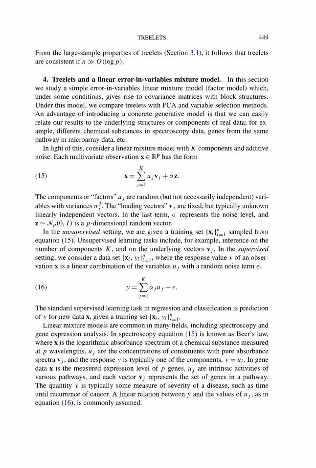
In light of this, consider a linear mixture model with K components and additivenoise. Each multivariate observation x ∈ R

p has the form

x =K∑

j=1

uj vj + σz.(15)

The components or “factors” uj are random (but not necessarily independent) vari-ables with variances σ 2

j . The “loading vectors” vj are fixed, but typically unknownlinearly independent vectors. In the last term, σ represents the noise level, andz ∼ Np(0, I ) is a p-dimensional random vector.

In the unsupervised setting, we are given a training set {xi}ni=1 sampled fromequation (15). Unsupervised learning tasks include, for example, inference on thenumber of components K , and on the underlying vectors vj . In the supervisedsetting, we consider a data set {xi , yi}ni=1, where the response value y of an obser-vation x is a linear combination of the variables uj with a random noise term ε,

y =K∑

j=1

αjuj + ε.(16)

The standard supervised learning task in regression and classification is predictionof y for new data x, given a training set {xi , yi}ni=1.

Linear mixture models are common in many fields, including spectroscopy andgene expression analysis. In spectroscopy equation (15) is known as Beer’s law,where x is the logarithmic absorbance spectrum of a chemical substance measuredat p wavelengths, uj are the concentrations of constituents with pure absorbancespectra vj , and the response y is typically one of the components, y = ui . In genedata x is the measured expression level of p genes, uj are intrinsic activities ofvarious pathways, and each vector vj represents the set of genes in a pathway.The quantity y is typically some measure of severity of a disease, such as timeuntil recurrence of cancer. A linear relation between y and the values of uj , as inequation (16), is commonly assumed.

450 A. B. LEE, B. NADLER AND L. WASSERMAN

4.1. Treelets and a linear mixture model in the unsupervised setting. Considerdata {xi}ni=1 from the model in equation (15). Here we analyze an illustrative ex-ample with K = 3 components and loading vectors vk = I (Bk), where I is the in-dicator function, and Bk ⊂ {1,2, . . . , p} are sets of variables with sizes pk = |Bk|(k = 1,2,3). A more general analysis is possible but may not provide more insight.

The unsupervised task is to uncover the internal structure of the linear mix-ture model from data, for example, to infer the unknown structure of the vec-tors vk , including the sizes pk of the sets Bk . The difficulty of this problem de-pends, among other things, on possible correlations between the random variablesuj , the variances of the components uj , and interferences (overlap) between theloading vectors vk . We present three examples with increasing difficulty. Standardmethods, such as principal component analysis, succeed only in the simplest case(Example 1), whereas more sophisticated methods, such as sparse PCA (elasticnets), sometimes require oracle information to correctly fit tuning parameters inthe model. The treelet transform seems to perform well in all three cases. More-over, the results are easy to explain by computing the covariance matrix of thedata.

EXAMPLE 1 (Uncorrelated factors and nonoverlapping loading vectors). Thesimplest case is when the random variables uj are all uncorrelated for j = 1,2,3,and the loading vectors vj are nonoverlapping. The population covariance matrixof x is then given by � = C + σ 2Ip , where the noise-free matrix

C =

⎛⎜⎜⎝

C11 0 0 00 C22 0 00 0 C33 00 0 0 0

⎞⎟⎟⎠(17)

is a 4 × 4 block matrix with the first three blocks Ckk = σ 2k 1pk×pk

(k = 1,2,3),and the last diagonal block having all entries equal to zero.

Assume that σk � σ for k = 1,2,3. This is a specific example of a spiked co-variance model [Johnstone (2001)] the three components corresponding to distinctlarge eigenvalues or “spikes” of a model with background noise. As n → ∞ withp fixed, PCA recovers the hidden vectors v1, v2, and v3, since these three vectorsexactly coincide with the principal eigenvectors of �. A treelet transform with aheight L determined by cross-validation and a normalized energy criterion returnsthe same results—which is consistent with Section 3.2 (Theorem 2 and Corol-lary 1).

The difference between PCA and treelets becomes obvious in the “small n,large p regime.” In the joint limit p,n → ∞, standard PCA computes consistentestimators of the vectors vj (in the presence of noise) if and only if p(n)/n →0 [Johnstone and Lu (2008)]. For an analysis of PCA for finite p,n, see, for exam-ple, Nadler (2007). As described in Section 3.2.2, treelets require asymptoticallyfar fewer observations with the condition for consistency being logp(n)/n → 0.

TREELETS 451

EXAMPLE 2 (Correlated factors and nonoverlapping loading vectors). If therandom variables uj are correlated, treelets are far better than PCA at inferring theunderlying localized structure of the data—even asymptotically. Again, this is easyto explain and quantify by studying the data covariance structure. For example,assume that the loading vectors v1, v2, and v3 are nonoverlapping, but that thecorresponding factors are dependent according to

u1 ∼ N(0, σ 21 ), u2 ∼ N(0, σ 2

2 ), u3 = c1u1 + c2u2.(18)

The covariance matrix is then given by � = C + σ 2Ip , where

C =

⎛⎜⎜⎝

C11 0 C13 00 C22 C23 0

C13 C23 C33 00 0 0 0

⎞⎟⎟⎠(19)

with Ckk = σ 2k 1pk×pk

(note that σ 23 = c2

1σ21 + c2

2σ22 ), C13 = c1σ

21 1p1×p3 , and

C23 = c2σ22 1p2×p3 . Due to the correlations between uj , the loading vectors of the

block model no longer coincide with the principal eigenvectors, and it is difficultto extract them with PCA.

We illustrate this problem by the example in Zou, Hastie and Tibshirani (2006).Specifically, let

v1 = [B1︷ ︸︸ ︷

1 1 1 1

B2︷ ︸︸ ︷0 0 0 0

B3︷︸︸︷0 0 ]T ,

v2 = [0 0 0 0 1 1 1 1 0 0 ]T ,(20)

v3 = [0 0 0 0 0 0 0 0 1 1 ]T ,

where there are p = 10 variables total, and the sets Bj are disjoint with p1 = p2 =4,p3 = 2 variables, respectively. Let σ 2

1 = 290, σ 22 = 300, c1 = −0.3, c2 = 0.925,

and σ = 1. The corresponding variance σ 23 of u3 is 282.8, and the covariances of

the off-diagonal blocks are σ13 = −87 and σ23 = 277.5.The first three PCA vectors for a training set of 1000 samples are shown in

Figure 2 (left). It is difficult to infer the underlying vectors vi from these results,as ideally, we would detect that, for example, the variables (x5, x6, x7, x8) are allrelated and extract the latent vector v2 from only these variables. Simply thresh-olding the loadings and discarding small values also fails to achieve this goal [Zou,Hastie and Tibshirani (2006)]. The example illustrates the limitations of a globalapproach even with an infinite number of observations. In Zou, Hastie and Tibshi-rani (2006) the authors show by simulation that a combined L1 and L2-penalizedleast squares method, which they call sparse PCA or elastic nets, correctly identi-fies the sets of important variables if given “oracle information” on the number ofvariables p1,p2,p3 in the different blocks. Treelets are similar in spirit to elasticnets as both methods tend to group highly correlated variables together. In this ex-ample the treelet algorithm is able to find both K , the number of components in

452 A. B. LEE, B. NADLER AND L. WASSERMAN

FIG. 2. In Example 2 PCA fails to find the important variables in the three-component mixturemodel, as the computed eigenvectors (left) are sensitive to correlations between different components.On the other hand, the three maximum energy treelets (right) uncover the underlying data structures.

the mixture model, and the hidden loading vectors vi—without any a priori knowl-edge or parameter tuning. Figure 2 (right) shows results from a treelet simulationwith a large sample size (n = 1000) and a height L = 7 of the tree, determined bycross-validation (CV) and an energy criterion. The three maximum energy basisvectors correspond exactly to the hidden loading vectors in equation (20).

EXAMPLE 3 (Uncorrelated factors and overlapping loading vectors). Finally,we study a challenging example where the first two loading vectors v1 and v2 areoverlapping, the sample size n is small, and the background noise level is high. Let{B1, . . . ,B4} be disjoint subsets of {1, . . . , p}, and let

v1 = I (B1) + I (B2), v2 = I (B2) + I (B3), v3 = I (B4),(21)

where I (Bk) as before represents the indicator function for subset k (k = 1, . . . ,4).The population covariance matrix is then given by � = C +σ 2Ip , where the noise-less matrix has the general form

C =

⎛⎜⎜⎜⎜⎝

C11 C12 0 0 0C12 C22 C23 0 00 C23 C33 0 00 0 0 C44 00 0 0 0 0

⎞⎟⎟⎟⎟⎠ ,(22)

with diagonal blocks C11 = σ 21 1p1×p1 , C22 = (σ 2

1 + σ 22 )1p2×p2 , C33 = σ 2

2 1p3×p3 ,C44 = σ 2

3 1p4×p4 , and off-diagonal blocks C12 = σ 21 1p1×p2 and C23 = σ 2

2 1p2×p3 .Consider a numerical example with n = 100 observations, p = 500 variables, andnoise level σ = 0.5. We choose the same form for the components u1, u2, u3 asin [Bair et al. (2006)], but associate the first two components with overlappingloading vectors v1 and v2. Specifically, the components are given by u1 = ±0.5

TREELETS 453

with equal probability, u2 = I (U2 < 0.4), and u3 = I (U3 < 0.3), where I (x)

is the indicator of x, and Uj are all independent uniform random variables in[0,1]. The corresponding variances are σ 2

1 = 0.25, σ 22 = 0.24, and σ 2

3 = 0.21.As for the blocks Bk , we consider B1 = {1, . . . ,10},B2 = {11, . . . ,50},B3 ={51, . . . ,100}, and B4 = {201, . . . ,400}.

Inference in this case is challenging for several different reasons. The sam-ple size n < p, the loading vectors v1 and v2 are overlapping in the regionB2 = {11, . . . ,50}, and the signal-to-noise ratio is low with the variance σ 2 of thenoise essentially being of the same size as the variances σ 2

j of uj . Furthermore, thecondition in equation (13) is not satisfied even for the population covariance ma-trix. Despite these difficulties, the treelet algorithm is remarkably stable, returningresults that by and large correctly identify the internal structures of the data. Thedetails are summarized below.

Figure 3 (top center) shows the energy score of the best K-basis at differentlevels of the tree. We used 5-fold cross-validation; that is, we generated a singledata set of n = 100 observations, but in each of the 5 computations the treeletswere constructed on a subset of 80 observations, with 20 observations left outfor the energy score computation. The five curves as well as their average clearly

FIG. 3. Top left: The vectors v1 (blue), v2 (green), v3 (red) in Example 3. Top center: The “score”or total energy of K = 3 maximum variance treelets computed at different levels of the tree with5-fold cross-validation; dotted lines represent the five different simulations and the solid line theaverage score. Top right: Energy distribution of the treelet basis for the full data set at an “optimal”height L = 300. Bottom left: The four treelets with highest energy. Bottom right: 95% confidencebands by bootstrap for the two dominant treelets.

454 A. B. LEE, B. NADLER AND L. WASSERMAN

indicate a “knee” at the level L = 300. This is consistent with our expectationsthat the treelet algorithm mainly merges noise variables at levels L ≥ |⋃k Bk|.For a tree with “optimum” height L = 300, as indicated by the CV results, wethen constructed a treelet basis on the full data set. Figure 3 (top right) shows theenergy of these treelets sorted according to descending energy score. The resultsindicate that we have two dominant treelets, while the remaining treelets have anenergy that is either slightly higher or of the same order as the variance of thenoise. In Figure 3 (bottom left) we plot the loadings of the four highest energytreelets. “Treelet 1” (red) is approximately constant on the set B4 (the support ofv3), “Treelet 2” (blue) is approximately piecewise constant on blocks B1, B2, andB3 (the support of v1 and v2), while the low-energy degenerate treelets 3 (green)and 4 (magenta) seem to take differences between variables in the sets B1, B2,and B3. Finally, we computed 95% confidence bands of the treelets using 1000bootstrap samples and the method described in Section 3.1. Figure 3 (bottom right)indicate, that the treelet results for the two maximum energy treelets are ratherstable despite the small sample size and the low signal-to-noise ratio. Most of thetime the first treelet selects variables from B4, and most of the time the secondtreelet selects variables from B2 and either B1 or B3 or both sets. The low-energytreelets seem to pick up differences between blocks B1, B2, and B3, but the exactorder in which they select the variables vary from simulation to simulation. Asdescribed in the next section, for the purpose of regression, the main point is thatthe linear span of the first few highest energy treelets is a good approximation ofthe span of the unknown loading vectors, Span{v1, . . . ,vK}.

4.2. The treelet transform as a feature selection scheme prior to regression.Knowing some of the basic properties of treelets, we now examine a typical re-gression or classification problem with data {xi , yi}ni=1 given by equations (15)and (16). As the data x are noisy, this is an error-in-variables type problem. Givena training set, the goal is to construct a linear function f : Rp → R to predicty = f (x) = r · x + b for a new observation x.

Before considering the performance of treelets and other algorithms in this set-ting, we review some of the properties of the optimal mean-squared error (MSE)predictor. For simplicity, we consider the case y = u1 in equation (16), and denoteby P1 : Rp → R

p the projection operator onto the space spanned by the vectors{v2, . . . ,vK}. In this setting the unbiased MSE-optimal estimator has a regressionvector r = vy/‖vy‖2, where vy = v1 − P1v1. The vector vy is the part of the load-ing vector v1 that is unique to the response variable y = u1, since the projection ofv1 onto the span of the loading vectors of the other components (u2, . . . , uK ) hasbeen subtracted. For example, in the case of only two components, we have that

vy = v1 − v1 · v2

‖v2‖2 v2.(23)

TREELETS 455

The vector vy plays a central role in chemometrics, where it is known as the netanalyte signal [Lorber, Faber and Kowalski (1997), Nadler and Coifman (2005a)].Using this vector for regression yields a mean squared error of prediction

E{(y − y)2} = σ 2

‖vy‖2 .(24)

We remark that, similar to shrinkage in point estimation, there exist biased esti-mators with smaller MSE [Gruber (1998), Nadler and Coifman (2005b)], but forlarge signal to noise ratios (σ/‖vy‖ � 1), such shrinkage is negligible.

Many regression methods [including multivariate least squares, partial leastsquares (PLS), principal component regression (PCR), etc.] attempt to computethe optimal regression vector or net analyte signal (NAS). It can be shown that inthe limit n → ∞, both PLS and PCR are MSE-optimal. However, in some appli-cations, the number of variables is much larger than the number of observations(p � n). The question at hand is then, what the effect of small sample size ison these methods, when combined with noisy high-dimensional data. Both PLSand PCR first perform a global dimensionality reduction from p to k variables,and then apply least squares linear regression on these k features. As described inNadler and Coifman (2005b), their main limitation is that in the presence of noisyhigh dimensional data, the computed projections are noisy themselves. For fixedp and n, a Taylor expansion of the regression coefficient as a function of the noiselevel σ shows that these methods have an averaged prediction error

E{(y − y)2} � σ 2

‖vy‖2

[1 + c1

n+ c2 σ 2

μ‖vy‖2

p2

n2

(1 + o(1)

)].(25)

In equation (25) the coefficients c1 and c2 are both O(1) constants, independent ofσ , p, and n. The quantity μ depends on the specific algorithm used, and is a mea-sure of the variances and covariances of the different components uj , and of theamount of interferences of their loading vectors vj . The key point of this analysisis that when p � n, the last term in (25) can dominate and lead to large predictionerrors. This emphasizes the limitations of global dimensionality reduction meth-ods, and the need for robust feature selection and dimensionality reduction of thedata prior to application of learning algorithms such as PCR and PLS.

Other common approaches to dimensionality reduction in this setting are vari-able selection schemes, specifically those that choose a small subset of variablesbased on their individual correlation with the response y. To analyze their per-formance, we consider a more general dimensionality reduction transformationT : Rp → R

k defined by k orthonormal projections wi ∈ Rp ,

T x = (x · w1,x · w2, . . . ,x · wk).(26)

This family of transformations includes variable subset selection methods, whereeach projection wj selects one of the original variables. It also includes wavelet

456 A. B. LEE, B. NADLER AND L. WASSERMAN

methods and our proposed treelet transform. Since an orthonormal projection ofa Gaussian noise vector in R

p is a Gaussian vector in Rk , and a relation similar

to equation (15) holds between T x and y, formula (25) still holds, but with theoriginal dimension p replaced by k, and with vy replaced by its projection T vy ,

E{(y − y)2} � σ 2

‖T vy‖2

[1 + c1

n+ c2 σ 2

μ‖T vy‖2

k2

n2

(1 + o(1)

)].(27)

Equation (27) indicates that a dimensionality reduction scheme should ideally pre-serve the net analyte signal of y (‖T vy‖ � ‖vy‖), while at the same time representthe data by as few features as possible (k � p).

The main problem of PCA is that it optimally fits the noisy data, yielding for thenoise-free response ‖T vy‖/‖vy‖ � (1 − cσ 2p2/n2). The main limitation of vari-able subset selection schemes is that in complex settings with overlapping vectorsvj , such schemes may at best yield ‖T vy‖/‖vy‖ < 1. Due to high dimension-ality, the latter methods may still achieve better prediction errors than methodsthat use all the original variables. However, with a more general variable transfor-mation/compression method, one could potentially better capture the NAS. If thedata x are a priori known to be smooth continuous signals, a reasonable choice iswavelet compression, which is known to be asymptotically optimal. In the case ofunstructured data, we propose to use treelets.

To illustrate these points, we revisit Example 3 in Section 4.1, and comparetreelets to the variable subset selection scheme of Bair et al. (2006) for PLS, as wellas global PLS on all variables. As before, we consider a relatively small trainingset of size n = 100 but here we include 1500 additional noise variables, so thatp = 2000 � n. We furthermore assume that the response is given by y = 2u1. Thevectors vj are shown in Figure 3 (top left). The two vectors v1 and v2 overlap, butv1 (associated with the response) and v3 are orthogonal. Therefore, the responsevector unique to y (the net analyte signal) is given by equation (23); see Figure 4(left).

To compute vy , all the 100 first coordinates (the set B1 ∪ B2 ∪ B3) are needed.However, a feature selection scheme that chooses variables based on their cor-relation to the response will pick the first 10 coordinates and then the next 40,that is, only variables in the set B1 ∪ B2 (the support of the loading vector v1).Variables numbered 51 to 100 (set B3), although critical for prediction of the re-sponse y = 2u1, are uncorrelated with it (as u1 and u2 are uncorrelated) and arethus not chosen, even in the limit n → ∞. In contrast, even in the presence ofmoderate noise and a relatively small sample size of n = 100, the treelet algorithmcorrectly joins together the subsets of variables 1–10, 11–50, 51–100 and 201–400(i.e., variables in the sets B1,B2,B3,B4). The rest of the variables, which con-tain only noise, are combined only at much higher levels in the treelet algorithm,as they are asymptotically uncorrelated. Because of this, using only coarse-grained

TREELETS 457

FIG. 4. Left: The vector vy (only the first 150 coordinates are shown as the rest are zero). Right:Averaged prediction errors of 20 simulation results for the methods, from top to bottom: PLS on allvariables (blue), supervised PLS with variable selection (purple), PLS on treelet features (green),and PLS on projections onto the true vectors vi (red).

sum variables in the treelet transform yields near optimal prediction errors. In Fig-ure 4 (right) we plot the mean squared error of prediction (MSEP) for 20 differ-ent simulations with prediction error computed on an independent test set of 500observations. The different methods are PLS on all variables (MSEP = 0.17), su-pervised PLS with variable selection as in Bair et al. (2006) (MSEP = 0.09), PLSon the 50 treelet features with highest variance, with the level of the treelet deter-mined by leave-one-out cross validation (MSEP = 0.035), and finally PLS on theprojection of the noisy data onto the true vectors vi , assuming they were known(MSEP = 0.030). In all cases, the optimal number of PLS projections (latent vari-ables) is also determined by leave-one-out cross validation. Due to the high dimen-sionality of the data, choosing a subset of the original variables performs betterthan full-variable methods. However, choosing a subset of treelet features per-forms even better, yielding an almost optimal prediction error (σ 2/‖vy‖2 ≈ 0.03);compare the green and red curves in the figure.

5. Examples.

5.1. Hyperspectral analysis and classification of biomedical tissue. To illus-trate how our method works for data with highly complex dependencies betweenvariables, we use an example from hyperspectral imaging of biomedical tissue.Here we analyze a hyperspectral image of an H&E stained microarray section ofnormal human colon tissue [see Angeletti et al. (2005) for details on the data col-lection method]. This is an ordered data set of moderate to high dimension. Onescan of the tissue specimen returns a 1024 × 1280 data cube or “hyperspectral im-age,” where each pixel location contains spectral measurements at 28 known fre-quencies between 420 nm and 690 nm. These spectra give information about the

458 A. B. LEE, B. NADLER AND L. WASSERMAN

chemical structure of the tissue. There is, however, redundancy as well as noise inthe spectra. The challenge is to find the right coordinate system for this relativelyhigh-dimensional space, and extract coordinates (features) that contain the mostuseful information about the chemicals and substances of interest.

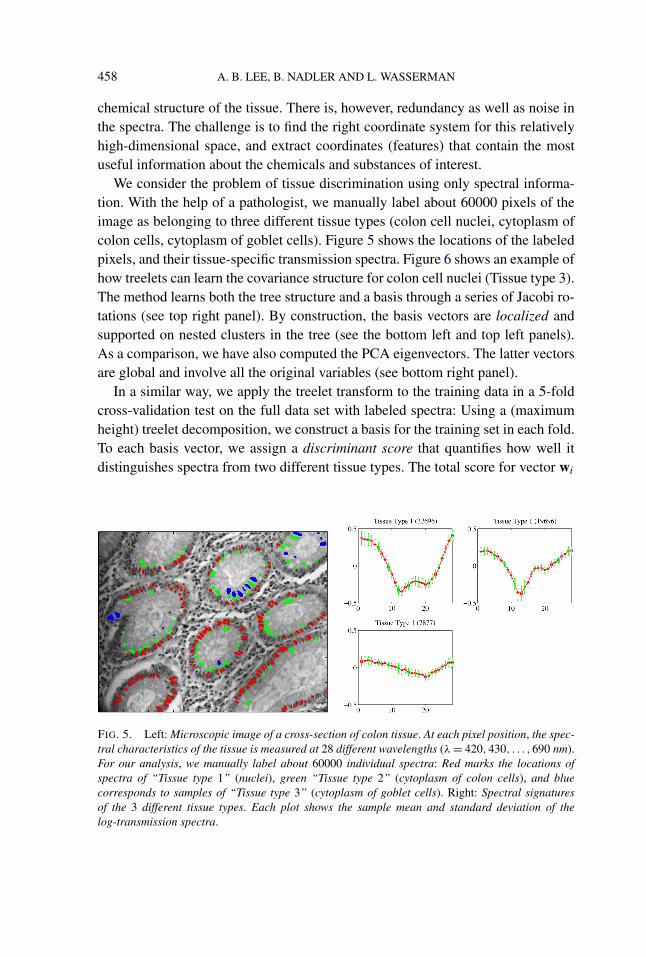
We consider the problem of tissue discrimination using only spectral informa-tion. With the help of a pathologist, we manually label about 60000 pixels of theimage as belonging to three different tissue types (colon cell nuclei, cytoplasm ofcolon cells, cytoplasm of goblet cells). Figure 5 shows the locations of the labeledpixels, and their tissue-specific transmission spectra. Figure 6 shows an example ofhow treelets can learn the covariance structure for colon cell nuclei (Tissue type 3).The method learns both the tree structure and a basis through a series of Jacobi ro-tations (see top right panel). By construction, the basis vectors are localized andsupported on nested clusters in the tree (see the bottom left and top left panels).As a comparison, we have also computed the PCA eigenvectors. The latter vectorsare global and involve all the original variables (see bottom right panel).

In a similar way, we apply the treelet transform to the training data in a 5-foldcross-validation test on the full data set with labeled spectra: Using a (maximumheight) treelet decomposition, we construct a basis for the training set in each fold.To each basis vector, we assign a discriminant score that quantifies how well itdistinguishes spectra from two different tissue types. The total score for vector wi

FIG. 5. Left: Microscopic image of a cross-section of colon tissue. At each pixel position, the spec-tral characteristics of the tissue is measured at 28 different wavelengths (λ = 420,430, . . . ,690 nm).For our analysis, we manually label about 60000 individual spectra: Red marks the locations ofspectra of “Tissue type 1” (nuclei), green “Tissue type 2” (cytoplasm of colon cells), and bluecorresponds to samples of “Tissue type 3” (cytoplasm of goblet cells). Right: Spectral signaturesof the 3 different tissue types. Each plot shows the sample mean and standard deviation of thelog-transmission spectra.

TREELETS 459

FIG. 6. Top left: Learned tree structure for nuclei (Tissue Type 1). In the dendrogram the height ofeach U-shaped line represents the distance dij = (1−ρij )/2, where ρij is the correlation coefficientfor the two variables combined. The leaf nodes represent the p = 28 original spectral bands. Topright: 2D scatter plots of the data at levels � = 1, . . . , p − 1. Each plot shows 500 randomly chosendata points; the lines indicate the first principal directions and rotations relative to the variables thatare combined. (Note that a Haar wavelet corresponds to a fixed π/4 rotation.) Bottom left: Learnedorthonormal basis. Each row represents a localized vector, supported on a cluster in the hierarchicaltree. Bottom right: Basis computed by a global eigenvector analysis (PCA).

is defined as

E(wi ) =K∑

j=1

K∑k=1;k =j

H(p

(j)i ||p(k)

i

),(28)

where K = 3 is the number of classes, and H(p(j)i ||p(k)

i ) is the Kullback–Leibler

distance between the estimated marginal density functions p(j)i and p

(k)i of class-j

and class-k signals, respectively, in the direction of wi . We project our trainingdata onto the K (< 28) most discriminant directions, and build a Gaussian classi-fier in this reduced feature space. This classifier is finally used to label the test dataand to estimate the misclassification error rate. The left panel in Figure 7 shows the

460 A. B. LEE, B. NADLER AND L. WASSERMAN

FIG. 7. Left: Average misclassification rate (in a 5-fold cross-validation test) as a function of thenumber of top discriminant features retained, for a treelet decomposition (rings), and for Haar-Walshwavelet packets (crosses). The constant level around 2.5% indicates the performance of a classifierdirectly applied to the 28 components in the original coordinate system. Right: The top 3 localdiscriminant basis (LDB) vectors in a treelet decomposition of the full data set.

average CV error rate as a function of the number of local discriminant features.(As a comparison, we show similar results for Haar–Walsh wavelet packets anda local discriminant basis [Saito, Coifman, Geshwind and Warner (2002)] whichuse the same discriminant score to search through a library of orthonormal waveletbases.) The straight line represents the error rate if we apply a Gaussian classifierdirectly to the 28 components in the original coordinate system. The key point isthat, with 3 treelet features, we get the same performance as if we used all the orig-inal data. Using more treelet features yields an even lower misclassification rate.(Because of the large sample size, the curse of dimensionality is not noticeablefor < 15 features.) These results indicate that a treelet representation has advan-tages beyond the obvious benefits of a dimensionality reduction. We are effectively“denoising” the data by changing our coordinate system and discarding irrelevantcoordinates. The right panel in Figure 7 shows the three most discriminant treeletvectors for the full data set. These vectors resemble continuous-valued versionsof the indicator functions in Section 3.2. Projecting onto one of these vectors hasthe effect of first taking a weighted average of adjacent spectral bands, and thencomputing a difference between averages of bands in different regions of the spec-trum. (In Section 5.3, Figure 10, we will see another example that the loadingsthemselves contain information about structure in data.)

5.2. A classification example with an internet advertisement data set. Here westudy an internet advertisement data set from the UCI ML repository [Kushmerick(1999)]. This is an example of an unordered data set of high dimension wheremany variables are collinear. After removal of the first three continuous variables,this set contains 1555 binary variables and 3279 observations, labeled as belonging

TREELETS 461

TABLE 1Classification test errors for an internet advertisement data set

Classifier Full data set Reduced data set Final representation with(1555 variables) (760 variables) coarse-grained treelet features

LDA 5.5% 5.1% 4.5%1-NN 4.0% 4.0% 3.7%

to one of two classes. The goal is to predict whether a new observation (an imagein an internet page) is an internet advertisement or not, given values of its 1555variables (various features of the image).

With standard classification algorithms, one can easily obtain a generalizationerror of about 5%. The first column in Table 1, labeled “full data set,” shows themisclassification rate for linear discriminant analysis (LDA) (with the additionalassumption of a diagonal covariance matrix), and for 1-nearest neighbor (1-NN)classification. The average is taken over 25 randomly selected training and testsets, with 3100 and 179 observations each.

The internet-ad data set has several distinctive properties that are clearly re-vealed by an analysis with treelets: First of all, several of the original variablesare exactly linearly related. As the data are binary (−1 or 1), these variables areeither identical or of opposite values. In fact, one can reduce the dimensionality ofthe data from 1555 to 760 without loss of information. The second column in thetable labeled “reduced data set” shows the decrease in error rate after a losslesscompression where we have simply removed redundant variables. Furthermore,of these remaining 760 variables, many are highly related, with subsets of sim-ilar variables. The treelet algorithm automatically identifies these groups, as thealgorithm reorders the variables during the basis computation, encoding the infor-mation in such a group with a coarse-grained sum variable and difference variablesfor the residuals. Figure 8, left, shows the correlation matrix of the first 200 out of760 variables in the order they are given. To the right, we see the correspondingmatrix, after sorting all variables according to the order in which they are com-bined by the treelet algorithm. Note how the (previously hidden) block structures“pop out.”

A more detailed analysis of the reduced data set with 760 variables shows thatthere are more than 200 distinct pairs of variables with a correlation coefficientlarger than 0.95. Not surprisingly, as shown in the right column of Table 1, treeletscan further increase the predictive performance on this data set, yielding resultscompetitive with other feature selection methods in the literature [Zhao and Liu(2007)]. All results in Table 1 are averaged over 25 different simulations. As inSection 4.2, the results are achieved at a level L < p − 1, by projecting the dataonto the treelet scaling functions, that is, by only using coarse-grained sum vari-ables. The height L of the tree is found by 10-fold cross-validation and a minimumprediction error criterion.

462 A. B. LEE, B. NADLER AND L. WASSERMAN

FIG. 8. Left: The correlation matrix of the first 200 out of 760 variables in the order they wereoriginally given. Right: The corresponding matrix, after sorting all variables according to the orderin which they are combined by the treelet algorithm.

5.3. Classification and analysis of DNA microarray data. We conclude withan application to DNA microarray data. In the analysis of gene expression, manymethods first identify groups of highly correlated variables and then choose afew representative genes for each group (a so-called gene signature). The treeletmethod also identifies subsets of genes that exhibit similar expression patterns, butin contrast, replaces each such localized group by a linear combination that en-codes the information from all variables in that group. As illustrated in previousexamples in the paper, such a representation typically regularizes the data whichimproves the performance of regression and classification algorithms.

Another advantage is that the treelet method yields a multi-scale data repre-sentation well-suited for the application. The benefits of hierarchical clustering inexploring and visualizing microarray data are well recognized in the field [Eisenet al. (1998), Tibshirani et al. (1999)]. It is, for example, known that a hierarchicalclustering (or dendrogram) of genes can sometimes reveal interesting clusters ofgenes worth further investigation. Similarly, a dendrogram of samples may identifycases with similar medical conditions. The treelet algorithm automatically yieldssuch a re-arrangement and interpretation of the data. It also provides an orthogonalbasis for data representation and compression.

We illustrate our method on the leukemia data set of Golub et al. (1999). Thisdata monitor expression levels for 7129 genes and 72 patients, suffering from acutelymphoblastic leukemia (ALL, 47 cases) or acute myeloid leukemia (AML, 25cases). The data are known to have a low intrinsic dimensionality, with groups ofgenes having similar expression patterns across samples (cell lines). The full dataset is available at http://www.genome.wi.mit.edu/MPR, and includes a training setof 38 samples and a test set of 34 samples.

Prior to analysis, we use a standard two-sample t-test to select genes that aredifferentially expressed in the two leukemia types. Using the training data, we

TREELETS 463

perform a full (i.e., maximum height) treelet decomposition of the p = 1000 most“significant” genes. We sort the treelets according to their energy content [equation(5)] on the training samples, and project the test data onto the K treelets with thehighest energy score. The reduced data representation of each sample (from p

genes to K features) is finally used to classify the samples into the two leukemiatypes, ALL or AML. We examine two different classification schemes:

In the first case, we apply a linear Gaussian classifier (LDA). As in Section 5.2,the treelet transform serves as a feature extraction and dimensionality reductiontool prior to classification. The appropriate value of the dimension K is chosenby 10-fold cross-validation (CV). We divide the training set at random into 10approximately equal-size parts, perform a separate t-test in each fold, and choosethe K-value that leads to the smallest CV classification error (Figure 9, left).

In the second case, we classify the data using a novel two-way treelet decompo-sition scheme: we first compute treelets on the genes, then we compute treelets onthe samples. As before, each sample (patient) is represented by K treelet featuresinstead of the p original genes. The dimension K is chosen by cross-validation onthe training set. However, instead of applying a standard classifier, we constructtreelets on the samples using the new patient profiles. The two main branches ofthe associated dendrogram divide the samples into two classes, which are labeledusing the training data and a majority vote. Such a two-way decomposition—ofboth genes and samples—leads to classification results competitive with other al-gorithms; see Figure 9, right, and Table 2 for a comparison with benchmark re-sults in Zou and Hastie (2005). Moreover, the proposed method returns orthogonalfunctions with continuous-valued information on hierarchical groupings of genesor samples.

FIG. 9. Number of misclassified cases as a function of the number of treelet features. Left: LDAon treelet features; ten-fold cross-validation gives the lowest misclassification rate (2/38) for K = 3treelets; the test error rate is then 3/34. Right: Two-way decomposition of both genes and samples;the lowest CV misclassification rate (0/38) is for K = 4; the test error rate is then 1/34.

464 A. B. LEE, B. NADLER AND L. WASSERMAN

TABLE 2Leukemia misclassification rates; courtesy of Zou and Hastie (2005)

Method Ten-fold CV error Test error

Golub et al. (1999) 3/38 4/34Support vector machines (Guyon et al., 2002) 2/38 1/34Nearest shrunken centroids (Tibshirani et al., 2002) 2/38 2/34Penalized logistic regression (Zhu and Hastie, 2004) 2/38 1/34Elastic nets (Zou and Hastie, 2005) 3/38 0/34LDA on treelet features 2/38 3/34Two-way treelet decomposition 0/38 1/34

Figure 10 (left) displays the original microarray data, with rows (genes) andcolumns (samples) ordered according to a hierarchical two-way clustering withtreelets. The graph to the right shows the three maximum energy treelets on orderedsamples. Note that the loadings are small for the two cases that are misclassified.In particular, “Treelet 2” is a good “continuous-valued” indicator function of thetrue classes. The results for the treelets on genes are similar. The key point is thatwhenever there is a group of highly correlated variables (genes or samples), thealgorithm tends to choose a coarse-grained variable for that whole group (see, e.g.,“Treelet 3” in the figure). The weighting is adaptive, with loadings that reflect thecomplex internal data structure.

FIG. 10. Left, the gene expression data with rows (genes) and columns (samples) ordered accord-ing to a hierarchical two-way clustering with treelets. (For display purposes, the expression levels foreach gene are here normalized across the samples to zero mean and unit standard deviation.) Right,the three maximum energy treelets on ordered samples. The loadings of the highest-energy treelet(red) is a good predictor of the true labels (blue circles).

TREELETS 465

6. Conclusions. In the paper we described a variety of situations where thetreelet transform outperforms PCA and some common variable selection methods.The method is especially useful as a feature extraction and regularization methodin situations where variables are collinear and/or the data is noisy with the numberof variables, p, far exceeding the number of observations, n. The algorithm is fullyadaptive, and returns both a hierarchical tree and loading functions that reflect theinternal localized structure of the data. We showed that, for a covariance modelwith block structure, the maximum energy treelets converge to a solution wherethey are constant on each set of indistinguishable variables. Furthermore, the con-vergence rate of treelets is considerably faster than PCA, with the required samplesize for consistency being n � O(logp) instead of n � O(p). Finally, we demon-strated the applicability of treelets on several real data sets with highly complexdependencies of variables.

APPENDIX

A.1. Proof of Theorem 1. Let x = (x1, . . . , xp)T be a random vector with dis-tribution F and covariance matrix � = �F . Let ρij denote the correlation betweenxi and xj . Let x1, . . . ,xn be a sample from F , and denote the sample covariancematrix and sample correlations by � and ρij . Let Sp denote all p × p covariancematrices. Let

Fn(b) ={F :�F is positive definite, min

1≤j≤pn

σj ≥ b

}.

Any of the assumptions (A1a), (A1b), or (A1c) are sufficient to guarantee cer-tain exponential inequalities.

LEMMA A.1. There exist positive constants c1, c2 such that, for every ε > 0,

P(‖�jk − �jk‖∞ > ε) ≤ c1p2ne

−nc2ε2.(29)

Hence,

‖�jk − �jk‖∞ = OP

(√logn

n

).

PROOF. Under (A1), (29) is an immediate consequence of standard expo-nential inequalities and the union bound. The last statement follows by settingεn = K

√logn/n for sufficiently large K and applying (A2). �

LEMMA A.2. Assume either that (i) x is multivariate normal or that (ii)max1≤j≤p |xj | ≤ B for some finite B and minj σj ≥ b > 0. Then, there exist posi-tive constants c3, c4 such that, for every ε > 0,

P

(maxjk

|ρjk − ρjk| > ε

)≤ c3p

2e−nc4ε2.(30)

466 A. B. LEE, B. NADLER AND L. WASSERMAN

PROOF. Under normality, this follows from Kalisch and Bühlmann (2007).Under (ii) note that h(σ1, σ2, σ12) = σ12/(σ1σ2) satisfies

|h(σ1, σ2, σ12) − h(σ ′1, σ

′2, σ

′12)| ≤

3 max{|σ1 − σ ′1|, |σ2 − σ ′

2|, |σ12 − σ ′12|}

b2 .

The result then follows from the previous lemma. �

Let Jθ denote the 2 × 2 rotation matrix of angle θ . Let

J� =(

cos(θ(�)) − sin(θ(�))

sin(θ(�)) cos(θ(�))

)(31)

denote the Jacobi rotation where

θ(�) = 1

2tan−1

(2�12

�11 − �22

).(32)

LEMMA A.3. Let F be a bivariate distribution with 2 × 2 covariance ma-trix �. Let J = J� and J = J

�. Then,

P(‖J T �J − J T �J‖∞ > ε) ≤ c5p2e−nc6ε

2.(33)

PROOF. Note that θ(�) a bounded, uniformly continuous function of �. Sim-ilarly, the entries of Jθ are also bounded, uniformly continuous functions of �.The result then follows from (29). �

For any pair (α,β), let θ(α,β) denote the angle of the principal componentrotation and let J (α,β, θ) denote the Jacobi rotation on (α,β). Define the selectionoperator

� :Sp → {(j, k) : 1 ≤ j < k ≤ p}by �(�) = (α,β) where ρα,β = arg maxij ρij . In case of ties, define �(�) to bethe set of pairs (α,β) at which the maximum occurs. Hence, � is multivalued on asubset S∗

p ⊂ Sp of measure 0. The one-step treelet operator T :Sp → Sp is definedby

T (�) = {J T �J :J = J (α,β, θ(α,β)), (α,β) ∈ �(�)}.(34)

Formally, T is a multivalued map because of potential ties.

PROOF OF THEOREM 1. The proof is immediate from the lemmas. For thematrices �n, we have that ‖�n − �‖∞ < δn except on a set Ac

n of probabilitytending to 0 at rate O(n−(K−2c)). Hence, on the set An = {�n :‖�∗

n,b − �n‖∞ <

δn}, we have that T (�n) ∈ Tn(�). The same holds at each step. �

TREELETS 467

A.2. Proof of Lemma 1. Consider first the case where at each level in thetree the treelet operator combines a coarse-grained variable with a singleton ac-cording to {{x1, x2}, x3}, . . . . Let s0 = x1. For � = 1, the 2 × 2 covariance sub-matrix �(0) ≡ V{(s0, x2)} = σ 2

1

(1 11 1

). A principal component analysis of �(0)

gives θ1 = π/4 and s1 = 1√2(x1 + x2). By induction, for 1 ≤ � ≤ p − 1, �(�−1) ≡

V{(s�−1, x�+1)} = σ 21

(�

√�√

� 1

). PCA on �(�−1) gives the (unconstrained) rotation

angle θ� = arctan√

�, and the new sum variable s� = 1√�+1

∑�+1i=1 xi .

More generally, at level � of the tree, the treelet operator combines two sumvariables u = 1√

m

∑i∈Au

xi and v = 1√n

∑j∈Av

xj , where Au,Av ⊆ {1, . . . , p}denote two disjoint index subsets with m = |Au| and n = |Av| number of terms,respectively. The 2 × 2 covariance submatrix

�(�−1) ≡ V{(u, v)} = σ 21

(m

√mn√

mn n

).(35)

The correlation coefficient ρuv = 1 for any pair (u, v); thus, the treelet operator T�

is a multivariate function of �. A principal component analysis of �(�−1) gives theeigenvalues λ1 = m + n,λ2 = 0, and eigenvectors e1 = 1√

m+n(√

m,√

n)T , e2 =1√

m+n(−√

n,√

m)T . The rotation angle

θ� = arctan√

n

m.(36)

The new sum and difference variables at level � are given by

s� = 1√m + n

(+√mu + √

nv)

= 1√m + n

∑i∈{Au,Av}

xi,

(37)

d� = 1√m + n

(−√nu + √

mv)

= 1√m + n

(−√

n

m

∑i∈Au

xi +√

m

n

∑j∈Av

xj

).

The results of the lemma follow.

A.3. Proof of Theorem 2. Assume that variables from different blocks havenot been merged for levels �′ < �, where 1 ≤ � ≤ p. From Lemma 1, we thenknow that any two sum variables at the preceding level �−1 have the general formu = 1√

m

∑i∈Au

xi and v = 1√n

∑j∈Av

xj , where Au and Av are two disjoint indexsubsets with m = |Au| and n = |Av| number of terms, respectively. Let δk = σ/σk .

468 A. B. LEE, B. NADLER AND L. WASSERMAN

If Au ⊆ Bi and Av ⊆ Bj , where i = j , that is, the subsets belong to differentblocks, then

�(�−1) = V{(u, v)} =(

mσ 2i

√mnσij√

mnσij nσ 2j

)+ σ 2I.(38)

The corresponding “between-block” correlation coefficient

ρ(�−1)B = σij

σiσj

√mn√

m + δ2i

√n + δ2

j

≤ σij

σiσj

(39)

with equality (“worst-case scenario”) if and only if σ = 0.If Au,Av ⊂ Bk , that is, the subsets belong to the same block, then

�(�−1) = V{(u, v)} = σ 2k

(m

√mn√

mn n

)+ σ 2I.(40)

The corresponding “within-block” correlation coefficient

ρ(�−1)W = 1√

1 + (m + n)/(mn)δ2k + (1/(mn))δ4

k(41)

≥ 1√1 + 3 max(δ2

k , δ4k )

,

with the “worst-case scenario” occurring when m = n = 1, that is, when singletonsare combined. Finally, the main result of the theorem follows from the bounds inEquations (39) and (41), and the fact that

maxρ(�−1)B < minρ

(�−1)W(42)

for � = 1,2, . . . , p − K is a sufficient condition for not combining variables fromdifferent blocks. If the inequality equation (13) is satisfied, then the coefficients inthe treelet expansion have the general form in equation (37) at any level � of thetree. With white noise added, the expansion coefficients have variances V{s�} =(m + n)σ 2

k + σ 2 and V{d�} = σ 2 m2+n2

mn(m+n). Furthermore, E{s�} = E{d�} = 0.

Acknowledgments. We are grateful to R. R. Coifman and P. Bickel for helpfuldiscussions. We would also like to thank K. Roeder and three anonymous refereesfor comments that improved the manuscript, Dr. D. Rimm for sharing his databaseon hyperspectral images, and Dr. G. L. Davis for contributing his expertise on thehistology of the tissue samples.

REFERENCES

AHN, J. and MARRON, J. S. (2008). Maximal data piling in discrimination. Biometrika. To appear.

TREELETS 469

ANGELETTI, C., HARVEY, N. R., KHOMITCH, V., FISCHER, A. H., LEVENSON, R. M. andRIMM, D. L. (2005). Detection of malignancy in cytology specimens using spectral-spatial analy-sis. Laboratory Investigation 85 1555–1564.

ASIMOV, D. (1985). The Grand Tour: A tool for viewing multidimensional data. SIAM J. Sci. Com-put. 6 128–143. MR0773286

BAIR, E., HASTIE, T., PAUL, D. and TIBSHIRANI, R. (2006). Prediction by supervised principalcomponents. J. Amer. Statist. Assoc. 101 119–137. MR2252436

BELKIN, M. and NIYOGI, P. (2005). Semi-supervised learning on Riemannian manifolds. MachineLearning 56 209–239.

BERAN, R. and SRIVASTAVA, M. (1985). Bootstrap tests and confidence regions for functions of acovariance matrix. Ann. Statist. 13 95–115. MR0773155

BICKEL, P. J. and LEVINA, E. (2008). Regularized estimation of large covariance matrices. Ann.Statist. 36 199–227. MR2387969

BUCKHEIT, J. and DONOHO, D. (1995). Improved linear discrimination using time frequency dic-tionaries. In Proc. SPIE 2569 540–551.

CANDÈS, E. and TAO, T. (2007). The Dantzig selector: statistical estimation when p is much largerthan n. (with discussion) Ann. Statist. 35 2313–2404. MR2382644

COIFMAN, R., LAFON, S., LEE, A., MAGGIONI, M., NADLER, B., WARNER, F. and ZUCKER, S.(2005). Geometric diffusions as a tool for harmonics analysis and structure definition of data:Diffusion maps. Proc. Natl. Acad. Sci. 102 7426–7431.

COIFMAN, R. and SAITO, N. (1996). The local Karhunen–Loève basis. In Proc. IEEE InternationalSymposium on Time-Frequency and Time-Scale Analysis 129–132. IEEE Signal Processing Soci-ety.

COIFMAN, R. and WICKERHAUSER, M. (1992). Entropy-based algorithms for best basis selection.In Proc. IEEE Trans. Inform. Theory. 32 712–718.

DETTLING, M. and BÜHLMANN, P. (2004). Finding predictive gene groups from microarray data.J. Multivariate Anal. 90 106–131. MR2064938

DONOHO, D. and ELAD, M. (2003). Maximal sparsity representation via l1 minimization. Proc.Natl. Acad. Sci. USA 100 2197–2202. MR1963681

DONOHO, D. and JOHNSTONE, I. (1995). Adapting to unknown smoothness via wavelet shrinkage.J. Amer. Statist. Assoc. 90 1200–1224. MR1379464

EISEN, M., SPELLMAN, P., BROWN, P. and BOTSTEIN, D. (1998). Cluster analysis and display ofgenome-wide expression patterns. Proc. Natl. Acad. Sci. USA 95 14863–14868.

FRALEY, C. and RAFTERY, A. E. (2002). Model-based clustering, discriminant analysis, and densityestimation. J. Amer. Statist. Assoc. 97 611–631. MR1951635

GOLUB, G. and VAN LOAN, C. F. (1996). Matrix Computations, 3rd ed. Johns Hopkins Univ. Press.MR1417720

GOLUB, T. R., SLONIM, D. K., TAMAYO, P., HUARD, C., GAASENBEEK, M., MESIROV, J. P.COLLER, H., LOB, M. L., DOWNING, J. R., CALIGUIRI, M., BLOOMFIELD, C. and LAN-DER, E. (1999). Molecular classification of cancer: Class discovery and class prediction by geneexpression monitoring. Science 286 531–537.

GRUBER, M. (1998). Improving Efficiency by Shrinkage: The James–Stein and Ridge RegressionEstimators. Dekker, New York. MR1608582

GUYON, I., WESTON, J., BARNHILL, S. and VAPNIK, V. (2002). Gene selection for cancer classi-fication using support vector machines. Machine Learning 46 389–422.

HALL, P., MARRON, J. S. and NEEMAN, A. (2005). Geometric representation of high dimension,low sample size data. J. R. Stat. Soc. Ser. B Stat. Methodol. 67 427–444. MR2155347

HASTIE, T., TIBSHIRANI, R., BOTSTEIN, D. and BROWN, P. (2001). Supervised harvesting ofexpression trees. Genome Biology 2 research0003.1–0003.12.

HASTIE, T., TIBSHIRANI, R. and FRIEDMAN, J. (2001). The Elements of Statistical Learning.Springer, New York. MR1851606

470 A. B. LEE, B. NADLER AND L. WASSERMAN

JAIN, A. K., MURTY, M. N. and FLYNN, P. J. (1999). Data clustering: A review. ACM ComputingSurveys 31 264–323.

JOHNSTONE, I. and LU, A. (2008). Sparse principal component analysis. J. Amer. Statist. Assoc. Toappear.

JOHNSTONE, I. M. (2001). On the distribution of the largest eigenvalue in principal componentanalysis. Ann. Statist. 29 295–327. MR1863961

JOLLIFFE, I. T. (2002). Principal Component Analysis, 2nd ed. Springer, New York. MR2036084KALISCH, M. and BÜHLMANN, P. (2007). Estimating high-dimensional directed acyclic graphs

with the pc-algorithm. J. Machine Learning Research 8 613–636.KUSHMERICK, N. (1999). Learning to remove internet advertisements. In Proceedings of the Third

Annual Conference on Autonomous Agents 175–181.LEE, A. and NADLER, B. (2007). Treelets—a tool for dimensionality reduction and multi-scale

analysis of unstructured data. In Proc. of the Eleventh International Conference on Artificial In-telligence and Statistics (M. Meila and Y. Shen, eds.).

LEVINA, E. and ZHU, J. (2007). Sparse estimation of large covariance matrices via a hierarchicallasso penalty. Submitted.

LORBER, A., FABER, K. and KOWALSKI, B. R. (1997). Net analyte signal calculation in multivari-ate calibration. Anal. Chemometrics 69 1620–1626.

MALLAT, S. (1998). A Wavelet Tour of Signal Processing. Academic Press, San Diego, CA.MR1614527

MEINSHAUSEN, N. and BÜHLMANN, P. (2006). High-dimensional graphs and variable selectionwith the lasso. Ann. Statist. 34 1436–1462. MR2278363

MURTAGH, F. (2004). On ultrametricity, data coding, and computation. J. Classification 21 167–184.MR2100389

MURTAGH, F. (2007). The Haar wavelet transform of a dendrogram. J. Classification 24 3–32.MR2370773

MURTAGH, F., STARCK, J.-L. and BERRY, M. W. (2000). Overcoming the curse of dimensionalityin clustering by means of the wavelet transform. Computer J. 43 107–120.

NADLER, B. (2007). Finite sample approximation results for principal component analysis: A matrixperturbation approach. Submitted.

NADLER, B. and COIFMAN, R. (2005a). Partial least squares, Beer’s law and the net analyte signal:Statistical modeling and analysis. J. Chemometrics 19 45–54.

NADLER, B. and COIFMAN, R. (2005b). The prediction error in CLS and PLS: The importance offeature selection prior to multivariate calibration. J. Chemometrics 19 107–118.

OGDEN, R. T. (1997). Essential Wavelets for Statistical Applications and Data Analysis. Birkhäuser,Boston. MR1420193

SAITO, N. and COIFMAN, R. (1995). On local orthonormal bases for classification and regression. InOn Local Orthonormal Bases for Classification and Regression 1529–1532. IEEE Signal Process-ing Society.

SAITO, N., COIFMAN, R., GESHWIND, F. B. and WARNER, F. (2002). Discriminant feature extrac-tion using empirical probability density estimation and a local basis library. Pattern Recognition35 2841–2852.

TIBSHIRANI, R. (1996). Regression shrinkage and selection via the lasso. J. Roy. Statist. Soc. Ser. B58 267–288. MR1379242

TIBSHIRANI, R., HASTIE, T., EISEN, M., ROSS, D., BOTSTEIN, D. and BROWN, P. (1999). Clus-tering methods for the analysis of DNA microarray data. Technical report, Dept. Statistics, Stan-ford Univ.

TIBSHIRANI, R., HASTIE, T., NARASIMHAN, B. and CHU, G. (2002). Diagnosis of multiple cancertypes by shrunken centroids of gene expression. Proc. Natl. Acad. Sci. 99 6567–6572.

WHITTAKER, J. (2001). Graphical Models in Multivariate Statistics. Wiley, New York.

TREELETS 471

XU, R. and WUNSCH, D. (2005). Survey of clustering algorithms. IEEE Trans. Neural Networks 16645–678.

ZHAO, Z. and LIU, H. (2007). Searching for interacting features. In Proceedings of the 20th Inter-national Joint Conference on AI (IJCAI-07).

ZHU, J. and HASTIE, T. (2004). Classification of gene microarrays by penalized logistic regression.Biostatistics 5 427–444.

ZOU, H. and HASTIE, T. (2005). Regularization and variable selection via the elastic net. J. Roy.Statist. Soc. Ser. B 67 301–320. MR2137327

ZOU, H., HASTIE, T. and TIBSHIRANI, R. (2006). Sparse principal component analysis. J. Comput.Graph. Statist. 15 265–286. MR2252527

A. B. LEE

L. WASSERMAN

DEPARTMENT OF STATISTICS

CARNEGIE MELLON UNIVERSITY

PITTSBURGH, PENNSYLVANIA

USAE-MAIL: annlee@stat.cmu.edu

larry@stat.cmu.edu

B. NADLER

DEPARTMENT OF COMPUTER SCIENCE

AND APPLIED MATHEMATICS

WEIZMANN INSTITUTE OF SCIENCE

REHOVOT

ISRAEL

E-MAIL: boaz.nadler@weizmann.ac.il