multi-scenario interpretations from sparse fault evidence

HAL Id: hal-02562611https://hal.univ-lorraine.fr/hal-02562611v2

Submitted on 20 Feb 2021

HAL is a multi-disciplinary open accessarchive for the deposit and dissemination of sci-entific research documents, whether they are pub-lished or not. The documents may come fromteaching and research institutions in France orabroad, or from public or private research centers.

L’archive ouverte pluridisciplinaire HAL, estdestinée au dépôt et à la diffusion de documentsscientifiques de niveau recherche, publiés ou non,émanant des établissements d’enseignement et derecherche français ou étrangers, des laboratoirespublics ou privés.

Multi-scenario interpretations from sparse fault evidenceusing graph theory and geological rules

Gabriel Godefroy, Guillaume Caumon, Gautier Laurent, François Bonneau

To cite this version:Gabriel Godefroy, Guillaume Caumon, Gautier Laurent, François Bonneau. Multi-scenario inter-pretations from sparse fault evidence using graph theory and geological rules. Journal of Geo-physical Research : Solid Earth, American Geophysical Union, 2021, 126 (2), pp.e2020JB020022.�10.1029/2020JB020022�. �hal-02562611v2�

https://hal.univ-lorraine.fr/hal-02562611v2

https://hal.archives-ouvertes.fr

Author’s version, JGR: Solid Earth 126, e2020JB020022, https://doi.org/10.1029/2020JB020022

Multi-scenario interpretations from sparse fault1

evidence using graph theory and geological rules2

Gabriel Godefroy 1, Guillaume Caumon 1, Gautier Laurent 1,2, and Francois3

Bonneau 14

1 Universite de Lorraine, CNRS, GeoRessources, ENSG52 Univ. Orleans, CNRS, BRGM, ISTO, UMR 73276

1F-54000 Nancy, France72F-45071, Orleans, France8

Key Points:9

• Several plausible scenarios can be made when interpreting faulted structures10

from sparse subsurface data.11

• From numerical rules expressing conceptual knowledge, a graph-based sampler12

generates several possible fault scenarios honoring spatial data.13

• Numerical experiments suggest that the use of coherent interpretation rules14

increases the likelihood of generating correct interpretations.15

Corresponding author: Gabriel Godefroy, [email protected]

–1–


Abstract16

The characterization of geological faults from geological and geophysical data is often17

subject to uncertainties, owing to data ambiguity and incomplete spatial coverage.18

We propose a stochastic sampling algorithm which generates fault network scenar-19

ios compatible with sparse fault evidence while honoring some geological concepts.20

This process is useful for reducing interpretation bias, formalizing interpretation con-21

cepts, and assessing first-order structural uncertainties. Each scenario is represented22

by an undirected association graph, where a fault corresponds to an isolated clique,23

which associates pieces of fault evidence represented as graph nodes. The simulation24

algorithm samples this association graph from the set of edges linking the pieces of25

fault evidence that may be interpreted as part of the same fault. Each edge carries a26

likelihood that the endpoints belong to the same fault surface, expressing some gen-27

eral and regional geological interpretation concepts. The algorithm is illustrated on28

several incomplete data sets made of three to six two-dimensional seismic lines ex-29

tracted from a three-dimensional seismic image located in the Santos Basin, offshore30

Brazil. In all cases, the simulation method generates a large number of plausible fault31

networks, even when using restrictive interpretation rules. The case study experimen-32

tally confirms that retrieving the reference association is difficult due to the problem33

combinatorics. Restrictive and consistent rules increase the likelihood to recover the34

reference interpretation and reduce the diversity of the obtained realizations. We dis-35

cuss how the proposed method fits in the quest to rigorously (1) address epistemic36

uncertainty during structural studies and (2) quantify subsurface uncertainty while37

preserving structural consistency.38

Plain Language Summary39

This paper presents a way to generate interpretation scenarios for geological40

faults from incomplete spatial observations. The method essentially solves a “connect41

the dots” exercise that honors the observations and geological interpretation concepts42

formulated as mathematical rules. The goal is to help interpreters to characterize43

how the lack of data affects geological structural uncertainty. The proposed method44

is original in the sense that it does not anchor the scenarios on a particular base case,45

but rather uses a global characterization formulated with graph theory to generate46

possible fault network interpretations. The application on a faulted formation offshore47

Brazil where observations have been decimated, shows that the method is able to48

consistently generate a set of interpretations encompassing the interpretation made49

from the full data set. It also highlights the computational challenge of the problem and50

the difficulty to check the results in settings where only incomplete observations exist.51

The proposed method, however, opens novel perspectives to address these challenges.52

–2–


Introduction53

In structural characterization of geophysical data and geological mapping, the54

lack of conclusive observations generally makes interpretation necessary to obtain a55

consistent subsurface model. Indeed, geological observations and geophysical signals56

often have an incomplete spatial coverage and non-unique interpretations due to a57

lack of resolution or physical ambiguities (Wellmann & Caumon, 2018). As a result,58

structural uncertainty often affects fundamental research on earth’s structure such as,59

for example, the understanding of rift development and earthquake processes (Mai et60

al., 2017; Riesner et al., 2017; Sepulveda et al., 2017; Zakian et al., 2017; Gombert61

et al., 2018; Ragon et al., 2018; Tal et al., 2018). Faults are important elements of62

such studies because they have distinct hydromechanical properties and because the63

accumulation of fault slip over geological time directly impacts the geometrical layout64

of rock. Understanding fault uncertainty is, therefore, essential in many geoscience65

studies, but faces challenges as human-based interpretations generally aim at produc-66

ing one or a few interpretation(s) deemed most likely. Computer-based models have67

a potential, at the expense of some simplifications, to explore a larger set of accept-68

able scenarios which can then be scrutinized by experts or used as prior model space69

for inverse methods (Tarantola, 2006; de la Varga & Wellmann, 2016). This paper70

describes such a computer-based sampling method to interpret fault structures from71

sparse data.72

Faults are typically inferred from observations made on outcrops, wells, geophysi-73

cal images, or through the inversion of focal mechanisms. Classically, the interpretation74

of these data is translated into points, lines or surfaces indicating the fault position75

and orientation. The problem of understanding fault structures from such incomplete76

geometric interpretations (fault evidence or fault data) is a classical structural geol-77

ogy exercise. Mapping or modeling geological faults from sparse observations can be78

divided into four main steps: (0) The choice of an interpretation concept, often based79

on the tectonic setting; (1) The fault data association problem (also termed fault cor-80

relation by Freeman et al., 1990), which aims at determining which of the pieces of81

evidence may belong to the same fault (Figure 1a,b,c); (2) The interpolation problem,82

which determines fault geometry and displacement from available data, and which83

has been extensively addressed in deterministic geological modeling (see Section 3 of84

Wellmann & Caumon, 2018, and references therein); (3) Optionally, the simulation85

of unobserved structures can be addressed by appropriate statistical point processes86

(Aydin & Caers, 2017; Cherpeau et al., 2010b; Holden et al., 2003). Even though87

items (2) and (3) present many unresolved problems, this contribution focuses on the88

data association problem, which has received less attention and is a prerequisite to89

address the other challenges.90

This paper proposes a computational method that accounts for uncertainty while91

solving the data association problem arising while interpreting sparse subsurface data92

such as 2D cross-sections. We build on a recent formalism (Godefroy et al., 2019),93

where an association scenario is represented by an undirected graph (Gasso, Figure 1.e).94

In this graph, each node represents a piece of fault evidence. The nodes can carry95

information regarding the observation in the form of label (e.g., normal or reverse96

fault) or weights (e.g., fault throw value). Edges associates nodes belonging to the97

same fault, as illustrated in Figure 1.98

A key idea of Godefroy et al. (2019) is to define Gasso as a subset of a much99

larger list of associations Gall containing all the potential pairwise associations for the100

available pieces of evidence, for each family (Figure 1.d). These potential edges carry101

weights representing the likelihood that any pair of fault data belongs to the same102

fault object based on prior geological knowledge. Godefroy et al. (2019) focused on103

the mathematical formalism of structural information in the form of graphs, as well as104

the definition of geological rules and the automated detection of major structures. This105

–3–


Z

N

S

W E

W E

Map view Cross-sections Possible interpretations

N

S

W E

Graph representation

(a) (b) (c1)

(d)

(c2) (c3)

(e1) (e2) (e3)

List of realisableassociations

2D geologicalcross-sections

Figure 1. Associating labeled pieces of fault evidence (red: east-dipping and blue: west-

dipping) interpreted (a) in map view or (b) on two-dimensional seismic lines is an under-

constrained problem. (c1, c2 and c3) Several structural interpretations are possible (Modified

from Freeman et al., 1990; Godefroy et al., 2019). (d) In Gall, the labeled nodes (i.e., the

pieces of fault evidence) are linked by an edge if they may be part of the same fault. (e1, e2

and e3) Plausible interpretations are represented by an association graph where the edges link

pieces of fault evidence interpreted as belonging to the same fault.

–4–


manuscript extends this work to the automated generation of multiple interpretation106

scenarios, which may help to assess fault-related structural uncertainty.107

We propose a stochastic graph decomposition algorithm to automate the gen-108

eration of several possible fault scenarios representing fault data and some structural109

knowledge (or, equivalently, graphs Gasso) from an input graph Gall representing all110

the potential associations (Section 2). A graph data structure enables the generation111

of millions of alternative models. To study the properties of the model space sampled112

by this algorithm, we consider a reference model built from high-resolution seismic113

data, offshore Brazil, and extract from this reference model several sparse data sets of114

variable density. We combine several likelihood criteria translating varying degrees of115

geological knowledge to check the consistency of the method (Section 3). The results116

obtained are used to discuss how to further address some longstanding challenges for117

integrating data and knowledge and better understand brittle structures in the Earth’s118

crust while addressing uncertainty (Section 4).119

1 Structural uncertainty: state of the art120

Structural uncertainty has received much attention in subsurface resource ex-121

ploration and exploitation (Hollund et al., 2002; Richards et al., 2015; Rivenæs et122

al., 2005; Seiler et al., 2010), waste disposal (Mann, 1993; Schneeberger et al., 2017),123

environmental engineering (Rosenbaum & Culshaw, 2003), or civil engineering works124

(Zhu et al., 2003).125

To characterize structural uncertainty, one may ask a population of geologists to126

interpret a particular data set (e.g., Bond et al., 2007; Schaaf & Bond, 2019). How-127

ever, interpreting a subsurface data set in three dimensions commonly takes up to128

several months, so this strategy is difficult to generalize. Alternatively, the promise129

of 3D stochastic modeling is to use computing power to assess structural uncertainty.130

Stochastic structural modeling has already been proposed to generate several scenar-131

ios while taking account of seismic image quality and faults below seismic resolution132

(Aydin & Caers, 2017; Hollund et al., 2002; Holden et al., 2003; Irving et al., 2010;133

Julio et al., 2015a, 2015b; Lecour et al., 2001); uncertainty related to reflection seismic134

acquisition and processing (Osypov et al., 2013; Thore et al., 2002); geological field135

measurement uncertainty (Jessell et al., 2014; Lindsay et al., 2012; Pakyuz-Charrier et136

al., 2019; Wellmann et al., 2014); structural parameters for folding (Grose et al., 2019,137

2018); and observation gaps (Aydin & Caers, 2017; Cherpeau et al., 2010b; Cherpeau138

& Caumon, 2015; Holden et al., 2003). Considering several structural interpretations139

has also proved useful to propagate uncertainties to subsurface flow problems (Julio et140

al., 2015b), to rank structural models against physical data and ultimately to falsify141

some of the interpretations using a Bayesian approach (Cherpeau et al., 2012; de la142

Varga & Wellmann, 2016; Irakarama et al., 2019; Seiler et al., 2010; Suzuki et al.,143

2008; Wellmann et al., 2014).144

Generating realistic structural interpretation scenarios on a computer calls for145

the formulation of geological concepts in numerical terms, and for efficient computa-146

tional techniques to explore the possibility space. Statistical point processes provide147

a general mathematical framework for this (Holden et al., 2003). As tectonic history148

places specific constraints on fault networks in terms of orientation and truncation149

patterns, it is possible to represent each fault surface as a level set and to sequentially150

simulate fault sets to reproduce specific statistics for each fault set, while enforcing151

abutting relationships between the simulated faults (Aydin & Caers, 2017; Cherpeau152

et al., 2010b, 2012; Cherpeau & Caumon, 2015). For honoring spatial fault data,153

Aydin and Caers (2017) use an extended Metropolis sampler which, at each stage of154

the simulation, adds, removes, or modifies a fault object. This sampler has theoret-155

–5–


ical convergence properties, but simulating fault networks in the presence of a large156

number of fault data remains computationally challenging. Therefore, Cherpeau et157

al. (2010b, 2012) and Cherpeau and Caumon (2015) propose a parsimonious method158

which anchors the first simulated faults to the available evidence, before simulating159

unseen fault objects. All these iterative stochastic fault models are difficult to use160

in practice, because of the combinatorial complexity of the problem (Godefroy et al.,161

2019; Julio, 2015), of the difficulty to integrate geological, kinematical and mechanical162

concepts into the stochastic model (Godefroy et al., 2017; Laurent et al., 2013; Nicol163

et al., 2020; Røe et al., 2014; Rotevatn et al., 2018), and of the geometric challenges to164

robustly build such three-dimensional structural models (e.g., due to meshing issues,165

see Anquez et al., 2019; Zehner et al., 2015).166

In this paper, we thus only focus on the problem of interpreting and associating167

available pieces of fault evidence. The graph framework of Godefroy et al. (2019) is168

easier to manipulate than a 3D structural geological model, making it a good candidate169

for developing stochastic modeling methods.170

2 Multi-scenario interpretations using graph decomposition171

In the graph framework proposed by Godefroy et al. (2019), the simulation of172

fault network scenarios amounts to decomposing the list of realisable associations Gall173

into one or several association scenarios Gasso. An association graph is composed of174

disjoint and fully connected sets of nodes, each of these sets corresponding to fault175

surfaces. The graph is fully connected, meaning that if A and B belong to the same176

fault, and B and C also do, then A and C belong to that same fault. Disjoint im-177

plies that an observation can not belong to two faults at once. In the graph theory178

terminology, such a subset of nodes, that are all connected to one another, is referred179

to as a clique. In graph theory, cliques that cannot be enlarged without adding new180

edges are maximal cliques. The simulation of a fault network is thus equivalent to181

generating random decompositions of Gall into a set of cliques. Several graph cluster-182

ing methods are available in the literature (e.g., Schaeffer, 2007). These algorithms183

generally provide one single decomposition and are thus not directly applicable to un-184

certainty assessment by stochastic simulation. From Gall, a set of maximal cliques per185

fault family are thus computed. Cliques are then drawn from these maximal cliques186

to obtain an interpretation scenario.187

2.1 Accounting for geological knowledge188

Before explaining the proposed decomposition algorithm, we first describe how189

some geological information can be translated into the language of the graph frame-190

work, and the existing limitations of that framework.191

2.1.1 Fault families192

Regional geological knowledge arising from the description of tectonic phases193

through time is often used to group fault and fracture into families, for instance con-194

sidering the apparent orientations in map view or in cross-section (Nixon et al., 2014).195

Stereograms displaying fault orientations are probably the most common tools to de-196

fine fault families (Ramsay & Huber, 1987). In conjugate fault networks, or in horst197

and graben structure, fault dip also can be used to define two fault families (e.g., Fig-198

ure 1). Interactions with other structures are also used; for example, whether faults199

are eroded or cross-cut by a particular erosion surface helps determining families of200

–6–


faults active at different geological times. Interactions with other faults (Henza et al.,201

2011), syn-sedimentary structures or salt diapirs (Tvedt et al., 2016) also guide struc-202

tural interpretation. Data obtained by inversion of focal mechanisms (Alvarez-Gomez,203

2019) and mineralization observed within the fault core during mapping can also be204

used to cluster the pieces of evidence into distinct families.205

As the number of fault data for a given area can be very large, we propose to206

use the concept of fault families to reduce the number of possible associations. These207

geological concepts can be translated in terms of statistical descriptions for fault and208

fracture families. In this context, a probability to belong to a particular fault family209

can be attached to each piece of fault evidence. Family rules Rfamϕ (vi) thus quantify210

the likelihood that a fault data vi belongs to the given family denoted by the index211

ϕ (Godefroy et al., 2019). Family rules attach to each piece of evidence a number212

between 0 (if vi cannot belong to the fault family ϕ) and 1 (if it is highly likely that213

vi belongs to the fault family ϕ). This score is attributed by comparing semantic214

information about a piece of fault evidence, stored in the form of node labels, and215

general prior information about a given fault family. The list of realisable associations216

can thus be decomposed into several disjoint association subgraphs:217

Gall =

ϕ=n⋃ϕ=1

Gallϕ , (1)

where n is the number of fault families (n = 2 in Figure 1.e). In the list of realisable218

associations Gall, the decomposition into family subgraphs Gallϕ may also be based on219

family marks attached to each piece of fault evidence (Figure 1.d).220

2.1.2 Associating pieces of evidence221

To determine which pieces of evidence belong to the same fault, geological con-222

cepts including expected fault orientation, size, kinematic or corrugation are used. The223

broad literature on scaling laws (Bonnet et al., 2001; Torabi & Berg, 2011) can also224

help determining whether two observations separated by a given distance may belong225

to the same fault. Kinematic analysis methods, such as the analysis of the throw226

distribution along strike, are also used during structural interpretation (Nixon et al.,227

2014; Tvedt et al., 2016). Well or seismic data on which no fault can be interpreted228

may also help interpreting that two pieces of evidence cannot belong to the same fault.229

To include such a geological knowledge in the sampler, an association ruleRassocϕ (vi ↔230

vj) quantifies the likelihood that two pieces of evidence (vi and vj) of the same family231

(ϕ) belong to the same fault (Godefroy et al., 2019). Association rules are defined232

from general structural concepts about faults and from some geometric characteristics233

associated with each fault family. An association rule Rassocϕ (vi ↔ vj) returns a num-234

ber between 0 (vi and vj cannot belong to the same fault of the family ϕ) and 1 (if235

both fault data are likely to belong to the same fault).236

The proposed framework helps formalizing structural interpretation but currently237

suffers from three main limitations. First, the rules consider only two pieces of evidence238

at a time. This restricts the integration of geological methods such as throw map239

analyzis (Baudon & Cartwright, 2008). Second, the rules are applied directly on240

the observations rather than on a structural model. While this makes it possible to241

screen scenarios in an early stage of structural interpretations, validation methods242

such as structural restoration require a full 3D model. Finally, fault intersections and243

branching are not currently considered. Limitations and way forwards are discussed244

further in Section 4.3.245

–7–


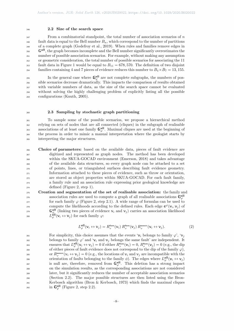
2.2 Size of the search space246

From a combinatorial standpoint, the total number of association scenarios of n247

fault data is equal to the Bell number Bn, which correspond to the number of partitions248

of a complete graph (Godefroy et al., 2019). When rules and families remove edges in249

Gall, the graph becomes incomplete and the Bell number significantly overestimates the250

number of possible association scenarios. For example, without making any assumption251

or geometric consideration, the total number of possible scenarios for associating the 11252

fault data in Figure 1 would be equal to B11 = 678, 570. The definition of two disjoint253

families containing 4 and 7 pieces of evidence reduces this number to B4×B7 = 13, 155.254

In the general case where Gallϕ are not complete subgraphs, the numbers of pos-255

sible scenarios decrease dramatically. This impacts the comparison of results obtained256

with variable numbers of data, as the size of the search space cannot be evaluated257

without solving the highly challenging problem of explicitly listing all the possible258

configurations (Knuth, 2005).259

2.3 Sampling by stochastic graph partitioning260

To sample some of the possible scenarios, we propose a hierarchical method261

relying on sets of nodes that are all connected (cliques) in the subgraph of realisable262

associations of at least one family Gallϕ . Maximal cliques are used at the beginning of263

the process in order to mimic a manual interpretation where the geologist starts by264

interpreting the major structures.265

Choice of parameters: based on the available data, pieces of fault evidence are266

digitized and represented as graph nodes. The method has been developed267

within the SKUA-GOCAD environment (Emerson, 2018) and takes advantage268

of the available data structures, so every graph node can be attached to a set269

of points, lines, or triangulated surfaces describing fault evidence geometry.270

Information attached to these pieces of evidence, such as throw or orientation,271

are stored as object properties within SKUA-GOCAD. For each fault family,272

a family rule and an association rule expressing prior geological knowledge are273

defined (Figure 2, step 1).274

Creation and segmentation of the set of realisable association: the family and275

association rules are used to compute a graph of all realisable associations Gallϕ276

for each family ϕ (Figure 2, step 2.1). A wide range of formulas can be used to277

compute the likelihoods according to the defined rules. Each edge eϕ(vi, vj) of278

Gallϕ (linking two pieces of evidence vi and vj) carries an association likelihood279

Lallϕ (vi ↔ vj) for each family ϕ:280

Lallϕ (vi ↔ vj) = Rfam

ϕ (vi)Rfam

ϕ (vj)Rassoc

ϕ (vi ↔ vj). (2)

For simplicity, this choice assumes that the events ‘vi belongs to family ϕ’, ‘vj281

belongs to family ϕ’ and ‘vi and vj belongs the same fault’ are independent. It282

ensures that Lallϕ (vi ↔ vj) = 0 if either Rfam

ϕ (vi) = 0, Rfamϕ (vj) = 0 (e.g., the dip283

of either pieces of fault evidence does not correspond to the dip of the family ϕ),284

or Rassocϕ (vi ↔ vj) = 0 (e.g., the locations of vi and vj are incompatible with the285

orientation of faults belonging to the family φ). The edges where Lallϕ (vi ↔ vj)286

is null are, therefore, removed from Gallϕ . This deletion has a strong impact287

on the simulation results, as the corresponding associations are not considered288

later, but it significantly reduces the number of acceptable association scenarios289

(Section 2.2). The major possible structures are then listed using the Bron-290

Kerbosch algorithm (Bron & Kerbosch, 1973) which finds the maximal cliques291

in Gallϕ (Figure 2, step 2.2).292

–8–


step 1 Choice of parameters

Family rulesAssociation rules

Fault evidence

step 4 Display association scenarios and export to geomodeling worklow

step 3 Stochastic fault association and downscaling

step 3.1 Draw one of the possible fault

step 3.2 Apply downscaling

step 3.3 Update graph data structure and remaining maximal cliques

step 2 Creation and segmentation of the possibility graph

step 2.2 List all maximal structures (Bron-Kerbosch)

step 2.1 Compute association likelihoodsusing prior geological knowledgeto form the possibility graph

Possible associations per families

NS

W

E

NS

O

E

NS

O

E

NS

O

E

or or

(only two maximal cliques are shown here but 8 can be found)

While some pieces of evidence have not been assigned to a fault

Figure 2. Sequential stochastic algorithm interpreting the available fault data as distinct

cliques in Gallϕ . (step 1) The algorithm requires input fault interpretations and a set of inter-

pretation rules. (step 2.1) Family and association rules are used to compute the graphs Gallϕ of

all possible associations for each family ϕ. (step 2.2) The potential major structures (maximal

cliques) are detected. (step 3) Iteratively sample some fault objects associating a set of data and

update the graph Gallϕ and its maximal cliques. (step 4) When all the pieces of evidence have

been assigned to fault surfaces, the association scenario can be displayed or used to interpolate or

simulate the fault surface geometry.

–9–


1 2 3 4

0.1

0.2

0.3

0.4

(a) 1 2 3 4

0.1

0.2

0.3

0.4

(b)

Nseg

1 2 3 4

0.1

0.2

0.3

0.4

(c)

Nseg

Pseg(Nseg)

Pseg(Nseg) =Nseg

nbobsPseg(Nseg) =

2 Nseg

nbobs (nbobs+1) Pseg(Nseg) =2 (nbobs+1−Nseg)nbobs (nbobs+1)

Nseg

Pseg(Nseg) Pseg(Nseg)

Figure 3. Three probability mass functions that can be used to draw the number of segments

during the segmentation step: (a) uniform, (b) increasing, and (c) decreasing.

Stochastic fault association: cliques are randomly and sequentially drawn and re-293

moved from the remaining realisable associations until each fault evidence has294

been assigned to a fault. Several strategies can be defined and chosen for this295

sequential random selection of faults. To mimic the interpretation process by296

experts, who tend to first focus on the major structures (e.g., Lines & Newrick,297

2004), we propose to preferentially select large and overall likely faults before298

selecting small and unlikely faults. At each step, the sampling probability of299

a clique F = {vi, ..., vj} depends on the number of nodes |F| and on the mean300

association likelihood Lallϕ (F) as301

Pdraw struct(F) =Lallϕ (F) |F|αdraw∑all cliques

FLallϕ (F) |F|αdraw

, (3)

where αdraw is used to weight the number of fault evidences in the clique (the302

structure containing more nodes are more likely to be drawn when αdraw in-303

creases, see sensitivity study in Appendix 6.2). Other selection strategies using,304

for example, the distance separating the pieces of evidence or their sizes could305

also be used to create large structures.306

Stochastic fault segmentation The maximal clique listing is a way to start the in-307

terpretation in a parsimonious manner by looking at the major potential struc-308

tures. However, these potential major structures can be made of several faults309

or several segments possibly linked by relay zones (e.g., Ferrill et al., 1999;310

Julio et al., 2015a; Manighetti et al., 2015; Peacock & Sanderson, 1991). These311

potential fault segments should be considered to completely explore the uncer-312

tainty space. For this, we propose a simple procedure to split a fault F made313

of |F| pieces of fault evidence into Nseg fault segments; this strategy is called314

downscaling in Julio et al. (2015a, 2015b). For simplicity, the number Nseg is315

drawn randomly in this paper between 1 (no segmentation) and |F| (each piece316

of evidence explains one individual fault segment). This random selection relies317

on a discrete probability distribution called Pseg, which can be either uniform,318

linearly decreasing or increasing (Figure 3.a, b, c, respectively). A sensitivity319

analysis is presented in Appendix 6.2 to show how the choice of Pseg impacts320

the total number of detected structures.321

Fault surface modeling: the outcome of the simulation process is a set of associ-322

ation scenarios, each being represented by an association graph (Figure 4.a).323

Converting the graphs into fault network models (Figure 2, step 4) is beyond324

the scope of this paper. While for simple synthetic cases, fault geometry can be325

approximated using geometrical criteria (for example by ellipses computed from326

–10–


the data, Figure 4.b), determining the tip line and fault geometry from the data327

is non trivial and also prone to uncertainties in the general case.328

In the above simulation method, faults are simulated independently, and the329

possibility of interactions is not considered. Even though branch lines are an ubiquitous330

feature of fault networks, branch lines are difficult to map directly from subsurface data331

(Yielding, 2016). In modeling workflows, branch lines are thus interpreted from the332

nearby fault sticks. For this reason, we consider that each piece of fault evidence can333

belong only to one fault surface, and the nodes corresponding to a selected clique are334

not considered in further simulation steps (Figure 2, step 3.3).335

When fault data are interpreted along parallel two-dimensional seismic lines, an336

extra constraint can be added to prevent fault-fault intersections. The obtained associ-337

ations are then free of branch lineswhich. In the sequential fault association framework,338

after each downscaling step (step 3.2), the edges crossing the simulated fault are re-339

moved from the remaining cliques while updating the data structure (step 3.3). A sim-340

ilar graph problem is solved using the Dynamic Time Warping algorithm (Levenshtein,341

1966) in order to correlate stratigraphic data along wells (Edwards et al., 2018; Lallier342

et al., 2013; Smith & Waterman, 1980). Note that the proposed strategy to avoid343

intersections is applicable only in the presence of fault interpretations made on par-344

allel sections. Extending this constraint to irregularly sampled sparse data could be345

achieved, for example, by using visibility criteria (Holgate et al., 2015).346

3 Application to sparse data from Santos basin, offshore Brazil347

We applied the proposed stochastic fault network simulation method on a natural348

example of faulted structures located in the Santos basin. The Santos Basin is located349

offshore SE Brazil and is one of several salt-bearing passive-margin basins flanking the350

South Atlantic (Jackson et al., 2015).351

The Santos Basin formed as a rift during the Early Cretaceous when the South352

Atlantic began to open (e.g., Meisling et al., 2001). Grabens and half grabens were353

filled by largely Barremian, fluvial-lacustrine deposits, which are overlain by an early-354

to-middle Aptian, carbonate-dominated succession (Jackson et al., 2015). During the355

late Aptian, a thick (up to 2.6 km) salt-rich succession was deposited (see Tvedt356

et al. (2016) and references therein). During the Albian, marine conditions estab-357

lished in the Santos Basin, leading to the deposition of carbonate-dominated succes-358

sion (Ithanhaem Formation). An abrupt increase of the water depth in Santos Basin,359

in Cenomanian–Turonian times, drown the Albian carbonate system as a fine-grained,360

clastic-dominated succession accumulated (Itajai-Acu Formation).361

The growth of the observed faults was activated by the mobilization of the un-362

derlying salt-rich unit (Ariri Formation) (Jackson et al., 2015; Tvedt et al., 2016)., as363

thin-skinned normal faulting systems accommodated the overburden stretching above364

the mobile salt. Previous kinematic analysis (Tvedt et al., 2016) showed that the365

faults grew from Albian to Miocene and from Oligocene to present within Albian Car-366

bonates (Ithanhaem Formation) and within Cenomanian to recent fine-grained clastics367

(Itajai-Acu and Marambia formations),368

From a time-migrated three-dimensional seismic image (see sample section on369

Figure 5.a), we selected a densely faulted area where we interpreted 27 fault surfaces370

(see Figure 5.b and Godefroy et al. (2017)). The modeled zone covers an area of 6 km371

per 6 km and is free of branch lines, simplifying the application of our methodology.372

The lengths of the observed faults range from a few hundred meters to 3.6 km.373

–11–


Scenario 05(b1)

(b3)

(a1)

(a3)

(a2)

(a4)

(b2)

(b3)(b4)

Scenario 06

Scenario 14

Scenario 17

Figure 4. (a) The generated interpretation scenarios are represented by association graphs.

(b) For each clique, a fault surface can be interpolated using the geometry of the fault ev-

idence. Data and generated models can be visualized at: gabrielgodefroy.github.io/

StochasticInterpData/Fig4/Fig4.html

–12–


Given the excellent quality of the seismic image, there is very limited structural374

uncertainty in this interpretation, which is used below as the reference interpreta-375

tion. From this reference model, we extracted sparse fault data along several parallel376

two-dimensional sections to emulate the case of the same area being imaged by two-377

dimensional seismic lines (Figure 5.c,d).378

In the remainder of Section 3, we propose numerical experiments to evaluate the379

consistency of the model space sampled by the proposed simulation method from these380

incomplete data sets. Intuitively, a consistent sampling method should, when appro-381

priately parameterized, retrieve the reference association with the maximum frequency.382

Also, the likelihood to retrieve the reference association should increase as more data383

and correct informative rules are used. However, in practice, the rules may be biased384

because of preferential sampling or wrong analog knowledge, so we will also check for385

the impact of using biased rules on the ability of the method to find the correct associ-386

ation. Finally, in a consistent sampling, the spread of the samples around the reference387

should reduce when more information becomes available. However, checking for the388

latter property is difficult, as the dimension of the problem changes when the number389

of observations changes. Therefore, we first study how the structure of the association390

problem changes with the number of fault data and the degree of information brought391

by geological rules.392

3.1 Synthetic two-dimensional lines393

To quantify the role of a particular geological concept in reducing structural394

uncertainty, we now consider several interpretation rules applied to several data sets395

of increasing density extracted from the reference model. The quality of the 3D seismic396

image used to build the reference model enables to determine whether the reference397

association can be retrieved, and to study the influence of chosen geological rules and398

algorithm parameters on the quality of generated interpretations.399

The multi-scenario association strategy was applied on fault evidence extracted400

along 3, 4, 5, and 6 cross-sections (see Figure 5 and online material). The availability of401

a trustworthy reference fault network model allows us to study the proposed stochastic402

interpretation methodology using a set of restrictive geological rules consistent with403

this reference model. Such an ideal case is unrealistic in actual sparse data settings but404

it enables us to test how the rule choices impact structural interpretation by deleting405

and modifying some of the rules.406

3.2 Association rules407

In the considered data set, faults have approximately a north/south strike and408

can be grouped into two fault families: east- and west-dipping faults. Two fault family409

rules are defined based on the dip direction:410

Rfam

ϕ1(vi) =

{1, if vi dips towards the West,

0, otherwise.

and

Rfam

ϕ2(vi) =

{1, if vi dips towards the East,

0, otherwise.

As seismic lines are oriented east/west, the slope of fault interpretations com-411

pletely determines the family, so there is no uncertainty about which family each piece412

–13–


(a)

(c)

(d)

-2+

2A

mplitu

de

2500 m

(a)

6000 m 6000 m

2.5 s

(b)

West-dipping faultsEast-dipping faults

4 seismic lines: 28 pieces of evidence, 17 east-dipping, 11 west-dipping

6 seismic lines: 41 pieces of evidence, 25 east-dipping,

16 west-dipping

Figure 5. Reference structural model located in the Santos Basin, offshore Brazil. (a) Avail-

able reflection seismic data (courtesy of PGS). (b) Reference fault network. (c, d) Generated

interpreted synthetic parallel two-dimensional seismic lines. An interactive three-dimensional

model is provided as supplementary material, in the form of an HTML page.

–14–


of evidence belongs to. East- and west-dipping are respectively identified in blue and413

red on Figure 5.414

To evaluate the likelihood of associating two fault traces of the same family,415

we first use an association rule that restricts the strike of the generated faults to be416

between N330 (strikemin) and N015 (strikemax) for both families:417

Rorient(vi ↔ vj) =

{1, if the strike between vi and vj is between strikemin and strikemax,

0, otherwise.

Additionally, a uniform association distance rule is created to prevent the inter-418

preted fault lengths from being longest than distmax = 3.5 km, the maximum fault419

length observed in the reference model:420

Rdist(vi ↔ vj) = max(1− dist(vi ↔ vj)

distmax, 0).

Finally, both rules are combined using:421

Rassoc

ϕ (vi ↔ vj) = Rdist(vi ↔ vj)Rorient(vi ↔ vj).

The above association rules are simple and rely only on one orientation and one422

distance criterion; a structural geologist would also use (at least) the length of the fault423

sticks, the fault throw, and the geometric relations between the different observations.424

To assess the impact of conceptual information on the structure of the list of425

realizable associations (Figure 6), we first consider each association rule separately.426

As expected, restrictive rules decreases the number of edges in Gallϕ , hence the number427

of possible association scenarios for each family (see Section 2.2). In the interpreted428

area of interest, faults do not intersect each other, so intersections are also forbidden429

during the simulations. In spite of these rules, going from 4 to 6 seismic sections430

increases both the number of graph nodes (from 28 to 41, see Table 1) and graph431

edges (from 378 to 820), making it more difficult to explore the search space and to432

find the reference fault configuration.433

3.3 Evolution of the number of possible scenarios434

The proposed sampling method may generate the same fault scenario severaltimes. To assess whether the sampler has converged, a common strategy consists ingenerating models until the number of distinct scenarios stabilizes (Pakyuz-Charrier etal., 2019; Thiele et al., 2016). For this, we use the metric Ndiff (l,m) which counts thenumber of differences between any two realizations Gasso

l and Gassom . Ndiff is a special

case of graph edit distance (Sanfeliu & Fu, 1983), in which the only edit operationsare edge insertion and deletion:

Ndiff (l,m) =∑

e∈edgesdl,m(e) (4)

where

dl,m(e) =

0 if the edge e is either present or missing in both G

assol and G

assom ,

1 if not.(5)

–15–


Table 1. Number of pieces of fault evidences, corresponding simulation times and Bell number

for different number of synthetic seismic lines. Simulations were performed using all rules de-

scribed in Section 3.2. Simulations were carried out on a PC with an Intel Xeon CPU E5-2650 v3

@ 2.30GHz with 64GB of RAM; the code is not parallelized.

# seismic

lines

# data... ... in ϕ1 ... in ϕ2 # edges in

ref. model

Bell numbers Run time

(5× 107 real.)

3 25 16 9 2 B25 = 4.6×1018 03h49m

4 28 17 11 5 B28 = 6.1×1021 03h51m

5 35 22 13 13 B35 = 2.8×1029 05h30m

6 41 25 16 19 B41 = 2.3×1036 06h54m

(a) 4 seismic lines

No rule Adding familyrules

Adding orientationrules

Adding distancerules

(b) 6 seismic lines

1

10

100

1000 37813655

2932

1210

1

10

100

1000 820300120

6684

37

47

Num

ber

of e

dges

with

non

-zer

o lik

elih

oods

in the

gra

phs

of a

ll pos

sible

ass

ocia

tions

No rule Adding familyrules

Adding orientationrules

Adding distancerules

= 1

= 2

Figure 6. Number of edges per fault family (ϕ) in the graphs of all possible associa-

tions (Gallϕ ) for evidence extracted along (a) 4 seismic lines, and (b) 6 seismic lines. The in-

tegration of geological rules (Appendix 6.1) reduces the density of the graphs of all possi-

ble associations Gallϕ . The lists of realizable associations can be interactively visualized here:

gabrielgodefroy.github.io/StochasticInterpData/Fig6/html/Fig6.html

–16–


Number of realizations

Num

ber

of d

istin

ct

real

izat

ions 3 lines

4 lines

5 lines

6 lines

3 lines

4 lines

5 lines6 lin

es(a) (b)

Number of realizations

Min

imum

num

ber

of

diff

eren

ces 3 lines

4 lines

5 lines

6 lines

Figure 7. (a) Number of distinct association scenarios obtained from 5 × 107 realizations

from 3, 4, 5, and 6 seismic lines. A plateau is not reached for the case with 5 and 6 seismic lines,

highlighting the very large computational complexity of the problem. (b) Minimum number of

differences to the reference found over the first realizations.

For computational reasons, 5 × 107 realizations were simulated from the fault435

interpretations extracted from 3, 4, 5, and 6 virtual seismic lines, using all the previ-436

ously described rules (Figure 7.a). Simulations run in 3 to 7 hours (see Table 1 for437

details). At the beginning of the simulation, the sampling algorithm shows a near-438

optimal exploration efficiency as it generates only different realizations, whatever the439

data density.440

For the case with 3 seismic lines, the plateau is not yet fully reached but for441

the case with 4 seismic lines, a plateau of 6072 distinct realizations is reached after442

3 × 106 realizations. In both cases, the reference association is found 2026 times and443

3164 times for 3 and 4 seismic lines, respectively. This can be explained by the differ-444

ent information content carried by these data sets (see Figure 6 of the supplementary445

material). When simulating from 5 and 6 seismic lines (35 and 41 fault data, respec-446

tively), the numbers of distinct scenarios is still significantly increasing after 5 × 107447

realizations and the reference association is not found. In both cases, the best scenario448

produced has a number of differences Ndiff equal to 1 (Figure 7.b).449

This numerical experiment shows the difficulty of retrieving the reference asso-450

ciation when the number of pieces of fault evidence is high, even if the chosen rules451

are informative and consistent. Indeed, as discussed in Section 2.2, the combinato-452

rial complexity increases in a non-polynomial way with the number of nodes. As a453

consequence, the dimension of the search space to be explored by the algorithm is454

significantly higher when more data become available. Therefore, the reference model455

(and every realization) becomes diluted in the search space when the number of data456

increases. The difficulty to retrieve the reference model suggests that this dilution457

effect is not compensated by the information content carried by the association rules.458

In principle, the graph edit distance Ndiff for different number of data should be459

normalized depending on the search space size and/or on the number of edges in the460

reference model (1).461

–17–


3 seismic lines 4 seismic lines 5 seismic lines 6 seismic lines

Number of differences ( ) with respect to the number of rules for data extracted along 3/4/5/6 seismic lines

Number of differences ( ) with respect to the shift in the distance rule for data extracted along 3/4/5/6 seismic lines

Number of differences ( ) with respect to the shift in the orientation rule for data extracted along 3/4/5/6 seismic lines



(a1) (a2) (a3) (a4)

(b1) (b2) (b3) (b4)

(c1) (c2) (c3) (c4)

Family rules only Adding

orientation rules

Adding distance rules

Forbid

crossings


orientation rules


Forbid

crossings


orientation rules


Forbid

crossings


orientation rules


Forbid

crossings

-3000 -2000 -1000 0(ref) +1000 +2000 +3000

δerr(m)

-3000 -2000 -1000 0(ref) +1000 +2000 +3000

δerr(m)

-3000 -2000 -1000 0(ref) +1000 +2000 +3000

δerr(m)

-3000 -2000 -1000 0(ref) +1000 +2000 +3000

δerr(m)

αerr-20 -15 -10 -05 0(ref) +20+15+10+05

(deg) αerr-20 -15 -10 -05 0(ref) +20+15+10+05

(deg) αerr-20 -15 -10 -05 0(ref) +20+15+10+05

(deg) αerr-20 -15 -10 -05 0(ref) +20+15+10+05

(deg)

Figure 8. Box plots showing the minimum, mean and maximum number of differences

(Ndiff ) between the simulated association graphs and the reference one. Graphs computed

for sparse data extracted from 3 (a1 − c1) to 6 (a4 − c4) seismic lines. (a1 − a4) The integration

of more geological rules reduces the range of possibilities, corresponding to lower density for the

graphs of all geologically meaningful associations Gallϕ . Falsification of the distance rule (b1 − b4)

and of the orientation rule (c1 − c4). Statistics computed over 5 × 105 realizations.

The experiment shows that the formalism and the chosen metric are favorable462

when relatively few pieces of fault evidence are available. This may seems counter-463

intuitive; however, when pieces of evidence are added, the difficulty to explore a larger464

search space increases in a non-polynomial way, as also observed by Edwards et al.465

(2018) for well correlation.466

3.4 Influence of the chosen geological rules on simulation results467

3.4.1 Impact of the number of rules468

We tested the impact of the chosen numerical rules by successively running simu-469

lations with an increasing number of rules (orientation rule, distance between pieces of470

fault evidence, and forbidding fault intersections). 5× 105 realizations were generated471

from digitized fault evidence extracted along the 3, 4, 5, and 6 seismic lines.472

–18–


To analyze these results, we now consider the number of differences Ndiff (l, ref)473

between each simulated association Gassol and the reference association Gassoref inter-474

preted from the full 3D seismic data set. When the simulations are run with more475

rules (Figure 8.a1 − a4), the minimum, mean, and maximum number of differences476

Ndiff (l, ref) consistently decrease. Moreover, we observe that rules interact with the477

data density on two respects. First, considering a single rule in sparse data settings478

(cases with 3 or 4 sections) yields realizations closer to the reference than considering479

more informative rules in denser data settings (cases with 5 or more sections). This480

can be explained by the non-convergence of the sampler for 5 and 6 sections, as shown481

in Figure 7.a. Second, for a given set of rules, the absolute number of differences from482

the reference increases with the number of data. This is a direct effect of the increasing483

complexity of the search space, and may also be explained by the non-convergence of484

the sampler with 5× 107 realizations for more than 5 seismic lines (Figure 8.a4).485

It would be interesting to weight these distributions by a relative likelihood for486

each particular scenario using the correlation rules. If appropriately chosen, the rules487

should then give a larger weight to the scenarios closer to the reference. However,488

computing such a relative likelihood faces again a normalization challenge, as the489

number of graph edges is generally different for each realization.490

3.4.2 Deliberately selecting biased rules491

In practical geological studies, it would be difficult to come up with appropriate492

parameters for the association rules. Therefore, we tested the impact of choosing er-493

roneous geological concepts during structural interpretation: the orientations defining494

the associations rules were shifted by an angle αerr and the distance distmax defining495

the distance association rule was offset by δerr. The mathematical expressions for the496

falsified rules are given in Appendix 6.1.497

We study the mean number of differences to the reference association (over 5×105498

realizations) according to these inappropriate choices (Figure 8.b,c). Strongly biased499

rules make it impossible to retrieve the reference association from fault evidence sam-500

pled along 3, 4, 5 or 6 seismic lines (Figure 8.b1, b2, c1, c2, b3, b4 and c3, c4, respectively).501

When simulating interpretation scenarios from data extracted along 5 or 6 seismic sec-502

tions, the reference scenario is never retrieved.503

In the case of the distance rule, if δerr is negative, no association is allowed,504

yielding a collapse of the ensemble of associations. Such a collapse clearly highlights505

an inconsistency between the rules and the spacing of the synthetic data. On the506

other hand, if the distance rule is more permissive than the reference one (i.e., δerr is507

positive), then the minimum, mean, and maximum numbers of error increase for all508

number of seismic lines.509

The effect of changing the orientation rule is not as dramatic, but for the cases510

with 5 and 6 seismic lines, the deviation from the reference rules leads to a slight511

increase of the mean number of errors.512

4 Discussion and ways forward513

4.1 On uncertainty and objectivity514

A major difference between the proposed approach and the expert-based man-515

ual interpretation is the intrinsic ability of the former to generate several scenarios,516

whereas most of the latter tend to end up with one deterministic solution. A reason is517

–19–


that interpretation exercises are taught as a deterministic activity in the vast major-518

ity of university courses: the general expectation, in surface or subsurface mapping,519

is to produce only the most likely scenario or model. This is shown even in exper-520

iments assessing the interpretation uncertainty, which ask a set of geoscientists to521

produce one interpretation each Bond2007, Bond2015b, Schaaf2019. Cognitive biases522

also explain the difficulty of one to work with multiple hypotheses Chamberlin1890,523

Wilson2019, which is a possible explanation for interpretation bias Bond2007. The ad-524

vent of computer-based methods makes it easier to explore aleatory uncertainties by525

perturbing a reference model see Wellmann2018 and references therein, but addressing526

epistemic uncertainties is more challenging as it requires to formalize the geological527

concepts. The graph-based sampling method proposed in this paper clearly belongs528

to this latter class of methods.529

A major difference between the proposed approach and the expert-based manual530

interpretation is the intrinsic ability of the former to generate scenarios, whereas most531

of the latter tends to end up with deterministic solution. Geoscience is a discipline532

where uncertainty is a key component (Frodeman, 1995) and geoscientists and inter-533

preters are exposed to uncertainty from their first university courses. However, there534

is a large loss between how geologists see uncertainty and what is often produced as535

a result of their work. This is shown even in experiments assessing the interpretation536

uncertainty, which ask a set of geoscientists to produce one interpretation each (Bond537

et al., 2007; Bond, 2015; Schaaf & Bond, 2019). In most studies, a single determinis-538

tic structural model is produced, and structural uncertainty are communicated in the539

form of reports and diagrams. Cognitive biases also explain the difficulty of one to540

work with a large number of hypotheses in parallel (Chamberlin, 1890; Wilson et al.,541

2019). Cognitive biases have been demonstrated experimentally (Kahneman, 2011)542

and are a possible explanation for interpretation bias (Bond et al., 2007). The advent543

of computer-based methods makes it easier to explore aleatory uncertainties by per-544

turbing a reference model (see Wellmann & Caumon, 2018, and references therein),545

but addressing epistemic uncertainties is more challenging as it requires to formalize546

the geological concepts. The graph-based sampling method proposed in this paper547

clearly belongs to this latter class of methods.548

A second major difference with classical fault interpretation is that our approach549

relies on the interpreter to explicitly formulate and organize elementary association550

rules, whereas expert based knowledge is seldom explicitly described. The order by551

which we processed and combined the rules is driven in part by mathematical and al-552

gorithmic convenience, and we do not claim it to be fully objective. Indeed, geological553

interpretation always depends on the current state of knowledge and experience of an554

interpreter, on some model assumptions, and on the tools used during the interpre-555

tation (Bond et al., 2007; Chamberlin, 1890; Frodeman, 1995; Wellmann & Caumon,556

2018). Nonetheless, as compared to classical expert-based interpretation, we see the557

general approach proposed in this paper as a step towards making the interpreta-558

tion process more transparent and reproducible by expressing formally the geological559

concepts.560

4.2 On graphs for structural uncertainty assessment561

We see the graph-based method proposed in this paper as a possible way to com-562

plement or generalize structural uncertainty assessment method. It starts from existing563

observations and thus follows the same philosophy as perturbation strategies, which564

consider uncertainties in the location and/or orientation of observations (Lindsay et565

al., 2012; Pakyuz-Charrier et al., 2018; Wellmann et al., 2010) or modeled structures566

(Holden et al., 2003; Lecour et al., 2001; Røe et al., 2014). Our approach starts with-567

out any particular assumption about how to associate incomplete fault observations568

–20–


together. Unlike previous iterative methods (Aydin & Caers, 2017; Cherpeau et al.,569

2010a; Cherpeau & Caumon, 2015), the potential major fault structures are processed570

in the early steps of our algorithm thanks to the maximal clique detection, assuming571

that largest faults are most likely to correspond to many graph nodes. This reproduces572

a classical interpretation process whereby geologists focus on largest structures before573

focusing on smaller objects (e.g., Lines & Newrick, 2004).574

Approaches addressing topological fault network uncertainty have been proposed575

before, using mainly data-driven iterative simulation methods (Aydin & Caers, 2017;576

Cherpeau & Caumon, 2015; Julio et al., 2015b) or object simulation based on stochastic577

point processes (Hollund et al., 2002; Munthe et al., 1994). All data-driven approaches,578

including the method presented herein, can be seen as an efficient way to honor ob-579

servations, which is a notably difficult and time-consuming process when the spacing580

between observations is smaller than the size of the simulated objects. Data-driven581

fault simulations are parsimonious as they only focus on explaining observations, but582

they can significantly under-estimate the number of faults in a given domain. For583

example, the Santos case study clearly shows that the number of simulated faults de-584

creases when less data is used for the same area of interest (Figure 9). Therefore,585

we firmly believe that a stochastic point process should ultimately complement the586

proposed approach to simulate faults that are not directly supported by observations587

(Bonneau et al., 2016; Cherpeau et al., 2010b; Davy et al., 2013; Holden et al., 2003;588

Munthe et al., 1994; Stoyan & Gloaguen, 2011).589

Another line of progress in the graph-based method concerns the management590

fault branch lines. Indeed, even though the chosen reference data set (Figure 5) is free591

of branch lines, fault branching and interactions are ubiquitous in faulted systems, and592

have been extensively studied to understand fault growth (Watterson, 1986; Walsh et593

al., 2002; Nixon et al., 2014; Nicol et al., 2020). The simulation process should be594

extended to represent how faults branch in the fault network while accounting for595

the chronology of the development of the successive fault families. A second oriented596

graph could represent fault branching. while preserving the spatial dependency of fault597

geometry, hierarchy and the fault abutting relationship (as in Aydin & Caers, 2017;598

Cherpeau et al., 2010b).599

4.3 Are the produced interpretations “geologically realistic”?600

Another major difference between expert-based interpretations and the proposed601

method concerns the amount of interpretive concepts used. Interpretation concepts602

typically arise from outcrop or subsurface analog data bases, laboratory and numerical603

models, or on an inference process applied directly to the data at hand. Those con-604

cepts are conveyed in the form of text, sketches and oral presentations. The proposed605

graph-based method calls for formally defining the rules according to each specific606

geological context. In this paper, we only tested relatively simple geological rules in607

order to assess the consistency of the sampling algorithm. If 3-D models were built,608

we could test also their validity by asking a population of geologist to visually inspect609

the models and rate their likelihood. Further studies are clearly needed to help geosci-610

entists defining the numerical interpretation rules corresponding to the interpretation611

concepts. In the case of faulted structures, concepts include choosing fault surface ori-612

entations from analog data sets (Aydin & Caers, 2017), accounting for fault curvature613

and lateral extension, estimating the fault slip (Cherpeau & Caumon, 2015; Røe et614

al., 2014), and evaluating fault segmentation (Julio et al., 2015a; Manighetti et al.,615

2015; Manzocchi et al., 2019). Machine learning could also come into play in this pro-616

cess, either by inferring rule parameters or a posteriori assessing the likelihood of the617

various realizations produced by the sampling method. Training for these approaches618

–21–


could be achieved on multiple manual interpretations (e.g., Schaaf & Bond, 2019) or619

on processed synthetic models (Wu et al., 2019).620

To test the proposed sampler, we started by choosing an ideal case where the621

parameters of simple rules were calibrated directly on a reference model. We acknowl-622

edge that this is never the case in practice where no reference model exists, but this623

allowed us to compare the simulated scenario with a reference. Tests made in Section624

3.4.2 suggest that, when rule parameters are chosen inappropriately, the simulated625

models can show significant bias, and we can expect that this observation would also626

hold for more complex rules. However, such an automatic method has no guarantee to627

produce the same results as several interpretations made by several experts. One rea-628

son is that the sampling method is likely to miss some important aspects of geological629

interpretation. On this regard, we see two main avenues for improvement:630

• First, the methodology does not completely automate the three-dimensional631

structural modeling. Branch lines are not handled and a boundary represen-632

tation of the subsurface is not generated. This makes it difficult to assess the633

likelihood of the generated fault networks using advanced structural analyzes634

such as global displacement analysis (Freeman et al., 2010) or structural restora-635

tion (Gratier & Guillier, 1993). For this, fault geometries should be modeled636

using explicit surfaces (Lecour et al., 2001; Røe et al., 2014) or implicit surfaces637

(Aydin & Caers, 2017; Cherpeau et al., 2010b). Then, the geological formations638

affected by the fault network should be modeled. Generating such geometries639

would also be useful to assess the impact of fault network uncertainty on resource640

assessment (Richards et al., 2015), to incorporate this source of uncertainty in641

geophysical inverse problems (Giraud et al., 2019; Ragon et al., 2018), or to con-642

sider the geological likelihood in a Bayesian inference problem (Caumon, 2010;643

de la Varga & Wellmann, 2016).644

• Second, the graph formalism at this stage only considers pairwise associations645

but does not use the likelihood of associating several pieces of evidence at once.646

This calls for translating geological concepts into numerical rules which apply647

to all fault evidence at once. For example, one could consider the throw dis-648

tribution along fault strike (as in Cherpeau & Caumon, 2015; Freeman et al.,649

1990) or statistical relationships between observed separations and fault size650

(e.g., Gillespie et al., 1992; Torabi & Berg, 2011). The association likelihoods651

should also be updated during the graph-based interpretation to account for the652

expected likelihood of fault-fault interactions.653

4.4 Inverse problem and clustering of structural interpretations654

Stochastic structural modeling enables the generation of large numbers of alter-655

native scenarios (several millions in this work) which can be used as prior informa-656

tion in subsurface inverse problems (see Wellmann and Caumon (2018) and references657

therein). However, the computational times of focal mechanism inversion, flow simu-658

lation, or seismic forward modeling are often incompatible with more than hundreds659

of models. Furthermore, for a human being, it seems difficult to work with more than660

a few alternative scenarios deemed representative of the uncertainties. An effective661

way to address this problem is to use model clustering in model space (e.g., Suzuki662

et al., 2008) or in data space (e.g., Scheidt et al., 2018; Irakarama et al., 2019). A663

challenge, in both cases, comes from the redundancy of models sampled by a particular664

stochastic methods: indeed, simulation methods tend to generate many similar models665

in a priori likely regions of the search space. This redundancy is needed if the models666

also have a large posterior probability, but it can raise efficiency problems when the667

Bayesian updating is strong. The graph-based sampler described in this paper opens668

some avenues to make progress in this area. Indeed, maximal cliques are detected and669

–22–


processed sequentially within the sampling algorithm. Therefore, a hierarchical clus-670

tering of structural scenarios could be generated by applying the method in a recursive671

manner. A possible and simplified outline of such a hierarchical sampling reads: 6.3.672

5 Conclusions673

The proposed graph-based framework helps interpreting alternative fault scenar-674

ios to account for the uncertainty arising while considering sparse fault sample. Prior675

geological knowledge is formalized using numerical rules. The mathematical format of676

the rules eases the communication of the geological concepts used during the interpre-677

tation and makes the structural interpretation process reproducible. Simple geometric678

rules are used in paper, and further developments on integrating more advanced geo-679

logical concepts have been discussed.680

Each scenario is represented by a graph. The automatic interpretation framework681

relies on the detection of the major possible structures in the graphs of all possible682

associations. This strategy mimics the behavior of an interpreter who would start683

by the larger structures. The use of a graph data structure, as compared to a full684

three-dimensional model, leads to a fast simulation process. This enables to perform685

sensitivity studies on the numerical rules and simulation parameters using sparse data686

extracted from a reference model. Converting the graph into a three-dimensional687

model remains a perspective of this framework.688

The presented numerical experiments illustrate the difficulty in retrieving the689

correct association scenario from sparse data. Even if interpretation rules reduce the690

number of scenarios, it seems highly unlikely that a single interpretation is correct.691

When working with subsurface data, uncertainty is the norm and not the exception692

(Frodeman, 1995). These experiments also confirm that the simultaneous use of several693

coherent geological rules reduces the number of distinct simulated scenarios. The694

simulated models are closest (on average) to the reference model and rule falsification695

decreases the likelihood to find a scenario close to the reference one. These experiments696

formally confirmthat, in the interpretation setting defined in this paper, the importance697

of the prior geological knowledge during structural interpretation.698

We also advocate for making geologists aware of structural uncertainties in the699

early stages of their training during geological education (Chamberlin, 1890) . For-700

malizing explicitly the interpretation concepts should ease their communication and701

limit interpretation biases.702

Acknowledgments703

This work was performed in the frame of the RING project (http://ring.georessources.univ-704

lorraine.fr/) at Universite de Lorraine. We would like to thank for their support705

the industrial and academic sponsors of the RING-GOCAD Consortium managed by706

ASGA. Software corresponding to this paper is available to sponsors in the RING707

software package FaultMod2. We also acknowledge Paradigm for the SKUA-GOCAD708

Software and API. The authors are grateful to PGS Investigacao Petrolıfera Limi-709

tada and to Chris A.L. Jackson for providing the Santos Basin reflection seismic data.710

Readers can access the reference structural model and the generated cross-sections711

from : https://doi.org/10.17605/OSF.IO/MP97W.712

–23–


6 Appendices713

6.1 Rules expression714

We give here the numerical formulas and values used to compute the association715

likelihoods Lallϕ (vi ↔ vj) in the case study presented in Section 3.716

No rule If no prior geological knowledge is used, all the associations are assumedequally likely and

Lallϕi

(vi ↔ vj) = 1

for i ∈ {1, 2}.717

Family rule only If only family rules are used, then Rfamϕ (vi) = 1 and

Lallϕi

(vi ↔ vj) = Rfam

ϕi(vi).

In this Santos Basin case study, the family rules rely on the dip orientation of718

the digitized fault evidence, and719

Rfam

ϕ1(vi) =

{1, if the piece of fault evidence vi is dipping toward the West, and

0, otherwise.

As there is no uncertainty on which family the pieces of evidence belong to,720

the rule for the family ϕ2 can be computed from the one for ϕ1: Rfamϕ2

(vi) =721

1−Rfamϕ1

(vi).722

Orientation rules The orientation computed between two pieces of evidence is ac-counted using a rule and combined with the previously defined family rulesusing

Lallϕ (vi ↔ vj) = Rfam

ϕ (vi)Rfam

ϕ (vj)Rassoc

ϕ (vi ↔ vj),

with Rassocϕ (vi ↔ vj) = Rorientϕ being a discrete association rule:723

Rorientϕi=

{1, if the strike orientation between vi and vj is between strikeminϕi

and strikemaxϕi,

0, otherwise,

with strikeminϕ1= 330, strikemaxϕ1

= 15, strikeminϕ2= 145, and strikemaxϕ2

= 195.724

All rules In this last case, a distance rule is also taken into account. The distance725

association likelihood is defined726

Rdistϕ (vi ↔ vj) = max(1− dist(vi ↔ vj)/distmax, 0),

with distmax = 3600 being the dimension (in meter) of the longest fault observedin the area of interest. This association rule is combined with the orientationrule:

Rassoc

ϕ (vi ↔ vj) = Rdistϕ (vi ↔ vj)Rorientϕ (vi ↔ vj).

Rule falsifications In Section 3.4.2, the numerical values used for the orientationand distance rules are falsified to become:

strikeminϕ1= 330 + αerr,

strikemaxϕ1= 15 + αerr,

strikeminϕ2= 145 + αerr,

strikemaxϕ2= 195 + αerr, and

distmax = 3600 + δerr.

–24–


6.2 Sensitivity to scale parameters727

The simulation process is parameterized by a scalar value αdraw and by a prob-728

ability mass function Pseg, which both relate to the fault size and impact the number729

of simulated fault surfaces. Figure 9 exhibits statistics on the number of simulated730

faults, while modifying these two parameters. Statistics are computed over 5× 105 re-731

alizations, with pieces of fault evidence extracted from the Santos Basin model, along732

4 and 6 virtual cross-sections. All of the rules described in Section 3.2 are used for733

these experiments.734

The probability mass function Pseg used to downscale a fault into several seg-735

ments (Figure 3) clearly influences the mean number of simulated faults (Figure 9a2, b2).736

As expected, the use of a linearly increasing density function leads to the simulation of737

more faults as compared to the decreasing function. When the number of fault obser-738

vations increases, this trend becomes significant whereas the variability over the total739

set of realizations increases. For applications which seek to preferentially generate740

parsimonious scenarios in terms of number of faults, the choice of a decreasing mass741

function seems appropriate. In general, however, it seems more relevant to explore the742

search space, so we will choose the uniform mass function for Pseg from now on, as it743

almost spans the same extreme number of faults as with the increasing or decreasing744

mass functions.745

The scalar αdraw defines the likelihood that major structures (containing more746

fault data) are selected earlier during the simulation (Equation 3 and step 3.2 in747

Figure 2). As expected, a negative or a low αdraw increases the number of generated748

fault structures. The mild decrease of this number when αdraw is larger than 1 suggests749

that the other factors tend to naturally limit the appearance of very large fault objects750

which would gather many fault evidences. This emerging behavior is qualitatively751

consistent with highly skewed distributions observed for fracture size distributions752

(Bonnet et al., 2001). In terms of range, choosing αdraw = 2 approximately spans the753

same minimum and maximum number of faults as generated with other values, so we754

will keep a value of 2 in future experiments.755

6.3 Outline of a hierarchical sampling strategy756

We provide here the outline of a hierarchical sampling strategy, and hope it can757

serve as a basis for further research in stochastic structural interpretation:758

1. Define the starting list of realisable associations Gall0 ← Gall and the starting759

index h← 0760

2. Find the maximal cliques of Gallh761

3. Generate Nh scenarios by sampling a possible fault from the maximal cliques.762

Denote as Vnh, nh = 1, . . . , Nh the set of graph vertices corresponding to that763

clique.764

4. For each scenario nh = 1, . . . , Nh:765

(a) Increment the hierarchical level h← h+ 1766

(b) Update the current list of realisable associations: Gallh ← Gall

h−1 \Vnh767

(c) If Gallh still has vertices, go to Step 2, otherwise terminate.768

References769

Alvarez-Gomez, J. A. (2019). Fmc—earthquake focal mechanisms data management,770

–25–


Decreasing Uniform Increasing

( = 2)

( = 2)

Decreasing Uniform Increasing

-8 -4 0 4 8

( = Uniform)

(a1)

(b1)

(a2)

(b2)

-8 -4 0 4 8

( = Uniform)

Num

ber

of

sim

ula

ted

fau

lts

Num

ber

of

sim

ula

ted

fau

lts

Num

ber

of

sim

ula

ted

fau

lts

Num

ber

of

sim

ula

ted

fau

lts4 lines 4 lines

6 lines 6 lines

40

35

30

25

20

40

35

30

25

20

40

35

30

25

20

40

35

30

25

20

Figure 9. Sensitivity of the number of simulated faults to the parameter αdraw (a1, b1) and

to the probability mass function (a2, b2) used while drawing the number of fault segments Pseg.

Statistics computed over 5 × 105 realizations for the cases with 4 (a1, a2) and 6 (b1, b2) seismic

lines.

–26–


cluster and classification. SoftwareX , 9 , 299–307.771

Anquez, P., Pellerin, J., Irakarama, M., Cupillard, P., Levy, B., & Caumon, G.772

(2019, January). Automatic correction and simplification of geological maps773

and cross-sections for numerical simulations. Comptes Rendus Geoscience,774

351 , 48-58. doi: 10.1016/j.crte.2018.12.001775

Aydin, O., & Caers, J. K. (2017). Quantifying structural uncertainty on fault776

networks using a marked point process within a Bayesian framework. Tectono-777

physics, 712 , 101–124. doi: 10.1016/j.tecto.2017.04.027778

Baudon, C., & Cartwright, J. A. (2008). 3D seismic characterisation of an array779

of blind normal faults in the Levant Basin, Eastern Mediterranean. Journal of780

Structural Geology , 30 (6), 746–760. doi: 10.1016/j.jsg.2007.12.008781

Bond, C. (2015). Uncertainty in structural interpretation: Lessons to be learnt.782

Journal of Structural Geology , 74 , 185–200. doi: 10.1016/j.jsg.2015.03.003783

Bond, C., Gibbs, A., Shipton, Z., & Jones, S. (2007). What do you think this is?784

“Conceptual uncertainty”in geoscience interpretation. GSA Today , 17 (11), 4.785

doi: 10.1130/GSAT01711A.1786

Bonneau, F., Caumon, G., & Renard, P. (2016). Impact of a stochastic sequential787

initiation of fractures on the spatial correlations and connectivity of discrete788

fracture networks. Journal of Geophysical Research: Solid Earth, 121 (8),789

5641–5658. doi: 10.1002/2015JB012451790

Bonnet, E., Bour, O., Odling, N. E., Davy, P., Main, I., Cowie, P., & Berkowitz, B.791

(2001). Scaling of fracture systems in geological media. Reviews of geophysics,792

39 (3), 347-383.793

Bron, C., & Kerbosch, J. (1973). Algorithm 457: finding all cliques of an undirected794

graph. Communications of the ACM , 16 (9), 575–577. doi: 10.1145/362342795

.362367796

Caumon, G. (2010). Towards stochastic time-varying geological modeling. Mathe-797

matical Geosciences, 42 (5), 555-569.798

–27–


Chamberlin, T. C. (1890). The method of multiple working hypotheses. Science,799

15 (366), 92–96.800

Cherpeau, N., & Caumon, G. (2015). Stochastic structural modelling in sparse data801

situations. Petroleum Geoscience, 21 (4), 233–247. doi: 10.1144/petgeo2013802

-030803

Cherpeau, N., Caumon, G., Caers, J., & Levy, B. (2012). Method for stochastic in-804

verse modeling of fault geometry and connectivity using flow data. Mathemati-805

cal Geosciences, 44 (2), 147–168. doi: 10.1007/s11004-012-9389-2806

Cherpeau, N., Caumon, G., & Levy, B. (2010a). Stochastic simulation of fault net-807

works from 2D seismic lines. In SEG Expanded Abstracts (Vol. 29, pp. 2366–808

2370). doi: 10.1190/1.3513325809

Cherpeau, N., Caumon, G., & Levy, B. (2010b). Stochastic simulations of fault810

networks in 3d structural modeling. Comptes Rendus Geoscience, 342 (9), 687–811

694. doi: 10.1016/j.crte.2010.04.008812

Davy, P., Le Goc, R., & Darcel, C. (2013). A model of fracture nucleation, growth813

and arrest, and consequences for fracture density and scaling. Journal of Geo-814

physical Research: Solid Earth, 118 (4), 1393–1407. doi: 10.1002/jgrb.50120815

de la Varga, M., & Wellmann, J. F. (2016, August). Structural geologic modeling816

as an inference problem: A Bayesian perspective. Interpretation, 4 (3), SM1-817

SM16. doi: 10.1190/INT-2015-0188.1818

Edwards, J., Lallier, F., Caumon, G., & Carpentier, C. (2018). Uncertainty819

management in stratigraphic well correlation and stratigraphic architec-820

tures: A training-based method. Computers & Geosciences, 111 , 1–17. doi:821

10.1016/j.cageo.2017.10.008822

Emerson. (2018). SKUA-GOCAD. https://www.pdgm.com/products/skua823

-gocad/.824

Ferrill, D. A., Stamatakos, J. A., & Sims, D. (1999). Normal fault corrugation: Im-825

plications for growth and seismicity of active normal faults. Journal of Struc-826

–28–


tural Geology , 21 (8), 1027–1038. doi: 10.1016/S0191-8141(99)00017-6827

Freeman, B., Boult, P. J., Yielding, G., & Menpes, S. (2010). Using empir-828

ical geological rules to reduce structural uncertainty in seismic interpre-829

tation of faults. Journal of Structural Geology , 32 (11), 1668–1676. doi:830

10.1016/j.jsg.2009.11.001831

Freeman, B., Yielding, G., & Badley, M. (1990). Fault correlation during seismic in-832

terpretation. First Break , 8 (3), 87–95. doi: 10.3997/1365-2397.1990006833

Frodeman, R. (1995). Geological reasoning: Geology as an interpretive and historical834

science. Geological Society of America Bulletin, 107 (8), 960–968. doi: 10.1130/835

0016-7606(1995)107〈0960:GRGAAI〉2.3.CO;2836

Gillespie, P., Walsh, J., & Watterson, J. (1992). Limitations of dimension and837

displacement data from single faults and the consequences for data analysis838

and interpretation. Journal of Structural Geology , 14 (10), 1157–1172. doi:839

10.1016/0191-8141(92)90067-7840

Giraud, J., Lindsay, M., Jessell, M., & Ogarko, V. (2019). Towards geologically rea-841

sonable lithological classification from integrated geophysical inverse modelling:842

Methodology and application case. Solid Earth Discussions, 2019 , 1–27. doi:843

10.5194/se-2019-164844

Godefroy, G., Caumon, G., Ford, M., Laurent, G., & Jackson, C. A.-L. (2017).845

A parametric fault displacement model to introduce kinematic control846

into modeling faults from sparse data. Interpretation, 6 (2), 1–48. doi:847

10.1190/int-2017-0059.1848

Godefroy, G., Caumon, G., Laurent, G., & Bonneau, F. (2019). Structural interpre-849

tation of sparse fault data using graph theory and geological rules. Mathemati-850

cal Geosciences.851

Gombert, B., Duputel, Z., Jolivet, R., Doubre, C., Rivera, L., & Simons, M. (2018,852

February). Revisiting the 1992 Landers earthquake: A Bayesian exploration853

of co-seismic slip and off-fault damage. Geophysical Journal International ,854

–29–


212 (2), 839-852. doi: 10.1093/gji/ggx455855

Gratier, J.-P., & Guillier, B. (1993, March). Compatibility constraints on folded856

and faulted strata and calculation of total displacement using computational857

restoration (UNFOLD program). Journal of Structural Geology , 15 (3-5),858

391–402. doi: 10.1016/0191-8141(93)90135-W859

Grose, L., Ailleres, L., Laurent, G., Armit, R., & Jessell, M. (2019). Inversion of ge-860

ological knowledge for fold geometry. Journal of Structural Geology , 119 , 1–14.861

doi: 10.1016/j.jsg.2018.11.010862

Grose, L., Laurent, G., Ailleres, L., Armit, R., Jessell, M., & Cousin-Dechenaud,863

T. (2018). Inversion of structural geology data for fold geometry. Journal of864

Geophysical Research: Solid Earth, 123 (8), 6318–6333. doi: doi.org/10.1029/865

2017JB015177866

Henza, A. A., Withjack, M. O., & Schlische, R. W. (2011). How do the properties867

of a pre-existing normal-fault population influence fault development dur-868

ing a subsequent phase of extension? Journal of Structural Geology , 33 (9),869

1312–1324. doi: 10.1016/j.jsg.2011.06.010870

Holden, L., Mostad, P., Nielsen, B. F., Gjerde, J., Townsend, C., & Ottesen, S.871

(2003). Stochastic structural modeling. Mathematical Geology , 35 (8), 899–914.872

doi: 10.1023/B:MATG.0000011584.51162.69873

Holgate, N., Joldes, G. R., & Miller, K. (2015). Efficient visibility criterion for dis-874

continuities discretised by triangular surface meshes. Engineering analysis with875

boundary elements, 58 , 1–6.876

Hollund, K., Mostad, P., Nielsen, B. F., Holden, L., Gjerde, J., Contursi, M. G., . . .877

Sverdrup, E. (2002). Havana - a fault modeling tool. Norwegian Petroleum878

Society Special Publications, 11 , 157–171.879

Irakarama, M., Cupillard, P., Caumon, G., Sava, P., & Edwards, J. (2019). Apprais-880

ing structural interpretations using seismic data—theoretical elements. Geo-881

physics, 84 (2), N29–N40.882

–30–


Irving, A., Chavanne, E., Faure, V., Buffet, P., & Barber, E. (2010). An uncertainty883

modelling workflow for structurally compartmentalized reservoirs. Geological884

Society, London, Special Publications, 347 (1), 283–299.885

Jackson, C. A.-L., Jackson, M. P., & Hudec, M. R. (2015). Understanding the kine-886

matics of salt-bearing passive margins: A critical test of competing hypotheses887

for the origin of the Albian Gap, Santos Basin, offshore Brazil. Bulletin,888

127 (11-12), 1730–1751.889

Jessell, M., Ailleres, L., De Kemp, E., Lindsay, M., Wellmann, J., Hillier, M., . . .890

Martin, R. (2014). Next generation three-dimensional geologic modeling and891

inversion. Economic Geology , 18 , 261–272.892

Julio, C. (2015). Conditionnement de la modelisation stochastique 3D des reseaux de893

failles (Unpublished doctoral dissertation). Universite de Lorraine.894

Julio, C., Caumon, G., & Ford, M. (2015a). Impact of the en echelon fault connec-895

tivity on reservoir flow simulations. Interpretation, 3 (4), SAC23–SAC34. doi:896

10.1190/INT-2015-0060.1897

Julio, C., Caumon, G., & Ford, M. (2015b). Sampling the uncertainty associated898

with segmented normal fault interpretation using a stochastic downscaling899

method. Tectonophysics, 639 , 56–67. doi: 10.1016/j.tecto.2014.11.013900

Kahneman, D. (2011). Thinking, fast and slow. Macmillan.901

Knuth, D. E. (2005). The Art of Computer Programming, Volume 4: Generating all902

Combinations and Partitions, Fascicle 3. Addison-Wesley Professional.903

Lallier, F., Antoine, C., Charreau, J., Caumon, G., & Ruiu, J. (2013). Manage-904

ment of ambiguities in magnetostratigraphic correlation. Earth and Planetary905

Science Letters, 371 , 26–36. doi: 10.1016/j.epsl.2013.04.019906

Laurent, G., Caumon, G., Bouziat, A., & Jessell, M. (2013, April). A parametric907

method to model 3D displacements around faults with volumetric vector fields.908

Tectonophysics, 590 , 83–93. doi: 10.1016/j.tecto.2013.01.015909

Lecour, M., Cognot, R., Duvinage, I., Thore, P., & Dulac, J.-C. (2001). Mod-910

–31–


elling of stochastic faults and fault networks in a structural uncertainty study.911

Petroleum Geoscience, 7 (S), S31–S42. doi: 10.1144/petgeo.7.S.S31912

Levenshtein, V. I. (1966). Binary codes capable of correcting deletions, insertions,913

and reversals. In Soviet physics doklady (Vol. 10, pp. 707–710).914

Lindsay, M. D., Ailleres, L., Jessell, M. W., de Kemp, E. A., & Betts, P. G. (2012).915

Locating and quantifying geological uncertainty in three-dimensional models:916

Analysis of the Gippsland Basin, southeastern Australia. Tectonophysics, 546 ,917

10–27. doi: 10.1016/j.tecto.2012.04.007918

Lines, L. R., & Newrick, R. T. (2004). Fundamentals of Geophysical Interpretation.919

Society of Exploration Geophysicists. doi: 10.1190/1.9781560801726920

Mai, P. M., Galis, M., Thingbaijam, K. K. S., Vyas, J. C., & Dunham, E. M. (2017,921

September). Accounting for Fault Roughness in Pseudo-Dynamic Ground-922

Motion Simulations. Pure and Applied Geophysics, 174 (9), 3419-3450. doi:923

10.1007/s00024-017-1536-8924

Manighetti, I., Caulet, C., Barros, L., Perrin, C., Cappa, F., & Gaudemer, Y.925

(2015). Generic along-strike segmentation of Afar normal faults, East926

Africa: Implications on fault growth and stress heterogeneity on seismogenic927

fault planes. Geochemistry, Geophysics, Geosystems, 16 (2), 443–467. doi:928

10.1002/2014GC005691929

Mann, C. J. (1993). Uncertainty in geology. In J. C. Davis & U. C. E. Herzfeld930

(Eds.), Computers in geology—25 years of progress (pp. 241–254). Oxford Uni-931

versity Press, Inc.932

Manzocchi, T., Heath, A., Childs, C., Telles, I., & Carneiro, M. (2019). Modelling933

fault zone displacement partitioning for risking across-fault juxtaposition. In934

81st eage conference and exhibition 2019.935

Meisling, K. E., Cobbold, P. R., & Mount, V. S. (2001). Segmentation of an936

obliquely rifted margin, campos and santos basins, southeastern brazil. AAPG937

bulletin, 85 (11), 1903–1924.938

–32–


Munthe, K., Holden, L., Mostad, P., & Townsend, C. (1994). Modelling sub-seismic939

fault patterns using a Marked Point Process. In Ecmor iv-4th european confer-940

ence on the mathematics of oil recovery. doi: 10.3997/2214-4609.201411151941

Nicol, A., Walsh, J., Childs, C., & Manzocchi, T. (2020). The growth of faults. In942

Understanding faults (pp. 221–255). Elsevier.943

Nixon, C. W., Sanderson, D. J., Dee, S. J., Bull, J. M., Humphreys, R. J., & Swan-944

son, M. H. (2014). Fault interactions and reactivation within a normal-fault945

network at Milne Point, Alaska. AAPG Bulletin, 98 (10), 2081–2107. doi:946

10.1306/04301413177947

Osypov, K., Yang, Y., Fournier, A., Ivanova, N., Bachrach, R., Yarman, C. E., . . .948

Woodward, M. (2013). Model-uncertainty quantification in seismic tomogra-949

phy: Method and applications. Geophysical Prospecting , 61 (6), 1114–1134.950

Pakyuz-Charrier, E., Lindsay, M., Ogarko, V., Giraud, J., & Jessell, M. (2018,951

April). Monte Carlo simulation for uncertainty estimation on structural952

data in implicit 3-D geological modeling, a guide for disturbance distri-953

bution selection and parameterization. Solid Earth, 9 (2), 385–402. doi:954

10.5194/se-9-385-2018955

Pakyuz-Charrier, E., Jessell, M., Giraud, J., Lindsay, M., & Ogarko, V. (2019).956

Topological analysis in monte carlo simulation for uncertainty estimation. Solid957

Earth Discussions, 2019 , 1–37. doi: 10.5194/se-2019-78958

Peacock, D., & Sanderson, D. (1991). Displacements, segment linkage and relay959

ramps in normal fault zones. Journal of Structural Geology , 13 (6), 721–733.960

doi: 10.1016/0191-8141(91)90033-F961

Ragon, T., Sladen, A., & Simons, M. (2018). Accounting for uncertain fault geom-962

etry in earthquake source inversions–i: theory and simplified application. Geo-963

physical Journal International , 214 (2), 1174–1190.964

Ramsay, J. G., & Huber, M. I. (1987). The techniques of modern structural geology:965

Folds and Fractures (Vol. 2). Academic Press.966

–33–


Richards, F. L., Richardson, N. J., Bond, C. E., & Cowgill, M. (2015). Interpre-967

tational variability of structural traps: implications for exploration risk and968

volume uncertainty. Geological Society, London, Special Publications, 421 (1),969

7–27. doi: 10.1144/SP421.13970

Riesner, M., Durand-Riard, P., Hubbard, J., Plesch, A., & Shaw, J. H. (2017, May).971

Building Objective 3D Fault Representations in Active Tectonic Settings. Seis-972

mological Research Letters, 88 (3), 831-839. doi: 10.1785/0220160192973

Rivenæs, J. C., Otterlei, C., Zachariassen, E., Dart, C., & Sjøholm, J. (2005). A 3D974

stochastic model integrating depth, fault and property uncertainty for plan-975

ning robust wells, Njord Field, offshore Norway. Petroleum Geoscience, 11 (1),976

57–65. doi: 10.1144/1354-079303-612977

Røe, P., Georgsen, F., & Abrahamsen, P. (2014). An uncertainty model for fault978

shape and location. Mathematical Geosciences, 46 (8), 957–969.979

Rosenbaum, M. S., & Culshaw, M. G. (2003). Communicating the risks arising from980

geohazards. Journal of the Royal Statistical Society: Series A (Statistics in So-981

ciety), 166 (2), 261–270. doi: 10.1111/1467-985X.00275982

Rotevatn, A., Jackson, C. A.-L., Tvedt, A. B., Bell, R. E., & Blækkan, I. (2018, Au-983

gust). How do normal faults grow? Journal of Structural Geology . doi: 10984

.1016/j.jsg.2018.08.005985

Sanfeliu, A., & Fu, K.-S. (1983). A distance measure between attributed relational986

graphs for pattern recognition. IEEE transactions on systems, man, and cyber-987

netics(3), 353–362.988

Schaaf, A., & Bond, C. E. (2019). Quantification of uncertainty in 3-d seismic in-989

terpretation: implications for deterministic and stochastic geomodelling and990

machine learning. Solid earth.991

Schaeffer, S. E. (2007). Graph clustering. Computer science review , 1 (1), 27–64. doi:992

10.1016/j.cosrev.2007.05.001993

Scheidt, C., Li, L., & Caers, J. (2018). Quantifying uncertainty in subsurface sys-994

–34–


tems (Vol. 236). John Wiley & Sons.995

Schneeberger, R., de La Varga, M., Egli, D., Berger, A., Kober, F., Wellmann, F.,996

& Herwegh, M. (2017). Methods and uncertainty estimations of 3-d struc-997

tural modelling in crystalline rocks: a case study. Solid Earth, 8 (5), 987. doi:998

10.5194/se-8-987-2017999

Seiler, A., Aanonsen, S. I., Evensen, G., & Rivenæs, J. C. (2010). Structural sur-1000

face uncertainty modeling and updating using the ensemble Kalman filter. SPE1001

Journal , 15 (04), 1–062. doi: 10.2118/125352-PA1002

Sepulveda, I., Liu, P. L.-F., Grigoriu, M., & Pritchard, M. (2017, September).1003

Tsunami hazard assessments with consideration of uncertain earthquake slip1004

distribution and location: Tsumani Hazard and Uncertain Earthquakes.1005

Journal of Geophysical Research: Solid Earth, 122 (9), 7252-7271. doi:1006

10.1002/2017JB0144301007

Smith, T. F., & Waterman, M. S. (1980). New stratigraphic correlation techniques.1008

The Journal of Geology , 88 (4), 451–457.1009

Stoyan, D., & Gloaguen, R. (2011, August). Nucleation and growth of geological1010

faults. Nonlinear Processes in Geophysics, 18 (4), 529–536. doi: 10.5194/npg-181011

-529-20111012

Suzuki, S., Caumon, G., & Caers, J. (2008). Dynamic data integration for struc-1013

tural modeling: model screening approach using a distance-based model1014

parameterization. Computational Geosciences, 12 (1), 105–119. doi:1015

10.1007/s10596-007-9063-91016

Tal, Y., Hager, B. H., & Ampuero, J. P. (2018, January). The Effects of Fault1017

Roughness on the Earthquake Nucleation Process. Journal of Geophysical1018

Research: Solid Earth, 123 (1), 437-456. doi: 10.1002/2017JB0147461019

Tarantola, A. (2006). Popper, Bayes and the inverse problem. Nature physics, 2 (8),1020

492–494. doi: 10.1038/nphys3751021

Thiele, S. T., Jessell, M. W., Lindsay, M., Wellmann, J. F., & Pakyuz-Charrier, E.1022

–35–


(2016, October). The topology of geology 2: Topological uncertainty. Journal1023

of Structural Geology , 91 , 74-87. doi: 10.1016/j.jsg.2016.08.0101024

Thore, P., Shtuka, A., Lecour, M., Ait-Ettajer, T., & Cognot, R. (2002). Struc-1025

tural uncertainties: Determination, management, and applications. Geophysics,1026

67 (3), 840–852. doi: 10.1190/1.14845281027

Torabi, A., & Berg, S. S. (2011). Scaling of fault attributes: A review. Marine and1028

Petroleum Geology , 28 (8), 1444–1460. doi: 10.1016/j.marpetgeo.2011.04.0031029

Tvedt, A. B., Rotevatn, A., & Jackson, C. A. (2016). Supra-salt normal fault1030

growth during the rise and fall of a diapir: Perspectives from 3D seismic reflec-1031

tion data, Norwegian North Sea. Journal of Structural Geology , 91 , 1–26. doi:1032

10.1016/j.jsg.2016.08.0011033

Walsh, J., Nicol, A., & Childs, C. (2002). An alternative model for the growth of1034

faults. Journal of Structural Geology , 24 (11), 1669–1675. doi: 10.1016/S01911035

-8141(01)00165-11036

Watterson, J. (1986). Fault dimensions, displacements and growth. Pure and Applied1037

Geophysics, 124 (1-2), 365–373.1038

Wellmann, J. F., & Caumon, G. (2018, Nov). 3-D structural geological models:1039

Concepts, methods, and uncertainties. In I. S. C. (Ed) (Ed.), Advances in geo-1040

physics (Vol. 59, p. 1-121). Elsevier. doi: 10.1016/bs.agph.2018.09.0011041

Wellmann, J. F., Horowitz, F. G., Schill, E., & Regenauer-Lieb, K. (2010, July). To-1042

wards incorporating uncertainty of structural data in 3D geological inversion.1043

Tectonophysics, 490 (3-4), 141–151. doi: 10.1016/j.tecto.2010.04.0221044

Wellmann, J. F., Lindsay, M., Poh, J., & Jessell, M. (2014). Validating 3-D struc-1045

tural models with geological knowledge for improved uncertainty evaluations.1046

Energy Procedia, 59 , 374–381. doi: 10.1016/j.egypro.2014.10.3911047

Wilson, C. G., Bond, C. E., & Shipley, T. F. (2019). How can geologic decision mak-1048

ing under uncertainty be improved? Solid earth, 1–34.1049

Wu, X., Geng, Z., Shi, Y., Pham, N., Fomel, S., & Caumon, G. (2019, Octo-1050

–36–


ber). Building realistic structure models to train convolutional neural net-1051

works for seismic structural interpretation. GEOPHYSICS , 1-48. doi:1052

10.1190/geo2019-0375.11053

Yielding, G. (2016). The geometry of branch lines. Geological Society, London, Spe-1054

cial Publications, 439 , SP439–1. doi: 10.1144/SP439.11055

Zakian, P., Khaji, N., & Soltani, M. (2017, October). A Monte Carlo adapted1056

finite element method for dislocation simulation of faults with uncertain1057

geometry. Journal of Earth System Science, 126 (7), 105. doi: 10.1007/1058

s12040-017-0878-z1059

Zehner, B., Borner, J. H., Gorz, I., & Spitzer, K. (2015, June). Workflows1060

for generating tetrahedral meshes for finite element simulations on com-1061

plex geological structures. Computers & Geosciences, 79 , 105-117. doi:1062

10.1016/j.cageo.2015.02.0091063

Zhu, S., Hack, R., Turner, K., & Hale, M. (2003). How far will uncertainty of the1064

subsurface limit the sustainability planning of the subsurface? In Proc. sus-1065

tainable development & management of the subsurface (sdms) conference (pp.1066

5–7).1067

–37–

multi-scenario interpretations from sparse fault evidence

Documents