Working Paper No.81

Impact of economic growth and electricity consumption on

CO2 emissions in BRICS countries: A panel data analysis

Shibalal Meher

Nabakrushna Choudhury Centre for Development Studies, Bhubaneswar (an ICSSR institute in collaboration with Government of Odisha)

June 2021

1

Impact of economic growth and electricity consumption

on CO2 emissions in BRICS countries: A panel data

analysis

Shibalal Meher1

Abstract

This paper examines the impact of economic growth and electricity consumption in BRICS

countries using panel data over the period 1990 to 2014. The variables pass through the

integration test, cross-dependency test, cointegration test and Granger causality test. The

analysis was conducted using Fully Modified Ordinary Least Squares (FMOLS) and

Dynamic Ordinary Least Squares (DOLS) approaches. The results clearly suggests for a long

run relationship of economic growth and electricity consumption with carbon emissions.

There is unidirectional causality running from GDP and electricity consumption to carbon

emissions. It is found that carbon emissions increase more than proportionately with the

increase in electricity consumption. Our findings do not support the expected Kuznets effect

on carbon emissions in BRICS countries. There is declining trend of carbon emissions at the

early stage of development, which begins to rise after the turning point, thereby passing

through a phase of increasing carbon emissions. It is suggested that the BRICS countries,

which have emerged as the growing economies of the world, should make concerted efforts to

develop a carbon reducing policy so as to achieve a sustainable economic growth.

Keywords: Economic growth, electricity consumption, carbon emissions, Environmental

Kuznets Curve, BRICS, FMOLS, DOLS.

1 Professor of Development Studies, Nabakrushna Choudhury Centre for Development Studies, Bhubaneswar.

E-mail: smeher62@rediffmail.com

2

1. Introduction

The world is facing increasing threat of global warming and climate change due to the rising

greenhouse gas2(GHG) emissions as a result of human activity. The Intergovernmental Panel

on Climate Change (IPCC, 2014) maintains that the key factors that lead to increased GHG

emissions are, among others, the increasing economic activity and energy usage. This has

been the major ongoing concern for both the developed and developing countries. While

carbon dioxide (CO2) is the biggest contributor to the problem, there is global effort to

reduce carbon emissions through different forums. While both the developed and developing

countries are responsible for the increase in CO2 emissions, the developing countries are

mostly blamed for the exhaustive use of energy and other resources for their attempt to

increase economic growth.

As the debate surrounds anthropogenic carbon emissions and climate change typifies

sustainable development dilemma, the global climate effort put forward by the Paris

Agreement advocates urgent attention towards carbon mitigation and adaptation strategies

(Adeneye et al., 2021). The increase in carbon emissions is the result of increasing economic

activities, where electricity plays a crucial role, which is produced mostly by fossil fuel

combustion. While economic development is crucial for the emerging economies, it is

noteworthy to assess the impact of economic growth and energy consumption (electricity

consumption) on carbon emissions.

The link among energy consumption, carbon emissions and economic growth has received

considerable attention by both policy makers and researchers, as the achievement of

sustainable economic growth has gradually become a major global concern (Antonakakiset

al., 2017). The interest in this field has been increased by a number of scholars in recent

years. The existing studies in this field can be classified into the following three groups. The

first group consists of studies that investigate the causal links between energy consumption

and economic growth (see, among others, Kraft and Kraft, 1978; Chiou-Wei et al., 2008;

Chontanawat et al., 2008; Huang et al., 2008; Akinlo, 2009; Apergis and Payne, 2009b;

Ghosh, 2009; Payne, 2010; Ozturk, 2010; Eggoh et al., 2011; Joyeux and Ripple, 2011; Al-

Mulali and Sab, 2012; Chu and Chang, 2012; Dagher and Yacoubian, 2012; Shahbaz and

2Greenhouse gases are gases in the Earth's atmosphere that produce the greenhouse effect. Changes in the

concentration of certain greenhouse gases, from human activity (such as burning fossil fuels), increase the risk

of global climate change.

3

Lean, 2012; Abbas and Choudhury, 2013; Bozoklu and Yilanci, 2013; Dergiades et al.,

2013;Yıldırım et al., 2014, Heidari et al., 2015; Saidi and Hammami, 2015; Sbia et al., 2017).

This group of studies focuses on the total energy consumption and a particular country or a

group of countries, although some studies disentangle the energy usage by energy source.

These studies show no conclusive relationship between economic growth and energy

consumption, but provide four alternative hypotheses, viz. growth hypothesis, conservation

hypothesis, feedback hypothesis and neutrality hypothesis3.

The second group of studies concentrates its attention on the relationship between economic

growth and emissions (e.g. Grossman and Krueger, 1991; Dinda, 2004; Stern, 2004; Chang,

2010; Ghosh, 2010; Kijima et al., 2010; Menyah and Wolde-Rufael, 2010a; Ozturk and

Acaravci, 2010; Govindaraju and Tang, 2013; Al- Mulali et al., 2015; Furuoka, 2015; Gao

and Zhang, 2014;Yang and Zhao, 2014; Arvin et al., 2015; Gozgor et al., 2018; Bekun et al.,

2019; Beyene and Kotosz, 2019; Mahembe et al., 2019; Adedoyin et al., 2020). These

studies are fuelled by the Environmental KuznetsCurve (EKC) hypothesis4.Findings of

these studies are once again inconclusive and country or region specific, as in the case of

the energy-growth relationship.

Finally, the third group of studies combines the aforementioned tworelationships and thus

uses a unified framework to identify the links among energy consumption, carbon emissions

and economic growth (e.g. Soytas et al., 2007; Ang, 2008; Apergis and Payne, 2009a;

Halicioglu, 2009; Soytas and Sari, 2009; Zhang and Cheng, 2009; Menyah and Wolde-

Rufael, 2010b;Chang, 2010; Pao and Tsai, 2011; Niu et al, 2011; Wang et al., 2012a,b; Al

Mamun et al., 2014; Asif et al., 2015; Heidari et al., 2015; Wang and Yang, 2015;

Magazzino, 2016; Antonakakis et al., 2017;Ito, 2017; Nguyen and Wongsurawat, 2017; Cai

et al., 2018; Dar and Asif 2018; Phong et al., 2018; Phuong and Tuyen, 2018). Despite the

fact that it is a relatively new area of study, a wealth of literature has emerged, given its

3 The growth hypothesis is supported when there is evidence of unidirectional causality running from energy

consumption to economic growth. In conservation hypothesis, there is causality from economic growth to

energy consumption. The feedback hypothesis presents a bidirectional causality between energy consumption

and economic growth. The neutrality hypothesis suggests no causality between energy consumption and

economic growth. 4 The Environmental Kuznets Curve (EKC) hypothesis postulates an inverted-U-shaped relationship between

economic growth and environmental degradation. That is, the environmental quality deteriorates at the early

stages of economic development /growth and subsequently improves at the later stages (Dinda, 2004).

4

importance to policy makers. Table 1 presents some recent studies relating to energy

consumption, carbon emissions and economic growth.

It is found that there are diverse results relating to the relationship between economic

growth, energy consumption and carbon emission. The diverse results are due to the use

of different models, time periods and countries. Even within the same group of countries

different results are found. Further, not much studies are devoted to the major emerging

economies like BRICS, which are the largest contributor of greenhouse gases.

2. BRICS: An overview

BRICS is an important grouping of countries (Brazil, Russia, India, China and South

Africa) bringing together the major emerging economies from the world. It comprises 42

per cent of the world population, having 23 per cent of the world GDP and over 16 per

cent share in the world trade. The BRICS countries alone contribute 42 per cent of the

carbon emissions (Table 2).They are already among the top emitters of greenhouse gases

in the world largely due to their consumption of fossil fuels. China and India are the first

and third largest greenhouse emitters in the world and Russia, Brazil and South Africa

are not far behind. The emergence of BRICS as not only major economies, but major

greenhouse emitters over last two decades, has made them central to global climate

discussions (Downie and Williams, 2018). After quit of US from the Paris agreement, BRICS

leaders were quick to reaffirm their support for the Paris agreement calling upon the

international community to jointly work towards the implementation of the Paris agreement

on climate change. Since they have emerged as the growing economy in the world and started

playing leading role in the ‘global growth story’, it is realistic to anticipate that they can

continue to act as an engine of global growth and take active part in carbon reduction despite

being the largest emitters of greenhouse gases. In the following, we present a brief discussion

of the trends and growth of per capita carbon emissions, electricity consumption and Gross

Domestic Product (GDP) of the BRICS countries during the period 1990 to 2014.

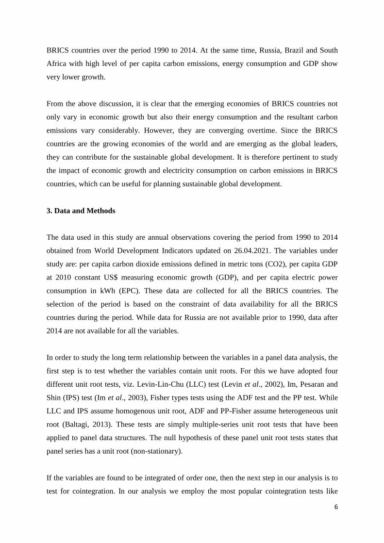
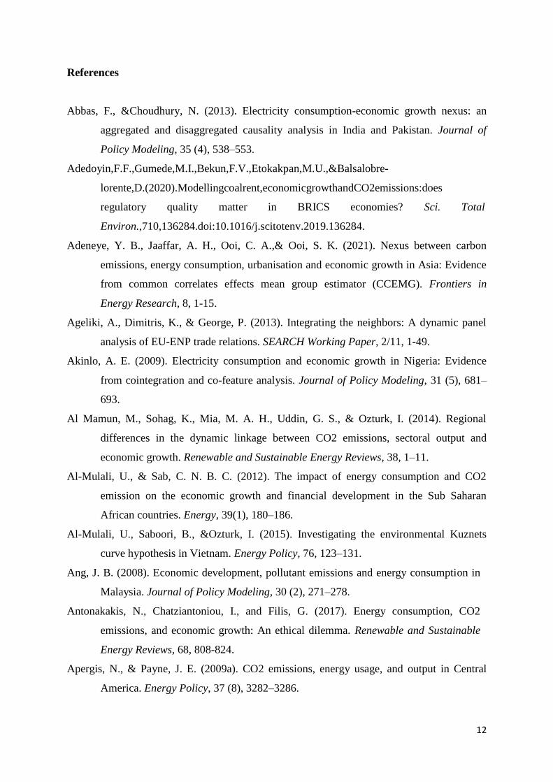
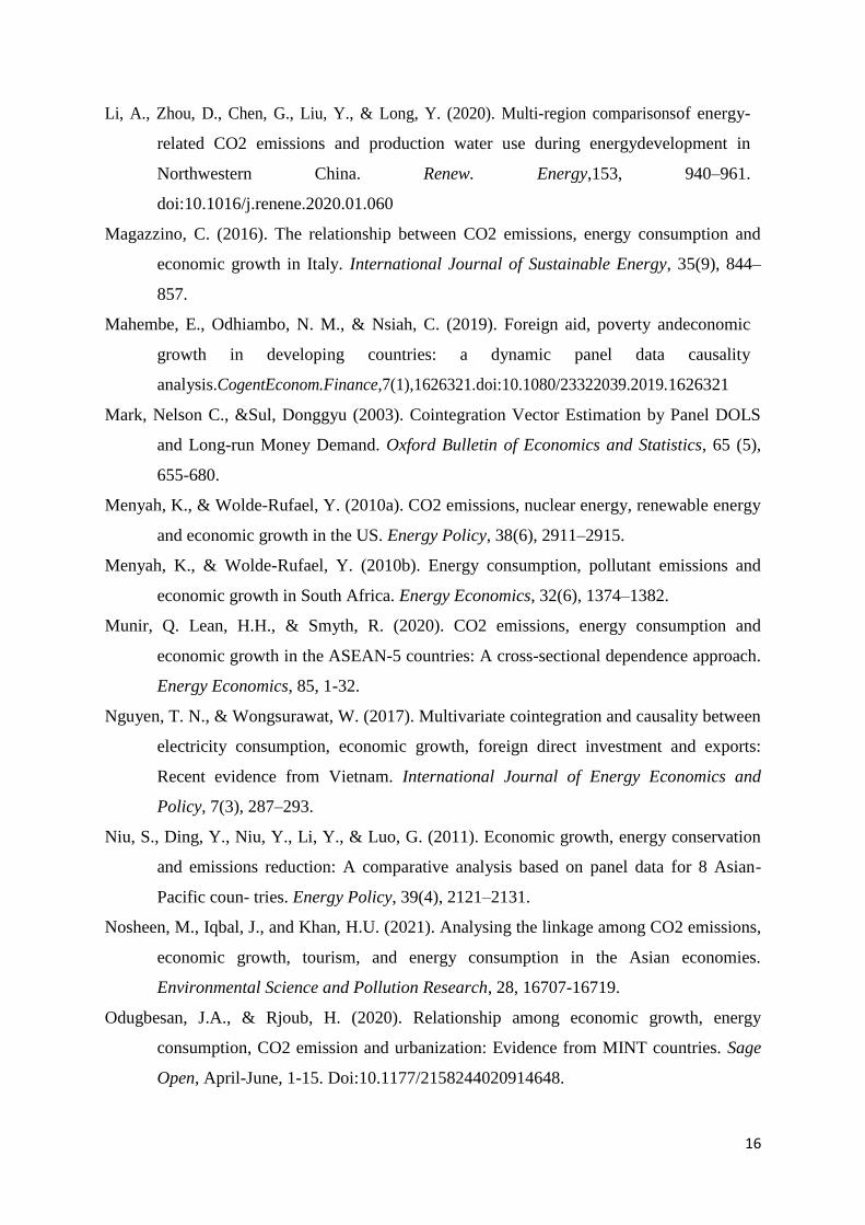
The trends in per capita carbon emissions, electricity consumption and Gross Domestic

Product (GDP) of the BRICS countries are presented in Figures 1 to 3. In Figure 1, the levels

of per capita carbon emissions are plotted for the emerging economies of BRICS for the time

1990 to 2014. While there is increasing trend in per capita carbon emissions for all the

5

BRICS countries over time, Russia is the largest per capita carbon emitting country

throughout the period, followed by South Africa. The per capita carbon emissions of China is

rising speedily after the 1990s and remained over Brazil and India throughout. India’s per

capita carbon emissions is lowest among the BRICS countries during the period. Figure 2

depicts the per capita electricity consumption, which is an important component of energy

consumption in BRICS countries. The level of Russia’s per capita electricity consumption

remained highest throughout the period followed by South Africa. China showed rapid

upward trend in per capita electricity consumption and crossed Brazil in 2007. India’s per

capita electricity consumption though showed increasing trend, remained lowest among the

BRICS countries. Figure 3 depicts the trends in the level of per capita GDP. The level of per

GDP is largest in Brazil, followed by Russia. South Africa’s GDP remains higher than that of

China and India. At the same time, China’s per capita GDP has shown a significant upward

trend, which has increased in an increasing trend. On the other hand, India’s per capita GDP

remained lowest throughout. To summarise, Russia has the highest level of carbon emissions

and electricity consumption, while Brazil has the highest level of per capita GDP during the

period 1990 to 2014. On the other hand, India has not only lowest level of per capita GDP,

but also has lowest per capita carbon emissions and electricity consumption among the

BRICS countries. At the same time, China shows significant upward trends in the three

indicators.

The varying growth of per capita carbon emissions, electricity consumption and GDP among

BRICS countries can be seen from Table 3.China and India have higher annual growth not

only in per capita GDP but also in per capita carbon emissions and electricity consumption

compared to other BRICS countries. Between China and India the growths are much higher

in China than in India. Russia and South Africa having higher level of per capita carbon

emissions and energy consumption, show significantly lower growth in carbon emissions and

electricity consumption compared to other BRICS countries. While there is decline in the

annual growth of carbon emissions in Russia, it is only 1.16 per cent in South Africa.

Similarly the growth of per capita electricity consumption in these two countries is less than

two per cent per annum as compared to 22.74 per cent in China and 10.15 per cent in India.

The growth in per capita GDP of Brazil, Russia and South Africa remains much lower than

China and India. To summarise, China and India, which had low level of per capita carbon

emissions, energy consumption and GDP, show higher annual growth compared to other

6

BRICS countries over the period 1990 to 2014. At the same time, Russia, Brazil and South

Africa with high level of per capita carbon emissions, energy consumption and GDP show

very lower growth.

From the above discussion, it is clear that the emerging economies of BRICS countries not

only vary in economic growth but also their energy consumption and the resultant carbon

emissions vary considerably. However, they are converging overtime. Since the BRICS

countries are the growing economies of the world and are emerging as the global leaders,

they can contribute for the sustainable global development. It is therefore pertinent to study

the impact of economic growth and electricity consumption on carbon emissions in BRICS

countries, which can be useful for planning sustainable global development.

3. Data and Methods

The data used in this study are annual observations covering the period from 1990 to 2014

obtained from World Development Indicators updated on 26.04.2021. The variables under

study are: per capita carbon dioxide emissions defined in metric tons (CO2), per capita GDP

at 2010 constant US$ measuring economic growth (GDP), and per capita electric power

consumption in kWh (EPC). These data are collected for all the BRICS countries. The

selection of the period is based on the constraint of data availability for all the BRICS

countries during the period. While data for Russia are not available prior to 1990, data after

2014 are not available for all the variables.

In order to study the long term relationship between the variables in a panel data analysis, the

first step is to test whether the variables contain unit roots. For this we have adopted four

different unit root tests, viz. Levin-Lin-Chu (LLC) test (Levin et al., 2002), Im, Pesaran and

Shin (IPS) test (Im et al., 2003), Fisher types tests using the ADF test and the PP test. While

LLC and IPS assume homogenous unit root, ADF and PP-Fisher assume heterogeneous unit

root (Baltagi, 2013). These tests are simply multiple-series unit root tests that have been

applied to panel data structures. The null hypothesis of these panel unit root tests states that

panel series has a unit root (non-stationary).

If the variables are found to be integrated of order one, then the next step in our analysis is to

test for cointegration. In our analysis we employ the most popular cointegration tests like

7

Pedroni (1999) and Kao (1999) tests. The Petroni and Kao tests are based on Engle-Granger

(1987) two-step (residual-based) cointegration tests. The tests are implemented on the

residuals obtained from the following regression:

titiitiitiiiti GDPGDPEPCCO ,,2

3,2,1, lnlnln2ln (1)

where Ni ,...,1 and Tt ,...,1 , T is the number of observation over time , N is the number

of countries in the panel, and ti, is the estimated residuals indicating deviations from the

long run relationship.It is assumed that the slope coefficients and the member specific

intercepts can vary across each cross-section. To compute the relevant panel cointegration

test statistics, the cointegration regression in equation (1) is estimated by OLS, for each cross-

section. The panel and group statistics are estimated using the residuals from the

cointegration regression equation (1).

To test for the null hypothesis of no cointegration against the cointegration in the panel,

Pedroni (1999) developed seven cointegration statistics. These are Panel v-Statistic, Panel

rho-Statistic, Panel PP-Statistic, Panel ADF-Statistic, Group rho-Statistic, Group PP-Statistic,

and Group ADF-Statistic. The first four statistics are known as panel cointegration statistics

and are based on the within approach, while the last three statistics are group panel

cointegration statistics and are based on the between approach. In the presence of a

cointegrating relationship, the residuals are expected to be stationary. The panel v-Statistic is

a one sided test where large positive values reject the null of no cointegration. For the

remaining statistics, large negative values reject the null hypothesis of no cointegration.

Besides the Pedroni test we use Kao (1999) test, which is based on the Engle-Granger two-

step procedure, and imposes homogeneity on the members in the panel. The null hypothesis

of no cointegration is tested using an ADF-type test. While Kao test specifies cross-section

specific intercepts and homogenous coefficients, Pedroni tests allow for heterogeneous

intercepts and trend coefficients across cross-sections (Othman and Masih, 2015).

Pedroni’s heterogeneous panel cointegration test and the Kao cointegration test are only able

to indicate whether or not the variables are cointegrated and if a long-run relationship exists

between them. Since they do not indicate the direction of causality, we conduct Granger

8

causality tests on the relationship between variables. The following models are used to test

the Granger panel causality.

ti

K

k

ktiik

K

kktiikkti

K

kikkti

K

kkiiit GDPGDPEPCCOCO ,1

1

,2

11

,1,1

1,1

,11 lnlnln2ln2ln

(2)

ti

K

k

ktiik

K

kktiikkti

K

kikkti

K

kikiit GDPGDPCOEPCEPC ,2

1

,2

21

,2,1

2,1

22 lnln2lnlnln

(3)

tiktiik

K

kktiikkti

K

kikkti

K

kikiit GDPEPCCOGDPGDP ,3,

23

1,3,

13,

133 lnln2lnlnln

(4)

tiktiik

K

kktiikkti

K

kikkti

K

kikiit GDPEPCCOGDPGDP ,4,4

1,4,

14,

2

144

2 lnln2lnlnln

(5)

where i refers to country, t to the time period (t=1,…,T) and k to the lag. The long-run

equilibrium coefficients can be estimated by using single equation estimators such as the

fully modified OLS procedures (FMOLS) developed by Pedroni (2000), the dynamic OLS

(DOLS) estimator from Mark and Sul (2003), the pooled mean group estimator (PMG)

proposed by Pesaran et al. (1999) or by using system estimators as panel VARs estimated

with Generalized Method of Moments (GMM) or Quasi Maximum Likelihood (QML). In our

study, we use both FMOLS and DOLS estimators to estimate the long run coefficients.These

techniques aim to estimate the long run equilibrium relationship among the variables

identified in prior cointegration tests (Othman and Masih, 2015). The FMOLS procedure

accommodates the heterogeneity that is typically present, both in the transitional serial

correlation dynamics and in the long run cointegrating relationships (Papiez, 2013). However,

it is less robust if the data have significant outliers and also have problems in cases where the

residuals have large negative moving average components, which is a fairly common

occurrence in macro time series data (Harris and Sollis, 2003). On the other hand, the DOLS

estimator corrects standard OLS for bias induced by endogeneity and serial correlation on the

leads and lags of the first-differenced regressors from all equations to control for potential

endogeneities (Ageliki et al., 2013).Wagner and Hlouskova (2010) verify that the DOLS

estimator outperforms all other studied estimators, both single equation estimators and system

estimators, even for large samples. However, the DOLS method has the disadvantage of

reducing the number of degrees of freedom, which leads to less reliable estimates. For

cointegrating equation estimations, DOLS and FMOLS aim to estimate the model presented

in equation (1).

9

4. Empirical Findings

Panel Unit Root Tests

Before running for the panel unit tests, we verified the presence of cross-dependency in our

panel dataset. To detect the cross-dependency we applied the most frequently used tests, viz.

Breusch-Pagan LM, Pesaran scaled LM, bias-corrected scaled LM and Pesaran CD. The

results of the tests are presented in Table 4. The results clearly showed the strong presence of

cross-dependency, indicating that panel unit root tests should provide more reliable inference.

We have applied LLC, IPS, and Fisher type tests using ADF and PP to test the integration of

the variables. The results are presented in Table 5. The results show that all the variables, i.e.

lnCO2, lnEPC, lnGDP and lnGDP2, are non-stationary at levels and stationary at first

difference, except in case of lnCO2 which is stationary at level in ADF-Fisher test. This

shows that the variables are integrated of order one, which can be suitable for the

cointegration test.

Cointegration Test

After we found the integration of variables of order one, we proceed for the test of

cointegration of the variables. We applied both the Pedroni and Kao tests of panel

cointegration. The results are presented in Table 6. The null hypothesis of all tests assume no

cointegration between variables. It is observed that the majority of Pedroni’s tests suggest

rejecting the null hypothesis of no cointegration. Out of the 11 tests, seven tests reject the null

hypothesis of no cointegration. Similarly, the Kao cointegration test suggests rejecting null

hypothesis of no cointegration. Therefore, both Pedrini and Kao tests suggest presence of

cointegration among the variables.

Pairwise Granger panel causality test

Though the variables are cointegrated, it is necessary to find out the direction of causality of

the variables. To test the causality of the variables we have used pairwise Granger panel

causality test using stacked test (common coefficients). The result of the Granger causality is

presented in Table 7. It is found that there is unidirectional causality that runs from energy

consumption to carbon emissions, GDP per capita to carbon emissions, and squared GDP to

carbon emissions. This indicates that electricity power consumption and GDP are the factors

influencing carbon emissions in BRICS countries. We have therefore estimated single

10

regression equation with lnCO2 as dependent variable and lnEPC, lnGDP and lnGDP2 as

independent variables to study the impact of these variables on carbon emissions.

Long run equilibrium

We have estimated the long run equilibrium relationship of the single regression equation

with lnCO2 as dependent variable and lnEPC, lnGDP and lnGDP2 as independent variables

as we observe the unidirectional relationship. We have estimated the long run coefficients

using FMOLS and DOLS estimators. Both pooled and grouped mean of the long run

coefficients are estimated using FMOLS and DOLS. It is observed from Table 8that both per

capita electricity consumption and per capita GDP influence per capita carbon emissions

significantly in all the models. The coefficients are elastic, indicating that there is more than

proportionate change in per capita carbon emissions with the change in per capita electric

power consumption and GDP. The coefficients of lnEPC are found to be positive in all the

cases indicating that with the increase in per capita electricity consumption there is increase

in per capita carbon emissions. This is plausible as the BRICS countries generate electricity

mostly by using fossil fuel. At the same time, the estimated coefficients of lnGDP are noticed

to be negative and that lnGDP2 has a positive sign. This shows that economic growth does

not have the expected Kuznets effect on carbon emissions in BRICS countries. At the early

stage of economic growth, carbon emissions cannot be avoided, but when reaching a higher

level, however, circumstances would gradually be improved as the level of development and

welfare improves. The result is however in contradiction to the expected one and thereby

cannot find an inverted U-shaped threshold point. This indicates that in the early stage, there

is declining trendof carbon emissions, but it immediately begins to rise after the turning

point,showing a U-shaped curve instead of inverted U-shaped curve of Kuznets hypothesis.

The above findings are also observed with the individual BRICS countries (Table 9).In all the

five BRICS countries electricity consumption has positive influence on carbon emissions,

indicating that with the increase in electricity consumption there is increase in the carbon

emissions. There is evidence of increase in carbon emissions more than proportionately to the

increase in electricity consumption, with the exception of India. Our findings of different

countries also do not support the expected Kuznets effect on carbon emissions. While the

estimated coefficients of lnGDP are negative, the coefficients of lnGDP2are positive. This is

in contradiction to the inverted U-shaped curve of Kuznets hypothesis. Hence, in these

11

countries, there is declining trend of carbon emissions at the early stage of development, but

begins to rise after the turning point.

5. Conclusions

In this paper the impact of economic growth and electricity consumption on carbon emissions

in BRICS countries has been examined by using panel data over the period 1990 to 2014. The

integration of the variables is verified by using LLC, IPS and Fishers ADF and PP tests. The

long run relationship of the variables are tested by using Pedroni and Kao cointegration test.

The causality of the variables are verified by using Granger causality test. The long run

coefficients are estimated by using FMOLS and DOLS estimators. It is found that the

variables are integrated of order one. All the variables are cointegrated indicating their long

run relationship. There is unidirectional causality running from GDP and electricity

consumption to carbon emissions. The single equation estimation reveals that carbon

emissions is significantly influenced by economic growth and electricity consumption in

BRICS countries. With the increase in electricity consumption the carbon emissions increases

more than proportionately. The economic growth does not have the expected Kuznets effect

on carbon emissions in BRICS countries. In the early stage, there is declining trend, but it

immediately begins to rise after the turning point. Hence, the BRICS countries are passing

through a phase of increasing carbon emissions. As the BRICS countries are the largest

emitters of carbon dioxide, which is the major source of greenhouse gases, they need to

reduce carbon emissions through coordinated efforts. Even though they have shown concern

towards carbon mitigation in different summits, this needs to be transformedinto action. Since

BRICS countries are emerging as the global leaders, they can show the path for a sustainable

economic growth.

12

References

Abbas, F., &Choudhury, N. (2013). Electricity consumption-economic growth nexus: an

aggregated and disaggregated causality analysis in India and Pakistan. Journal of

Policy Modeling, 35 (4), 538–553.

Adedoyin,F.F.,Gumede,M.I.,Bekun,F.V.,Etokakpan,M.U.,&Balsalobre-

lorente,D.(2020).Modellingcoalrent,economicgrowthandCO2emissions:does

regulatory quality matter in BRICS economies? Sci. Total

Environ.,710,136284.doi:10.1016/j.scitotenv.2019.136284.

Adeneye, Y. B., Jaaffar, A. H., Ooi, C. A.,& Ooi, S. K. (2021). Nexus between carbon

emissions, energy consumption, urbanisation and economic growth in Asia: Evidence

from common correlates effects mean group estimator (CCEMG). Frontiers in

Energy Research, 8, 1-15.

Ageliki, A., Dimitris, K., & George, P. (2013). Integrating the neighbors: A dynamic panel

analysis of EU-ENP trade relations. SEARCH Working Paper, 2/11, 1-49.

Akinlo, A. E. (2009). Electricity consumption and economic growth in Nigeria: Evidence

from cointegration and co-feature analysis. Journal of Policy Modeling, 31 (5), 681–

693.

Al Mamun, M., Sohag, K., Mia, M. A. H., Uddin, G. S., & Ozturk, I. (2014). Regional

differences in the dynamic linkage between CO2 emissions, sectoral output and

economic growth. Renewable and Sustainable Energy Reviews, 38, 1–11.

Al-Mulali, U., & Sab, C. N. B. C. (2012). The impact of energy consumption and CO2

emission on the economic growth and financial development in the Sub Saharan

African countries. Energy, 39(1), 180–186.

Al-Mulali, U., Saboori, B., &Ozturk, I. (2015). Investigating the environmental Kuznets

curve hypothesis in Vietnam. Energy Policy, 76, 123–131.

Ang, J. B. (2008). Economic development, pollutant emissions and energy consumption in

Malaysia. Journal of Policy Modeling, 30 (2), 271–278.

Antonakakis, N., Chatziantoniou, I., and Filis, G. (2017). Energy consumption, CO2

emissions, and economic growth: An ethical dilemma. Renewable and Sustainable

Energy Reviews, 68, 808-824.

Apergis, N., & Payne, J. E. (2009a). CO2 emissions, energy usage, and output in Central

America. Energy Policy, 37 (8), 3282–3286.

13

Apergis, N., &Payne, J. E. (2009b). Energy consumption and economic growth in Central

America: evidence from a panel cointegration and error correction model. Energy

Economics, 31 (2), 211–216.

Arvin,M.B.,Pradhan,R.P.,&Norman,N.R.(2015).Transportationintensity,urbanization,

economic growth, and CO2 emissions in the G-20 countries. Util.Pol.,35,50–

66.doi:10.1016/j.jup.2015.07.003

Asif, M., Sharma, R.B., & Adow, A.H.E. (2015). An empirical investigation of the

relationship between economic growth, urbanization, energy consumption, and CO2

emission in GCC countries: A panel data analysis. Asian Social Science, 11(21), 270–

284.

Baltagi, B. (2013). Econometric analysis of panel data. 5th Edn. West

Sussex,Switzerland:JohnWiley&Sons.

Bekun, F.V., Alola, A.A., & Sarkodie, S.A. (2019). Toward a sustainable environment: nexus

between CO2 emissions, resource rent, renewable and non-renewable energy in 16

EU countries, Sci. Total Environ., 657, 1023-1029.

Beyene, S.D., &Kotosz, B. (2019). Testing the environmental Kuznets curve hypothesis: an

empirical study for East African countries. International Journal of Environmental

Studies, 77 (4), 636-654.

Bozoklu, S., &Yilanci, V. (2013). Energy consumption and economic growth for selected

OECD countries: Further evidence from the Granger causality test in the frequency

domain. Energy Policy, 63, 877–881.

Cai, Y., Sam, C. Y., & Chang, T. (2018). Nexus between clean energy consumption,

economic growth and CO2 emissions. Journal of Cleaner Production, 182, 1001–

1011.

Chang, C.C. (2010). A multivariate causality test of carbon dioxide emissions, energy

consumption and economic growth in China. Applied Energy, 87(11), 3533–3537.

Chiou-Wei, S.Z., Chen, C.-F., &Zhu, Z. (2008). Economic growth and energy consumption

revisited–evidence from linear and nonlinear Granger causality. Energy Economics,

30 (6), 3063–3076.

Chontanawat, J., Hunt, L.C., &Pierse, R. (2008). Does energy consumption cause economic

growth? Evidence from a systematic study of over 100 countries. Journal of Policy

Modeling, 30 (2), 209–220.

Chu, H.-P., & Chang, T. (2012). Nuclear energy consumption, oil consumption and economic

growth in G–6 countries: Bootstrap panel causality test. Energy Policy, 48, 762–769.

14

Cowan, W.N., Chang, T., Inglesi-Lotz, R., & Gupta, R. (2014). The nexus of electricity

consumption, economic growth and CO2 emissions in the BRICS countries. Energy

Policy, 66, 359-368.

Dagher, L., & Yacoubian, T. (2012). The causal relationship between energy consumption

and economic growth in Lebanon. Energy policy, 50, 795–801.

Dar, J. A., & Asif, M. (2018). Does financial development improve environmental quality in

Turkey? An application of endogenous structural breaks based cointegration

approach. Management of Environmental Quality: An International Journal, 29(2),

368–384.

Dergiades, T., Martinopoulos, G., &Tsoulfidis, L. (2013). Energy consumption and economic

growth: Parametric and non–parametric causality testing for the case of Greece.

Energy Economics, 36, 686–697.

Dinda, S. (2004). Environmental Kuznets curve hypothesis: A survey. Ecological economics,

49 (4), 431–455.

Downie, C., &Williams, M. (2018). After the Paris agreement: What roles for the BRICS in

global climate governance?. Global Policy, 9 (3), 398-407.

Eggoh, J. C., Bangak´e, C., &Rault, C. (2011). Energy consumption and economic growth

revisited in African countries. Energy Policy, 39 (11), 7408–7421.

Engle, R.F.,and Granger, &C.W.J. (1987). Co-integration and error correction:

Representation, estimation and testing. Econometrica, 55 (2), 251–276.

doi:10.2307/1913236

Furuoka, F. (2015). The CO2 emissions–development nexus revisited. Renewable and

Sustainable Energy Reviews, 51, 1256–1275.

Gao, J., & Zhang, L. (2014). Electricity consumption-economic growth-CO2 emissions

nexus in Sub-Saharan Africa: Evidence from panel cointegration. African

Development Review, 26(2),359–371.doi:10.1111/1467-8268.12087

Ghosh, S. (2009). Electricity supply, employment and real GDP in India: evidence from

cointegration and granger-causality tests. Energy Policy, 37 (8), 2926–2929.

Ghosh, S. (2010). Examining carbon emissions economic growth nexus for India: A

multivariate cointegration approach. Energy Policy, 38(6), 3008–3014.

Govindaraju, V. C., & Tang, C. F. (2013). The dynamic links between CO2 emissions,

economic growth and coal consumption in China and India. Applied Energy, 104,

310–318.

15

Gozgor, G., Lau, C. K. M., & Lu, Z. (2018). Energy consumption and economic growth: New

evidence from the OECD countries. Energy, 153, 27–34.

Grossman, G. M., & Krueger, A. B. (1991). Environmental impacts of the North American

Free Trade Agreement. Tech. rep., NBER working paper.

Halicioglu, F. (2009). An econometric study of CO2 emissions, energy consumption, income

and foreign trade in Turkey. Energy Policy, 37 (3), 1156–1164.

Harris, R., & Sollis, R. (2003). Applied time series modelling and forecasting. Wiley: New

York.

Heidari, H., Katircioğlu, S. T., & Saeidpour, L. (2015). Economic growth, CO2 emissions,

and energy consumption in the five ASEAN countries. International Journal of

Electrical Power & Energy Systems, 64, 785–791.

Huang, B.-N., Hwang, M.-J., &Yang, C.W. (2008). Causal relationship between energy

consumption and GDP growth revisited: a dynamic panel data approach. Ecological

economics, 67 (1), 41–54.

Im, K.S., Pesaran, H.M., & Shin, Y. (2003). Testing for unit roots in heterogeneous panels.

Journal of Econometrics, 115(1), 53–74.

IPCC (2014). Climate change 2014: Synthesis report. Contribution of Working Groups I, II

and III to the Fifth Assessment Report of the Intergovernmental Panel on Climate

Change [Core Writing Team, R. K. Pachauri and L.A. Meyer (eds.)], IPCC, Geneva.

Ito, K. (2017). CO2 emissions, renewable and non-renewable energy consumption, and

economic growth: Evidence from panel data for developing countries. International

Economics, 151, 1–6.

Joyeux, R., & Ripple, R. D. (2011). Energy consumption and real income: a panel

cointegration multi-country study. The Energy Journal, 32 (2), 107.

Kao, C. (1999). Spurious regression and residual-based tests for cointegration in panel data.

Journal of Econometrics, 90, 1–44.

Kijima, M., Nishide, K., &Ohyama, A. (2010). Economic models for the environmental

Kuznets curve: A survey. Journal of Economic Dynamics and Control, 34 (7), 1187–

1201.

Kraft, J., &Kraft, A. (1978). Relationship between energy and GNP. Journal of Energy

Development, 401-403.

Levin, A., Lin, C. F., & James Chu, C.-S. (2002). Unit root tests in panel data: asymptotic

and finite-sample properties. Journal of Econometrics, 108, 1–24.

16

Li, A., Zhou, D., Chen, G., Liu, Y., & Long, Y. (2020). Multi-region comparisonsof energy-

related CO2 emissions and production water use during energydevelopment in

Northwestern China. Renew. Energy,153, 940–961.

doi:10.1016/j.renene.2020.01.060

Magazzino, C. (2016). The relationship between CO2 emissions, energy consumption and

economic growth in Italy. International Journal of Sustainable Energy, 35(9), 844–

857.

Mahembe, E., Odhiambo, N. M., & Nsiah, C. (2019). Foreign aid, poverty andeconomic

growth in developing countries: a dynamic panel data causality

analysis.CogentEconom.Finance,7(1),1626321.doi:10.1080/23322039.2019.1626321

Mark, Nelson C., &Sul, Donggyu (2003). Cointegration Vector Estimation by Panel DOLS

and Long-run Money Demand. Oxford Bulletin of Economics and Statistics, 65 (5),

655-680.

Menyah, K., & Wolde-Rufael, Y. (2010a). CO2 emissions, nuclear energy, renewable energy

and economic growth in the US. Energy Policy, 38(6), 2911–2915.

Menyah, K., & Wolde-Rufael, Y. (2010b). Energy consumption, pollutant emissions and

economic growth in South Africa. Energy Economics, 32(6), 1374–1382.

Munir, Q. Lean, H.H., & Smyth, R. (2020). CO2 emissions, energy consumption and

economic growth in the ASEAN-5 countries: A cross-sectional dependence approach.

Energy Economics, 85, 1-32.

Nguyen, T. N., & Wongsurawat, W. (2017). Multivariate cointegration and causality between

electricity consumption, economic growth, foreign direct investment and exports:

Recent evidence from Vietnam. International Journal of Energy Economics and

Policy, 7(3), 287–293.

Niu, S., Ding, Y., Niu, Y., Li, Y., & Luo, G. (2011). Economic growth, energy conservation

and emissions reduction: A comparative analysis based on panel data for 8 Asian-

Pacific coun- tries. Energy Policy, 39(4), 2121–2131.

Nosheen, M., Iqbal, J., and Khan, H.U. (2021). Analysing the linkage among CO2 emissions,

economic growth, tourism, and energy consumption in the Asian economies.

Environmental Science and Pollution Research, 28, 16707-16719.

Odugbesan, J.A., & Rjoub, H. (2020). Relationship among economic growth, energy

consumption, CO2 emission and urbanization: Evidence from MINT countries. Sage

Open, April-June, 1-15. Doi:10.1177/2158244020914648.

17

Osobajo, O.A., Otitoju, A., Otitoju, M.A., &Oke, A. (2020). The impact of energy

consumption and economic growth on carbon dioxide emissions. Sustainability, 12, 1-

16.

Othman, A. N., & Masih, M. (2015). Do profit and loss sharing (PLS) deposits also affect

PLS financing? Evidence from Malaysia based on DOLS, FMOLS and system GMM

techniques. MPRA Paper No. 65224.

Ozturk, I. (2010). A literature survey on energy–growth nexus. Energy policy, 38 (1), 340-

349.

Ozturk, I., & Acaravci, A. (2010). CO2 emissions, energy consumption and economic growth

in Turkey. Renewable and Sustainable Energy Reviews, 14(9), 3220–3225.

Pao, H.T., & Tsai, C.M. (2011). Modeling and forecasting the CO2 emissions, energy

consumption, and economic growth in Brazil. Energy, 36(5), 2450–2458.

Papiez, M. (2013). CO2 emissions, energy consumption and economic growth in Visegrad

Group countries: A panel data analysis. 31st International Conference on

Mathematical Methods in Economics. 696-701.

Payne, J. E. (2010). A survey of the electricity consumption-growth literature. Applied

energy, 87 (3), 723–731.

Pedroni, P. (1999). Critical values for cointegration tests in heterogeneous panels with

multiple regressors. Oxford Bulletin of Economics & Statistics, 61, 653–670.

Pedroni, P. (2000). Fully modified OLS for the heterogeneous cointegrated panels. Advances

in Econometrics, 15, 93–130.

Pesaran, M. H., Shin, Y., & Smith, R. (1999). Pooled mean group estimator of dynamic

heterogeneous panels. Journal of the American Statistical Association, 94, 621-634.

Phong, L.H., Van, D. T.B., & Bao, H.H.G. (2018). The role of globalization on carbon

dioxide emission in Vietnam incorporating industrialization, urbanization, gross

domestic product per capita and energy use. International Journal of Energy

Economics and Policy, 8(6), 275–283.

Phuong, N.D., & Tuyen, L.T.M. (2018). The relationship between foreign direct investment,

economic growth and environmental pollution in Vietnam: An autoregressive

distributed lags approach. International Journal of Energy Economics and Policy,

8(5), 138–145.

Rahman, A., Murad, S.M.W., Ahmad, F., & Wang, X. (2020). Evaluating the EKC

hypothesis for the BCIM-EC member countries under the belt and road initiative.

Sustainability, 12, 1478, 1-20.

18

Saidi, K., & Hammami, S. (2015). The impact of CO2 emissions and economic growth on

energy consumption in 58 countries. Energy Reports, 1, 62–70.

Salahuddin, M., &Gow, J., 2014. Economic growth, energy consumption and Co2 emissions

in Gulf Cooperation Council countries. Energy, 73, 44–58.

Sbia, R., Shahbaz, M., & Ozturk, I. (2017). Economic growth, financial development,

urbanisation and electricity consumption nexus in UAE. Economic Research-

Ekonomska Istraživanja, 30(1), 527–549.

Shahbaz, M., & Lean, H. H. (2012). Does financial development increase energy

consumption? The role of industrialization and urbanization in Tunisia. Energy

Policy, 40, 473–479.

Soytas, U., &Sari, R. (2009). Energy consumption, economic growth, and carbon emissions:

challenges faced by an EU candidate member. Ecological economics, 68 (6), 1667–

1675.

Soytas, U., Sari, R., &Ewing, B. T. (2007). Energy consumption, income, and carbon

emissions in the United States. Ecological Economics, 62 (3), 482–489.

Stern, D. I. (2004). The rise and fall of the environmental Kuznets curve. World development,

32 (8), 1419–1439.

Wagner, M., & Hlouskova, J. (2010). The performance of panel cointegration methods:

Results from a large scale simulation study. Econometric Reviews, 29(2), 182-223.

Wang, Z., and Yang, L. (2015). Delinking indicators on regional industry development and

carbon emissions: Beijing–Tianjin–Hebei economic band case. Ecological Indicators,

48, 41–48.

Wang, Z., Yin, F., Zhang, Y., & Zhang, X. (2012a). An empirical research on the influencing

factors of regional CO2 emissions: evidence from Beijing city, China. Applied

Energy, 100, 277–284.

Wang, Z.-H., Zeng, H.-L., Wei, Y.-M., Zhang, Y.-X. (2012b). Regional total factor energy

efficiency: an empirical analysis of industrial sector in china. Applied Energy, 97,

115– 123.

Yang, Z., & Zhao, Y. (2014). Energy consumption, carbon emissions, and economic growth

in India: Evidence from directed acyclic graphs. Economic Modelling, 38, 533–540.

Yildirim, E., Sukruoglu, D., & Aslan, A. (2014). Energy consumption and economic growth

in the next 11 countries: The bootstrapped autoregressive metric causality approach.

Energy Economics, 44, 14–21.

19

Zakarya, G.Y., Mostefa, B., Abbes, S.M., &Seghir, G.M. (2015). Factors affecting CO2

emissions in BRICS countries: A panel data analysis. Procedia Economics and

Finance, 26, 114-125.

Zhang, X.P., &Cheng, X.M. (2009). Energy consumption, carbon emissions, and economic

growth in China. Ecological Economics, 68 (10), 2706–2712.

20

Figure 1: Trends in per capita carbon emissions in BRICS countries (metric tons)

Figure 2: Trends in per capita electricity consumptionin BRICS countries (kWh)

Figure 3: Trends in per capita GDPin BRICS countries (constant 2010 US$)

0

5

10

15

20

25

90 92 94 96 98 00 02 04 06 08 10 12 14

Brazil China India

Russia South Africa

0

1,000

2,000

3,000

4,000

5,000

6,000

7,000

90 92 94 96 98 00 02 04 06 08 10 12 14

Brazil China India

Russia South Africa

0

2,000

4,000

6,000

8,000

10,000

12,000

14,000

90 92 94 96 98 00 02 04 06 08 10 12 14

Brazil China India

Russia South Africa

21

Table 1: Empirical studies on the relationship between economic growth, energy consumption and CO2 emissions

Authors

Countries

Period

Data

Methodology

Main findings

Apergis et al. (2010) 19 Developed

and

developing

countries

1984-2007 Real GDP, nuclear and

renewable energy consumption

and CO2 emissions

Panel cointegration and

error correction model NUC ⇒CO2, REC

CO2, REC ⇔GDP,

NUC ⇔GDP.

Chang (2010)

China

1981-2006

Oil, coal, natural gas, electricity

consumption, CO2 emissions

and real GDP

Vector error correction

model

GDP⇒CO2 , OIL and

COAL,

ELEC ⇒GDP and

CO2.

Ozturk and Acaravci

(2010)

Turkey 1968-2005 GDP per capita, CO2 emissions

per capita total energy

consumption per capita and

employment ratio

ARDL coitegration and

Granger causality test

No evidence of EKC.

CO2 and EC does not

cause GDP

Pao and Tsai (2010)

BRICS

1971-2005

GDP per capita, CO2 per capita

and total energy consumption

per capita

Panel cointegration and

VECM

Short-run: EC ⇔CO2,

EC and CO2 ⇒GDP

Long-run: EC ⇔GDP,

CO2 ⇒EC and GDP.

Alam et al. (2012) Bangladesh 1972-2006 GDP per capita, energy

consumptions per capita,

electricity consumption per

capita and CO2 emissions per

capita

ARDL and VECM Short-run: EC ⇒GDP,

ELEC

GDP, EC ⇒CO2,

CO2 ⇒G

Long-run: EC ⇒G,

ELEC ⇔G, EC

⇔CO2, CO2 ⇒G.

22

Jayanthakumaran et

al. (2012)

China, India 1971-2007 GDP per capita, CO2 emissions

per capita and total energy

consumption per capita

ARDL bounds test

approach

Evidence in favour of

EKC,

GDP and EC ⇒CO2

Govindaraju and

Tang (2013)

China, India 1965-2009 GDP per capita, CO2 emissions

per capita and coal consumption

per capita

Cointegration test VECM China:

GDP⇔COALC,

COALC ⇔CO2 ,

GDP⇒CO2 India:

GDP⇔CO2 , COALC

⇔CO2 ,

GDP⇒COALC

Ozcan (2013) 12 Middle East

countries

1990-2008 Real GDP per capita, CO2

emissions per capita and total

energy consumption

Panel cointegration

FMOLS and Panel VECM

Evidence in favour of

EKC (5 out of 12

countries) GDP⇒EC,

EC ⇒CO2.

Saboori and

Sulaiman (2013)

5 ASEAN

countries

1971-2009

Real GDP per capita, CO2

emissions and total energy

consumption

ARDL bounds test

approach to cointegration

and VECM

Mixed results

depending on the

country

Shahbaz et al. (2013)

Indonesia

1975-

2011*

Real GDP per capita, CO2

emissions per capita, total

energy consumption per capita,

financial development and trade

openness per capita

ARDL bounds test

approach to cointegration

and VECM

GDP⇒CO2 ,

EC ⇔CO2

Cowan et al. (2014)

BRICS

1990-2010

Electricity consumption, carbon

dioxide emissions and real GDP

Panel Granger causality

Mixed results

depending on the

country.

Farhani et al. (2014)

Tunisia

1971-2008

Real GDP per capita, CO2

ARDL bounds test

GDP and EC ⇒CO2,

23

emissions per capita, total

energy consumption per capita

and trade openness

approach to cointegration

and VECM CO2 and GDP⇒EC.

Salahuddin and Gow

(2014)

GCC

1980-2012

CO2 emissions, total energy

consumptions, GDP

Panel Granger causality

EC ⇔CO2,

GDP⇒EC,

Heidari et al. (2015)

5 ASEAN

countries

GDP per capita, CO2 emissions

and energy consumption

Panel smooth transition

regression (PSTR)

GDP⇒CO2,

EC ⇒CO2

Zakarya et al. (2015) BRICS 1990-2012 CO2 emissions, primary energy

consumption, FDI net inflow,

GDP per capita

Pedroni cointegration,

Granger causality,Fully

Modified OLS and

Dynamic OLS

CO2⇒ GDP, EC, FDI

Magazzino (2016)

Italy

1970-2006

Real GDP per capita, CO2

emissions and energy

consumption

Toda and Yamamoto,

Granger non-causality

EC ⇔CO2,

GDP⇔CO2

Antonakakis et al.

(2017)

106 countries

1971-2011

Real GDP, CO2 emissions and

energy consumption

Panel Vector Auto

Regression and Impulse

Response function

GDP⇔EC

Cai et al. (2018)

G-7 countries

Real GDP per capita, CO2

emissions and energy

consumption

ARDL Bounds Test

Mixed results

depending on the

country.

Munir et al. (2020)

5ASEAN

countries

1980-2016

GDP, CO2 emissions and energy

consumption

Panel Granger non-

causality

Mixed results

depending on the

country.

Odugbesan and MINT countries 1993-2017 GDP per capita, energy ARDL Bounds test Mixed results

24

Rjoub (2020) consumption, CO2, urbanisation depending on the

country.

Osobajo et al. (2020) 70 countries 1994-2013 CO2 emissions, energy

consumption and GDP growth

Pooled OLS, fixed effects,

Granger causality, Pedroni

and Kao cointegration

GDP growth ⇔CO2,

EC ⇒CO2

Rahman et al. (2020) BCIM-EC

member

countries

1972-2018 CO2 emissions, GDP per capita,

energy use and trade openness

ARDL approach,

Dumitrescu and Hurlin

panel non-causality test

GDP⇒CO2,

GDP2⇒CO2

Nosheen et al. (2021) Asian

economies

1995-2017 GDP, CO2 emissions and energy

consumption

LM bootstrap

cointegration, FMOLS,

DOLS

EC ⇒CO2

25

Table 2: Carbon emissions of BRICS countries (2018)

Countries Carbon emissions (Mt) Share (%)

Brazil 457 1.25

China 10,065 27.52

India 2,654 7.26

Russia 1,711 4.68

South Africa 468 1.28

BRICS total 15,355 41.98

Global total

36,573

100.00

Source: Author’s calculation

Table 3: Annual Growth of per capita carbon emissions, electricity consumption and

GDP in BRICS countries (%)

Country CO2 EPC GDP

Brazil 4.95 5.68 4.23

China 14.29 22.74 22.74

India 8.14 10.15 10.92

Russia -2.50 1.62 5.93

South Africa 1.16 0.69 3.51

CV (%)

109.61

84.13

84.13

Source: Author’s calculation

Table 4: Cross-section dependence tests

Test lnCO2 lnEPC lnGDP lnGDP2

Breusch-Pagan LM 93.07837* 101.6734* 199.7770* 202.3303*

Pesaran scaled LM 18.57689* 20.49880* 42.43543* 43.00637*

Bias-corrected scaled LM 18.47272* 20.39464* 42.33126* 42.90220*

Pesaran CD 5.025022* 8.374784* 14.03875* 14.13878*

Note: Null hypothesis: No cross-section dependence (correlation)

Level of significance: *p 0.01

Source: Author’s calculation

26

Table 5: Panel Unit Root Test

Variables Method Level First Difference

Statistic Prob. Statistic Prob.

LnCO2 Levin, Lin & Chu t -0.94192 0.1731 -6.88788* 0.0000 Im, Pesaran and Shin W-stat -1.49873 0.0670 -5.59981* 0.0000 ADF - Fisher Chi-square 38.5954* 0.0000 50.6329* 0.0000 PP - Fisher Chi-square 15.9300 0.1017 57.0233* 0.0000

LnEPC Levin, Lin & Chu t 0.81963 0.7938 -2.82672* 0.0024 Im, Pesaran and Shin W-stat 2.36577 0.9910 -2.77619* 0.0028 ADF - Fisher Chi-square 4.54731 0.9193 25.2521* 0.0049 PP - Fisher Chi-square 3.04449 0.9804 42.9858* 0.0000

LnGDP Levin, Lin & Chu t -0.62961 0.2645 -3.21954* 0.0006 Im, Pesaran and Shin W-stat 2.90821 0.9982 -3.80253* 0.0001 ADF - Fisher Chi-square 2.25601 0.9940 33.1883* 0.0003 PP - Fisher Chi-square 0.99376 0.9998 41.1165* 0.0000 LnGDP2 Levin, Lin & Chu t 0.42268 0.6637 -3.17258* 0.0008 Im, Pesaran and Shin W-stat 3.55531 0.9998 -3.50277* 0.0002 ADF - Fisher Chi-square 1.38174 0.9993 30.7912* 0.0006 PP - Fisher Chi-square

0.53209

1.0000 38.6038* 0.0000

Note: * denotessignificant at 1% level of significance.

Source: Author’s calculation

Table 6: Cointegration tests for BRICS countries

Methods Test Statistics Prob. Weighted

statistics

Prob.

Pedroni Within dimension v 0.613823 0.2697 -0.509903 0.6949

rho -0.618394 0.2682 -0.394441 0.3466

PP -3.000959* 0.0013 -1.877985** 0.0302

ADF -3.077341* 0.0010 -2.042209** 0.0206

Between dimension rho 0.623927 0.7337

PP -1.688033** 0.0457

ADF -1.648205** 0.0497

Kao

ADF -6.344965*

0.0000

Note: * and ** denote the rejection of null hypothesis of no cointegration at 1%&5%

levelsofsignificance respectively.

Source: Author’s calculation

27

Table 7:Pairwise Granger Causality Tests `

Null Hypothesis: Obs F-Statistic Prob.

LnEPC does not Granger Cause LnCO2 115 11.5815* 3.E-05

LnCO2 does not Granger Cause LnEPC 1.01333 0.3664

LnGDP does not Granger Cause LnCO2 115 6.75380* 0.0017

LnCO2 does not Granger Cause LnGDP 0.04011 0.9607

LnGDP2 does not Granger Cause LnCO2 115 6.77609* 0.0017

LnCO2 does not Granger Cause LnGDP2 0.05822 0.9435

Note: * denotes the rejection of null hypothesis of no cointegration at 1% level of

significance.

Source: Author’s calculation

Table 8: Estimation of long run coefficients (Panel analysis)

FMOLS DOLS

Pooled Grouped Pooled Grouped

LnEPC

1.603609*

(0.0000)

1.823454*

(0.0000)

1.503862*

(0.0000)

1.743941*

(0.0000)

LnGDP

-1.914644*

(0.0000)

-2.546638*

(0.0000)

-1.832993*

(0.0000)

-2.242794*

(0.0000)

LnGDP2

0.071910*

(0.0000)

0.117913*

(0.0000)

0.073070*

(0.0000)

0.092636*

(0.0000)

Adjusted R-

squared

0.979985 0.697082 0.996083 0.492630

Note: * denotessignificant at 1% level of significance

CO2 is the dependent variable

Source: Author’s calculation

Table 9: Estimation of long run coefficients (Individual Countries)

Country FMOLS DOLS

LnEPC LnGDP LnGDP2 LnEPC LnGDP LnGDP2

Brazil 1.444630*

(0.0021)

-1.575679*

(0.0000)

0.049156**

(0.0314)

1.159338*

(0.0056)

-1.569080*

(0.0000)

0.074929*

(0.0072)

China 1.277186*

(0.0000)

-1.429893*

(0.0000)

0.051907*

(0.0000)

3.209670*

(0.0000)

-2.622191*

(0.0000)

-0.020835

(0.2536)

India 0.682084*

(0.0005)

-1.331738*

(0.0000)

0.106532*

(0.0000)

0.596263**

(0.0377)

-1.237869*

(0.0014)

0.105690*

(0.0064)

Russia 5.216111*

(0.0000)

-7.639183*

(0.0000)

0.321745*

(0.0000)

2.587556*

(0.0077)

-3.632193**

(0.0120)

0.156999*

(0.0092)

South Africa 0.497261**

(0.0251)

-0.756699

(0.0562)

0.060223**

(0.0110)

1.166876**

(0.0103)

-2.152637**

(0.0109)

0.146398*

(0.0044)

Note: * &** denote significant at 1%& 5% levels of significance respectively.

CO2 is the dependent variable

Source: Author’s calculation