impact of flavor and higgs physics on theories beyond the ... · the generic relations between...
TRANSCRIPT
Impact of Flavor and HiggsPhysics on Theories Beyond the
Standard Model
Sandro Casagrande
Excellence Cluster UniverseTechnische Universitat Munchen
D-85748 GarchingEmail: [email protected]
Supervised byDr. Martin Gorbahn
GarchingJan 2013


TECHNISCHE UNIVERSITAT MUNCHENExzellenzcluster “Origin and Structure of the Universe”
Impact of Flavor and Higgs Physicson Theories Beyond the Standard
Model
Sandro Casagrande
Vollstandiger Abdruck der von der Fakultat fur Physik der TechnischenUniversitat Munchen zur Erlangung des akademischen Grades eines
Doktors der Naturwissenschaften (Dr. rer. nat.)
genehmigten Dissertation.
Vorsitzende: Univ.-Prof. Dr. Laura Fabbietti
Prufer der Dissertation: 1. TUM Junior Fellow Dr. Martin Gorbahn
2. Univ.-Prof. Dr. Alejandro Ibarra
Die Dissertation wurde am 23.01.2013 bei der Technischen UniversitatMunchen eingereicht und durch die Fakultat fur Physik am 13.02.2013angenommen.


Abstract
Quantum effects of physics beyond the Standard Model receive strong indirect constraintsfrom precisely measured collider observables. In the conceptual part of this thesis, we applythe generic relations between particle interactions in perturbatively unitary theories to cal-culate one-loop amplitudes for flavor physics. We provide template results applicable for anymodel of this class. We also investigate example models that are partly and such that are notperturbatively unitary: the Littlest Higgs model and Randall-Sundrum models. The latterhave a unique coupling structure, which we cover exhaustively. We find strong constraints onthe Randall-Sundrum models and numerically compare those from flavor, electroweak pre-cision, and Higgs physics by performing detailed parameter scans. We observe interestingcorrelations between flavor observables, and we find that constraints from Higgs productionand decays are already competitive.
Zusammenfassung
Quanteneffekte jenseits des Standardmodells sind indirekt, stark durch prazise gemesseneBeschleunigerobservablen beschrankt. Im konzeptionellen Teil dieser Arbeit verwenden wirgenerische Relationen zwischen Teilchenwechselwirkungen perturbativ unitarer Theorien zurBerechnung von Einschleifenamplituden der Flavor-Physik. Wir geben allgemeine Resultate,anwendbar auf alle Modelle dieser Klasse. Wir untersuchen auch Beispielmodelle, welche teil-weise, bzw. nicht perturbativ unitar sind: das Littlest Higgs Modell und Randall-SundrumModelle. Letztere haben eine besondere Kopplungsstruktur, welche wir eingehend besprechen.Wir finden starke Beschrankungen an Randall-Sundrum Modelle und vergleichen solche ausFlavor-, elektroschwacher Prazisions- und Higgs-Physik numerisch mittels detaillierter Para-meterabtastung. Wir finden interessante Korrelationen zwischen Flavor-Observablen und dassBeschrankungen durch Higgs-Produktion und Zerfalle bereits kompetitiv sind.
I

II

Contents
1 Introduction 1
2 The Standard Model of Elementary Particle Physics 52.1 Preliminaries . . . . . . . . . . . . . . . . . . . . . . . . . . . . . . . . . . . . 5
2.1.1 First Principles . . . . . . . . . . . . . . . . . . . . . . . . . . . . . . . 62.1.2 The SM as an Effective Field Theory . . . . . . . . . . . . . . . . . . . 7
2.2 Nomenclature and the Symmetry Breaking Sector . . . . . . . . . . . . . . . 92.3 Quantization and BRST Invariance . . . . . . . . . . . . . . . . . . . . . . . . 132.4 Reasons to Go Beyond . . . . . . . . . . . . . . . . . . . . . . . . . . . . . . . 16
3 Theoretical Classification & Examples of New Physics 213.1 Relations for Perturbatively Unitary Theories . . . . . . . . . . . . . . . . . . 21
3.1.1 The Generic Lagrangian . . . . . . . . . . . . . . . . . . . . . . . . . . 213.1.2 Slavnov-Taylor Identities for Feynman Rules . . . . . . . . . . . . . . 23
3.2 A Little Higgs Model . . . . . . . . . . . . . . . . . . . . . . . . . . . . . . . . 313.2.1 Gauge Structure and T -Parity . . . . . . . . . . . . . . . . . . . . . . 313.2.2 Fermion Sector . . . . . . . . . . . . . . . . . . . . . . . . . . . . . . . 35
3.3 Randall-Sundrum Models . . . . . . . . . . . . . . . . . . . . . . . . . . . . . 403.3.1 Basic Geometry of the Setup . . . . . . . . . . . . . . . . . . . . . . . 403.3.2 The Role of Compactification and Boundary Conditions . . . . . . . . 423.3.3 Fermions in a Curved Background . . . . . . . . . . . . . . . . . . . . 443.3.4 Minimal Randall-Sundrum Model . . . . . . . . . . . . . . . . . . . . . 45
3.3.4.1 Gauge-Boson Sector . . . . . . . . . . . . . . . . . . . . . . . 453.3.4.2 Fermion Sector . . . . . . . . . . . . . . . . . . . . . . . . . . 48
3.3.5 Custodial Randall-Sundrum Model . . . . . . . . . . . . . . . . . . . . 533.3.5.1 Gauge-Boson Sector . . . . . . . . . . . . . . . . . . . . . . . 533.3.5.2 Fermion Sector . . . . . . . . . . . . . . . . . . . . . . . . . . 57
3.3.6 Bulk Profiles and Zero-Mode Spectrum . . . . . . . . . . . . . . . . . 603.3.7 Two Paths to 5d Propagators . . . . . . . . . . . . . . . . . . . . . . . 64
3.3.7.1 Summation over KK Modes . . . . . . . . . . . . . . . . . . . 653.3.7.2 Solution to the 5d EOMs . . . . . . . . . . . . . . . . . . . . 68
3.3.8 Complete Coupling Structure . . . . . . . . . . . . . . . . . . . . . . . 733.3.8.1 Higgs–Fermion Couplings . . . . . . . . . . . . . . . . . . . . 733.3.8.2 Gauge-Boson–Fermion Couplings . . . . . . . . . . . . . . . . 763.3.8.3 Purely Bosonic Couplings . . . . . . . . . . . . . . . . . . . . 783.3.8.4 Four Fermion Couplings . . . . . . . . . . . . . . . . . . . . . 79
4 Aspects of Precision Physics 83
III
CONTENTS
4.1 Flavor Physics . . . . . . . . . . . . . . . . . . . . . . . . . . . . . . . . . . . 834.1.1 Structure of ∆F = 1 Processes in Perturbative Models . . . . . . . . . 84
4.1.1.1 Renormalization of the Generic Z Penguin . . . . . . . . . . 844.1.1.2 Result for the Generic Z Penguin and Box Diagrams . . . . 884.1.1.3 Results for the Littlest Higgs Model with T -parity . . . . . . 93
4.1.2 Constraints and Correlations in the Randall-Sundrum Model . . . . . 944.1.2.1 A Comment on Bounds from Direct Collider Searches . . . . 954.1.2.2 Theoretical Framework and Relevant Formulas . . . . . . . . 954.1.2.3 Modifications of the CKM Matrix . . . . . . . . . . . . . . . 1064.1.2.4 Numerical Analysis of Flavor Observables . . . . . . . . . . . 108
4.2 Electroweak Precision Measurements . . . . . . . . . . . . . . . . . . . . . . . 1244.2.1 Common Observables and Effective Parameters . . . . . . . . . . . . . 124
4.2.1.1 General Discussion and Choice of Input Parameters . . . . . 1244.2.1.2 Effective Parameters for New Physics . . . . . . . . . . . . . 1274.2.1.3 Precision Observables from Z → bb . . . . . . . . . . . . . . 129
4.2.2 Constraints on the Randall-Sundrum Model . . . . . . . . . . . . . . . 1324.2.2.1 General Discussion and Input Parameters . . . . . . . . . . . 1324.2.2.2 Oblique and Universal Contributions . . . . . . . . . . . . . 1324.2.2.3 Bounds from the Zbb Vertex . . . . . . . . . . . . . . . . . . 135
4.3 Higgs Production and Decays at Hadron Colliders . . . . . . . . . . . . . . . 1404.3.1 Results in the SM and Measurements . . . . . . . . . . . . . . . . . . 1404.3.2 Sensitivity of Higgs Production to New Fermions . . . . . . . . . . . . 1484.3.3 Analytic Derivations in the Randall-Sundrum Model . . . . . . . . . . 151
4.3.3.1 General Strategy for Loop Mediated Processes . . . . . . . . 1534.3.3.2 Evaluation of the Two Regulator Limits . . . . . . . . . . . . 1564.3.3.3 UV Regulation as a Decision Criterion . . . . . . . . . . . . 163
4.3.4 Phenomenology of the Randall-Sundrum Model . . . . . . . . . . . . . 1664.3.4.1 Production Channels . . . . . . . . . . . . . . . . . . . . . . 1664.3.4.2 Decays Channels: General Aspects, ZZ, bb . . . . . . . . . . 1734.3.4.3 The Decay into γγ . . . . . . . . . . . . . . . . . . . . . . . . 1774.3.4.4 The Decay into γZ . . . . . . . . . . . . . . . . . . . . . . . 180
5 Conclusion 187
A Collection of Formal Developments and Vertices 191A.1 Collection of STIs for Feynman Rules . . . . . . . . . . . . . . . . . . . . . . 191A.2 Formulas and Vertices of the Littlest Higgs Model . . . . . . . . . . . . . . . 193A.3 Analytic Solutions for the RS Model with One Generation . . . . . . . . . . . 198
B Collection of Numerical and Technical Details 203B.1 Loop Functions . . . . . . . . . . . . . . . . . . . . . . . . . . . . . . . . . . . 203B.2 Numerical Input Parameters . . . . . . . . . . . . . . . . . . . . . . . . . . . . 204B.3 Description of the Parameter Scans in RS Models . . . . . . . . . . . . . . . . 206B.4 Numerical Scans of Higgs Processes in RS Models . . . . . . . . . . . . . . . . 210
Bibliography 222
Acknowledgments 235
IV

Chapter 1
Introduction
We are to admit no more causes of naturalthings than such as are both true andsufficient to explain their appearances.
Isaac Newton
For many decades now, research has been posing the question of truth and sufficiency of theStandard Model of elementary particle physics (SM). The answer to this questions depends onthe very energy at which they are posed. The question of truth has been answered positivelyin collider experiments through the tremendous success of the virtual quantum corrections toprecisely studied processes as they are predicted by the SM alone. Before the program at theCERN Large Hadron Collider (LHC), this applied to all scales relevant to the SM contentexcept its symmetry breaking sector.
Here, we are concerned with theories beyond the SM. The quest for new physics approachesthe question of sufficiency. It is in fact a joint program pursued at the intensity and energyfrontier. The LHC program is now driving it up to unexplored energy scales with its recentlyfinished run at 7 and 8 TeV center-of-mass energy, and hopefully soon even further. In thesearches for direct productions the previously known resonances of the SM were rediscoveredand it seems that the last missing piece at the heart of electroweak symmetry breaking wasconfirmed: a scalar resonance of about 126 GeV mass. Its interactions with other particles areroughly in agreement with the SM Higgs boson but not yet measured with an accuracy thatwould secure this identification. The mass, however, agrees with vacuum stability boundsand could leave the SM as the self-contained theory of non-gravitational forces almost up tothe Planck scale.
We will start this thesis with introducing the SM as the basic low energy theory in chap-ter 2. Our later considerations can be considered as perturbations around this setup. We willalso review the mechanism of electroweak symmetry breaking more closely for later purposesand point out the deficits of the SM, which still lead us to believe that the search for newphysics is promising and ever more pressing.
Each confirmation of the SM as the correct background hypothesis at low — i.e. belowelectroweak — energies carries a potential rejection of the hypothesis of physics beyond theSM. Yet, this depends on the specific model in question, its resonances and the couplingsamongst them. Importantly, most models of new physics carry an intrinsic energy scale (ora few scales), whose variation enhances or diminishes the non-SM effects induced by themodel. Often, this scale is bounded from above by theoretical arguments such as unitar-
1
1. INTRODUCTION
ity, vacuum-stability, triviality, or the more practical assumption of perturbativity. On thephenomenological side, it is important to identify physical observables that are precisely mea-sured, as compared to the typical effects of new physics. Here we are concerned with indirectbounds on new physics, which restrict its virtual contributions through precise measurementof observables at lower energies. Several observables of three classes have been identified thattypically lead to strong bounds. The classes are flavor physics, electroweak precision observ-ables, and since recently also Higgs physics. Given that the constraints are strong, we callthem precision constraints in reference to the specific new physics. This can be either dueto indeed precisely measured observables, or due to large typical differences between the SMand new physics value of the observable, which may have its origin in a symmetry like in thecase of flavor-changing neutral currents (FCNCs).
In order to systematize the study of precision physics for phenomenology beyond theSM, we divide all models of new physics into two classes: perturbatively unitary theoriesand theories that become strongly interacting at a high energy scale. The former theories areequivalent to the class of spontaneously broken gauge theories. Their perturbative high energybehavior implies generic relations among the interactions of particles. We review these genericrelations in order to perform the general renormalization of flavor amplitudes in chapter 4.There, we also give template results that include the unphysical degrees of freedom that arenecessary when working in a renormalizable gauge.
For theories with new strong interactions no such unifying approach exists, and we haveto study the phenomenology model by model. To this end we present in chapter 3 two modelsthat are not perturbatively unitary but partially composite. We review the Littlest Higgsmodel, which is in parts a spontaneously broken gauge theory but has also an explicitlybroken sector. We use it to apply the template flavor results in chapter 4. We investigatewhy the result is feasible, even though the model is partly non-unitary. Later, we also use themodel to exemplify the strength of Higgs production and decays in bounding new physics.
We finally present in chapter 3 one interesting model that we scrutinize in chapter 4 withobservables from all three aforementioned sectors and compare the relative impact and qualityof the resulting bounds. This is the Randall-Sundrum (RS) model, which features a compactextra-dimension with anti de-Sitter geometry. It gives a theoretically appealing explanationof the gauge-hierarchy problem and the hierarchies observed in the quark sector. The modelis especially interesting from a precision physics perspective as it receives relevant constraintsfrom electroweak precision physics, flavor-changing decays and most recently also from Higgsproduction and decays. In combination with the rather small number of free parameters thiscreates a good prospect for the falsifiability of the model.
We introduce the RS model in a minimal setup and a custodially protected version thatlowers the strongest electroweak precision constraints by an enlarged gauge symmetry sectorand a specific fermion embedding. We introduce this model in a very concise notation thatsummarizes the results of the minimal and custodial model and is also extensible to otherenlarged fermion embeddings. This facilitates the comparison of the results in the differentversions of the model. In contrast to most of the literature, the Kaluza-Klein decompositionof 5d fields into 4d states is then done directly in the mass basis. The technique is based on[1] and particularly useful for deriving analytic expressions for couplings between particlesthat allow for a clear understanding. It is also well suited for fast numerical evaluation inparameter scans. We give the full coupling structure and present also results for the 5dpropagators of gauge bosons and fermions. For fermions we have to carefully treat the issueof the Higgs localization in the extra dimension. We derive the fermion propagator for the
2
regularized version of an infrared (IR)-brane Higgs boson based on our work in [2]. This isimportant for the discussion of Higgs physics in the Randall-Sundrum model, where we haveto go into the conceptually demanding question of how to perform loop calculations in thegiven geometrical background.
Before doing so, we start the phenomenological discussion in chapter 4 with flavor con-straints from kaon mixing and direct CP violation in K → ππ. We also study interestingcorrelations between different flavor observables in the kaon sector and present predictionsfor deviations in the Cabibbo-Kobayashi-Maskawa matrix and for the rare Bs decay into twomuons, which was measured recently for the first time. The analyses are based on our workin [3]. We update all numerical input from experimental results and SM calculations to therecent values and improve the discussion of [3] by also taking into account subleading Higgs-induced FCNCs based on results we derived in [4]. It is important to identify the boundsthat affect as few parameters as possible and therefore have good predictivity. We quantita-tively assess the dependence of flavor bounds on all model parameters, most prominently theYukawa sector. A parameter scan with high statistics allows us to find bounds that are morerobust than the typical ones often quoted in the literature. This improves the comparabilityof the bounds to those inferred from electroweak precision observables. We review also thelatter in general in section 4.2 and present updated bounds on the minimal and custodial RSmodel taking into account recent theoretical progress in the SM predictions of Z → bb. Thissection mainly assists to understand the incentive of the custodial RS setup and to benchmarkthe bounds from flavor physics and from Higgs processes.
Higgs physics is then discussed in the remainder of this thesis in section 4.3. There,we investigate how to obtain the correct one-loop result for the RS contribution to Higgsboson production via gluon–gluon fusion and also for subsequent decays to two photons.We carefully treat the interplay of the truncation of very heavy Kaluza-Klein modes, thenecessary regularization of the IR-brane Higgs location in the extra dimension, and the UV-regularization of the theory. We give analytic and exact results for the processes. After that,we numerically investigate them together with all other relevant Higgs boson production anddecay modes, starting from our work on gluon–gluon fusion in [4]. We find that already nowinteresting bounds on the scale of the custodial RS model can be derived from the Higgsboson decay into two photons.
The appendices finally contain technical summaries: detailed lists of further Slavnov-Taylor identities not used in the main text, Feynman rules for the Littlest Higgs model, aninstructive analytic summation of Kaluza-Klein mode contributions to gluon–gluon fusion ina toy RS model, further definitions and numerical input, and a detailed description of themethods used for the RS parameter scans.
3

4

Chapter 2
The Standard Model of ElementaryParticle Physics
We start with an obligatory and short presentation of the Standard Model of elementaryparticle physics (SM). In doing so, we will focus on the aspects that are necessary in thefollowing work and set the relevant notation. We will present the reasons that lead us totrust in the SM as the correct theory of matter and fundamental forces up to the electroweakenergy scale, and moreover, which of its shortcomings give us a strong incentive to studypossible extensions at higher energies.
2.1 Preliminaries
The SM is formulated as a consistent quantum field theory, which has formed through a longhistory of interplay between experiment and theory. It unifies two theoretical branches, theGlashow-Weinberg-Salam theory of electroweak interactions [5–7] and Quantum Chromody-namics (QCD), the theory of strong asymptotically free interactions [8–10].
The theory, as it is formulated today, became widely accepted in the late seventies afterthe confirmation of the quark model [11, 12] by the deep inelastic scattering experiments atSLAC [13], the discovery of weak neutral currents in the Gargamelle experiment at CERN[14] and the observation of jets, particularly three-jets events [15] in the PETRA experimentat DESY. Since then, it has lead to many successful predictions that were later confirmed bydiscoveries, e.g. the existence of the charm quark [16–18] and a third generation of quarksimplied by CP violation in kaon decays [19–21] through the Glashow-Iliopoulos-Maiani (GIM)mechanism. The SM has also passed a multitude of experimental verifications at the level oftesting higher order perturbation theory.
Before entering into theoretical details, we want to highlight one of the main featuresthat the SM exhibits. A fact, most remarkable for the present experimental efforts at theLarge Hadron Collider (LHC), is that the SM can be treated perturbatively beyond the scaleof weak interactions ∼ 100 GeV. This implies that the predictions obtained in perturbationtheory can be reliably tested at the ongoing LHC experiments. Indeed, the latest resultsfrom ATLAS, CMS and LHCb rapidly close in on the SM. The great efforts taken by theseexperimental collaborations culminated in the announcement of the observation of a bosonicresonance of even spin by ATLAS [22] and CMS [29] in July 2012, which is by now establishedat a very high confidence level (CL). We expect that the boson is related to the mechanism of
5

2. THE STANDARD MODEL OF ELEMENTARY PARTICLE PHYSICS
electroweak symmetry breaking found in works by Brout, Englert, Higgs and independentlyby Guralnik, Hagen, and Kibble [37–40]1. This mechanism is responsible for the masses ofthe W and Z bosons, the carriers of the weak force. In the pre-LHC era, the Higgs sectorremained the only sector of the SM whose dynamics were untested. It was the designatedmain goal of the LHC program to investigate this topic. The mass and couplings of the foundparticle comply with the simplest incarnation of the mechanism of electroweak symmetrybreaking and it is likely that what is found is indeed the Higgs particle. Further hints in thisdirection are given by complementary measurements in the final data set of CDF and D0 atTevatron [41]. Increased statistics and more complementary measurements of the particle’sproperties are necessary for a final answer. We will review Higgs physics and the results ofthe measurements in more detail in section 4.3.1.
2.1.1 First Principles
The SM and theories beyond it are based on a few, very general first principles. The formal-ism of fields, particles, and antiparticles is an inevitable consequence of Poincare invariance,quantum mechanics, and the cluster decomposition principle [43]. The latter principle statesthat sufficiently distant experiments should yield uncorrelated results. It is guaranteed if alloperators in the Hamiltonian are evaluated at the same point in space-time. Furthermore,physical observables must commute at space-like separations, what is referred to as locality.This does not necessarily apply to the correlator of the field operators themselves. Causalityis then preserved by the existence of antiparticles. The conservation of probabilities of courserequires a hermitian Hamiltonian and a unitary scattering matrix. This, in turn, guaranteesreal and finite eigenvalues of operators that define physical observables. Finally, stability ofmatter requires the vacuum state of the theory to be bounded from below.
The Poincare group admits representations that can be classified according to their trans-formation property. Since the action itself must be invariant under such transformations, werequire the Lagrangian to transform as a scalar. We know from the Clebsch-Gordan decom-position of coupled representations which couplings include a contribution that transforms asa scalar. Thus, we can use those bilinear, trilinear, etc. combinations of field operators andtheir derivatives that are found to transform as a scalar.
As we already mentioned, it turns out that the SM Lagrangian relies on additional internalsymmetry principles. It is sufficient to consider such symmetries that are generated continu-ously out of the identity and can therefore be composed of infinitesimal transformations withparameters αa as g(α) = 1+iαaT a+O(α2). Those groups are called Lie groups and the spacespanned by the generators T a is the Lie algebra of this group. Only the latter is necessaryfor building the Lagrangian. Since we want the symmetries to act on a finite set of fields,we only need to consider finite dimensional representations of groups with a finite numberof generators and exactly those algebras have been exhaustively classified. After splitting allcontained U(1) factors and dividing the group into its mutually commuting sets, the subsetsare called simple. The classification of Elie Cartan [44] shows that only eight types of suchgroups exist. The SM is based on the direct product of the groups SU(2), SU(3) and anadditional U(1) factor
SU(3)c × SU(2)L × U(1)Y (2.1.1)
1In this thesis, we abbreviate it simply as the Higgs mechanism without implying a value judgment.
6

2.1. PRELIMINARIES
symmetry, with the first group corresponding to strong interactions and the others to elec-troweak interactions.
Other global symmetries such as baryon number B, lepton number L, spatial parity P ,charge conjugation C, and time reversal T may, or may not be conserved. We will discussthe origin of CP violation in the SM in section 2.2. However, the combined transformationCPT is conserved in any quantum field theory [45].
2.1.2 The SM as an Effective Field Theory
The aforementioned feature of perturbativity in the SM holds even up to the Planck scale, thescale where the gravitational coupling becomes strong. More generally, perturbative unitar-ity, which is the bounded high-energy growth of scattering amplitudes order by order in theloop expansion, has an intimate one-to-one correspondence with the fact that the theory isspontaneously broken and renormalizable. A theory is called renormalizable, if all formal di-vergences stemming from ultraviolet (UV) momenta that appear in intermediate calculationsof correlation functions with virtual intermediate particles can be absorbed into a redefini-tion of the fundamental parameters of the bare Lagrangian. The latter is the most generalLagrangian one can conceive under certain space-time and internal symmetry assumptionsand a few other consistency conditions, we mention below. Renormalizability of the SM wasproven by t’Hooft and Veltman [46].
In the modern interpretation of the SM one does not see renormalizability as a necessaryfundamental property, but one rather considers the SM as the effective field theory (EFT)relevant for energies at least up to the electroweak scale. The effects of the heavy particlesφH in extensions of the SM LNP = LSM(φSM) + LH(φH , φSM) can then be systematicallyincorporated in a matching calculation onto the relevant and marginal SM operators, supple-mented with additional irrelevant operators Leff = LSM(φSM) +Lirr(φSM). The latter encodethe effects of the new physics (NP) beyond the SM at energies of physical processes below thematching scale µH , i.e. in the region where the new heavy particles are quasi non-dynamical.We already employed terminology from the classification of operators in the operator prod-uct expansion (OPE). In the OPE one uses the fact that the products of field operatorsA,B, entering Green’s functions, can be expanded in terms of local operators and coefficientfunctions
∫dx e−ik·xA(x)B(0) ≈
k→∞
∑jCj(k)Oj , Cj(k) ∼ k[A]+[B]−[Oj ] , (2.1.2)
where the Wilson coefficients Cj [47] encode the large momentum dependence accordingto the sum of mass dimensions of the operators in square brackets. This property holdsunder renormalization up to logarithmic corrections [48]. The effective operators need tocomply with the global symmetry properties of the left-hand side. Using such expansions,one calculates a matching of all one light-particle irreducible Feynman diagrams with externallight particles and requires them to be the same in the full and in the effective theory. Thisresults in an effective Lagrangian where the operators Oj depend only on light fields. Thecoefficient functions are analytic functions in k/µH in the region relevant for the low energytheory. They can therefore be cast into a series of terms with decreasing importance, wherethe matching procedure determines the constant coefficients
Leff(x) =∑
j
gj
µ[Qj ]−4H
Qj(φSM(x)
). (2.1.3)
7

2. THE STANDARD MODEL OF ELEMENTARY PARTICLE PHYSICS
The remaining momenta are combined with the fields φSM into gauge invariant operators Qj .From their mass dimension, one infers the relative importance due to the suppression withthe high mass scale µH . Here, we have written it out explicitly. The expected scaling of thematrix elements is 〈f |Qj |i〉 ∼ E[Qj ]−4 with the typical energy E of the process i → f . Oncethe matter content is defined, all possible operators compatible with the gauge symmetrygroup SU(3)c×SU(2)L×U(1)Y and [Qj ] ≤ 4 are indeed included in the SM. They are calledmarginal, or relevant depending on whether the equality is fulfilled or not. Integrating outnew heavy degrees of freedom leads to a finite number of operators at any given value of[Qj ] > 4, which are called irrelevant. Working at a given level of precision corresponds toneglecting operators in (2.1.3) with dimensionality higher than a fixed value. Supplementedwith the prescription Qj ≡ 0, if [Qj ] > Dmax, an EFT is predictive, and in a sense triviallyrenormalizable by definition. On the other hand, increasing the required level of precisionalso requires increasing Dmax, and thus further experimental input in the form of additionalWilson coefficients is necessary. In the use of EFTs for precision calculations in the SM, therenormalizability of the model allows higher order predictions based on a fixed set of inputvalues, and is therefore an outstanding property in practical terms.
The general strength of EFTs lies in the possibility to connect physical phenomena ata high energy scale, e.g. a contribution to an amplitude at the electroweak scale, with thephysics at a low scale, e.g. a meson oscillation, by use of renormalization group equations(RGE). In the matching of amplitudes from the full and effective theory, the coefficients andmatrix elements of the operators in (2.1.3) in fact depend on the renormalization scale µ,which should be chosen close to the typical scale of the process, e.g. the mass of the particlethat is integrated out, in order to avoid large logarithms from loop integrals.2 If the processinvolves QCD at a low scale µ, one has to resort to a non-perturbative method, like latticeQCD, in order to calculate the matrix elements 〈f |Qj(µ)|i〉. The connection between thescales makes use of the observation that matrix elements of observables ultimately do notdepend on the artificial scale µ, i.e.
d
d ln(µ)
∑jCj(µ) 〈f |Qj |i〉(µ) = 0 . (2.1.4)
By expanding the derivatives of all matrix elements in the complete basis of operators onedefines the anomalous dimension matrix γ, which is simply the negative of the correspondingcoefficient matrix. Using (2.1.4) one obtains the RGE
d
d ln(µ)~C(µ) = γT ~C(µ) . (2.1.5)
It is used to evolve the Wilson coefficients between a high matching scale µH and a lowerscale µ, e.g. of a second matching step or the scale of an operator matrix element calcula-tion. Thereby, it consistently sums powers of large logarithms to all orders in the expansionparameter, e.g. (αs ln(µ/µH))n, what is called the summation of leading logarithms (LL).
We remark that the set of operators at a fixed value of the mass dimension can be empty.This is the case for dimension 5 operators, if lepton number is also conserved by the newphysics; otherwise only a single operator is allowed [51]. A full classification of all possibleoperators at mass dimension 6 and compatible with the SM gauge symmetry group has beencarried out in [52, 53]. In total 59 operators arise, plus additional flavor structure for fermions.
2For regularization prescriptions and renormalization in general we refer to the excellent textbooks [48–50].
8

2.2. NOMENCLATURE AND THE SYMMETRY BREAKING SECTOR
While model independent studies based on this set are an interesting possibility [54–60], thenumber of operators is very large. Furthermore, one cannot expect all coefficients gi to beof the same order. In most models of new physics they strongly deviate from each other,depending on the precise dynamical assumptions, for instance if couplings are generated onlyat higher loop level, or if they are reduced or forbidden due to symmetries. The thesis at handshows consequences of specific dynamical assumptions and ways to facilitate calculations fora generic set of dynamical assumptions.
We have seen how the SM forms the basis for all studies of models of new physics, whichcan be regarded as perturbations around the SM. In the following sections we lay out ourstandard nomenclature for the SM and briefly discuss some aspects relevant for this work.
2.2 Nomenclature and the Symmetry Breaking Sector
In the following, we set our nomenclature for the SM content. The formulation of massivegauge bosons of the electroweak interactions SU(2)L×U(1)Y requires the concept of sponta-neous symmetry breaking, which we introduce subsequently. The issue of the quantization ofsuch a theory is then reviewed in the next section. Our conventions agree mostly with [61]3.
The gauge fields of the local SU(3)c×SU(2)L×U(1)Y symmetry are represented by Gaµ,a = 1, . . . , 8, W i
µ, i = 1, . . . , 3, Bµ, with gauge couplings gs, g, g′, generators T a, τ i, Y , and
structure constants fabc, εijk, 0, respectively. The gauge transformations act as
δW iµ =
1
g∂µδθ
i + εijkW jµδθ
k , (2.2.1)
while the field strengths transform as a tensor of the adjoint
W iµν = ∂µW
iν − ∂νW i
µ + gεijkW jµW
kν , δW i
µν = εijkW jµνδθ
k , (2.2.2)
and analogous for Gaµν and Bµν . The field strengths are suitable to construct the kineticterms for the gauge bosons
LV = −1
4GaµνG
a,µν − 1
4W iµνW
i,µν − 1
4BµνB
µν . (2.2.3)
The fermion sector consists of nf = 3 generations of multiplets M = (LL, eR, QL, uR, dR),where the left-handed fermions LL = (νL, eL)T , and QL = (uL, dL)T are eigenstates underthe corresponding projectors PL = 1
2
(1− γ5), zero under the projection with PR = 1
2
(1 + γ5),
and vice versa for the right-handed fermions. The first two components of the multiplets, theleptons, are neutral under SU(3)c and the latter three, the quarks, each form a fundamentalrepresentation. For the SU(2)L transformation, we only need the two dimensional fundamen-tal representation (chiral) for the left-handed fermions, while the right-handed fermions aresinglets
δfL = i(Y δθY + τ iδθi)fL , δfR = i Y δθY fR . (2.2.4)
The electroweak charges are summarized in table 2.1. Anomaly freedom of the SM is animportant consistency condition, i.e. the gauge symmetries also hold at the loop-level [62–64]. It is remarkable that even though the SM employs a non-safe algebra [65], the specificcharges of the multiplet M lead to a cancellation of the anomalies [66].
3We choose a reversed sign of the gauge coupling g′ in contrast to [61] and Q = Y + τ3.
9

2. THE STANDARD MODEL OF ELEMENTARY PARTICLE PHYSICS
The fermionic kinetic terms are given by
LF =3∑
i=1
∑
f∈Mfi i /Dfi , /D ≡ γµDµ ,
Dµ = ∂µ + igsTaW a
µ + igτ iW iµ + ig′Y Bµ .
(2.2.5)
Right-handed neutrinos would be neutral under all three gauge groups and are thus omit-ted in the minimal formulation of the SM. They might come useful in order to give sub-eVmasses to left-handed neutrinos, and thus explain neutrino oscillations, via the see-saw mech-anism. For a review see [67].
Except for the mentioned right-handed neutrino, explicit mass terms are forbidden for allfields introduced so far, due to the gauge symmetry and the choice of representations. Theyare instead generated in the SM by the simplest possible incarnation of the Higgs mechanism[37–40], which spontaneously breaks the gauge symmetry through a non-vanishing vacuumexpectation value (VEV) of its neutral component. This is realized by a scalar doublet, whichtransforms under SU(2)L analogous to (2.2.4). We expand it into VEV and component fieldsas
Φ(x) =1√2
(−i√
2ϕ+(x)v + h(x) + iϕ3(x)
), (2.2.6)
and the complex charged scalar into components ϕ± = 1√2(ϕ1 ∓ iϕ2). The non-vanishing
VEV is implied by the specific choice of signs for the general gauge-invariant self-interactionsof the scalar doublet
LH = (DµΦ)† (DµΦ)− V (Φ) , V (Φ) = −µ2Φ†Φ + λ(Φ†Φ
)2, µ2, λ > 0 . (2.2.7)
The classical configuration 〈Φ〉 =(0, v/
√2)T
that minimizes (2.2.7) is a uniform field with
v = µ/√λ. The Lagrangian (2.2.7) with fixed vacuum configuration (broken phase) is still
invariant under U(1)em gauge transformations due to the annihilation of the vacuum bythe charge Q〈Φ〉 = 0. The charge operator is given by the Gell-Mann-Nishijima relationQ = Y + τ3. Only the neutral scalar obtains a mass Mh =
√2µ. The Goldstone theorem
implies that the number of broken generatorsNSU(2)−NU(1) = 3 equals the number of masslessscalar degrees of freedom. They are unphysical; this can be easily verified on the classicallevel in unitary gauge. More precisely, the would-be Goldstone bosons serve as longitudinalmodes of the gauge bosons, which in turn become massive. Masses of the gauge bosons arisefrom the covariant derivatives DµΦ. One obtains the charge and mass eigenstates via
W±µ =1√2
(W 1µ ∓ iW 2
µ
),
(AµZµ
)=
(cw sw−sw cw
)(BµW 3µ
), tw ≡
g′
g, (2.2.8)
νeL e−L e−R uL dL uR dR Φ
Q 0 −1 −1 23 −1
323 −1
3 1 0
T 3 12 −1
2 0 12 −1
2 0 0 12 −1
2
Y −12 −1
2 −1 16
16
23 −1
312
12
Table 2.1: Electroweak quantum numbers of the SM matter content.
10

2.2. NOMENCLATURE AND THE SYMMETRY BREAKING SECTOR
where here and in the rest of this thesis we abbreviate sw = sin(θw), cw = cos(θw), andtw = tan(θw) for the trigonometric values of the weak angle θw. The electric charge is givenby e = gsw > 0. After this redefinition one obtains
DµΦ =1√2
(−i√
2(∂µϕ
+ +MW W+µ
)
∂µh+ i(∂µϕ
3 +MZ Zµ))
+ field bilinears , (2.2.9)
where MW = gv/2 = cwMZ is the GWS relation. Remark that also a term linear in h isgenerated; the tadpole is proportional to v(µ2 − λv2), i.e. zero at tree-level, but it reappearsat higher loop-orders. Since it alters the VEV structure, it is convenient to set it to zero by arenormalization condition. This observation is interesting, as it allows to relate the VEV tothe Fermi constant, defined below, by a simple relation.
The masses of the fermions are generated by the most general interactions one can writedown thanks to the scalar being an SU(2)L doublet. Defining also the charge conjugatedscalar doublet Φc ≡ 2iτ2Φ∗, the Yukawa couplings read
LY = −LL YeΦ eR − QL YuΦc uR − QL YdΦ dR + h.c. , (2.2.10)
where +h.c. denotes the addition of the hermitian conjugate of the preceding expression. Thematrices Yf are general 3 × 3 matrices in flavor space, and thus break the global SU(nf )5
flavor symmetry present in the kinetic terms. The Yukawa matrices need to be diagonalizedby biunitary transformations in order to obtain mass eigenstates
Yf = UfλfW†f , λf =
√2
vdiag(mfi) ,
f ′L = UffL , (f = u, d, L) , f ′R = WffR , (f = u, d, e) .
(2.2.11)
Since only one Yukawa coupling is included for the lepton sector, the redefinition of left-handed charged leptons and neutrinos is the same. This results in the conservation of leptongeneration number. Furthermore, the neutrinos remain massless. The singular value decom-position (2.2.11) is only unique up to an additional global U(1)3 transformation, due to theidentity
Yf = UfλfW†f = UfPfλfP
∗fW
†f , Pf = diag
(ei φfj
). (2.2.12)
The transformation of fermions with Pf leaves all terms in the Lagrangian invariant, apartfrom the charged current interactions
LF
∣∣W±
= − g√2u′L /W
+VCKM d′L + h.c. , VCKM = UuU
†d . (2.2.13)
The Cabibbo-Kobayashi-Maskawa (CKM) matrix VCKM [19, 68] is a unitary matrix, so ingeneral it is parametrized by 3 real parameters (moduli) and 6 phases. The redefinitionsVCKM → PuVCKMP
∗d then allow to absorb five of those phases in the phase differences of the
matrices Pu,d, such that a single phase δ remains. In the standard parametrization [69] onechooses four specific CKM entries to be real
VCKM =
Vud Vus VubVcd Vcs VcbVtd Vts Vtb
=
c12c13 s12c13 s13e−iδ
−s12c23 − c12s23s13eiδ c12c23 − s12s23s13e
iδ s23c13
s12s23 − c12c23s13eiδ −s23c12 − s12c23s13e
iδ c23c13
,
(2.2.14)
11

2. THE STANDARD MODEL OF ELEMENTARY PARTICLE PHYSICS
where cij ≡ cos(θij), and sij ≡ sin(θij). In total we are now able to count 9 masses, 3mixing angles, i.e. 12 moduli, and 1 phase in the Yukawa sector of the SM. This can also beelegantly inferred from a spurion analysis. Suppose the Yukawa matrix elements are replacedwith flavon fields having NY = 3× (n2
f , n2f ) flavon moduli and phases, which break the flavor
symmetry G = SU(nf )5 to the remnant H = U(1)B × U(1)nfLi
baryon and lepton generation
number factors4. Then, the Goldstone theorem directly tells us that
NG −NH = 5×(nf (nf − 1)
2,nf (nf + 1)
2
)− (nf + 1)× (0, 1) (2.2.15)
flavons remain massless. The Yukawa sector of the generalized SM with nf generations thushas
NY − (NG −NH) =
(nf (nf + 5)
2,nf (nf − 3)
2+ 1
)(2.2.16)
moduli and phases. For nf = 3 we find as expected 12 moduli and 1 phase, and we see that atleast three generations are necessary in order to obtain a phase at all. This phase is the onlysource of CP violation in the SM. We see from (2.2.14) that it is in fact always multipliedwith the very small quantity s13 = |Vub|. Even though this implies generally that physicalobservable in which CP violation is measurable must contain this small quantity, it does notnot necessarily imply a relative suppression compared to the leading contributions in a specificprocess. E.g. B-meson decays generally involve Vub and Vcb, which are both similarly small.
The standard parametrization is recommended for numerical evaluations. When the CKMmatrix is given in a general phase convention, we can transform to standard phase conventionby fulfilling the requirement that the elements Vud, Vus, Vcb and Vtb shall be real and theremaining two phase parameters correlated by
Im(Vcs) =VusVcb
V 2ud + V 2
us
Im(Vub) . (2.2.17)
Another common parametrization clearly reveals the structure of the CKM matrix. Whenwe define
s12 ≡ λ , s23 = Aλ2 , s13 = Aλ3(ρ− iη) , (2.2.18)
we can expand the CKM matrix in λ to arrive at
VCKM =
1− λ2
2 λ Aλ3(ρ− iη)
−λ 1− λ2
2 Aλ2
Aλ3(1− ρ− iη) −Aλ2 1
+O(λ4) . (2.2.19)
This parametrization is named after Wolfenstein [73]. Since λ = |Vus| + O(λ7) ≈ 0.23,equation (2.2.19) directly reveals the hierarchies of the CKM matrix. It is interesting to notethat such a hierarchical pattern is not present in the lepton analogue of the CKM matrix, thePontecorvo-Maki-Nakagawa-Sakata (PMNS) matrix [74–76]. Its elements can be measured
4Only the difference of total baryon and total lepton number, and the differences of two lepton generationnumbers are exact conserved quantities. The single U(1) factors of H are anomalous due to electroweakinteractions. This is connected to instanton transitions between different vacuum configurations [70]. Theylead to asymmetries at temperatures above the scale of electroweak symmetry breaking but are exponentiallysuppressed below [71, 72].
12
2.3. QUANTIZATION AND BRST INVARIANCE
in neutrino oscillation experiments and are usually parametrized similar to the form (2.2.14).With an unspecified origin of neutrino masses, two additional CP phases are allowed inprinciple. In the PMNS matrix, the angles s12 and s23 are of similar size and only s13 issmaller by approximately a factor of 4. The small but non-zero (1, 3) element of the PMNSmatrix has been established recently [77]. For a global analysis of the leptonic mixing anglesand further references see [78].
2.3 Quantization and BRST Invariance
We will now discuss the quantization of a classical gauge theory, first in general terms, andthen specify it to the SM in the remainder of this section. We will thereby introduce thegeneralized concept of gauge invariance at the quantum level. This concept forms the mainingredient of the discussion in section 3.1 and 4.1.1, where we find practical implications thatare generically applicable to any renormalizable gauge theory beyond the SM.
The quantization can in principle be carried out in terms of canonical commutators offields that are promoted to quantum field operators. Alternatively, we can consider thegenerating functional. For the relevant case of a spontaneously broken gauge symmetry withgauge fields A, and scalars Φ that may obtain VEVs, the generating functional is given bythe path integral
Z[JA, JΦ] =
∫DADΦ ei
(SV[A]+SH[A,Φ]+
∫dDx[JA,µ(x)Aµ(x)+JΦ(x)Φ(x)
]). (2.3.1)
Both quantization methods are equivalent in the sense that we can relate correlators, i.e.expectation values of a product of operators, to functional derivatives of Z with respect tothe sources JA,Φ. It is well known that a quantization by imposing canonical commutationrelations of field operators leads to mathematical difficulties for local gauge theories, sincethe two degrees of freedom do not match the four entries of the usual spin-1 representation.In Lorentz gauge, the method of Gupta and Bleuler [79, 80] is applicable to abelian theories,but it does not generalize to the non-abelian case. Consequently, the canonical approachbecomes impractical for explicit calculations, where the preservation of full gauge covarianceis a useful property. A direct treatment of (2.3.1) runs into severe problems as well. ByFourier-transforming the space-time coordinates of the Lagrangian, one can easily show thatthe path integral is badly divergent on the subspace of modes that are gauge equivalentto Aµ = 0. The Faddeev-Popov (FP) method for gauge fixing [81] resolves this issue, byremoving the redundant integration over gauge equivalent subspaces and results in a rigorousand simple set of calculational rules. This makes functional quantization the standard methodfor the derivation of Feynman rules and ultimately to compute Green’s functions and S-matrixelements.
We shortly present the idea of the FP method. To simplify the notation, we skip thesource terms JA,µ = JΦ = 0; the procedure works analogously in the general case. Let Aα
and Φα denote the gauge transformed fields under some finite-dimensional representation ofa compact Lie group
Aαµ = U(α)
(i
gDµ
)U(α)† , Φα = U(α)Φ . (2.3.2)
13
2. THE STANDARD MODEL OF ELEMENTARY PARTICLE PHYSICS
A gauge fixing condition F [A,Φ] = 0 is introduced by the insertion of the identity
1 =
∫Dα δ(F [Aα,Φα]) det
(δF [Aα,Φα]
δα
). (2.3.3)
Employing any choice of F that is linear in A and Φ implies that the functional derivative ofF with respect to α will be independent of α. This allows to separate the integration overgauge equivalent subspaces into an infinite constant, which only affects the irrelevant overallnormalization of Z. The constant is proportional to the volume of the gauge group V =
∫Dα
and the generating functional given by
Z[0] = V∫DADΦ ei(SV+SH) δ(F [A,Φ]) det
(δF [Aα,Φα]
δα
). (2.3.4)
A convenient redefinition of F moves the functional determinant into a contribution to theaction. Let F [A,Φ] ≡ F [A,Φ]− ω with a linear functional F and any function ω(x). Subse-quently we integrate over ω with a Gaussian weight normalized by Nξ
Z[0] ≡ Nξ
∫Dω e−i
∫d4x
ω(x)2
2ξ Z[0] , (2.3.5)
to obtain a new path integral
Z[0] =(NξV
) ∫DADΦ ei(SV+SH+SGF) det
(δF [Aα,Φα]
δα
), (2.3.6)
SGF =
∫d4x
(− 1
2ξ
)F [A,Φ]2 . (2.3.7)
The functional determinant determines the Faddeev-Popov ghost sector, which is an impor-tant ingredient for the definition of and calculations in renormalizable gauges. We use theformal identity for integration over a Grassmann valued complex field c and a hermitianoperator O, with
det(O) =
∫DcDc ei
∫d4x cOc , (2.3.8)
to rewrite the functional determinant as
det
(δF [Aα,Φα]
δα
)=
∫DcDc e i
∫d4xLFP , LFP ∝ c
δF [Aα,Φα]
δαc . (2.3.9)
Constant factors can be included into the normalization of c. In general, c, F , and α arevectors with length equal to the dimension of the representation of the gauge group. Wesuppressed the corresponding indices above. c is called a ghost field for its counter-intuitivephysical interpretation: The field is anti-commuting but a Lorentz scalar. Thus, it wouldviolate the spin-statistics theorem. Just like the longitudinal light-like modes of the gaugefield, or the would-be Goldstone bosons, the ghost field will also not appear in any finalstate. This can be formally proved by the introduction of a BRST symmetry, named afterBecchi, Rouet, Stora and Tyutin [82–84]. After fixing the gauge, the usual gauge invarianceof (2.2.1) and (2.2.4) is of course no longer manifest. Instead, the role of gauge transforma-tions is precisely replaced by the BRST transformations. In order to obtain these non-linear
14

2.3. QUANTIZATION AND BRST INVARIANCE
transformations, one has to replace the infinitesimal gauge parameter by the ghost field timesan anti-commuting constant δλ, i.e. δθa → δλua. The BRST operator s is then defined asthe left derivative with respect to δλ. The BRST symmetry is therefore a supersymmetry,since it transforms fields with different spin-statistics properties into each other. It remains tospecify the BRST transformation of the ghost fields. The BRST transformation of anti-ghostfields is determined by the gauge-fixing function F a, while the transformation of ghost fieldsis determined by the structure constants fabc (zero for abelian U(1) factors):
sua = −g2fabcubuc , sua = −1
ξF a . (2.3.10)
The BRST operator is nil-potent s2 = 0 except for its action on anti-ghost fields. This can beenforced by the introduction of auxiliary non-dynamical fields, the Nakanishi-Lautrup fields[85, 86]. When doing so, the physical states, i.e. the two transverse degrees of freedom formassless gauge bosons, plus one longitudinal degree of freedom for massive gauge bosons, theHiggs boson, and the fermions, can be identified in terms of the kernel modulo the imageof a conserved BRST charge defined through s. We do not need these formal aspect inthe following. However, it is important to note that one can define physical components ofasymptotic states, i.e. external states to the processes we want to compute, in such a waythat their BRST transformation vanishes sψph = 0.
We did not yet specify an explicit form for the linear functional F . Most convenient are’t Hooft Rξ-gauges, for which one usually introduces the gauge-fixing functions in terms ofthe mass eigenstates
FW± = ∂µW±µ ∓ iξWMWϕ
± ,
FZ = ∂µZµ − ξZMZϕ
3 ,
FA = ∂µAµ , FG = ∂µG
µ ,
(2.3.11)
allowing for a bare gauge parameter for each gauge field. The form is chosen such as to removetwo-point mixing between each massive gauge boson and the corresponding Goldstone bosonat tree level. Linearity of the gauge fixing assures that the gauge parameter does not appearin vertices.5
The ’t Hooft-Feynman gauge sets ξV = 1 for all gauge parameters and is particularlyconvenient. In this gauge, the tree-level gauge field propagators obtain a simpler Lorentzstructure and the poles of the Goldstone boson and ghost propagators coincide with thegauge boson masses
Vµ ν
k →=
−ik2 −M2
V
(gµν − (1− ξV )
kµkν
k2 − ξVM2V
),
ϕ, u
k=
i
k2 − ξVM2V
,
(2.3.12)
where u and ϕ are the ghost and Goldstone boson of the gauge boson V .Taking instead the limit of ξV → ∞, one can in fact decouple the unphysical degrees of
freedom.6 We are then left with the non-renormalizable unitary gauge. Trouble arises in
5Scalar–ghost vertices are an exception.6Nevertheless, one must take into account scalar–ghost, since they are linear in ξ [87].
15

2. THE STANDARD MODEL OF ELEMENTARY PARTICLE PHYSICS
this gauge if we encounter individual loop-diagrams that carry ξ-dependence and diverge inthis limit. Yet, the gauge invariance of matrix elements of ξ-independent operators and thegauge invariance of the S-matrix tell us that these divergences must cancel in the sum ofall diagrams. Moreover, one cannot refer to power-counting arguments anymore, since thegauge-boson propagator does not fall off like k−2 in this limit. In total, the evaluation ofloop-integrals in general becomes an involved and error prone task of rearrangements insideof loop-integrals and is an ill-advised strategy.
2.4 Reasons to Go Beyond
One of the most astonishing things aboutthe world in which we live is that thereseems to be interesting physics at all scales.Whenever we look in a previouslyunexplored regime of distance, time, orenergy, we find new physical phenomena.
Howard Georgi
Before entering the discussion of physics beyond the SM, we give a brief summary ofthe questions left open by the SM and indications of its incompleteness. We begin with theobservational reasons and then turn to aspects of theoretical character.
The attempt to fill the whole gap between the SM and a quantum theory of gravity at onceseems to be a daunting task, given that our observations cover only about half of the energyscales between van-der-Waals forces and the Planck scale — the scale where gravitationalquantum effects are expected to become important. From the discussion of EFTs we learnedthat this is also not absolutely mandatory. For practical reasons, most of the model buildingeffort may thus concentrate on new phenomena that could be observed at the LHC or a futurelinear collider. There are also tangible reasons to expect new physics between the electroweakand the Planck scale, and some of them indeed point towards new physics at the TeV scale.However, note that the present value of the top quark and Higgs mass put the SM Higgspotential in the region between metastability and absolute stability up to the Planck scale[88]. From a theoretical point of view, in principle this allows the SM to be the final theoryof all non-gravitational forces.
One definite observational fact is already considered as physics beyond the SM: Non-zero neutrino masses can be inferred from measurements of neutrino oscillations. From theobserved atmospheric neutrino mass squared difference, one derives that one of the neutrinosmust have a mass of at least 4.6 · 10−2 eV [69]. The masses could be accommodated byintroducing right-handed Dirac neutrinos and a Yukawa coupling, either without explaining itssmallness or by a type-I see-saw with a very large right-handed Majorana mass. An alternativeis a non-vanishing Wilson coefficient λij of the lepton-number violating D = 5 operatormentioned in section 2.1.2, the Weinberg operator (LiΦ)T (LjΦ) [51]. Gravitational effectsin the Weinberg operator induce an insufficient value of only mij = λijv
2/(2MPl) ∼ 10−5 eVfor O(1) Wilson coefficients. Such a mechanism of neutrino mass generation would insteadpoint towards a scale ΛGUT ∼ 1015 GeV where the Weinberg operator could be sourced bya UV completion of the SM. This is referred to as the type-II see-saw. For a review of thesee-saw variants, see [67]. The corresponding operators can also obtain contributions fromscalar triplets instead of the doublets, see e.g. [89].
16

2.4. REASONS TO GO BEYOND
The most striking arguments for a richer structure of new physics actually stem from as-trophysical and cosmological observations. The neutral non-baryonic relic matter componentfrom the early universe makes up about 24% of the energy density of the universe. This canbe inferred from measurements of the cosmic microwave background [90]. Dark matter is alsofound through many other astrophysical observations, e.g. the radial dependence of galaxyrotation curves. For recent reviews, we refer to [91, 92]. The only dark matter component ofthe SM are the light neutrinos. They cannot account for the necessary amount of relic densityand are too relativistic to be responsible for structure formation in the early universe [93].
A common scenario for dark matter particles is the existence of weakly interacting massiveparticles (WIMPs) that are in thermal and chemical equilibrium with all other particlesin the early universe, due to their self-annihilation into SM particles and vice versa. Atsome expansion state of the universe their density becomes too low and they freeze out ofequilibrium. Their relic density can be approximated by ΩXh
2 ≈ 3 · 10−27cm3s−1/〈σv〉 ≈ 0.1under some simplifying assumptions [91, 94]. This points towards a cross section that is typicalof weak interactions in the SM. The annihilation cross sections depends on the dark matterparticle’s mass and constrains the values of the most common candidates to be in the range of10 – 105 GeV. The neutralino, as the lightest stable particle in many versions of the minimalsupersymmetric extension of the SM (MSSM), is a prototypical WIMP candidate. Anotherwidely studied candidate is the lightest Kaluza-Klein particle in theories of flat universal extradimensions [95] with KK parity, a remnant of 5d momentum conservation.
Another unsolved aspect in the SM is the observed matter-antimatter asymmetry ofthe universe [90]. Even though the SM fulfills all three Sakharov conditions [96], withBaryon-number violation through anomalies at the non-perturbative level and a thermalnon-equilibrium occurring in an early epoch of the expanding universe, CP violation fromthe CKM mechanism is known to be insufficient in order to obtain the necessary amountof asymmetry [97]. Note that a solution to this problem can also be found in baryogenesisthrough leptogenesis, e.g. by a heavy right-handed Majorana neutrino. See [98] for a review.
Besides observational, there exist also unanswered questions from the theoretical point ofview. A suggestive property of the SM is that its running gauge couplings come very close butslightly miss each other at the aforementioned scale ΛGUT ∼ 1015 GeV. This constitutes morean intriguing possibility than a shortcoming, as unification of running coupling constantscould happen through modifications of the RGE below this scale. This explains also thename GUT, which stands for grand unified theory [99]. Simple non-supersymmetric SU(5)is ruled out by the prediction of too rapid proton decay and an excluded value for weakmixing angle [100]. In supersymmetric GUTs the unification scale is usually more than anorder of magnitude higher and the models can pass proton decay bounds [101]. In extra-dimensional extensions of the ADD type (see section 3.3.1), the unification scale can be lower[102]. The Randall-Sundrum models, which we extensively discuss in section 3.3, allow forgauge-coupling unification without supersymmetry [103].
The SM is free of relevant operators through the concept of electroweak symmetry break-ing, which provides enough symmetry in order to forbid explicit mass terms but for a sin-gle exception: the parameter µ2 of the Higgs boson is necessary for electroweak symmetrybreaking. Radiative corrections to the Higgs two-point vertex function are easily seen to bequadratically sensitive to a cutoff scale Λ of high loop momenta. The one-loop correctionfrom a fermion with Yukawa coupling yf to the Higgs boson, mass mf and a repetition factor
17
2. THE STANDARD MODEL OF ELEMENTARY PARTICLE PHYSICS
Nf , e.g. a possible color factor, is given by [104] (see also [105, 106])
δM2H =
Nf y2f
8π2
[− Λ2 + 6m2
f ln(Λ/mf
)− 2m2
f
]+O
(Λ−2
). (2.4.1)
Furthermore, there are also contributions from the SM gauge bosons and the Higgs bosonitself. For a general scalar with mass mS , trilinear and quadrilinear coupling to one and twoHiggs bosons given by vλS and λS , respectively, one finds
δM2H =
NS λs16π2
[−Λ2 + 6M2
S ln(Λ/MS
)]+NS λ
2s
16π2v2[− 1 + 2 ln
(Λ/MS
)]+O
(Λ−2
), (2.4.2)
and a similar expression for gauge bosons. In total, the Λ2 divergent term has a one-loopcoefficient of (M2
H + 2M2W + M2
Z − 4m2t )/v
2 in the SM. A cancellation between the masses,once proposed by Veltman [107], does not occur numerically with the recently found valueof Mh ≈ 126 GeV and would anyway not protect the quadratically divergent terms at twoand higher loop levels. For values of the cutoff around the Planck or GUT scale, a veryspecific bare Higgs mass and a cancellation with the radiative corrections is required to achievea physical Higgs mass near the electroweak scale. This is referred to as the naturalnessor fine-tuning problem [108, 109]. In principle this is not a problem within the SM, sincerenormalizability assures that the cancellation occurs in a mathematically consistent way bychoosing the appropriate counterterm that cancels the divergence. Nevertheless, a technicalstability problem of the Higgs mass remains in the presence of a large mass gap to perturbativenew physics far above the electroweak scale due to the explicit mass dependence containedin (2.4.1) and (2.4.2). To summarize, the natural value of the Higgs mass is driven to thehighest resonance in the theory. This is called the gauge hierarchy problem. According to ’tHooft’s naturalness criterion, this calls for a symmetry in a perturbative extension of the SM.A very elegant way that leads to a cancellation between contributions of the form (2.4.1) and(2.4.2) is given by supersymmetry: the left and right-handed squark account for NS = 2Nf
and cancel the quadratic divergence of each quark respectively. The remaining contributionto the Higgs mass is then only sensitive to the splitting of mf and MS and can induce alittle hierarchy, also called µ problem. In sections 3.2 and 3.3 we present the Little-Higgs andRandall-Sundrum models that are effective theories and impose a limited range of validity ofΛ ∼ 10 TeV, in order to explain the absence of the gauge hierarchy problem.
An open question also related to radiative corrections to the Higgs mass is the following.As we have seen, M2
h , or equivalently µ2 in the phase of unbroken SU(2)L×U(1)Y symmetry,is additively renormalized. But for electroweak symmetry breaking necessarily µ2|TeV < 0holds, and there is no natural distinction between the two signs.
The SM shows further unexplained hierarchical values: The cosmological constant problem[110] refers to the D = 0 operator of the effective Lagrangian. It is already sourced by thebare Higgs potential %h = M2
hv2/8, but unfortunately with a contribution that is 55 orders
of magnitude above the experimental value %vac ∼ meV4 [90]. A very peculiar cancellationmust also take place in the effective angle θQCD. The angle is restricted to be very tiny bythe upper bound on the neutron electric dipole moment [111]. It obtains a priori unrelatedcontributions from the non-abelian gauge-group topology of the vacuum [71] and the chiralfermion transformations (2.2.11) [112]. The reason for the necessary cancellation of thesecontributions is unknown and called the strong CP problem.
Finally, the hierarchies of masses and mixing angles in the quark sector and the differentpattern in the lepton sector are left unexplained. In contrast to the quark sector, where mass
18

2.4. REASONS TO GO BEYOND
and flavor eigenstates are similar, one of the neutrino mass eigenstates consists mainly ofνe, one to nearly equal parts of νµ and ντ , and the third to similar parts of all three flavoreigenstates. Unlike for the Higgs mass, the fermion hierarchies do not imply a technicalinstability. But it is considered unsatisfying that the SM provides no explanation for thealmost 6 orders of magnitude between the largest quark and lightest charged lepton massesand at least 6 additional orders of magnitude to the neutrino mass scale.
Apart from hierarchies, the particular structure of the SM is not inherently explained bythe model itself, i.e. the number of fermion generations and why their charges are given asin the specific anomaly free assignment [64]. Thus, there are plenty of reasons to improvesimplicity and elegance of the SM in a UV completion.
In our phenomenological discussion, we will also come across some experimental tensionsfrom collider experiments, which are at the 2–3σ level. Here, we emphasize that they are allinconclusive and might be either due to experimental fluctuation or possible underestimatedsystematics from the experimental and/or theoretical side. Apparently it is an interesting factthat there exist more deviations at processes involving particles of higher mass. However,this should in fact be expected due to the unsettled experimental situation and the lowerstatistics. Yet, this drives model building of new physics into a specific direction, as theconstraints related to quarks of the first two generations are stronger. We will discuss thisin more detail below. We close with emphasizing that all models trying to solve some of theabove issues are very likely to include the SM as the basic building block in the low energylimit.
19

20

Chapter 3
Theoretical Classification &Examples of New Physics
3.1 Relations for Perturbatively Unitary Theories
We start the discussion of models beyond the SM with a general summary of properties ofperturbatively unitary theories. To this end, we consider a template Lagrangian, with anarbitrary number of massive degrees of freedom: gauge bosons, fermions, and scalars. Per-turbative unitarity imposes important constraints on such generic extensions. The requiredcancellation of unbounded high-energy growth of scattering amplitudes leads to specific uni-versal relations among the couplings, and it enables us to understand and perform the renor-malization of the observables in a general way. The feasibility of this approach is expectedon general grounds, since the equations implied by perturbative unitarity uniquely reflect thespontaneously broken gauge structure of renormalizable theories [113–115]. This property,which we have already discussed for the SM, in fact holds generically. Equalities from pertur-bative unitarity thus may as well be derived by means of Slavnov-Taylor identities (STIs). Insection 4.1.1 we advocate the practical implementation of those simple relations in the calcula-tion and renormalization of generic loop amplitudes. This goes beyond the typical applicationof perturbative unitarity in which one typically derives upper bounds on yet unobserved massspectra [116–118] and combinations of masses and/or couplings [119–122].
3.1.1 The Generic Lagrangian
In the following, we consider an extension of the SM by an arbitrary number of heavy scalar,fermion, and vector fields, i.e. with masses above the electroweak scale. As our starting point,we define a generic template Lagrangian, whose interaction terms with massless SM vectorfields – the photon and gluon – are fixed by QED and QCD gauge invariance. In particular,they are given in terms of the SU(3)c × U(1)em covariant derivative
(Dµ)ij = (∂µ − ieQFAµ)δij − igsGaµT aF,ij , (3.1.1)
by the usual kinetic terms of the massive fields F . Here, T aF,ij and QF generate the action ofthe respective gauge group SU(3)c and U(1)em on the field F .
21

3. THEORETICAL CLASSIFICATION & EXAMPLES OF NEW PHYSICS
The interactions of massive fields up to mass-dimension four read
Lint =∑
s f1f2 σ
yσ,abcsf1f2
has ψbf1Pσψ
cf2
+∑
v f1f2 σ
gσ,abcvf1f2
V av,µψ
bf1γµPσψ
cf2
+ i6
∑v1v2v3
gabcv1v2v3
(V av1,µV
bv2,ν ∂
[µV c,ν]v3
+ V cv3,µV
av1,ν ∂
[µV b,ν]v2
+ V bv2,µV
cv3,ν ∂
[µV a,ν]v1
)
+ 12
∑v1v2s
gabcv1v2s Vav1,µV
b,µv2hcs − i
2
∑vs1s2
gabcvs1s2 Va,µv
(hbs1 ∂µh
cs2 −
(∂µh
bs1
)hcs2
)
+ 16
∑s1s2s3
gabcs1s2s3 has1h
bs2h
cs3 + 1
24
∑s1s2s3s4
gabcds1s2s3s4 has1h
bs2h
cs3h
ds4
− i2
∑v1v2
(e ωA,v1v2F
µνV av1,µV
av2,ν + gs ω
abcG,v1v2
Ga,µνV bv1,µV
cv2,ν
). (3.1.2)
They involve physical scalars hsi , Dirac fermions1 ψfi , and vector fields Vvi , with non-zeromasses Msi , mfi , and Mvi , respectively. These fields are enumerated by the correspondingindices si, fi, vi. The index σ denotes the two chiralities σ = L,R. Square brackets aroundLorentz indices denote their anti-symmetrization. Furthermore, the kinetic term of Vi andthe couplings to the field strength tensors ω contribute to triple gauge boson vertices withone photon or gluon. The standard Lorentz structure for these vertices is obtained if andonly if we take
ωA,v1v2 = δ v1v2Qv2 , ωabcG,v1v2= δ v1v2T
av2,bc . (3.1.3)
We assume that all vector fields obtain their mass by a spontaneous breakdown of a localsymmetry. The Lagrangian Lint comprises only the model-dependent couplings: all remaining“unphysical” interactions, for instance of the would-be Goldstone bosons associated withthe spontaneous symmetry breaking, can be inferred from the requirement of perturbativeunitarity via the STIs, which we discuss below.
Through SU(3)c × U(1)em gauge invariance, non-vanishing couplings may only exist forindex combinations that allow the fields to form an uncharged singlet. For instance, a non-vanishing coefficient yσ,abc
s1f1f2implies the charge relation Qs1 +Qf2 = Qf1 , and2
yσ,dbcsf1f2
T es,da + yσ,abdsf1f2
T ef2,dc = T ef1,bd yσ,adc
sf1f2. (3.1.4)
If one of the fermions – e.g. ψf2 – is uncharged, Schur’s lemma implies that Ts1 = Tf1 .Hermiticity puts further restrictions on the couplings. For instance, we can express thecouplings of negatively charged Higgs and gauge bosons to fermions by the couplings of thecorresponding positively charged particles. In general, we have
yσsf2f1=(yσsf1f2
)∗, gσvf2f1
=(gσvf1f2
)∗, gv1v2s =
(gv1v2s
)∗,
gvs1s2 = −(gvs1s2
)∗, gv1v2v3 = −
(gv1v2v3
)∗.
(3.1.5)
The bars over bosonic indices denote the exchange of indices within a pair of oppositelycharged particles, as in g
W+...= gW−.... They have no effect for neutral particles. The bar
over a σ denotes the opposite chirality.
1For simplicity, we do not consider Majorana fermions here. A generalization is however straightforward.2These properties allow for a systematic calculation of QCD corrections to our results in a similar way to
the calculation of radiative decays in [123] and ∆F = 2 processes in [124].
22

3.1. RELATIONS FOR PERTURBATIVELY UNITARY THEORIES
3.1.2 Slavnov-Taylor Identities for Feynman Rules
The constraints derived from perturbative unitarity reflect a spontaneously broken gaugesymmetry. To exploit these constraints for our generic template Lagrangian, we use the STIsof an arbitrary spontaneously broken gauge theory. The massive vector fields of (3.1.2) arethe gauge bosons of the fundamental theory, supplemented by a standard Rξ gauge-fixingterm. The outcome of this is twofold: the couplings of Goldstone bosons can be directlylinked to the couplings of the corresponding vectors in the mass-eigenstate basis. This useof STIs is well known and summarized in the Goldstone-boson-equivalence theorem (GBET)[115, 116, 125, 126]. Moreover, we obtain certain sum rules, i.e. equations that impose non-trivial constraints on the couplings of physical fields and encode the full spontaneously brokengauge structure on the level of Feynman rules3. We will use the sum rules in section 4.1.1 todemonstrate the generic renormalization of the Z penguin.
From a technical point of view, it is easiest to derive the sum rules from the vanishingBecchi-Rouet-Stora-Tyutin (BRST) transformation [82–84] of suitable vertex functions. Thederivation of the necessary relations between vertex functions is well summarized in [61].Below, we also comment on how to obtain sum rules from a tree-level partial wave analysis.To start, we note that throughout this work the gauge freedom of (3.1.2) is fixed with astandard linear Rξ Lagrangian [128]
Lfix = −∑
v
(2ξv)−1
Fv Fv , Fv = ∂µVµv − σvξvMvϕv , (3.1.6)
for every vector field V µv of mass Mv and corresponding Goldstone boson ϕv, where σv can
be ±i for complex fields and ±1 for real fields. For the SM fields they are given by σW± = ±iand σZ = 1, and we choose this convention in general for all charged and neutral vector fields.
By applying the BRST operator s to a Green’s function
G uv (...)ph(x, . . .) ≡⟨T uv(x) (. . .)ph
⟩, (3.1.7)
which involves an anti-ghost uv, and using the transformation property suv = −Fv/ξv, we willobtain a linear relation between the connected and truncated Green’s functions, schematically
sG uv (...)ph = 0 −→ Flinear
(GVv (...)phc, µ , G
ϕv (...)phc
)= 0 . (3.1.8)
Here, the dots (. . .)ph stand for any combination of physical asymptotic on-shell fields, whoseBRST variations vanish. The underlining of a field indicates that the corresponding externalleg has been amputated. In our convention, labels on vertex functions denote outgoing fields,whereas their momenta are incoming. The momentum of the first field shall be kµ. Themomentum configuration of the vectors and Goldstone bosons coming from the gauge-fixingfunction is not restricted any further.4
The STIs lead to the following relation in momentum space(
kµ
iσvξvMv
)TGv(µν)
(⟨T V ν
v (. . .)ph
⟩c⟨
T ϕv(. . .)ph
⟩c
)= 0 . (3.1.9)
3The couplings in (3.1.2) are defined such that the Feynman rules are given after multiplication by a factorof i and the usual Lorentz structures in the conventions of FeynArts [127].
4In the GBET, one projects on the longitudinal parts of the vector bosons and relates them to the corre-sponding amplitudes with Goldstone bosons. When doing so, one has to choose a certain momentum config-uration in order to be able to neglect the transverse components [129]. Our arguments are based on the levelof Green’s functions for the total fields and independent of such considerations.
23

3. THEORETICAL CLASSIFICATION & EXAMPLES OF NEW PHYSICS
The truncation of the physical fields is straightforward and implicitly understood in the fol-lowing. The first field is truncated by Gv(µν), which denotes the matrix of two-point Green’s
functions for a vector boson (to which the Lorentz indices in brackets apply) and its Gold-stone boson. It is given by the inverse of the two-point vertex function Γv(µν). The explicitcomponents of this function are given by
Γv(µν)(k,−k) =
∑
P=T,L
gPµνΓVvVvP (k2) kµΓVvϕvL (k2)
kνΓϕvVvL (k2) Γϕvϕv(k2)
, Gv(µλ)Γ
v(λν) = i
(δνµ 0
0 1
), (3.1.10)
where gTµν ≡ gµν − kµkνk2 and gLµν ≡ gµν − gTµν . A short calculation [130] shows that the STIs
are given by
⟨T(kµ V
µv − iσvMv Av
(k2)ϕv
) (. . .)
ph
⟩c
= 0 , Av(k2)
=ΓVvVvL + k2
ξv
Mv
(Mv − iσvΓVvϕvL
) . (3.1.11)
For our purposes, it is sufficient to know that Av(k2)
= 1 at the tree-level. At loop-level,one would also have to take care of the mixing of different vector bosons.5 The derivationof (3.1.11) can be straightforwardly generalized to multiple insertions of the gauge fixingfunction. To this end, one starts from
⟨T uv(x)
∏k Fvk(xk) (. . .)ph
⟩c. Taking the BRST vari-
ation of this vertex function also leads to terms with derivatives of the gauge-fixing functionsFvk = s2uvk . Without introduction of Nakanishi-Lautrup fields, the BRST-operator is notexactly nil-potent; sFvk = 0 holds only on-shell. However, since the latter is exactly the equa-tion of motion for the anti-ghost field, we can use the equation of motion inside the correlatorto obtain for the additional part in coordinate space
⟨T uv(x)(sFvj )(xj)
∏
k 6=jFvk(xk) (. . .)ph
⟩c
= −i⟨T
δ
δuvj (xj)uv(x)
∏
k 6=jFvk(xk) (. . .)ph
⟩c
= 0 .(3.1.12)
The last equality holds, since the functional derivative only leads to a disconnected partproportional to δ(x− xj) and consequently vanishes. Equation (3.1.11) thus generalizes to
⟨T∏
iCvi(ki)
(. . .)
ph
⟩c
= 0 , Cv(k) ≡ kµ V µv − iσvMv Av
(k2)ϕv . (3.1.13)
We will now evaluate this identity at tree level for three- and four-point Green’s functions,in order to find non-trivial renormalizability constraints between the generic couplings. Wehave checked explicitly that the STIs for five-point vertex functions do not imply additionalconstraints. The identity (3.1.13) is already sufficient to derive all couplings of Goldstonebosons from the physical couplings. The three-point couplings involving Goldstone bosonsare related to the couplings of the corresponding gauge bosons via
gv1ϕ2ϕ3 = σv2σv3
M2v2
+M2v3−M2
v12Mv2Mv3
gv1v2v3 , gϕ1ϕ2s = −σv1σv2
M2s
2Mv1Mv2gv1v2s ,
gv1v2ϕ3 = −iσv3
M2v1−M2
v2Mv3
gv1v2v3 , gϕs1s2 = iσvM2s1−M2
s2Mv
gvs1s2 ,
gv1ϕ2s = −iσv21
2Mv2gv1v2s , gϕ1ϕ2ϕ3 = 0 ,
yσϕf1f2= −iσv 1
Mv
(mf1g
σvf1f2
− gσvf1f2mf2
).
(3.1.14)
5In the SM, (3.1.11) still holds at loop-level, since Z–A mixing drops out due to the photon’s Ward identity.
24

3.1. RELATIONS FOR PERTURBATIVELY UNITARY THEORIES
Here, the subscripts ϕi on couplings correspond to Goldstone bosons as distinguished from tothe subscripts si, which correspond to physical scalars, e.g. Higgs bosons. The valid range forϕi is the same as for the vector boson indices vi, and we replace ϕi → vi on the right-hand sideof the equations for denoting indices of masses and couplings. Remark that in (3.1.13), wehave to set only the additional fields (. . .)ph on-shell in order to derive the relations (3.1.14).
The STIs for four-point Green’s functions have two consequences. If a four-point cou-pling contributes to the given vertex function, the resulting relation allows to express thiscoupling in terms of three-point couplings. In this way, the possible four-point couplings ofphysical fields with at least one vector boson are derived from
⟨Cv1
(Vv2Vv3Vv4
)ph
⟩c
= 0 and⟨Cv1
(Vv2Ss1Ss2
)ph
⟩c
= 0. They read
gv1v2v3v4 =∑v′
(gv1v4v′gv2v3v′ + gv1v3v′gv2v4v′
), (3.1.15)
gv1v2s1s2 =∑v′gv1v′s1gv2v′s2
14m2
v′−∑
s′gv1s1s′gv2s2s′ + symm(v1, v2) , (3.1.16)
where we have replaced three-point Goldstone-boson couplings by using (3.1.14). A sym-metrization over the indices, indicated by symm(v1, v2), means one has to sum the precedingterms over all cyclic permutations of the indices without multiplication by a symmetry factor.Analogously, all four point couplings with at least one Goldstone bosons can be derived. Asan example, we obtain from
⟨Cv1Cv2Cv3Cv4
⟩c
= 0 the relation
gϕ1ϕ2ϕ3ϕ4 =−σv1σv2σv3σv4
4mv1mv2mv3mv4
∑s′m2s′(gv1v4s′gv2v3s′ + symm(v2, v3, v4)
). (3.1.17)
All remaining four-point Goldstone-boson couplings are enlisted in appendix A.1. There, wealso give the STIs for the special case when a gauge bosons is a gluon or photon, as this canbe useful for the calculation of QCD and QED corrections to generic new physics amplitudeslike in [123] and [124, 131], and we comment on ghost couplings, which are also simple toobtain [132, 133].
Some of the four-point STIs involve amplitudes in which no four-point coupling appears; inparticular, this is the case if a fermion current is present. Alternatively, the STIs may involveadditional Lorentz structures to which no four-point coupling is proportional. These caseslead to sum rules of physical couplings. The simplest variants are the sum rules stemmingfrom
⟨Cv1
(Vv2Vv3Vv4
)ph
⟩1PI
= 0 and⟨Cv1
(Vv2ψf1ψf2
)ph
⟩c
= 0. They reflect the Lie-algebrastructure of the vector and fermion couplings
∑v′
(gv1v2v′gv3v4v′ + gv2v3v′gv1v4v′ + gv3v1v′gv2v4v′
)= 0 , (3.1.18)
∑v′gσv′f1f2
gv1v2v′ =∑f ′
(gσv1f1f ′
gσv2f ′f2− gσv2f1f ′
gσv1f ′f2
). (3.1.19)
Equation (3.1.18) is simply the Jacobi identity for the structure constants in the mass basis,and (3.1.19) relates the structure constants of fermion and vector representations.
The interpretation of (3.1.19) for external W -bosons and quarks it is particularly inter-esting. In the SM we obtain e.g.
(3.1.19)SM−−→ gW−W+Z gZdidj + gW−W+A gAdidj = gLW−diug
LW+udj
⇔ −2cwggZdidj = (V †V )ij + 2s2
wQdδij ,(3.1.20)
25
3. THEORETICAL CLASSIFICATION & EXAMPLES OF NEW PHYSICS
and an analogous relation for external up-type quarks. In the second line, we inserted all SMcouplings, except for Z–quark couplings. We observe that the unitarity of the CKM matrixand the universality and diagonality of the Z–quark couplings are mutually dependent. Thisextends trivially to leptons. The introduction of a single additional fermion, which mixeswith any of the SM quarks, implies that the 3× 3 CKM matrix automatically becomes non-unitary. On the other hand, fixing a unitary CKM structure, the introduction of a heavy Z ′
requires cancellations between modifications of the Z–fermion couplings and the Z ′–fermioncouplings, or the introduction of even more new particles.
Further sum rules provide non-trivial constraints on the unitarization properties of thegiven couplings. The remaining purely bosonic sum rules can be derived from
⟨Cv1Cv2Cv3
(Vv4
)ph
⟩c
=⟨Cv1Cv2
(Vv3Ss
)ph
⟩c
=⟨Cv1
(Vv2Ss1Ss2
)ph
⟩c
= 0 . (3.1.21)
In the given order, we obtain the sum rules
∑s′
(gv1v2s′gv3v4s′ − gv1v4s′gv2v3s′
)
=∑v′
(gv1v3v′gv2v4v′
(2m2
v′ −m2v1−m2
v2−m2
v3−m2
v4
)
+ gv1v2v′gv3v4v′
(m2v′ +
(m2v1−m2
v2)(m2
v3−m2
v4)
m2v′
)
+ gv1v4v′gv2v3v′
(m2v′ −
(m2v1−m2
v4)(m2
v2−m2
v3)
m2v′
)),
(3.1.22)
∑s′
(gv1v2s′gv3ss′ − gv2v3s′gv1ss′
)
=∑v′
(gv2v′sgv1v3v′ + gv3v′sgv1v2v′
12
(1− m2
v1−m2
v2
m2v′
)
+ gv1v′sgv2v3v′12
(1 +
m2v2−m2
v3
m2v′
)),
(3.1.23)
∑v′gv1v2v′gv′s1s2 =
∑v′
14m2
v′
(gv1v′s2gv2v′s1 − gv1v′s1gv2v′s2
)
+∑s′
(gv1s1s′gv2s2s′ − gv2s1s′gv1s2s′
).
(3.1.24)
To obtain the last sum rule, one has to take the part of the amplitude that is proportional toεv2 · (ks1 − ks2), such that the coupling gv1v2s1s2 drops out. Terms proportional to 1/m2
v′ areunderstood to be absent if v′ is a massless gauge boson6.
Even though the three bosonic sum rules imply involved relations between many parame-ters in models of new physics with many new particles, they are in fact very short in the SM.Equation (3.1.22) describes the well known unitarization of longitudinal W–W scattering,which determines the Higgs-boson coupling. Using external states v1 = v2 = v3 = v4 = W+
and v1 = v2 = Z, v3 = v4 = W+, we obtain the Higgs-boson couplings up to a sign convention
(3.1.22)SM−−→
∣∣gW+W−h
∣∣ = gMW ,gW+W−h
gZZh= c2
w . (3.1.25)
6The right-hand side of (3.1.23) has no contribution from massless gauge bosons at all, since the corre-sponding couplings vanish. See footnote in appendix A.1 for an explanation.
26

3.1. RELATIONS FOR PERTURBATIVELY UNITARY THEORIES
Given this knowledge, (3.1.23) simply encodes the GWS relation. In the absence of chargedscalars the left-hand side is obviously zero for the choice v1 = v3 = W+, v2 = Z, and s = h.Defining the ρ-parameter, we obtain
ρ0 ≡M2W
c2wM
2Z
(3.1.23)−−−−→ ρ0,SM =gW+W−h
c2w gZZh
(3.1.22)−−−−→ ρ0,SM = 1 . (3.1.26)
A very simple consequence of (3.1.24), which holds for any multi-Higgs extension of the SM,is that all couplings between a Z boson and two neutral Higgs bosons vanish, gZh0
i h0j
= 0.
Finally, there exist two sum rules, which express further unitarization properties of am-plitudes with a fermion current. From
⟨Cv1Cv2
(ψf1ψf2
)ph
⟩c
=⟨CvSs
(ψf1ψf2
)ph
⟩c
= 0 , (3.1.27)
we derive the identities
∑s′gv1v2s′y
σs′f1f2
=∑v′
M2v1−M2
v2
M2v′
gv1v2v′
(mf1g
σv′f1f2
− gσv′f1f2mf2
)
+∑f ′
(−mf1
(gσv2f1f ′
gσv1f ′f2+ gσv1f1f ′
gσv2f ′f2
)
−mf2
(gσv2f1f ′
gσv1f ′f2+ gσv1f1f ′
gσv2f ′f2
)
+ 2mf ′(gσv2f1f ′
gσv1f ′f2+ gσv1f1f ′
gσv2f ′f2
)),
(3.1.28)
∑s′gvss′y
σs′f1f2
= −∑v′
12M2
v′gvv′s
(mf1g
σv′f1f2
− gσv′f1f2mf2
)
+∑f ′
(gσvf1f ′
yσsf ′f2− yσsf1f ′
gσvf ′f2
).
(3.1.29)
Again, the specification to the SM provides an interesting insight. For external Z and Higgsbosons and given the diagonal Z–fermion couplings gσ
Zff ′= g
cw
(T 3fσ − s2
wQf)δff ′ , we obtain
(3.1.28)SM−−→ gZhh y
σhff ′ =
−2g2
c2w
mf
(T 3fσ − T 3f
σ
)2δff ′ , (3.1.30)
(3.1.29)SM−−→ − mf
2M2Z
gZZh = yσhff , (3.1.31)
where the second equation is even linear in the couplings, since the expression factorizes. Thisimplies that flavor-diagonal Higgs–fermion couplings are a consequence of flavor-diagonalZ–fermion couplings, and that the Yukawa couplings are fixed up to a sign convention as∣∣yσhff
∣∣ =m2f
M2W
(T 3fL − T
3fR
)2. This relation is spoiled in the presence of multiple Higgs bosons;
in particular, (3.1.29) does not factorize and one cannot solve for all Yukawa couplings. In thecase of a CP -conserving multi-Higgs model, there still exists an interesting relation amongthe set of CP -even scalars Φe, which follows from the difference of (3.1.28) for σ = L andσ = R
(3.1.29)SM + CP c scalars−−−−−−−−−−−→ ∑
s∈Φe
gvvs(yLsff − yRsff
)= 0 . (3.1.32)
An explicit analysis of these sum rules for multi-Higgs models was given in [121]. One in-teresting fact is that in such a case, the non-trivial relations from the purely bosonic rules(3.1.22–3.1.24) always involve Higgs bosons of at least two different charges.
27
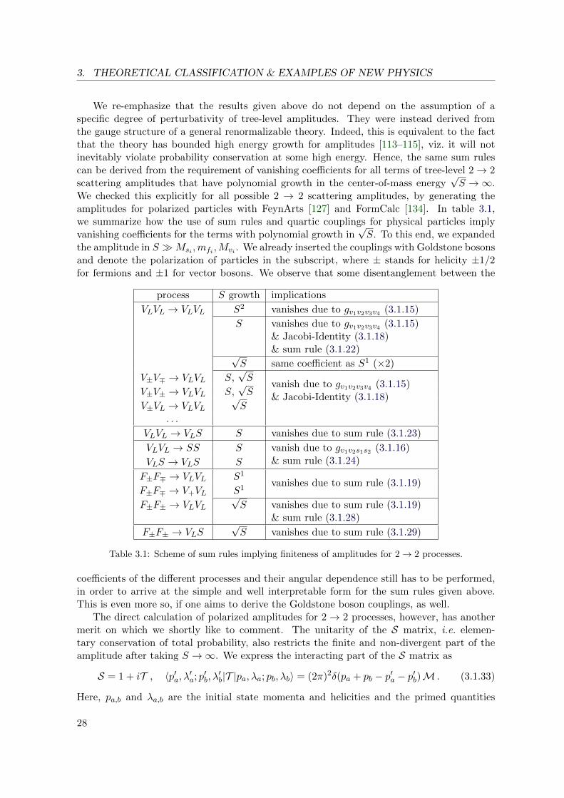
3. THEORETICAL CLASSIFICATION & EXAMPLES OF NEW PHYSICS
We re-emphasize that the results given above do not depend on the assumption of aspecific degree of perturbativity of tree-level amplitudes. They were instead derived fromthe gauge structure of a general renormalizable theory. Indeed, this is equivalent to the factthat the theory has bounded high energy growth for amplitudes [113–115], viz. it will notinevitably violate probability conservation at some high energy. Hence, the same sum rulescan be derived from the requirement of vanishing coefficients for all terms of tree-level 2→ 2scattering amplitudes that have polynomial growth in the center-of-mass energy
√S →∞.
We checked this explicitly for all possible 2 → 2 scattering amplitudes, by generating theamplitudes for polarized particles with FeynArts [127] and FormCalc [134]. In table 3.1,we summarize how the use of sum rules and quartic couplings for physical particles implyvanishing coefficients for the terms with polynomial growth in
√S. To this end, we expanded
the amplitude in S Msi ,mfi ,Mvi . We already inserted the couplings with Goldstone bosonsand denote the polarization of particles in the subscript, where ± stands for helicity ±1/2for fermions and ±1 for vector bosons. We observe that some disentanglement between the
process S growth implications
VLVL → VLVL S2 vanishes due to gv1v2v3v4 (3.1.15)
S vanishes due to gv1v2v3v4 (3.1.15)& Jacobi-Identity (3.1.18)& sum rule (3.1.22)√
S same coefficient as S1 (×2)
V±V∓ → VLVL S,√S
vanish due to gv1v2v3v4 (3.1.15)& Jacobi-Identity (3.1.18)V±V± → VLVL S,
√S
V±VL → VLVL√S
. . .
VLVL → VLS S vanishes due to sum rule (3.1.23)
VLVL → SS S vanish due to gv1v2s1s2 (3.1.16)& sum rule (3.1.24)VLS → VLS S
F±F∓ → VLVL S1
vanishes due to sum rule (3.1.19)F±F∓ → V+VL S1
F±F± → VLVL√S vanishes due to sum rule (3.1.19)
& sum rule (3.1.28)
F±F± → VLS√S vanishes due to sum rule (3.1.29)
Table 3.1: Scheme of sum rules implying finiteness of amplitudes for 2→ 2 processes.
coefficients of the different processes and their angular dependence still has to be performed,in order to arrive at the simple and well interpretable form for the sum rules given above.This is even more so, if one aims to derive the Goldstone boson couplings, as well.
The direct calculation of polarized amplitudes for 2→ 2 processes, however, has anothermerit on which we shortly like to comment. The unitarity of the S matrix, i.e. elemen-tary conservation of total probability, also restricts the finite and non-divergent part of theamplitude after taking S →∞. We express the interacting part of the S matrix as
S = 1 + iT , 〈p′a, λ′a; p′b, λ′b|T |pa, λa; pb, λb〉 = (2π)2δ(pa + pb − p′a − p′b)M . (3.1.33)
Here, pa,b and λa,b are the initial state momenta and helicities and the primed quantities
28

3.1. RELATIONS FOR PERTURBATIVELY UNITARY THEORIES
apply to the final state. The best projections of the angular dependence are achieved bydecomposing the amplitude M in a basis of eigenstates of the total angular momentum withthe helicity formalism of Jacob and Wick [135]. Using the Wigner d-functions dJµµ′ [136] withtotal angular momentum J and the initial and final state helicity differences µ ≡ λa − λb,µ′ ≡ λ′a−λ′b and applying the Wigner-Eckart theorem on the scalar operator T , one can castthe amplitude in the form
M(s, θ) = 32π∑
J
(J + 1
2
)dJµµ′(θ)MJ , (3.1.34)
where θ is the center-of-mass scattering angle and the summation over J runs over all integersstarting from min(µ, µ′). Unitarity of the S matrix implies that eigenvalues of the T operatorhave absolute value smaller than 2, i.e. for the amplitude in the center-of-mass frame
|MJ | ≤√S
2|~pa|S→∞−−−−→ 1 . (3.1.35)
One can improve this bound in the case of elastic scattering starting from T − T † = iT †T ,analogous to the derivation of the optical theorem (e.g. [137]). In the high energy limit itimplies that real and imaginary part of the amplitude lie on a circle with radius 1/2 shiftedalong the imaginary axis [138]
(Im(MJ
)− 1
2
)2+ Re
(MJ
)2 ≤(
12
)2. (3.1.36)
We verified that, in general, interesting bounds can be derived from the s- and p-wavesof the processes VLVL → VLVL, VLVL → VLS, VLVL → SS, VLS → VLS, and the p-waveof F±F∓ → VLVL. Higher partial waves carry decreasing prefactors and therefore becomeless restrictive. The inequalities restrict bilinear sums of couplings with additional factorsup to (mint/mext)
2. They are of interest for light external particles of mass mext, if a veryheavy exchanged particle contributes in the summation with a mass mint mext. Further in-equalities that are linear in the masses are obtained from V±V± → VLVL, V±V∓ → VLVL,F±F± → V+VL, and F±F∓ → VLS. Interesting inequalities may also be derived fromSS → SS and F±F∓ → F∓F±, since they contain a quartic Higgs couplings and scalar–fermion couplings, respectively.
Classically the inequalities have been used to derive upper bounds on the Higgs mass ofthe SM. The most stringent bound follows from the s-wave of WLWL → WLWL, where oneobtains M0 = (GFMh)/(4
√2π) for S Mh [116]. One can extend this beyond a single
channel and bound the largest eigenvalue of the coupled channel matrix for the in- and out-going states
(WLWL,
1√2ZLZL,
1√2hh, ZLh, WLh, WLZL
)[139]. Using the improved bound
(3.1.36) leads to Mh < 710 GeV.7 On the other hand M0 = (GFS)/(16√
2π) follows forthe limit S Mh. This implies that some new physics had to occur in the TeV range, inorder to restore unitary, if the Higgs boson would not exist below this scale. Another classicalapplication was to bound the masses of chiral fermions in the SM [117, 118].
Note that these classical applications of tree-level perturbative unitarity assumed pertur-bativity of the Higgs self-coupling λ = M2
h/(2v2). However, since it grows with the Higgs
7This tree-level estimate for the breakdown of perturbation theory is indeed close to values found bycalculating two-loop corrections [140, 141], and to non-perturbative lattice calculations [138]
29

3. THEORETICAL CLASSIFICATION & EXAMPLES OF NEW PHYSICS
mass, unitarity might also be restored by large loop corrections, signaling the failure of per-turbation theory and the loss of predictivity of the SM [142]. At least, this shows thatbounds derived from tree-level perturbative unitarity can have loopholes. An alternative andpresently more relevant criterion of theoretical bounds on the Higgs mass is precisely derivedfrom the Higgs self-coupling. Finiteness of the running self-coupling up to the Planck scaleleads to Mh . 175 GeV, called the perturbativity bound [138, 143], while positivity impliesMh > 129.4± 1.8 GeV [88], called the stability bound. The present experimental value of theHiggs mass is marginally compatible with the latter bound.
In a similar approach to generic new physics that we take here, the sum rules and inequal-ities from the s- and p-wave of F±F∓ → VLVL have also been derived recently in [122]. Theauthors apply the inequality to interpret unitarization properties in simple W ′ models. Theyfind that an accompanying Z ′ is constrained to have mass below 7–8 TeV if no further scalarscontribute.
We summarize that also the inequalities following from tree-level perturbative unitarityare in general interesting in order to constrain the spectrum of new physics. Our emphasisin this thesis is different, however. We will only resort to the sum rule equations, which wederived in this section. They hold exactly due to gauge invariance. In this way, we will beable to renormalize and simplify the Z-penguin at a generic level in section 4.1.1.
30
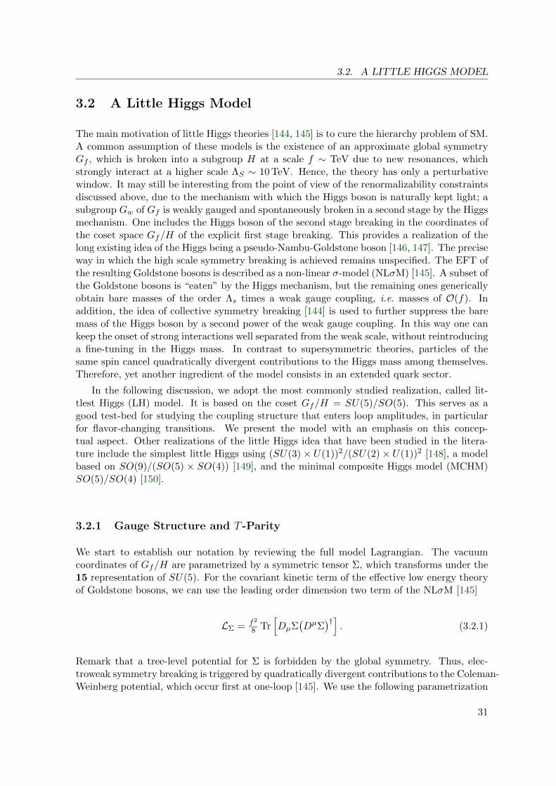
3.2. A LITTLE HIGGS MODEL
3.2 A Little Higgs Model
The main motivation of little Higgs theories [144, 145] is to cure the hierarchy problem of SM.A common assumption of these models is the existence of an approximate global symmetryGf , which is broken into a subgroup H at a scale f ∼ TeV due to new resonances, whichstrongly interact at a higher scale ΛS ∼ 10 TeV. Hence, the theory has only a perturbativewindow. It may still be interesting from the point of view of the renormalizability constraintsdiscussed above, due to the mechanism with which the Higgs boson is naturally kept light; asubgroup Gw of Gf is weakly gauged and spontaneously broken in a second stage by the Higgsmechanism. One includes the Higgs boson of the second stage breaking in the coordinates ofthe coset space Gf/H of the explicit first stage breaking. This provides a realization of thelong existing idea of the Higgs being a pseudo-Nambu-Goldstone boson [146, 147]. The preciseway in which the high scale symmetry breaking is achieved remains unspecified. The EFT ofthe resulting Goldstone bosons is described as a non-linear σ-model (NLσM) [145]. A subset ofthe Goldstone bosons is “eaten” by the Higgs mechanism, but the remaining ones genericallyobtain bare masses of the order Λs times a weak gauge coupling, i.e. masses of O(f). Inaddition, the idea of collective symmetry breaking [144] is used to further suppress the baremass of the Higgs boson by a second power of the weak gauge coupling. In this way one cankeep the onset of strong interactions well separated from the weak scale, without reintroducinga fine-tuning in the Higgs mass. In contrast to supersymmetric theories, particles of thesame spin cancel quadratically divergent contributions to the Higgs mass among themselves.Therefore, yet another ingredient of the model consists in an extended quark sector.
In the following discussion, we adopt the most commonly studied realization, called lit-tlest Higgs (LH) model. It is based on the coset Gf/H = SU(5)/SO(5). This serves as agood test-bed for studying the coupling structure that enters loop amplitudes, in particularfor flavor-changing transitions. We present the model with an emphasis on this concep-tual aspect. Other realizations of the little Higgs idea that have been studied in the litera-ture include the simplest little Higgs using (SU(3)× U(1))2/(SU(2)× U(1))2 [148], a modelbased on SO(9)/(SO(5) × SO(4)) [149], and the minimal composite Higgs model (MCHM)SO(5)/SO(4) [150].
3.2.1 Gauge Structure and T -Parity
We start to establish our notation by reviewing the full model Lagrangian. The vacuumcoordinates of Gf/H are parametrized by a symmetric tensor Σ, which transforms under the15 representation of SU(5). For the covariant kinetic term of the effective low energy theoryof Goldstone bosons, we can use the leading order dimension two term of the NLσM [145]
LΣ = f2
8 Tr[DµΣ
(DµΣ
)†]. (3.2.1)
Remark that a tree-level potential for Σ is forbidden by the global symmetry. Thus, elec-troweak symmetry breaking is triggered by quadratically divergent contributions to the Coleman-Weinberg potential, which occur first at one-loop [145]. We use the following parametrization
31

3. THEORETICAL CLASSIFICATION & EXAMPLES OF NEW PHYSICS
of the matrix Π of the 14 Goldstone bosons
Σ = eiΠ/fΣ0eiΠT/f = e2iΠ/fΣ0 , Σ0 =
0 0 12
0 1 012 0 0
,
Π = χaXa =
Γ + η 1√20
Φ −i∆Φ† −η
√45 ΦT
i∆∗ Φ∗ Γ∗ + η 1√20
,
(3.2.2)
and denote the possible VEVs of the neutral scalars h and φ0 as v and v′. The componentsof the doublet Φ, triplet ∆, and Γ are given by8
Γ = −ω0 σ3
2 − iω+ σ+√2
+ iω− σ−√2,
Φ =(
1√2π+ , 1
2
(v + h+ iπ0
))T,
∆ =
(φ++ 1√
2φ+
1√2φ+ 1√
2
(v′ + φ0 + iφP
)). (3.2.3)
The broken generators τa ∈ SU(5) can be identified as being odd under the automorphism
τaT−→ −Σ0(τa)TΣ0 , (3.2.4)
while the unbroken generators are even. The image of the Goldstone boson matrix under thisautomorphism is given by
ΣT−→ Σ = Σ0ΩΣ†ΩΣ0 , Ω ≡ diag(1, 1,−1, 1, 1) . (3.2.5)
Remark that the VEV of Σ can be expressed in short and exact form as
〈Σ〉 =
0 0 0 1 0
0 12α+ v′
v βi√2
(β − v′
v α)
0 1 + α(
12 +
(v′
v
)2)
0 i√2
(β − v′
v α)
1 + α 0 i√2
(β + v′
v α)
1 0 0 0 0
0 1 + α(
12 +
(v′
v
)2) i√2
(β + v′
v α)
0 12α− v′
v β
,
with α ≡cos(
v√2f
)− 1
1 +(v′
v
)2 , β ≡sin(
v√2f
)√
1 +(v′
v
)2 .
(3.2.6)
It is suitable to choose Gw = (SU(2) × U(1))1 × (SU(2) × U(1))2 as the weakly gaugedsubgroup. Since it does not entirely lie in the remnant SO(5), the high scale breaking G→ Halso breaks Gw and the additional gauge bosons obtain TeV-scale masses.
global: SU(5)〈Σ〉−−−→ SO(5)
∪ (g1,2) ∪ (g = sg1 = cg2)
local:[SU(2)× U(1)
]2 〈Σ〉−−−→[SU(2)× U(1)
]diag
8Conventionally, the Goldstone bosons in Φ are denoted by the symbols π, to express the analogy to thepions from the chiral symmetry of QCD. In this context, they correspond to the usual Goldstone bosons of theSM Higgs doublet, which we called ϕ in (2.2.6). In particular, they do not obtain mass by symmetry breaking;instead h becomes the pseudo Goldstone-boson.
32

3.2. A LITTLE HIGGS MODEL
The interesting aspect of this symmetry breaking pattern is that each SU(2)×U(1) ⊂ SU(5)has a full global SU(3) symmetry in its coset. Each of the two SU(3) symmetries protectsthe one-loop scalar potential, which we discuss below, from developing a coefficient for theHiggs mass Mh. Thus, both couplings g1 and g2 have to be present in a diagram in orderto generate a Higgs mass term, which is then naturally light compared to the cutoff scaleΛs. This is referred to as collective symmetry breaking [144]. The charges and the covariantderivative of Σ in Gw are given by
Qi1 =
(σi
2 00 03
), Qi2 =
(03 0
0 −σi∗
2
),
Y1 = 110 diag(3, 3,−2,−2,−2) , Y2 = 1
10 diag(2, 2, 2,−3,−3) ,
(3.2.7)
DµΣ = ∂µΣ− iV(Σ) , V(Σ) = gjWaj (QajΣ + Σ(Qaj )
T )− g′jBj(YjΣ + ΣYj) . (3.2.8)
The given direction9 of Gw in Gf ensures that the diagonal subgroup of Gw is unbroken byΣ0 and can therefore represent the SM-like SU(2)L×U(1)Y . The appropriate rotation fulfillsgjWjQj = g(WQ+W ′Q′) and reads 10
W ′ = cW1 − sW2 , W = sW1 + cW2 ,
Q = Q1 +Q2 , Q′ = csQ1 − s
cQ2 , g = sg1 = cg2(3.2.9)
An analogous rotation is applied for Bj , g′jYj , and angles θ′ instead of Wj , gjQj , and θ. The
trigonometric functions are denoted by c(′) = cos(θ(′)), s(′) = sin(θ(′)), and t(′) = tan(θ(′)),and analogous for further angles, which are defined below.
In the general setup discussed above, the scale f has been found to be pushed to valuesbeyond 4 TeV, because of large contributions to electroweak precision observables [153–155].The fact that the corresponding dimension six operators are sourced by tree-level exchanges ofnew particles, suggests an obvious way to alleviate the bounds. A simple Z2 symmetry calledT -parity [156], under which only SM-like fields are even, can circumvent the bounds. Thisis simply done by promoting the automorphism (3.2.4) to a fundamental symmetry, whichinterchanges the two SU(2)×U(1) gauge groups. Thus, it acts on gauge fields as T : A1 ↔ A2
where Ai = W ai Q
a or BiY . We furthermore define the action on scalars as T : Π → −ΩΠΩ.This obviously renders all scalars T -odd except those contained in the doublet Φ. Remarkthat the invariance of the Lagrangian together with T -parity implies equal gauge couplings
g(′)1 = g
(′)2 =
√2 g(′). We continue to present the general setup for gauge bosons and comment
on an issue concerning the gauge fixing procedure, necessary for the quantization of the theory.The T -parity symmetric case (LHT model) can be obtained by the specific choice of someof the parameters. We will only refer to the latter for the calculation of the flavor-changingZ-transitions in chapter 3.1, since the T -symmetric case turns out to be phenomenologicalmore interesting, and has a richer fermion sector.
As stated above, the Coleman-Weinberg-potential triggers electroweak symmetry breakingat one-loop order. It was recognized in [151] that we obtain essentially three new parameters.
Two of them are the mass Mh for the Higgs boson h and the degenerate masses M2φ = 2f
2
v2M2h
9One assumes the dynamics of the unknown UV completion to choose this direction of Gw relative to Σ0.10We define W ′ and B′ with an additional sign compared to most of the literature on the LH without T -
Parity [151, 152]. This sign convention is compatible with all the literature on the LH with T -Parity. In orderto agree with most of the literature, we also use a reversed sign for the coupling g′ compared to section 2.2.
33
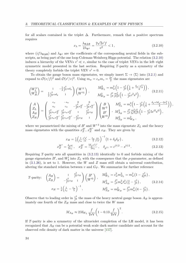
3. THEORETICAL CLASSIFICATION & EXAMPLES OF NEW PHYSICS
for all scalars contained in the triplet ∆. Furthermore, remark that a positive spectrumrequires
xλ =λΦ∆Φ
2λΦ4
=2√
2v′fv2
< 1 , (3.2.10)
where (ifλΦ∆Φ) and λΦ4 are the coefficients of the corresponding neutral fields in the sub-scripts, as being part of the one loop Coleman-Weinberg Higgs potential. The relation (3.2.10)induces a hierarchy of the VEVs v′ v, similar to the case of triplet VEVs in the left–rightsymmetric model presented in the last section. Requiring T -parity as a symmetry of thetheory completely forbids the triplet VEV v′ = 0.
To obtain the gauge boson mass eigenstates, we simply insert Σ → 〈Σ〉 into (3.2.1) andexpand to O(v/f)2 and O(v′/v)2. Using mw = cwmz = gv
2 the mass eigenstates are
(W±LW±H
)=
(1 −1
2v2
f2 csδg
12v2
f2 csδg 1
)(W±
W ′±
),
M2WL
= m2w
(1− v2
f2
(16 +
δg−x2λ
4
)),
M2WH
= f2
v2m2w
c2s2
(1− v2
f2 c2s2),
(3.2.11)
AZLAHZH
=
cw −sw 0 0
sw cw − v2
f2 xB′Z − v
2
f2 xW ′Z
v2
f2 swxB′Z
v2
f2 cwxB′Z 1
v2
f2 xH
v2
f2 swxW ′Z
v2
f2 cwxW ′Z − v
2
f2 xH 1
BW 3
B′
W ′3
,
M2ZL
= m2z
(1− v2
f2
(16 +
δg+5δg′−2x2λ
4
)),
M2AH
= f2
v2m2wt
2w
5c′2s′2
(1− v2
f2 5c′2s′2),
M2ZH
= m2WH
,
where we parametrized the mixing of B′ and W ′ 3 into the mass eigenstate ZL and the heavymass eigenstates with the quantities xB
′Z , xW
′Z and xH . They are given by
xH = 14
(1tw
c′s′
cs − tw5
csc′s′
)−1(1 + δgδg′
), (3.2.12)
xW′
Z =δgsc2cw
, xB′
Z =5δg′s
′c′
2sw, δg(′) = c(′) 2 − s(′) 2 . (3.2.13)
Requiring T -parity sets all quantities in (3.2.13) identically to 0 and forbids mixing of thegauge eigenstates B′, and W ′3 into ZL with the consequence that the ρ-parameter, as definedin (3.1.26), is set to 1. However, the W and Z mass still obtain a universal contribution,altering the standard relation between v and GF . We summarize for further reference
T -parity:
(AHZH
)=
(1
v2
f2 xH
− v2
f2 xH 1
)(B′
W ′3
),
xH = 14
(1tw− tw
5
)−1,
M2WL
= c2wm
2ZL
= m2w
(1− v2
6f2
),
M2AH
= f2
v2m2wt
2w
(45 − v2
f2
),
M2ZH
= m2WH
= f2
v2m2w
(4− v2
f2
).
(3.2.14)
Observe that to leading order in v2
f2 the mass of the heavy neutral gauge boson AH is approx-imately one fourth of the ZH mass and close to twice the W mass
MAH ≈ 2MWL
f
TeV
(1− 0.13
f
TeV
)2
. (3.2.15)
If T -parity is also a symmetry of the ultraviolet completion of the LH model, it has beenrecognized that AH can be a potential weak scale dark matter candidate and account for theobserved relic density of dark matter in the universe [157].
34

3.2. A LITTLE HIGGS MODEL
Up to now, we brought the bosonic mass terms into canonical form. We also need toaccount for standard kinetic terms of the scalars, which are a priori spoiled in the basis of(3.2.2) because of the NLσM, and consider the mixing terms of scalars with gauge bosonsarising from LΣ of (3.2.1). The former is achieved by a hermitian redefinition of the scalars.This is due to the fact that, e.g. in the neutral sector, the kinetic terms can be cast into theform
LΣ ⊃1
2
∑
φa
∂µφa(δab + v2
f2Hab
)∂µφb , (φa = h, φ0, φP , π0, η, ω0) , (3.2.16)
with Hab forming a hermitian matrix. Therefore, we simply redefine φ′a =(δab + v2
2f2Hab
)φb.
Thereafter, we are still allowed to make a unitary redefinition of the scalar fields withoutspoiling the canonical kinetic terms. We can finally render the terms
LΣ ⊃ −f2
4 Im Tr[(∂µΣ
)V(Σ)†
](3.2.17)
canonical in the mass basis, i.e. of the form −σaMV a(∂µV amµ)φam, where the subscript m
denotes fields in the mass basis. A treatment of the charged scalar sector is analogous. Thenecessary redefinition is unitary at O(v2/f2, v′2/v2, v′/f) and included in appendix A.2. Weremark, that we found the redefinition to be non-unitary starting at O(vv′/f2) = O(v3/f3).This indicates the necessity of a non-linear gauge fixing procedure at subleading order inthe expansion in v/f . However, considering the divergence structure of ∆F = 1 amplitudesdiscussed in chapter 3.1, it is important to see that the leading contributions can be calculatedreliably in the standard quantization approach.
The bosonic Lagrangian is completed by standard covariant kinetic terms LV of the lin-early realized gauge bosons of Gw. We give LV for completeness in (A.2.1).
3.2.2 Fermion Sector
Since little Higgs models are constructed as a solution to the hierarchy problem, one alsoaddresses the one-loop contributions to the Higgs boson mass from the top-Yukawa coupling.This is done via a contribution of the same order y2
tΛ2S/(16π2) ∼ f2 originating from an
additional vector-like heavy fermion. We will discuss the LHT model in the following. Itturns out that the setup without T -parity requires only one new fermion, which also appearsin the model with T -parity and has similar couplings.
As an additional obstacle in the LHT model, one has to assure that the SM fermionsare introduced as T -even states. This is achieved by introducing two doublets ψ1,2 thateach transform linearly under one of the SU(2) groups in Gw. Only the remaining T -oddlinear combination shall get a mass of order f , which is achieved by introducing a full SO(5)multiplet of T -odd mirror fermions Ψ′ [158]. To this end, a non-linear realization of SU(5)avoids the introduction of yet another copy of mirror fermions, and completeness of themultiplet again protects the Higgs mass from a potential two-loop quartic divergence [159].
We first summarize the relevant fermion content of the model. It has been realized in [160]that in order to accommodate the hypercharge of the Standard Model fermions, one has toadd two U(1) factors to the original setup. For each of these U(1) factors only the diagonalsubgroup with one of the U(1) factors contained in Gw is gauged. Here we summarize onlythe resulting charges for the gauged groups in table 3.2.
35

3. THEORETICAL CLASSIFICATION & EXAMPLES OF NEW PHYSICS
q1,i uci dci qHR,i t′1 t′c1 l1,i eci lHR,iSU(2)1×2 (2, 1) (1, 1) (1, 1) (1, 1) (1, 1) (2, 1) (1, 1)
Y1 1/30 1/3 −1/6 1/3 8/15 8/15 −3/10 −1/2 0Y2 2/15 1/3 −1/6 1/3 2/15 2/15 −1/5 −1/2 0
T −q2,i + + − −t′2 −t′c2 −l2,i + −
Table 3.2: Charges for the full fermion sector of the LHT model. In the last line, we giveeither T eigenvalues or the definition for the fields q2,i, t
′2, t′c2 , l2,i as the T -parity image of
the corresponding fields.
T -parity eigenstates for the fermions are given by
qL,i = 1√2
(q1,i − q2,i
), qHL,i = 1√
2
(q1,i + q2,i
), t′± = 1√
2
(t′1 ∓ t′2
)(3.2.18)
and analogous linear combinations for leptons ln,i and the right-handed top partner fermionst′cn . Here qn,i = (un,i, dn,i)
T denotes two fundamental quark doublets. The T -even top partnert′+ now has the same quantum numbers like the SM-like up-type quarks uL,i and may mixwith them. To write down the Lagrangian, we embed the fermion content into incompleterepresentations of SU(5)
Ψ1,i =
ψ1,i
00
, Ψ2,i =
00ψ2,i
, Ψ′i =
ψ′iχ′iψ′i
, (3.2.19)
where ψn,i = −iσ2qn,i and ψ′i = −iσ2qHR,i. ψ′ and χ′ are assumed to obtain very large Dirac
masses from couplings to additional fermions and can be safely decoupled from the theory[157]. Using ξ = eiΠ/f the mirror mass terms are given by
Lmirror = fκij(Ψ2,iξ + Ψ1,iΣ0Ωξ†Ω
)Ψ′j . (3.2.20)
After a singular value decomposition of κ and rotation of the mirror fermions f = u, d
κ = VH diag(mqH,i√
2f
)U †H , fHL,i = (VH)ijf
(m)HL,j , fHR,i = (UH)ijf
(m)HR,j , (3.2.21)
we obtain masses mdH,i = mq
H,i and muH,i = mq
H,i
(1 − v2
8f2
). The upper index (m) in (3.2.21)
stands for mass eigenstates. We will skip the index in the following and work with masseigenstates only. Mirror masses for leptons can be written down in full analogy.
For the Yukawa interactions of the T -even fermions, it is convenient to define
Qn,i ≡ Ψn,i + δn,3 (0, i t′n, 0)T , Ψ′n,i ≡ (qn,i, 0, 0)T , X = (Σ33)−1/4 . (3.2.22)
Gauge invariant Yukawa interactions and a T -even Dirac mass term for t′n are given by
LY,u = i2√
2f (λU )ij
3∑
i,j,k=1
5∑
x,y=4
εabc εxy
[(Q2,iΣ0
)a
Σbx Σcy −(Q1,i
)a
Σbx Σcy
]ucj
− fλ+(t′1t′c1 + t′2t
′c2 ) + h.c. , (3.2.23)
LY,d = i2√
2f (λD)ij
2∑
a,b=1
5∑
x,y,z=3
εab εxyz
[(Ψ′2,i
)x
Σay ΣbzX −(Ψ′1,iΣ0
)x
Σay Σbz X]dcj + h.c.
36

3.2. A LITTLE HIGGS MODEL
The Lagrangian implements the idea of collective symmetry breaking. This is due to thefact that Qn,i is an incomplete representation of the subgroup SU(3)i in SU(5), which is leftinvariant when gi = 0, for i = 1 and 2 respectively.11 Remark that for this reason t− doesnot couple to the Higgs boson directly and does not participate in the processes discussed insection 4.3.
We start the diagonalization of the mass terms by going into a basis where λD is diagonalvia two unitary redefinitions in the down sector. t′− does not mix with other fermions. Wedenote its mass eigenstate with T− = t′−. Its mass is given by mT− = fλ+. The remainingmass matrix for the up-quarks U = (u, c, t, t′+) is given by
LY,u ⊃ −ULMU UR + h.c. , MU = v
(λU(1− v2
3f2
)0
(λU )3n
(1− v2
2f2
)λ+
fv
), (3.2.24)
where the third row elements of the 3× 3 matrix λU are repeated in the fourth row of MU .In all of the existing literature we are aware of, the diagonalization of this matrix assumesvanishing λ31, λ32 and only applies rotations in the t − t′+ sub-block. Explicit treatmentsare given e.g. in [151, 163–168]. The first assumption is justified, since we know the generalsolution can be written as
V†uMUUu =
(V † 00 1
)diag(mu,mc,mt,mT+) , (3.2.25)
where V is a CKM-like unitary 3× 3 matrix, and Vu, Uu are perturbations around the unitmatrix. Consequently, (λU )31, (λU )32 are chirally suppressed. However, the t − t′+ rotationproduces off-diagonal terms in the (1, 4) and (2, 4) entries on the right-hand side of (3.2.25),which are only suppressed by the square of the Cabibbo-angle, λ2, and are not chirallysuppressed. While it is still reasonable from a phenomenological point of view to neglectthose terms, this assumptions is usually not stated explicitly. We take u, c − T+ mixingsinto account, in order to keep the coupling structure most general. This is useful for testingthe generic result on flavor-changing Z transitions in chapter 3.1. We will see below thatterms implied by these new rotations can be summarized in a sensible vertex definition ofthe CKM matrix. To this end, we derived the exact decomposition of (3.2.25) and neglectedchirally suppressed mu,c/mt only afterwards. The intermediate step of this calculation arecumbersome but result only in two simple, additional, elementary rotations for the left-handedup-quarks. The mass eigenstates of the up-quarks are finally given by
UR = Uu (u(m), c(m), t(m), T+)TR , UL = Vu
(V † 00 1
)(u(m), c(m), t(m), T+)TL , (3.2.26)
with the unitary matrices
Uu =
12 0
0cR sR−sR cR
, Vu =
12 0
0cL sL−sL cL
1 0 0 00 ccL 0 scL0 0 1 00 −scL 0 ccL
cuL 0 suL0 12 0−suL 0 cuL
.
11For the LH model without T -parity, the authors of [161, 162] showed that the assumption of a commonSU(3) symmetric Yukawa coupling y1 for the components in Qn is unstable against radiative corrections. Thisimplies a two-loop quadratic divergence to the Higgs mass, which is estimated to be of the same order asthe logarithmically divergent one-loop contribution, and requires a certain amount of hidden fine-tuning or anintricate UV completion.
37

3. THEORETICAL CLASSIFICATION & EXAMPLES OF NEW PHYSICS
We choose phases for the entries of V in a non-standard convention, with positive entries in
the third row. This renders the given angles c(u,c)L,R free of phases and particularly simple
sR =√xL
(1− v2
f2
(12 −
xLV 2
33
)(1− xL)
), cR =
√1− xL
(1 + v2
f2
(12 −
xLV 2
33
)xL
)),
sL = vf xL
(1 + d2
v2
f2
), cL = 1− v2
f2
x2L2 ,
scL = vf xL
(1 + v2
f2
(d2 +
x2L2
))V32
V33, ccL = 1− v2
f2
x2L2V 2
32
V 233
,
suL = vf xL
(1 + v2
f2
(d2 +
x2L2
1−V 231
V 233
))V31
V33, cuL = 1− v2
f2
x2L2V 2
31
V 233
,
(3.2.27)
d2 = −56 + xL − x2
L2 + xL(1−xL)
V 233
, (3.2.28)
where xL = λ2U,33/(λ
2U,33 + λ2
+), the unitary CKM entries Vij , and the SM quark masses arenow used as the model input parameters. The value of xL is constrained by electroweak pre-cision data [169], but the exact constraint strongly depends on the realization and parametersof the T -odd sector and possible UV dependent terms. Remark that our definition of V isdifferent from the usual definition in the literature in two ways. There, higher orders in theCabibbo angle are implicitly neglected, which amounts to setting suL = scL = 0. Furthermore,Vu is effectively defined as being commuted with the unitary CKM when compared to ourdefinition. We checked that the redefinition Vij → cL(Vliterature)ij for (i = 3) 6= (j = 3)reproduces the results for charged currents at O
(v2/f2 · λ0
). As anticipated above, we define
the CKM matrix via the W -vertex to light fermions
W+
dj
ui
= ig√2Vij , Vij ≡ Vij −
v2
f2
x2L
2V 233
(Vij V3j + 2
j−1∑
k=1
VikV3k
)V3j . (3.2.29)
The usage of V , instead of V , in the Feynman rules, which we enlist in appendix A.2, encodesall higher order corrections in the Cabibbo angle as compared to the literature. Furthermore,it simplifies the expressions derived in section 3.1 significantly. We note in passing, that the3× 3 CKM matrix V is non-unitary. This is expected if the sum-rule (3.1.19) holds, like wediscussed it in the text below this equation. The only additional contribution to this sumrule is given by a T+ quark exchange, using the Feynman rules of appendix A.2 we expect
(V †V
)ij− δij =
v2
f2
g2x2L
2V 233
V3iV3j , (3.2.30)
if the sum rule holds. Indeed, this is the case as we can easily check from the definition(3.2.29) and the unitarity of V . From the O(v2/f2 · λ6) suppression in (3.2.30), it is alreadyclear that non-unitarity of the first column, ∆non
col1 ≡ 1−∑i |V1i|2 < 0, is tiny and way belowthe observable limits, which are of the order of 10−2 [170]. Non-unitarity of the first row isbetter constrained by approximately one order of magnitude. However, in the LHT model,the sum rules imply that in a unitarized version of the model
(V V †
)ij− δij ∝ δi3δj3, i.e. no
first row non-unitarity would be present at all, while the definition (3.2.29) again gives a result∆non
row1 = O(v2/f2 · λ6). Consequently, non-unitarity is unobservable in all cases. However, afull analysis of non-unitarity aspects would furthermore require the calculation of corrections
38

3.2. A LITTLE HIGGS MODEL
to charged current mediated processes that enter the extraction of the CKM matrix elementsfrom experiment and appear at one loop in the model at hand. The mass eigenvalues of theheavy top-quark partners mT± are fixed by the relations
m2t
m2T−
=v2
f2
xLV 2
33
,m2T+
m2T−
(1− xL) = 1 +v2
f2xL
(xLV 2
33
− 1
). (3.2.31)
Since 0 < xL ≤ 1, we see that the minimal mass for the T -even top partner is given by
mT+ ≥4f
vmt V33 ≈ 2.8 f . (3.2.32)
Yukawa interactions for leptons can be written down analogously to LY,d. We refrain fromintroducing right-handed neutrinos.
Kinetic terms for the linearly transforming fermion multiplets are straightforward to write
down [157, 171]. Remark that Ψ′2 transforms as a 5 and g(′)1 = g
(′)2 =
√2 g(′), such that we
obtain
LF,lin =∑
i=1,2
Ψ′ii /D(i)
Ψ′i +∑
f=uc,dc,t′i,t′ci
f i /Df ,
D(1)µ = Dµ − i
√2g(Qa1W
a1µ +Qa2W
a2µ
),
D(2)µ = Dµ + i
√2g((Qa1)TW a
1µ + (Qa2)TW a2µ
),
Dµ = ∂µ + i√
2g′(Y1B1µ + Y2B2µ
). (3.2.33)
Furthermore, we also need a kinetic term for the right-handed mirror fermions. It is con-structed by following the approach of Callan, Coleman, Wess and Zumino [172, 173]. Anexplicit construction of the necessary Maurer-Cartan one form was first given in [158, 159]
LF,mir = 12Ψ′[ξ†i /D(1)
ξ + ξΣ0i /D(1) ∗
Σ0ξ†]Ψ′ . (3.2.34)
The hypercharge in /D(1)
must be adapted to account for the insertion of ξ, i.e. explicitly
Y = Y(ξΨ′)i = Y
(Σ)i + Y
(Ψ′)i . It is useful to note that in terms of T -parity eigenstates
Σ0 /D(1) ∗
Σ0 = ∂µ − ig(QaW aµ −Q′aW ′aµ ) + ig′(Y Bµ − Y ′B′µ) (3.2.35)
Remark that one has to take special care when deriving the interactions of mirror fermionsfrom (3.2.34), since their couplings to ZL and WL are not vector-like at O(v2/f2) afterelectroweak symmetry breaking [160]. This has implications on perturbativity of the theoryand the calculations performed in chapter 3.1. Furthermore, heavy gauge bosons mediatecurrents between a SM fermion and a mirror fermion. Those interaction are all proportionalto a combination of heavy and light mixing matrices, for which it is useful to introduceabbreviations
VHd ≡ V †H , VHu ≡ VHd V † . (3.2.36)
The matrix VH was defined in (3.2.21). It introduces three new mixing angles and threeCP -violating phases [174]. In the context of flavor observables they allow for interestingdepartures from the minimally flavor violating patterns. Since we are only interested in thecoupling structure of the model and do not study the precise numerical consequences of themodel, we end the discussion at this point and refer to the given references for further details.
39

3. THEORETICAL CLASSIFICATION & EXAMPLES OF NEW PHYSICS
3.3 Randall-Sundrum Models
As a last example of physics beyond the SM we present models with a warped extra dimension.They belong to the class of theories for which non-perturbativity at a given new energy scale,is directly implied by construction. The models become strongly interacting due to loweringthe effective scale of gravity for heavy fermions and, most prominently, for the Higgs boson.However, they do not aim to reduce the little hierarchy problem in contrast to the little Higgsmodels presented in the last section.
The first scenario of this type was first proposed by Randall and Sundrum [175]. Itprovides a natural explanation for the absence of the gauge-hierarchy problem, and also avery compelling theory of the hierarchies in the flavor sector. Therefore, such models areespecially interesting from a precision physics perspective as they receive relevant constraintsfrom electroweak precision physics, flavor-changing decays and most recently also from Higgsproduction and decays. In combination with the rather small number of free parameters thiscreates a good prospect for their falsifiability.
We give a short introduction into the necessary geometric structure of the extra dimensionand discuss a minimal realization of the Randall-Sundrum (RS) model. As for the theoriesdiscussed in the previous section, we also present an extension of the RS model that ac-counts for the strongest electroweak precision constraints by implementing an enlarged gaugesymmetry sector and a specific fermion embedding, the custodial RS model.
3.3.1 Basic Geometry of the Setup
Quantum field theories with extra dimensions offer an interesting candidate as a fundamentaltheory since they provide a framework that naturally connects the electroweak scale with ahigher fundamental scale. The geometry of the extra dimension is explicitly adapted to servethis purpose. Length scales rc orthogonal to our usual 3+1 space-time are usually compactifiedand resolvable with energies not too far above the electroweak scale 1/rc ∼ ΛIR & Mweak.The higher scale ΛUV can be implemented in various ways and is mostly used to establish ageometric connection to gravity. The first viable scenarios with large and flat extra dimensionswere proposed in the late ’90s by Arkani-Hamed, Dimopoulos and Dvali (ADD) [176] whichcan be regarded as the root of this branch of model building. In these theories it is illustrativeto compare Newton’s law at distances much smaller than rc which has a fundamental Planck
scale M(4+n)Pl , with Newton’s law relevant to a macroscopic observer at distances much larger
than rc. The latter shows an effective Planck scale(M
(4,eff)PL
)2 ≈(M
(4+n)PL
)2+nrnc , when
using n extra dimensions of equal size. For large enough rc or n we obtain a potentiallylarge separation between the fundamental and the effective scale. Colloquially one says thatthe propagation of gravity in the bulk of the extra dimensions dilutes its force compared toother forces whose quantum fluctuations can be localized to a specific position in the extradimension. As in every model, the fundamental Planck scale also serves as the UV cutoff ofthe theory, since one expects the onset of a quantum theory of gravity at this scale. Choosing
a low scale M(4+n)Pl = ΛIR ∼ 1 TeV and the effective scale M
(4,eff)Pl = MPL ∼ 1016 TeV gives a
natural explanation for the absence of the gauge-hierarchy problem in this effective theory dueto gravity. This is analogous to the onset of QCD-like strong interaction in composite Higgsmodels. However, to obtain the numerical values given above, n < 3 dimensions are excludedby direct measurements of the inverse square law [177] and astrophysical measurements ofthe release of gravitational binding energy in type-II supernovae [178]. The latter takes place
40

3.3. RANDALL-SUNDRUM MODELS
through nucleon-nucleon scattering processes, where the light Kaluza Klein (KK)-gravitonstates are produced in the final state. KK states are the Fourier-modes of a quantum fieldthat extends into a compactified extra dimension, like the graviton does in the ADD model.Besides the strong direct bounds, the ADD model has the theoretical drawback that theseparation of Planck and electroweak scale is achieved only by the introduction of yet anotherscale parameter rc without explaining its size. One way to overcome this was proposed byRandall and Sundrum [175] through the use of a non-trivial geometry in a 5d anti-de Sitterspace AdS5. For their setup a single extra dimension is sufficient, given the non-factorizablemetric
ds2 = e−2σ(φ) ηµν dxµdxν − r2 dφ2 ; σ(φ) = kr|φ| . (3.3.1)
Here, xµ denote the coordinates on the 4d hyper-surfaces of constant φ with metric ηµν =diag(1,−1,−1,−1). Length and energy scales are modified by the exponential warp factorσ(φ) depending on the extra coordinate φ ∈ [−π, π]. For the localization of fields and tomake the geometry a solution to 5d Einstein equations, is reasonable to introduce topologicaldefects, so-called branes, in the form of an orbifold.12 Here, the S1/Z2 orbifold compactifi-cation leaves two 3-branes that are located at the orbifold fixed points at φ = 0 (UV brane)and φ = π (IR brane). The curvature parameter k and the inverse radius r−1 of the extradimension are assumed to be of the size of the only fundamental mass parameter MPl. Asmentioned above the fundamental energy scale is position-dependent and in fact MPl e
−σ(φ)
sets the effective Planck scale at a given point along the extra dimension. It serves as a natu-ral UV cutoff, since quantum gravity becomes relevant above this scale. Higher-dimensionalspaces with warp factors arise naturally in flux compactifications of string theory [181–184],which could provide a UV completion of this effective model. Like in the ADD model, oneassumes that the effective cutoff scale on the IR brane ΛTeV = MPl e
−σ(π) ≡ MPl ε is inroughly around 20 TeV in order to solve the (big) hierarchy problem. In contrast to theADD model the exponential hierarchy of energy scales is generated by the AdS5 backgrounditself. This requires L ≡ krπ = − ln ε ≈ 34 to be only moderately large, leaving a littlehierarchy problem: The fact that the Higgs mass is two orders of magnitude smaller thanthe cutoff scale, is not addressed in the minimal RS framework. The warped curvature scale,MKK ≡ ke−σ(π) = kε, is assumed to lie somewhat lower, in the range of a few TeV. Thisallows for predictive phenomenology since MKK sets the mass scale for the low-lying KKexcitations of the SM fields. The first KK photon and gluon states in fact obtain masses of2.45MKK, the first KK graviton a mass of 3.83MKK, and fermion masses are in a similarrange [185]. Another conceptual difference to the ADD model is that the effective Planck
scale(M
(4,eff)Pl
)2=(M
(5)Pl
)3(1 − e−2πkr
)/k ∼ M2
Pl is of the same size as all the introducedfundamental mass parameters [175].
It will be convenient to introduce a conformal coordinate for the extra dimension. Here,we use it in the way of reference [186] with mass dimension zero as t = ε eσ(φ) as this rendersthe results especially compact: t equals ε on the UV brane and 1 on the IR brane. Integralsover the orbifold are obtained using
π∫
−π
dφ→ 2π
L
1∫
ε
dt
t,
π∫
−π
dφ eσ(φ) → 2π
Lε
1∫
ε
dt . (3.3.2)
12Another possibility of confining fields to regions of finite width (“fat branes”) uses domain wall solutionsof additional scalar fields [179] and has been used e.g. in [180] to separate the positions of fermions in largeextra dimensions. The branes in the RS model are not of this kind, so we will not further elaborate on this.
41

3. THEORETICAL CLASSIFICATION & EXAMPLES OF NEW PHYSICS
The form z = t/MKK includes the appropriate mass scale to write the metric conformally[187]
ds2 =
(R
z
)2(ηµν dx
µdxν − dz2), (3.3.3)
and is also often used in the literature. To facilitate comparison we note that z ∈ [R,R′], whereR = 1/k and R′ = 1/MKK denote the positions of the UV and IR branes, and L = ln(R′/R).
It has been noted by Goldberger and Wise [188] that the geometric setup of the givendistance between the two branes described above can be stabilized. The radion is the scalarquantum fluctuation along the coordinate φ. Its potential has to be modeled such that theradion VEV determines the size of the extra dimension L. Additionally, the radion mustbe massive, which is necessary because of the equivalence principle [175]. All this can beachieved with the introduction of an additional scalar field and only moderate fine-tuningin its corresponding coupling parameters. Remark that in principle one may introduce amixing parameter for the Higgs boson with the radion. For definiteness we will assume it tobe negligible, or equivalently assume a large mass of the radion. We refer to [189–191] for acloser discussion.
We close the discussion of the geometry with a short comment on the actual size of L.From a purely phenomenological point of view, it is possible to lower the UV cutoff fromthe Planck scale to a value only few orders of magnitude above the TeV scale. This lessambitious bottom-up approach is akin to the Little Higgs models discussed in 3.2 and calledlittle Randall-Sundrum model (LRS) [192]. The possibility of lowering L leads to interestingphenomenological consequences since many contributions to observables are proportional toL. We keep this possibility in mind and apply it in our analysis.
3.3.2 The Role of Compactification and Boundary Conditions
In the last section, we already anticipated that the RS model is based on an orbifold back-ground which introduces lower dimensional branes that are distinguished hypersurfaces. Theyare topologically disconnected from the surrounding bulk of the extra dimension and allow towrite down part of the fundamental fields localized to the brane as 4 instead of 5 dimensional.In the original formulation of the RS model, this simple possibility was used for all SM fields,which were located at the IR brane. Though not necessary, it is still a reasonable choicefor Higgs boson in order to eliminate the gauge-hierarchy problem. To the remaining fieldsthis reasoning does not apply and it was soon realized that allowing gauge [185, 193, 194]and matter fields [186, 195] to spread in the AdS5 bulk does indeed have certain advantages.Importantly, bulk fermions significantly lower the RS corrections to the Peskin-Takeuchi Sparameter, which arise through delocalized W± and Z bosons [195–198]. The remaining cor-rections to the T parameter will be reviewed in section 4.2.2. Furthermore, it also lowersconstraints from dimension-six four-fermion operators, like those mediating proton decay orflavor-changing neutral currents (FCNCs), which are otherwise suppressed only by powers ofΛIR. Those operators will receive a larger suppression scale for bulk fermions. Moreover, thevariation of the localization of the fermion zero modes, which are the 4d SM-fields, accountsfor additional suppression factors whose size are intimately connected to one of the maintheoretical advantages of bulk fermions: The different localization automatically arises in themodel without further assumptions and can explain the flavor structure and hierarchies of
42
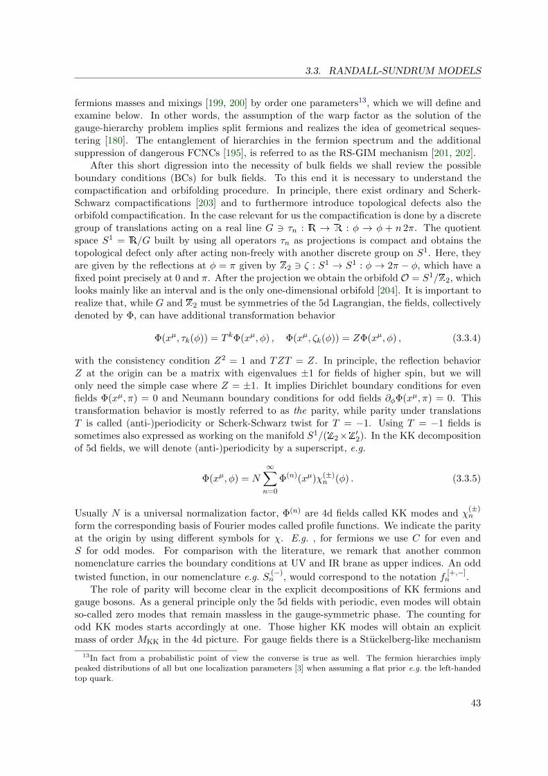
3.3. RANDALL-SUNDRUM MODELS
fermions masses and mixings [199, 200] by order one parameters13, which we will define andexamine below. In other words, the assumption of the warp factor as the solution of thegauge-hierarchy problem implies split fermions and realizes the idea of geometrical seques-tering [180]. The entanglement of hierarchies in the fermion spectrum and the additionalsuppression of dangerous FCNCs [195], is referred to as the RS-GIM mechanism [201, 202].
After this short digression into the necessity of bulk fields we shall review the possibleboundary conditions (BCs) for bulk fields. To this end it is necessary to understand thecompactification and orbifolding procedure. In principle, there exist ordinary and Scherk-Schwarz compactifications [203] and to furthermore introduce topological defects also theorbifold compactification. In the case relevant for us the compactification is done by a discretegroup of translations acting on a real line G 3 τn : R → R : φ → φ + n 2π. The quotientspace S1 = R/G built by using all operators τn as projections is compact and obtains thetopological defect only after acting non-freely with another discrete group on S1. Here, theyare given by the reflections at φ = π given by Z2 3 ζ : S1 → S1 : φ → 2π − φ, which have afixed point precisely at 0 and π. After the projection we obtain the orbifold O = S1/Z2, whichlooks mainly like an interval and is the only one-dimensional orbifold [204]. It is important torealize that, while G and Z2 must be symmetries of the 5d Lagrangian, the fields, collectivelydenoted by Φ, can have additional transformation behavior
Φ(xµ, τk(φ)) = T kΦ(xµ, φ) , Φ(xµ, ζk(φ)) = ZΦ(xµ, φ) , (3.3.4)
with the consistency condition Z2 = 1 and TZT = Z. In principle, the reflection behaviorZ at the origin can be a matrix with eigenvalues ±1 for fields of higher spin, but we willonly need the simple case where Z = ±1. It implies Dirichlet boundary conditions for evenfields Φ(xµ, π) = 0 and Neumann boundary conditions for odd fields ∂φΦ(xµ, π) = 0. Thistransformation behavior is mostly referred to as the parity, while parity under translationsT is called (anti-)periodicity or Scherk-Schwarz twist for T = −1. Using T = −1 fields issometimes also expressed as working on the manifold S1/(Z2×Z′2). In the KK decompositionof 5d fields, we will denote (anti-)periodicity by a superscript, e.g.
Φ(xµ, φ) = N
∞∑
n=0
Φ(n)(xµ)χ(±)n (φ) . (3.3.5)
Usually N is a universal normalization factor, Φ(n) are 4d fields called KK modes and χ(±)n
form the corresponding basis of Fourier modes called profile functions. We indicate the parityat the origin by using different symbols for χ. E.g. , for fermions we use C for even andS for odd modes. For comparison with the literature, we remark that another commonnomenclature carries the boundary conditions at UV and IR brane as upper indices. An odd
twisted function, in our nomenclature e.g. S(−)n , would correspond to the notation f
[+,−]n .
The role of parity will become clear in the explicit decompositions of KK fermions andgauge bosons. As a general principle only the 5d fields with periodic, even modes will obtainso-called zero modes that remain massless in the gauge-symmetric phase. The counting forodd KK modes starts accordingly at one. Those higher KK modes will obtain an explicitmass of order MKK in the 4d picture. For gauge fields there is a Stuckelberg-like mechanism
13In fact from a probabilistic point of view the converse is true as well. The fermion hierarchies implypeaked distributions of all but one localization parameters [3] when assuming a flat prior e.g. the left-handedtop quark.
43

3. THEORETICAL CLASSIFICATION & EXAMPLES OF NEW PHYSICS
[205] at work that involves the fifth component of the gauge fields as the corresponding scalarmode. The zero modes in turn obtain mass only after electroweak symmetry breaking throughinsertions of the Higgs VEV and further mixings with other KK modes that are also generatedby electroweak symmetry breaking. This resolves a great obstacle in the implementation ofchiral low-mass 4d fermions. In principle, chirality projections do not exist for fields in oddspace-time dimensions, the reason being that the Clifford algebra relation γM , γN = 2ηMN1in n = 2ν and n = 2ν + 1 dimensions can be fulfilled by n matrices of size 2ν × 2ν [206]. Thegraduating automorphism γ5 that distinguishes the two chiral representations in 4d is partof the Clifford algebra in 5d and part of the 5d representation of the Lorentz-group for Diracfermions to generate translations in φ-direction. However, we can resemble chiral fermions byassigning an odd parity to the wrong chirality of fermions, i.e. to right-handed doublets andleft-handed singlets. Remark that the spectrum of heavy fermion modes will thus contain atleast twice as many degrees of freedom per KK modes compared to the SM-fermion spectrum.
Much like periodic, odd modes, also anti-periodic modes of both parity do not possess azero mode and all modes obtain mass of order MKK. This combination of boundary conditionsturns out to be useful to give exotic fermions a heavy KK spectrum and to break additionalgauge symmetries by a combination of periodic and anti-periodic boundary conditions as wewill discuss in section 3.3.5.
We shortly come back to the remaining Higgs sector, which is confined to the IR brane witha function δ(φ−π) in the setup we consider below. The 5d Yukawa coupling of the Higgs bosonpresents a localized source in the 5d equations of motion (EOMs) for fermions and distortsthe fermion profiles. The presence of a δ-function seemingly leads to jump conditions wellknown from simple quantum mechanics problems. This is referred to as modified boundaryconditions for the fermions. To clarify this terminology a comment is in order. We will showin section 3.3.8.1 that a proper regularization of the δ-function used to regularize the Higgsboson, is essential to obtain correct 4d Yukawa couplings [4, 207]. This is done with the usualweak limit of smooth kernel functions, extending infinitesimally into the bulk, which define theδ-distribution in the limit of a regularization parameter η approaching 0. In the regularizedtheory, only smooth functions are involved and thus the boundary conditions remain exactlyNeumann or Dirichlet. Only in the limit of η → 0, odd profile functions may develop a valuelimε→0 S(π − ε) 6= 0 whilst S(π) = 0 remains true. We denote the limiting value also withS(π−), as it enters many relevant quantities.
3.3.3 Fermions in a Curved Background
In order to treat fermions in a curved background we give a short digression into the formaltreatment of their general action. Spinor formalism in a general curved background canbe conveniently expressed in the vielbein formalism. Roughly spoken, the inverse vielbeine Aa = diag(eσ(φ), . . . , eσ(φ), 1) represents the local coordinate system. Analogous to the Levi-
Civita-connection ΓNMP for the treatment of gravity in the framework of general relativity, wealso need its generalization, the so-called spin connection ωbcA. Geometrically it is a mixedobject from Lie
(SO(1, 4)
)⊗ Λ1M , where M is our 5d manifold. It represents the induced
unique, metric, and torsion-free Levi-Civita-connection of M inside the spinor bundle. Thatsaid the action of a single Dirac spinor ψ is given by
SF =
∫dΩ
[e Aa
(i
2ψγa
↔∂Aψ +
1
8ωbcAψ γa, σbcψ
)−m sgn(φ) ψψ
]. (3.3.6)
44
3.3. RANDALL-SUNDRUM MODELS
We have used the general measure of a curved space dΩ = d4x r dφ√G, where in the RS
background G = e−8σ is the determinant of the metric. Observe that for the mass term tobe non-vanishing, we have to assign an odd parity to it, so an additional sign function wasincluded. A thorough discussion of the action can be found in [208]. We indicate that thespin connection can easily be calculated with the non-zero Christoffel symbols
Γµ5ν = Γµν5 = −σ′(φ)δµν , Γ5µν = −e−2σ(φ)σ′(φ)ηµν (3.3.7)
as
ωM =1
4ωabMγaγb =
1
4ηbc(∂Me
Nc
)e aN + e a
N ΓNMP ePc
γaγb
= (1− δM5)σ′(φ)e−σ(φ)
2δaMγaγ5
(3.3.8)
It gives in fact no contribution to the action [186] since
e Aa γa, ωA ∝ δAa γa, δbAγbγ5 = 0 . (3.3.9)
We postpone the further treatment of (3.3.6) to the discussion of the model-specific imple-mentations given below.
3.3.4 Minimal Randall-Sundrum Model
In the following, we consider the gauge and fermion sector of the minimal realization of aRS model that reproduces the SM field content as zero modes. We will discuss the KKdecomposition for the electroweak and fermion sector. The extension to the QCD sector isstraightforward.
3.3.4.1 Gauge-Boson Sector
In the simplest version, we consider a SU(2)L×U(1)Y gauge theory, coupled to a scalar sectoron the IR brane. As explained in the last section, the vector components W a
µ and Bµ have tobe even under the Z2 orbifold symmetry and in order to remove the scalar components W a
φ
and Bφ from the low energy spectrum they are chosen to be odd. The action can be split upas
SG =
∫d4x r
π∫
−π
dφ(LV + LH + LGF + LFP
), (3.3.10)
where
LV =
√G
rGKMGLN
(−1
4W aKLW
aMN −
1
4BKLBMN
), (3.3.11)
LH =δ(|φ| − π)
r
[(DµΦ)† (DµΦ)− V (Φ)
], V (Φ) = −µ2Φ†Φ + λ
(Φ†Φ
)2(3.3.12)
are the Lagrangian for the 5d gauge theory and brane-localized Higgs sector. We replace four-component indices with five-component capital indices and denote the 5d metric as GMN .We use the same notation as in the SM (2.2.6) for the components of the Higgs doublet afterelectroweak symmetry breaking and we apply the usual rotation with a weak mixing angle,
45

3. THEORETICAL CLASSIFICATION & EXAMPLES OF NEW PHYSICS
defined here via the 5d gauge couplings as tan(θw) ≡ g′5/g5, to arrive at the fields AM and ZM .The kinetic terms for the Higgs field give rise to 5d mass terms MW 5 = vg5/2 = MZ5cw ofmass dimension 1/2, and bilinear terms involving the gauge and would-be Goldstone bosons.Moreover, the kinetic terms for the gauge fields in (3.3.11) also contain bilinear terms of thegauge bosons and their scalar components W±φ , Zφ, and Aφ. All of these mixed terms can beremoved with a suitable choice of the gauge-fixing Lagrangian [1]
LGF = − 1
2ξ
(∂µAµ − ξ
[∂φ e
−2σ(φ)Aφr2
])2
− 1
2ξ
(∂µZµ − ξ
[δ(|φ| − π)
rMZ5 ϕ
3 +∂φ e
−2σ(φ)Zφr2
])2
− 1
ξ
(∂µW+
µ − ξ[δ(|φ| − π)
rMW 5 ϕ
+ +∂φ e
−2σ(φ)W+φ
r2
])
×(∂µW−µ − ξ
[δ(|φ| − π)
rMW 5 ϕ
− +∂φ e
−2σ(φ)W−φr2
]).
(3.3.13)
Note that there is no problem in squaring the δ-functions. We will see below that the deriva-tives of the scalar components of the gauge fields W±φ and Zφ also contain a δ-functioncontribution, which precisely cancels the δ-functions from the Higgs sector. As a result, con-trary to the treatment in [209], we do not need to introduce separate gauge-fixing Lagrangiansin the bulk and on the IR brane. Such a separate treatment is useful when considering the5d propagator of gauge bosons as discussed in section 3.3.7 in general Rξ gauge [210]. Thebilinear terms in the action now read
SG,2 =
∫d4x r
π∫
−π
dφ
− 1
4FµνF
µν − 1
2ξ(∂µAµ)2
+e−2σ(φ)
2r2[∂µAφ∂
µAφ + ∂φAµ∂φAµ]− ξ
2
[∂φ e
−2σ(φ)Aφr2
]2
− 1
4ZµνZ
µν − 1
2ξ(∂µZµ)2 +
e−2σ(φ)
2r2[∂µZφ∂
µZφ + ∂φZµ∂φZµ]
− 1
2W+µνW
−µν − 1
ξ∂µW+
µ ∂µW−µ +e−2σ(φ)
r2
[∂µW
+φ ∂
µW−φ + ∂φW+µ ∂φW
−µ]
(3.3.14)
+δ(|φ| − π)
r
[1
2∂µh∂
µh− λv2h2 + ∂µϕ+∂µϕ− +
1
2∂µϕ
3∂µϕ3 +M2Z5
2ZµZ
µ +M2W 5W
+µ W
−µ]
− ξ
2
[δ(|φ| − π)
rMZ5 ϕ
3 +∂φ e
−2σ(φ)Zφr2
]2
− ξ[δ(|φ| − π)
rMW 5 ϕ
+ +∂φ e
−2σ(φ)W+φ
r2
][δ(|φ| − π)
rMW 5 ϕ
− +∂φ e
−2σ(φ)W−φr2
]+ LFP
.
The form of the Faddeev-Popov ghost Lagrangian is analogous to that of the SM, with theonly generalization that a ghost field is required for every KK mode.
46
3.3. RANDALL-SUNDRUM MODELS
The KK decompositions of the 5d fields has the general form
Vµ(x, φ) =1√r
∑
n
V (n)µ (x)χ
(+)V,n(φ) , Vφ(x, φ) =
1√r
∑
n
aVn ϕ(n)V (x) ∂φ χ
(+)V,n(φ) , (3.3.15)
where V = A,Z,W±. V(n)µ are the 4d mass eigenstates, the various χ
(+)V,n profiles form
complete sets of even functions on the orbifold, which obey orthonormality conditions on S1
with respect to the measure dφ. The superscript (+) indicates untwisted, i.e. periodic modes,and aVn are coefficients, which we determine below. The choice of ∂φ χ
Vn as modes for the
scalar fifth components is a viable ansatz since it automatically reverses the BCs. It is in factalso necessary as one can easily show. The 5d scalar fields also have to be expanded in thebasis of 4d mass eigenstates. To associate a scalar Goldstone mode with each KK level wewrite
ϕ±(x) =∑
n
bWn ϕ±(n)W (x) , ϕ3(x) =
∑
n
bZn ϕ(n)Z (x) , (3.3.16)
and determine the coefficients bVn below. We will denote the masses of 4d vector fields by
mVn ≥ 0. As usual the masses of scalar fields ϕ
(n)V will be related to these by gauge invariance.
Inserting these decompositions into the action, one finds that the profiles χan obey the 5dequation of motion [185, 193]
− 1
r2∂φ e
−2σ(φ) ∂φ χ(+)V,n(φ) = (mV
n )2 χ(+)V,n(φ)− δ(|φ| − π)
rM2V 5 χ
(+)V,n(φ) . (3.3.17)
In summary we have to find the spectrum of the differential operator − 1r2 ∂φ e
−2σ(φ)∂φ on[0, π] subject to the boundary conditions
∂φ χ(+)V,n(0) = 0 , ∂φ χ
(+)V,n(π−) = −rM
2V 5
2ε2χ
(+)V,n(π) . (3.3.18)
The superscript notation π− signifies the left limiting value of the function at the IR brane.
Note that the derivative of χ(+)V,n becomes discontinuous at π due to (3.3.17). The appro-
priate IR BCs for the profiles have been obtained by integrating the EOM (3.3.17) over aninfinitesimal interval around |φ| = π and carrying out the regulating limit involved in the
definition of the δ-function. Remark that the IR BCs force the profile to be χ(+)V,n to be non-
smooth at φ = π. Since the profiles of the scalar components are taken to be proportionalthe φ-derivative of the vector profiles, they develop discontinuities at the IR brane.
We find that the action takes the desired form
SG,2 =∑
n
∫d4x
− 1
4F (n)µν F
µν(n) − 1
2ξ
(∂µA(n)
µ
)2+
(mAn )2
2A(n)µ Aµ(n)
− 1
4Z(n)µν Z
µν(n) − 1
2ξ
(∂µZ(n)
µ
)2+
(mZn )2
2Z(n)µ Zµ(n)
− 1
2W+(n)µν W−µν(n) − 1
ξ∂µW+(n)
µ ∂µW−(n)µ + (mW
n )2W+(n)µ W−µ(n)
+1
2∂µϕ
(n)A ∂µϕ
(n)A −
ξ(mAn )2
2ϕ
(n)A ϕ
(n)A +
1
2∂µϕ
(n)Z ∂µϕ
(n)Z −
ξ(mZn )2
2ϕ
(n)Z ϕ
(n)Z
+ ∂µϕ+(n)W ∂µϕ
−(n)W − ξ(mW
n )2 ϕ+(n)W ϕ
−(n)W
+
∫d4x
(1
2∂µh∂
µh− λv2h2
)+∑
n
∫d4xL(n)
FP ,
(3.3.19)
47

3. THEORETICAL CLASSIFICATION & EXAMPLES OF NEW PHYSICS
if and only if
aVn = − 1
mVn
, bVn =MV 5√r
χ(+)V,n(π−)
mVn
. (3.3.20)
The resulting theory contains a tower of massive gauge bosons with masses mVn , accompanied
by a tower of massive scalars with masses√ξ mV
n , as well as the Higgs field h with mass√2λv. Note that with (3.3.20) the 4d gauge-fixing Lagrangian derived from (3.3.13) takes
the simple form
r
π∫
−π
dφLGF =∑
n
L(n)GF , (3.3.21)
with
L(n)GF = − 1
2ξ
(∂µA(n)
µ − ξmAnϕ
(n)A
)2− 1
2ξ
(∂µZ(n)
µ − ξmZnϕ
(n)Z
)2
− 1
ξ
(∂µW+(n)
µ − ξmWn ϕ
+(n)W
)(∂µW−(n)
µ − ξmWn ϕ−(n)W
).
(3.3.22)
For each KK mode these expressions are identical to those of the SM. It follows that the form
of the Faddeev-Popov ghost Lagrangians L(n)FP in (3.3.19) is analogous to that of the SM, with
the only generalization that a ghost field is required for every KK mode.
3.3.4.2 Fermion Sector
For the minimal embedding of fermions we consider the SM gauge-representations and quan-tum numbers, however using Dirac fermions because of the absence of the chiral represen-tation of the Lorentz group in 5d as discussed in section 3.3.2. Instead we give appropriateZ2-parities to the formally defined chiral projections PL,R = (1−γ5)/2 of the vector-like Diracfermions, i.e. for the SU(2)L doublets we give even parity to the left-handed and odd parityto the right-handed chirality and vice versa for the fermion singlets.
We denote the components of SU(2)L doublets by u, d and singlets by u c, d c and consideronly quarks for the moment. We generalize the fermion action (3.3.6) and add Yukawainteractions with the IR-brane Higgs boson that have the same form like in the SM. Thebilinear part of the fermion action can then be written as [186, 195]
SF,2 =
∫d4x r
π∫
−π
dφ
∑
q=U,u,D,d
(e−3σ(φ) ~q i/∂ ~q − e−4σ(φ) sgn(φ) ~qM~q ~q
− 1
2r
[~qL e
−2σ(φ)↔∂φ e
−2σ(φ) ~qR + h.c.])
− δ(|φ| − π) e−3σ(φ) v√2r
∑
(Q,q)=(U,u),(D,d)
[~QL Y
(5d)~q ~qR + ~QR Y
(5d)o ~q ~qL + h.c.
],
(3.3.23)
with↔∂φ ≡
→∂φ −
←∂φ and we used a generalized notation that will facilitate the transition to
more complicated fermion embeddings. For the minimal model the notation reduces triviallyto
~U ≡ u , ~D ≡ d , M~U = M ~D ≡MQ ,
~q ≡ qc , M~q = Mq , Y(5d)
(o)~q ≡ Y(5d)
(o)q , (q = u, d) .(3.3.24)
48

3.3. RANDALL-SUNDRUM MODELS
Canonical kinetic terms and flavor-diagonal and real masses in (3.3.23) have been achievedby appropriate unitary transformations of the quark fields, so the given form stands withoutloss of generality. In contrast to the SM where fermion masses solely come from the Yukawainteractions, we cannot exclude negative diagonal entries in the mass matrices. Indeed, phe-nomenologically it turns out that the definitions
cQ ≡1
kMQ , cq ≡ −
1
kMq (3.3.25)
are useful, since all quarks except the top quark will be clustered around cQ,q ≈ 1/2.
In principle, there are two different types of Yukawa matrices either for two Z2-even orZ2-odd fermions. The latter has been neglected in [1] and all the literature before since itdoes naively not contribute because of the Dirichlet BCs at the IR brane. Indeed, the correctspectrum can be inferred by neglecting this type of Yukawa matrices. However, in [207] it wasrecognized that they are essential to derive the correct Higgs–fermion couplings. Consideringthe brane-localized Higgs sector as the limit of a bulk Higgs boson, 5d Lorentz invariance
renders both types of Yukawa matrices identical Y(5d)
(o) ~q = Y(5d)~q . We will adopt this choice
in the following. In the decomposition it will be useful to furthermore define dimensionlessYukawa matrices
Y~q ≡k
2Y
(5d)~q , (q = u, d) . (3.3.26)
The entries of this matrix shall take naturally non-hierarchical, complex values of O(1).The hierarchies of the Yukawa matrices of the SM quarks in the effective 4d theory areexplained in terms of a geometrical realization of the Froggatt-Nielsen mechanism in RSmodels [1, 200, 211, 212].
Of course, we can also shed light on the remaining leptons by localization in the bulk. Forinstance one of the first ideas in considering fermionic fields in the RS bulk was how to obtainsmall and phenomenologically viable neutrino masses. This can be done by introducingtwo right-handed sterile neutrinos that live in the bulk [186] and additionally suppressingcontributions from higher dimensional operators, by very small brane values of the modes[195].
For the KK decomposition we use a compact notation [2], in which the profile functionsof the left-handed (right-handed) interaction eigenstates that can mix into the left-handed
(right-handed) components of the 4d mass eigenstates are collected in vectors Q(n)A (t). They
are defined in terms of the KK decompositions
√r
(ε
t
)2( ~QL(x, t)~qL(x, t)
)=∑
n
(CQn (t)~aQnSqn(t)~aqn
)q
(n)L (x) ≡
√Lε
2π
∑
n
Q(n)L (t) q
(n)L (x) ,
√r
(ε
t
)2( ~QR(x, t)~qR(x, t)
)=∑
n
(SQn (t)~aQnCqn(t)~aqn
)q
(n)R (x) ≡
√Lε
2π
∑
n
Q(n)R (t) q
(n)R (x) .
(3.3.27)
In this formula Q, q, and Q are assumed to take the values U , u, and U for the up-sector, or D,d, and D for the down sector, etc. . In the minimal model, the generalized vectors with capitalletters contain SU(2)L-doublet components and those with small letters the singlets. Thus,the combined notation expresses mixing between KK modes and singlet–doublet mixing dueto electroweak symmetry breaking, both in the same compact form. We anticipate that thevectors will be extended even further in the custodial model, where additional 5d quarks with
49

3. THEORETICAL CLASSIFICATION & EXAMPLES OF NEW PHYSICS
twisted BCs are introduced, yet, the notation of (3.3.27) is general enough to accommodatealso this extended case. In (3.3.27), we directly switched to t-coordinate notation (see (3.3.2)and text before) and extracted normalization factors that simplify the following expressions.CQ,qn (t) and SQ,qn (t) are diagonal matrices of even and odd profile functions and ~aQ,qn are
decomposition vectors that parametrize the full mixing implied by electroweak symmetrybreaking. The symbols Q, q are understood to take either the values U, u or D, d here. In theminimal RS model, this general notation again breaks down to equivalent values for the 3× 3matrices of the profile functions of the doublet fermions
CUn (t) = CD
n (t) ≡ CQ(+)n (t) , SUn (t) = SDn (t) ≡ SQ(+)
n (t) , (3.3.28)
where the superscript (+) indicates untwisted profiles. There are three zero modes in theup and down sector that represent the SM-like fermions. Each higher KK level containssix modes with O(v) mass splittings, while the different levels are split by an amount ofO(MKK). We choose the index n to enumerate all these modes subsequently, i.e. 1 − 3 forthe zero modes 4 − 9 for the KK modes of the first level, etc. Remark that ~QL,R(x, φ) can
be expanded in terms of the same vector ~aQn . With this choice, the even and odd profilesCQn (φ) and SQn (φ) will be normalized in the same way. The same holds for Q → q. The
orthonormality conditions for the new vectors read
1∫
ε
dtQ(m)†σ (t)Q(n)
σ (t) = δmn , (3.3.29)
∑
n
Q(n)σ (t)Q(n)†
σ (t′) = δ(t− t′) , (3.3.30)
where σ = L,R. A thorough discussion of the individual normalization of the profiles CQn (φ)
and SQn (φ) can be found in [4], but we refrain from repeating it here. However, note that it isimportant to realize that the individual profiles CQ,q
n ~aQ,qn do not satisfy relations analogousto (3.3.29) and (3.3.30). This non-orthogonality is intuitive since the modes of differentchiralities are mixed in the mass eigenstate basis, however it is not uniquely distributed onthe profiles CQ,q
n and eigenvectors ~aQ,qn . The split into these two quantities is in fact onlynecessary in order to derive analytic expressions for the profiles and to clearly separate themixing into ~aQ,qn = ~en/
√2 +O(v2/M2
KK), with unit vectors ~en. The choice to normalize themixing vectors as (
~aQn)†~aQn +
(~a qn)†~a qn = 1 , (3.3.31)
fixes the analytic form of the profiles, which we give below in section 3.3.6.The 5d variational principle requires all the variations of the action (3.3.23) to vanish
for arbitrary infinitesimal changes of the fermionic fields. It is straightforward to see thatthe EOMs for 5d Dirac fermions lead to the following EOMs for the profiles after the KKdecomposition [4]
δSf
δ( ~Qσ, ~qσ)T:
((−1)δσR ∂t +Mq(t)
)Q(n)σ (t) = xnQ(n)
σ (t) , (σ = L,R) . (3.3.32)
Here, xn = mqn/MKK are the mass eigenvalues, σ denotes the opposite chirality and
Mq(t) =1
t
(c ~Q 0
0 −c~q
)+ δη(t− 1)
v√2MKK
(0 Y~qY †~q 0
), (3.3.33)
50
3.3. RANDALL-SUNDRUM MODELS
is the generalized mass matrix. Remark that we have added the regularization parameter ηto the notation of the δ-function. It has been emphasized in [207] that in order to properlyevaluate the Yukawa couplings this careful treatment is essential. The reason is that with abrane-localized Higgs sector the odd fermion profiles SQ,qn (t) are discontinuous at t = 1 [213],and hence the overlap integral of a product of two such functions with the naive Higgs profileδ(t− 1) is in fact ill defined. In the following, we will therefore consider the δ-function as theweak limit of a sequence of normalized, regularized functions δη with support on the intervalx ∈ [−η, 0] as
limη→0+
+∞∫
−∞
dx δη(x)f(x) = f(0) , (3.3.34)
for all test functions f(x), i.e. smooth functions of compact support. The precise shape ofthis function will be irrelevant.
Due to the regularization of the Higgs profile the simple Dirichlet boundary conditionshold like in the case of a bulk Higgs boson
(0 1
)Q(n)L (t) = 0 =
(1 0
)Q(n)R (t) for t = ε, 1 . (3.3.35)
Within the bulk and away from the support of the Higgs profile, i.e. , for t < 1 − η, thegeneral solutions [186, 195] to the EOMs (3.3.32) can be written as linear combinations ofBessel functions, which we discuss below in section 3.3.6. The appearance of the regularizedHiggs profile δη(t− 1) as a source in (3.3.32) however renders the solutions for t > 1− η, i.e.close to the brane, completely different. In the following we derive the solution for η 1.In this case the Higgs profile source terms in the EOM (3.3.32) are dominant δη ∼ 1/η andas a result the behavior of the profiles CQ,q
n (φ) and SQ,qn (φ) become independent of the massterms. Then, the integral version of the 1/η components of the EOM reads
Q(n)σ (t)−Q(n)
σ (1) = (−1)δσLv√
2MKK
(0 Y~qY †~q 0
) 1∫
t
dt′ δη(t′ − 1)Q(n)σ (t′) . (3.3.36)
In order to solve (3.3.36), we first introduce the regularized Heaviside function
θη(x) ≡ 1−x∫
−∞
dy δη(y) , (3.3.37)
which obeys ∂x θη(x) = −δη(x) and has the values θη(0) = 0, and θη(−η) = 1. Using the
latter properties it is readily shown that
1∫
t
dt′ δη(t′ − 1) θη(t′ − 1)n =1
n+ 1θη(t− 1)n+1 . (3.3.38)
Thus for any arbitrary invertible matrix A one has
1∫
t
dt′ δη(t′ − 1) sinh(θη(t′ − 1)A
)=(
cosh(θη(t− 1)A
)− 1)A−1 ,
1∫
t
dt′ δη(t′ − 1) cosh(θη(t′ − 1)A
)= sinh
(θη(t− 1)A
)A−1 ,
(3.3.39)
51

3. THEORETICAL CLASSIFICATION & EXAMPLES OF NEW PHYSICS
where the hyperbolic sine and cosine are defined via their power expansions. These relationsdirectly show the solution to the Peano-iteration of (3.3.36)
Q(n)L (t) =
√2π
Lε
cosh
(θη(t− 1) v√
2MKK
√Y~qY
†~q
)CQn (1)~aQn
−Y †~q(√
Y~qY†~q
)−1
sinh
(θη(t− 1) v√
2MKK
√Y~qY
†~q
)CQn (1)~aQn
,
Q(n)R (t) =
√2π
Lε
Y †~q
(√Y~qY
†~q
)−1
sinh
(θη(t− 1) v√
2MKK
√Y~qY
†~q
)Cqn(1)~aqn
cosh
(θη(t− 1) v√
2MKK
√Y~qY
†~q
)Cqn(1)~aqn
.
(3.3.40)
The six components of Q(n)L are both determined by the three boundary values CQ
n (1)~aQn . Thisimplies a relation between the components. In this sense (3.3.40) represents the regularizedanaloga to the IR BC for gauge bosons (3.3.18). In the latter case, we were able to directlywork with the naive description of the δ-function. Here, we will see effectively a similar result.The correct treatment of the δ-function finally only amounts to a redefinition of the Yukawamatrix as far as the KK spectrum is concerned. This is seen as follows. The non-trivialconnecting condition between the usual form of the solution and the one derived here is nowlocated at t = 1 − η. At this point we evaluate (3.3.40) and eliminate the on-brane valuesCQ,qn (1). Introducing the rescaled Yukawa matrices
Y~q ≡ X~qX−1~q Y~q , X~q ≡
v√2MKK
√Y~q Y
†~q , X~q = tanh(X~q) , (3.3.41)
which coincide at leading order with the original ones, i.e. Y~q = Y~q +O(v2/M2KK), we obtain
the IR BCs
(v√
2MKK
Y †q 1
)Q(n)L (1− η) = 0 ,
(1 − v√
2MKK
Yq
)Q(n)R (1− η) = 0 , (3.3.42)
Hence, they take precisely the same form as in [1], with the original Yukawa couplings replacedby the rescaled ones as defined in (3.3.41). Since in practice the Yukawa matrices (togetherwith the quark profiles) are chosen such that the zero-mode masses as well as the quarkmixing angles match the ones determined by experiment, such a rescaling has no observableeffect on the mass spectrum and the mixing pattern. However, as we will explain in moredetail below, the inclusion of the Yukawa coupling involving Z2-odd fermions alters the formof the tree-level interactions of the Higgs boson with fermions.
Finally, the mass eigenvalues mn follow from the solutions to the equation
det
(1 +
v2
2M2KK
Y~qCqn(π−)
[S qn(π−)
]−1Y †~q C
Qn (π−)
[SQn (π−)
]−1)
= 0 . (3.3.43)
Once they are known, the eigenvectors ~aQ,qn can be determined from (3.3.42). Note that, whileit is always possible to work with real and diagonal profiles CQ,q
n (φ) and SQ,qn (φ), the vectors~aQ,qn are, in general, complex-valued objects.
52

3.3. RANDALL-SUNDRUM MODELS
3.3.5 Custodial Randall-Sundrum Model
3.3.5.1 Gauge-Boson Sector
As an extension to the discussion in 3.3.4.1, we also consider the RS model as proposed in[214, 215] with the custodial symmetry of the SM Higgs sector as a full bulk gauge symmetryO(4)×U(1)X ∼ SU(2)L×SU(2)R×U(1)X×PLR. The rationale for the left-right parity PLRwill be explained below when discussing fermions. However, we will allow for explicit sourcesof PLR violation in the following and comment on them. The action reads
SG =
∫d4x r
π∫
−π
dφ(LL,R,X + LH + LGF
), (3.3.44)
with the gauge-kinetic terms
LL,R,X =
√G
rGKMGLN
(−1
4LaKLL
aMN −
1
4RaKLR
aMN −
1
4XKLXMN
). (3.3.45)
The 5d gauge couplings are denoted by gL,R,X5. We furthermore define the dimensionless
4d gauge couplings as ga = ga5/√
2πr. The choice of Z2-parity, for vector and scalar fifthcomponent are again even and odd respectively. The Higgs Lagrangian is given by
LH =δ(|φ| − π)
r
(1
2Tr∣∣(DµΦb)
∣∣2 − V (Φb)
)(3.3.46)
We employ the symmetry-breaking pattern SU(2)L × SU(2)R → SU(2)V to the diagonalsubgroup by using a Higgs bidoublet in the real representation (2, 2)0. This scheme providesa custodial symmetry, which protects the T parameter. Additionally PLR symmetry preventsthe left-handed Zbb coupling from receiving excessively large corrections [216]. On the UVbrane, the symmetry breaking SU(2)R × U(1)X → U(1)Y is achieved by a mixture of UVand IR BCs. Remark that in contrast to left-right symmetric models that employ a breakingpattern to a diagonal SU(2) subgroup [217–221], where this step is taken at a scale u v inaddition to the usual Higgs mechanism, the breaking pattern here is fundamentally different.It rather resembles the pattern of composite Higgs models [222], e.g. the Little Higgs modelsdiscussed in section 3.2, where the Higgs sector LH is SM-like, the only difference being thegauged custodial symmetry. In particular the same number of degrees of freedom are usedby rewriting the complex representation Φ ∼ (1, 2)Y=1/2, used by the SM Higgs mechanism,
to a real bifundamental Φb = (Φc,Φ) ∼ (2, 2)0 with approximately14 the same diagonal VEV⟨Φb⟩
= v/√
2 1. Accordingly, SU(2)L transformations act from the left on the bidoublet,while the SU(2)R transformations act from the right. Using T iL,R = σi/2, the covariantderivative in the Higgs sector reads
DµΦb = ∂µΦb − igL5 Liµ T
iL Φb + igR5 ΦbRiµ T
iR
=1√2
(∂µ(h− iϕ3
)− i v2
(gL5 L
3µ − gR5R
3µ
)−∂µi
√2ϕ+ − i v2
(gL5 L
+µ − gR5R
+µ
)
−∂µi√
2ϕ− − i v2(gL5 L
−µ − gR5R
−µ
)∂µ(h+ iϕ3
)+ i v2
(gL5 L
3µ − gR5R
3µ
))
+ terms bilinear in fields , (3.3.47)
14We will see below that a tree-level contribution to the W -mass slightly shifts the VEV.
53

3. THEORETICAL CLASSIFICATION & EXAMPLES OF NEW PHYSICS
The structure of (3.3.47) shows that the mass matrix is diagonalized by defining the newfields [223] (
AiMV iM
)=
(cW −sWsW cW
)(RiMLiM
)≡ RW
(RiMLiM
), tW =
gRgL
. (3.3.48)
Afterwards, the 5d mass term adopts the form
LG,mass =δ(|φ| − π)
r
(g2L5 + g2
R5
)v2
8AiµA
µ i ≡ δ(|φ| − π)
r
1
2M2A5AiµA
µ i . (3.3.49)
This explicitly shows the IR brane induced breaking pattern SU(2)L × SU(2)R → SU(2)V .The mixing angle θW introduced in (3.3.48) is the only rotation we need in the 5d chargedsector. The zero mode of the coupled system ~W±M = (A±M , V
±M )T will resemble the SM-like
W±. The rotations in the neural sector are more intricate as we discuss in the following.We mentioned above that appropriate BCs on the UV brane break the extended elec-
troweak gauge group down to the SM gauge group SU(2)R × U(1)X → U(1)Y . Explicitly,this is done as follows. We introduce the new fields
(BMZ ′M
)=
1√g2R + g2
X
(gR gX−gX gR
)(XM
R3M
), (3.3.50)
and give Dirichlet BCs to Z ′µ and R1,2µ on the UV brane. The SM-like neutral electroweak
gauge bosons are defined in the standard way with the U(1)Y hypercharge coupling given byg−2Y = g−2
R + g−2X , such that
(AMZM
)=
(cw sw−sw cw
)(BML3M
), tw =
gYgL
, (3.3.51)
and we give Neumann BCs to Zµ, Aµ and L1,2µ on the UV brane. The different choice of BCs
explicitly breaks the mentioned symmetry and makes the necessity of Scherk-Schwarz twistedKK modes apparent.
Finally, the fields V 3M and XM can be rotated to the photon field AM and a state ZHM via
(AMZHM
)=
1
g2LRX
gL gR gX
√g2L + g2
R
−gX√g2L + g2
R gL gR
(XM
V 3M
), (3.3.52)
where g4LRX = g2
L g2R + g2
L g2X + g2
R g2X . We also write ZM ≡ A3
M , as it is already the correctlinear combination of ZM and Z ′M , which is orthogonal to ZHM . The necessary rotation in the5d neutral sector for the Z boson is in summary given by
(ZMZHM
)=
(cZ −sZsZ cZ
)(ZMZ ′M
)≡ RZ
(ZMZ ′M
), tZ =
g2R
g2LRX
. (3.3.53)
The zero mode of the coupled system ~ZM = (ZM , ZHM )T will resemble the SM-like Z. Remark
that the three introduced angles cw, cW , cZ parametrize the weak mixing angle defined by theusual rotation of the U(1)Y in the U(1)em boson, the relative size of the two SU(2) gaugecouplings comparable to what is usually called cβ in multi-Higgs doublet models and e.g. theleft–right-symmetric model, and the third angle is dependent, c2
Z = c2W /c
2w.
54

3.3. RANDALL-SUNDRUM MODELS
SU(2)R × U(1)X → U(1)Y SU(2)L × SU(2)R → SU(2)V
∂φL±µ (x, 0) = 0 ∂φA
±µ (x, π−) = − r
2ε2M2A5A±µ (x, π)
R±µ (x, 0) = 0 ∂φV±µ (x, π) = 0
∂φZµ(x, 0) = 0 ∂φZµ(x, π−) = − r2ε2
M2A5Zµ(x, π)
Z ′µ(x, 0) = 0 ∂φZHµ (x, π) = 0
∂φAµ(x, 0) = 0 ∂φAµ(x, π) = 0
Table 3.3: UV and IR BCs in the gauge sector of the custodial RS model.
In table 3.3 we summarize the BCs at the two different branes that we choose for thefields in order to obtain the correct mass spectrum for the SM gauge bosons. We refer tothese sets of fields as the UV and IR basis, respectively. The BCs can easily be transformedbetween these two bases with the matrices RW,Z at the expense of obtaining expressions thatmix different fields. Remark that enforcing the PLR symmetry uniquely determines theserotations with cW = 1/
√2 and cZ = 1/
(√2cw). The photon Aµ has individual and source-
free Neumann BCs at both branes, and therefore its zero mode remains massless. Note thatthere is just one mass parameter MA entering the IR BCs, in contrast to the two parametersMZ and MW appearing in the minimal model. This is crucial for the custodial protectionof the T parameter. The different masses for the lightest electroweak gauge bosons are hereaccomplished through the mixed UV BCs of the gauge fields in the IR basis. As the Higgssector is localized on the IR brane, it is natural to work in the IR basis for that purpose.
The action of the theory still contains mixing terms between gauge fields and scalars,which can be removed by an appropriate gauge-fixing Lagrangian. It turns out that
LGF = − 1
2ξ
(∂µAµ − ξ
[∂φ e
−2σ(φ)
r2Aφ
])2
− 1
2ξ
(∂µ ~Zµ − ξ
[δ(|φ| − π)
rMA5
~ϕ 3 +∂φ e
−2σ(φ)
r2~Zφ
])2
− 1
ξ
(∂µ ~W+
µ − ξ[δ(|φ| − π)
rMA5
~ϕ+ +∂φ e
−2σ(φ)
r2~W+φ
])T
×(∂µ ~W−µ − ξ
[δ(|φ| − π)
rMA5
~ϕ− +∂φ e
−2σ(φ)
r2~W−φ
]),
(3.3.54)
is an appropriate choice.To perform the KK decomposition of the 5d fields, it is convenient to work with profiles
that obey definite Neumann (+) or Dirichlet (−) BCs at the UV brane, and parametrize themixing between the components of ~W±M (x, φ) and ~ZM (x, φ) that is induced by the IR BCs.Both advantages are elegantly combined by writing the KK decomposition as
~Vµ(x, φ) =RV√r
∑
n
χ+V,n(φ) ~AV
n V (n)µ (x) , ~Vφ(x, φ) =
RV√r
∑
n
∂φχ+V,n(φ) ~AV
n aVn ϕ
(n)V (x) ,
(3.3.55)where V = Z,W±, A. In fact, the decomposition of the photon A is the same as in (3.3.15)
and we account for this by setting RA = 1 and ~AAn = (1, 0)T . Note that V
(n)µ (x) are 4d mass
55
3. THEORETICAL CLASSIFICATION & EXAMPLES OF NEW PHYSICS
eigenstates and the lightest, zero modes are identified with the SM gauge bosons just like inthe structurally simpler decomposition of the minimal model (3.3.15). Mixing between theKK modes of V = W±, Z is encoded in the two-component vectors ~AVn , which are normalized
according to ( ~Aan)T ~Aan = 1. Furthermore, we have introduced the diagonal matrix
χ+V,n(φ) =
(χ
(+)V,n(φ) 0
0 χ(−)V,n(φ)
), (3.3.56)
The superscripts (+) and (−) label the type of BC we impose on the profiles at the UV brane.Remind from table 3.3 that both profiles satisfy an even BC at the IR brane, which we do notindicate explicitly to simplify the notation. The superscript therefore also indicates Scherk-Schwarz untwisted and twisted even functions. We also introduce the shorthand notations
~χVn (φ) =(χLV,n(φ), χRV,n(φ)
)T= χ+
V,n(φ) ~AVn , (3.3.57)
The profiles χ+V,n(φ) do not separately obey orthonormality conditions. This fact is related to
the decomposition of fields with Neumann and Dirichlet BCs into the same 4d gauge-bosonbasis and the implied mixing. This is analogous to the fermion decomposition of the minimalmodel discussed above. It is only the complete vectors ~χVn (φ) that are orthonormal andcomplete,
π∫
−π
dφ ~χVm(φ)T ~χVn (φ) = δmn , (3.3.58)
∑
n
~χVn (φ) ~χVn (φ)T =1
2
(δ(φ− φ′) + δ(φ+ φ′)
)1 . (3.3.59)
Note that the photon still obeys a standard orthonormality condition. To associate a scalarGoldstone mode with each KK level, again we expand the 5d Goldstone bosons in the basis
of 4d mass eigenstates ϕ(n)V (x) by [4]
~ϕ 3(x) =∑
n
~bZn ϕ(n)Z (x) , ~ϕ±(x) =
∑
n
~bWn ϕ±(n)W (x) . (3.3.60)
We insert the decomposition (3.3.55) into the action (3.3.44) and derive the followingEOMs [1, 185, 193] for the two component vectors of (3.3.57)
− 1
r2∂φ e
−2σ(φ)RV ∂φ ~χVn (φ) = (mV
n )2RV ~χVn (φ)− δ(|φ| − π)
rM2V 5P(+)RV ~χ
Vn (φ) , (3.3.61)
where V = Z,W,A the 5d masses are MZ5 = MW 5 = MA5, MA5 = 0, and we defined
the projectors P(+) = diag(1, 0) and P(−) = diag(0, 1). After an integration of (3.3.61)an infinitesimal region around the IR brane we obtain as the generalization of (3.3.18) thecondition
mVn
MKKRV χ
−V,n(π−) ~AV
n = −X2 LP(+)RV χ+V,n(π) ~AV
n , (3.3.62)
where
χ−V,n(φ) ≡ 1
mVn r
e−σ(φ)∂φχ+V,n(φ) , X2 ≡ (g2
L + g2R) v2
4M2KK
. (3.3.63)
56

3.3. RANDALL-SUNDRUM MODELS
Notice that for the photon the right-hand side in (3.3.62) is equal to zero.
After applying the EOMs and the orthonormality condition, we observe that the 4d actiontakes the desired canonical form, if and only if
aVn = − 1
mVn
, ~bVn =MV 5√rmV
n
P(+)RV ~χVn (π−) . (3.3.64)
The spectrum of the theory is determined by the IR BCs (3.3.62). Therefore, the numericaldetermination of the eigenvalues xVn ≡ mV
n /MKK is done by finding the solutions to thecharacteristic equation
det[xVn χ
−V,n(π−) + LX2DV χ
+V,n(π)
]= 0 ,
DV ≡ R−1V P(+)RV =
(c2V −sV cV
−sV cV s2V
).
(3.3.65)
Once the eigenvalues are known, the eigenvectors ~AVn are determined by (3.3.62).
3.3.5.2 Fermion Sector
The extended RS model shall also implement a custodial protection of the ZbLbL vertex [216]to comply with precision constraints from Z-pole observables in addition to the constraintsfrom the oblique T -parameter (see section 4.2.2). The fermion embedding shall thereforeadhere to a discrete PLR symmetry that interchanges the two SU(2) groups and the left-handed bottom quark has to be part of a SU(2)L × SU(2)R bidoublet with isospin quantumnumbers15 T 3
L = −T 3R = −1/2. This fixes the quantum numbers of the other fields and implies
the following, most economical multiplet structure for the quark fields with even Z2-parity:
QL ≡
u
(+)L 2
3λ
(−)L 5
3
d(+)L − 1
3u′ (−)L 2
3
23
, ucR ≡(uc (+)R 2
3
)23
,
TR ≡ T1R ⊕ T2R ≡
Λ′ (−)R 5
3
U′ (−)R 2
3
D′ (−)R − 1
3
23
⊕(D
(+)R − 1
3U
(−)R 2
3Λ
(−)R 5
3
)23
.
(3.3.66)
Again the superscript (−) denotes a Scherk-Schwarz twist. The inner and outer subscripts cor-respond to the electromagnetic and U(1)X charges, respectively, which are connected throughthe relations Y = −T 3
R +QX and Q = T 3L + Y . In addition to (3.3.66), we have a second set
of multiplets, belonging to the components of opposite chirality. The corresponding stateshave opposite BCs. In particular, they all obey Dirichlet BCs at the IR brane. The SU(2)L,Rtransformations act vertically and horizontally on the multiplets. We summarize the quantumnumbers of the quark fields in table 3.4. Note that we have chosen the same SU(2)L×SU(2)Rrepresentations for all three generations, which is necessary if one wants to consistently incor-porate quark mixing in the fully anarchic approach to flavor in warped extra dimensions. The
15Remark that we have adapted the sign convention of [4] for T 3R. Compared with typical conventions in the
LR symmetric model the sign is reversed.
57

3. THEORETICAL CLASSIFICATION & EXAMPLES OF NEW PHYSICS
u(+)L d
(+)L λ
(−)L u
′ (−)L u
c (+)R Λ
′ (−)R U
′ (−)R D
′ (−)R D
(+)R U
(−)R Λ
(−)R
Q 2/3 −1/3 5/3 2/3 2/3 5/3 2/3 −1/3 −1/3 2/3 5/3QX 2/3 2/3 2/3 2/3 2/3 2/3 2/3 2/3 2/3 2/3 2/3Y 1/6 1/6 7/6 7/6 2/3 2/3 2/3 2/3 −1/3 2/3 5/3T 3L 1/2 −1/2 1/2 −1/2 0 1 0 −1 0 0 0T 3R 1/2 1/2 −1/2 −1/2 0 0 0 0 1 0 −1
Table 3.4: Charge assignments of the quark fields in the custodial RS model.
chosen representations also play a crucial role in the suppression of flavor-changing left-handedZ-boson couplings which we discuss in section 4.1.2.
Altogether we obtain 15 different quark fields in the up-type and nine in the down-typesector. Due to the BCs, there will be three light modes in each sector to be identified withthe SM quarks. These are accompanied by KK towers which consist of groups of 15 and ninemodes of similar masses in the up- and down-type quark sector, respectively. Moreover theembedding implies interesting exotic fermion fields of electric charge 5/3, which exhibits nineexcitations with small mass splitting in each level.
A comment on the uniqueness of the given embedding is in order. The right-handed quarkshave to be embedded in SU(2)R triplets or singlets in order to arrive at a U(1)X -invariantYukawa coupling. The U(1)X -charge of the bidoublet implies the triplet for the down-typequarks, whereas up-type quarks can be embedded in a singlet or triplet. Since the latterchoice implies also another SU(2)L triplet like in the down sector we restrict our discussionto the more economical choice of a singlet.
The given setup of fermions can be embedded into SO(5) × U(1)X multiplets if PLR isexact in the gauge sector, too. The given representation can arise from a 5 ∼ (2, 2)⊕(1, 1) andfrom a 10 ∼ (2, 2) ⊕ (3, 1) ⊕ (1, 3) of SO(5) ⊗ U(1)X in various possible combinations [224].Therefore, the given representation is suitable for comparison with models of gauge-Higgsunification, where a bulk Higgs boson can arise from the scalar fifth component of gaugefields in SO(5)/(SU(2)L × SU(2)R).
The only structurally new ingredient of the fermionic action, compared to the minimalRS Lagrangian, are the Yukawa couplings between the bidoublet and the singlet or triplet,respectively. To denote the Lagrangian, it is most convenient to write the SU(2)L tripletcomponents in the basis of Pauli-matrices
T1 =
1√2U ′ (−)
23
Λ′ (−)53
D′ (−)− 1
3
1√2U ′ (−)
23
=
σ3√2U ′ (−)
23
+ σ−D′ (−)− 1
3+ σ+ Λ′ (−)
53, (3.3.67)
and analogous for the SU(2)R triplet T2 with the unprimed component fields Λ(−)53, U (−)
23,
and D(+)− 1
3. The possible gauge-invariant Yukawa couplings are found to be [225].
Syuk = −∫d4x r
π∫
−π
dφ δ(|φ| − π)e−3σ(φ)
rTr
[Φb(QLY
(5d)u ucR + QRY
(5d)ou uc jL
)T
+1√2
(QiL)TY
(5d)d
(T1RΦb + ΦbT2R
)+
1√2
(QiR)TY
(5d)o d
(T1LΦb + ΦbT2L
)].
(3.3.68)
58

3.3. RANDALL-SUNDRUM MODELS
Like for the minimal RS model, we will choose the brane-localized Higgs sector as the limitof a bulk Higgs boson, which forces the Yukawa matrix for the coupling of both chirality
structures to be equal Y(5d)
o q = Y(5d)q . A generalization to different Yukawa matrices, which
would in general be allowed for a perfectly brane-localized Higgs boson, is straightforward.
Like for gauge bosons, we will later directly decompose into the KK basis of 4d masseigenstates for the quark fields. After electroweak symmetry breaking, the Yukawa couplings(3.3.68) give rise to mass terms which mix different 5d fields with the same electromagneticcharge. Therefore, it is possible and reasonable to cast the bilinear part of the fermion actionin the generic form introduced already for the minimal RS model (3.3.23). The vectors offermions, which were trivial in the latter case, now contain fields of same charge and chiralityfor even parity, and the sums over quark fields in (3.3.23) now also extend over the exoticfermions Λ, λ. The corresponding vectors, mass, and Yukawa matrices are given by
~U ≡(uu′
), ~D ≡ d , ~Λ ≡ λ , M~U ≡
(MQ 0
0 MQ
), M ~D = M~Λ ≡MQ ,
~u ≡
uc
U ′
U
, ~d ≡
(DD′
), ~λ ≡
(Λ′
Λ
), M~u ≡
Muc 0 0
0 MT1 00 0 MT2
,
M~d≡(MT2 0
0 MT1
), M~λ
≡(MT1 0
0 MT2
),
Y~u ≡(Yu
1√2Yd
1√2Yd
Yu − 1√2Yd − 1√
2Yd
), Y~d = Y~λ ≡
(Yd Yd
).
(3.3.69)
where MA are the 3× 3 bulk-mass matrices of the corresponding multiplets A = Q, uc, T1, T2
and we have defined the dimensionless order one Yukawa matrices like in section 3.3.4.2.
Also the KK decomposition works with the generic formulas presented in section 3.3.4.2.The derivation of the form of profiles close to the IR brane (3.3.40), and consequently the IR
BCs (3.3.42), did not rely on the UV BC and thus holds for both types. The vectors Q(n)L,R(t)
have to be built by using the following form of the generalized profile matrices
CUn ≡ diag
(CQ(+)n ,CQ(−)
n
), Cu
n ≡ diag(Cuc(+)n ,CT1(−)
n ,CT2(−)n
),
CDn ≡ CQ(+)
n , Cdn ≡ diag
(CT2(+)n ,CT1(−)
n
),
CΛn ≡ CQ(−)
n , Cλn ≡ diag
(CT1(−)n ,CT2(−)
n ) ,
(3.3.70)
the same relation for C → S, and the decomposition vectors
~aUn ≡(aunau′n
), ~aun ≡
au
c
n
aU′
n
aUn
, ~aDn ≡ adn , ~adn ≡
(aDnaD′
n
), ~aΛ
n ≡ aλn , ~aλn ≡(aΛ′n
aΛn
). (3.3.71)
In order to derive the fermion couplings to gauge bosons below, we need the form of thecovariant derivative determined by the fermionic representations. While this is a straightfor-ward generalization of the SM in the case of the minimal model, the custodial embedding
59

3. THEORETICAL CLASSIFICATION & EXAMPLES OF NEW PHYSICS
might be unfamiliar to the reader. In the UV basis of gauge bosons, we have
Dµ = ∂µ − i∑
V=L,R; s=±
gV 5√2V sµ T
sV − i
∑
V=Z,Z′
gV 5QV Vµ − i e5QAµ . (3.3.72)
With Z couplings and charges defined by
gZ =√g2L + g2
Y , gZ ′ =√g2R + g2
X ,
QZ = T 3L −
g2Y
g2Z
Q , QZ ′ = −T 3R −
g2X
g2Z ′Y .
(3.3.73)
As usual, we define the generators T±L,R = T 1L,R ± i T 2
L,R and T iL,R are given by the 1/2 timesPauli matrices in standard convention times when acting on bidoublets
T+L,R =
(0√
2 00 0
√2
0 0 0
), T−L,R =
(T+L,R
)†, T 3
L,R = diag(1, 0,−1) (3.3.74)
The traces over gauge group indices in the fermion kinetic term e.g. lead to the followingcharged currents coupling to
(L±µ , R±µ
)
~J µ±WQ=
1√2
(gL Tr
[Q γµ T±Q
]
gR Tr[Q γµQT±
]), ~J µ±WT =
1√2
(gL T1 γ
µ T± T1
gR Tr[T2 γ
µ T2 T±]). (3.3.75)
3.3.6 Bulk Profiles and Zero-Mode Spectrum
We start with the explicit form of the bulk gauge profiles χ(+)V,n(t). Here, we use the dimen-
sionless parameter t = εe−krφ as introduced at the end of section 3.3.2. The explicit form ofthe profiles χn was first obtained in [185, 193] for the case of an unbroken gauge symmetry.Rewriting the profile functions that fulfill Neumann (+) and Dirichlet (−) IR BCs in the form
χ(±)V,n(t) = N (±)
n
√L
πt c(±)+n (t) , (3.3.76)
it is directly seen that the EOMs (3.3.17) and (3.3.61) have the form of ordinary Besseldifferential equations of order 1 inside the bulk t ∈ (ε, 1). For brevity, we skip the index V in
the following expressions. The UV boundary conditions dictate the form of c(±)+n (t) as
c(+)+n (t) = Y0(xnε)J1(xnt)− J0(xnε)Y1(xnt) ,
c(−)+n (t) = Y1(xnε)J1(xnt)− J1(xnε)Y1(xnt) .
(3.3.77)
We furthermore define the following derivatives
c(+)−n (t) =
1
xnt
d
dt
(t c(+)+n (t)
)= Y0(xnε) J0(xnt)− J0(xnε)Y0(xnt) ,
c(−)−n (t) =
1
xnt
d
dt
(t c(−)+n (t)
)= Y1(xnε) J0(xnt)− J1(xnε)Y0(xnt) .
(3.3.78)
60
3.3. RANDALL-SUNDRUM MODELS
The masses of the KK states normalized to the KK scale xn are determined by the IR BCs as
explained above. The normalization constants N(±)n are determined from the orthonormality
condition
(N (±)n
)−2=c(±)+
n (1)2 + c(±)−n (1−)2 − 2
xn
(c(±)+n (1) c(±)−
n (1−)− ε c(±)+n (ε) c(±)−
n (ε+))
− ε2(c(±)+n (ε)2 + c(±)−
n (ε+)2). (3.3.79)
This formula contains terms due to the different UV BCs. Depending on the type of the UV
BCs, some of the terms in (3.3.79) vanish identically since c(+)−n (ε) = c
(−)+n (ε) = 0.
Remark that for the photon and gluon that do not participate in electroweak symmetry
breaking the EOM is remarkably simpler and reads N(+)n c
(+)−n (1) = 0. In this case the
spectrum contains a massless zero mode, which has a flat profile χ(+)0 (t) = 1/
√2π. Since
Y0(xnε) J0(xnε) the higher KK modes correspond to a good approximation to zeros ofthe Bessel function J0. This implies x1 ≈ 2.45 and subsequent modes in approximatelyequidistant spacings of π. The latter is in fact also true for all other bosons and fermions inthe limit of large n.
The flatness of the profile of the photon and gluon have to be kept in mind for thecalculation of couplings to bulk fermions. Using an orthonormality condition for the fermions,we will see that this implies exactly the form of couplings as in the SM.
It is useful for the following discussion to have expressions for the massive zero-modesprofiles of the W and Z expanded in x2
0 ∼ v2/M2KK
χ(+)0 (t) =
1√2π
[1 +
x20
4
(1− 1
L+ t2
(1− 2L− 2 ln t
))+O
(x4
0
)],
χ(−)0 (t) =
√L
2πt2[− 2 +
x20
4
(t2 − 2
3
)+O
(x4
0
)],
(3.3.80)
The corresponding decomposition vector and mass-eigenvalues follow from an expansion ofthe characteristic equation (3.3.65). They read
M2W ≡
(mW
0
)2=g2v2
4
[1− g2v2
4
1
2M2KK
(L
c2W
− 1 +1
2L
)+O
(v4
M4KK
)],
M2Z ≡
(mZ
0
)2=g2v2
4c2w
[1− g2v2
4c2w
1
2M2KK
(L
c2Z
− 1 +1
2L
)+O
(v4
M4KK
)].
(3.3.81)
For the minimal RS model one has to set the additional mixing angles cW = sW = 1. Forthe custodial RS model we make the identification g ≡ gL, and g′ ≡ gY . We discuss insection 4.2.2 how the specific values of the additional mixing angles cW , and sW , given in(3.3.48), and (3.3.53), protect the oblique T -parameter. However, notice that (3.3.80) containsalso t-dependent contributions that will in general lead to flavor non-universal corrections ofthe vertices with SM fermions with the W and Z bosons. This non-universality turns out tobe negligibly small for light fermions, i.e. the first two generations. Therefore, additionallyto the oblique corrections we also have to consider corrections to the vertex Zbb. In thisdiscussion, it is illuminating to have the analytic expression for the decomposition vector inthe custodial RS model
~AV0 =
(1
−sV cV X2√L/4
). (3.3.82)
61

3. THEORETICAL CLASSIFICATION & EXAMPLES OF NEW PHYSICS
The second component parametrizes the admixture of χ(−)0 (t) in the zero mode, which is
responsible for the custodial protection mechanism of the ZbLbL vertex and also its flavor-changing counterparts. The second component is simply zero in the minimal RS model.
Next, we give the explicit form of the solutions of the fermion profiles [186, 195] in thebulk and outside of the support of the Higgs profile. There is an implicit bulk -mass de-
pendence encoded in the position of the profile on the diagonal matrix, e.g. CQ(±)n (t) =
diag(CQ(±)n (t, cQi)
)and analogous for Q→ q and C → S. We will drop the label Q and the
index i for the purposes of most of the discussion, since they should be clear from the context.One finds for t ∈ [ε, 1− η]
C(±)n (t, c) = N (±)
n (c)
√Lεt
πf (±)+n (t, c) ,
S(±)n (t, c) = ±N (±)
n (c) sgn(φ)
√Lεt
πf (±)−n (t, c) ,
(3.3.83)
where the overall “+” sign entering the Z2-odd profiles holds if c = cQ ≡ +MQ/k refers to thebidoublet, while the “−” sign applies in the case of c = cq ≡ −Mq/k, with q = uc, dc, T1, T2.
The functions f(±)±n (t, c) are given by
f (+)±n (t, c) = J− 1
2−c(xnε) J∓ 1
2+c(xnt)± J+ 1
2+c(xnε) J± 1
2−c(xnt) ,
f (−)±n (t, c) = J+ 1
2−c(xnε) J∓ 1
2+c(xnt)∓ J− 1
2+c(xnε) J± 1
2−c(xnt) .
(3.3.84)
They satisfy the equalities
f (+)+n (t, c) = f (−)−
n (t,−c) , f (+)−n (t, c) = −f (−)+
n (t,−c) . (3.3.85)
The orthonormality relations (3.3.29) imply the normalization conditions
2
1∫
ε
dt t[f (a)±n (t, c)
]2=
1[N (a)n (c)
]2 ±f
(a)+n (1, c) f
(a)−n (1−, c)
xn, (3.3.86)
where a = ±. From these relations, we derive the following expressions for the normalization
[N (a)n (c)
]−2=[f (a)+n (1, c)
]2+[f (a)−n (1−, c)
]2
− 2c
xnf (a)+n (1, c) f (a)−
n (1−, c)− ε2([f (a)+n (ε, c)
]2+[f (a)−n (ε+, c)
]2).
(3.3.87)
For the special cases where c+1/2 is an integer, the profiles must be obtained from the aboverelations by a limiting procedure, where the definition of the Bessel Y -function can be used.
For the SM fermions, it is a very good approximation to expand the profiles in the limitxn 1, since even the top-quark mass is much lighter than the KK scale. We will referto such an expansion as the zero-mode approximation (ZMA). A detailed derivation of thisapproximation starting from the full expressions (3.3.84) and (3.3.87) can be found in [226].
62
3.3. RANDALL-SUNDRUM MODELS
We obtain
C(+)n (φ) ≈
√Lε
πF (c) tc , S(+)
n (φ) ≈ ± sgn(φ)
√Lε
πxnF (c)
t1+c − ε1+2c t−c
1 + 2c,
C(−)n (φ) ≈ −
√Lε
πxnF (−c) t
1−c − ε1−2c tc
1− 2c, S(−)
n (φ) ≈ ± sgn(φ)
√Lε
πF (−c) t−c ,
(3.3.88)
where we have introduced the zero-mode profile [186, 195]
F (c) ≡ sgn[cos(πc)
]√ 1 + 2c
1− ε1+2c. (3.3.89)
The sign factor in (3.3.89) is chosen such that the signs in (3.3.88) agree with those derivedfrom the exact profiles (3.3.76). The quantity F (c) depends strongly on the value of c. Oneobtains
F (c) ≈
−√−1− 2c ε−c−
12 , −3/2 < c < −1/2 ,
√1 + 2c , −1/2 < c < 1/2 ,
(3.3.90)
which implies that for UV-localized fermions the corresponding zero-mode profile is exponen-tially small, while it is of O(1) for IR-localized fields. The hierarchy in the values of F (c) iscentral for the approach to hierarchical fermion masses and mixing in the RS model.
This is seen by the fermion mass matrix for the three lightest quarks in the ZMA, whichcan be written with the effective Yukawa matrix
Y effq = F (cQ)YqF (cq) (3.3.91)
In the custodial model, the bulk mass matrix cT2 takes the role of cq. The matrix (3.3.91) isdiagonalized in RS similar to the SM with a singular value decomposition with two unitarymatrices U †qY eff
q Wq =√
2 diag(mqi/v), where the first three components of the decomposi-
tion vectors(~aQ)
1−3/√
2 form the columns of Uq and(~a q)
1−3/√
2 of Wq. The hierarchicalstructure of quark masses and mixing angles can be explained by the hierarchy in the profilevalues. It is determined by the Cabibbo angle λ = sin(θc), since VCKM = U †uUd in the givenapproximation. This fixes the ratios
∣∣∣∣F (cQ1)
F (cQ2)
∣∣∣∣ ∼ λ ,∣∣∣∣F (cQ2)
F (cQ3)
∣∣∣∣ ∼ λ2 ,
∣∣∣∣F (cQ1)
F (cQ3)
∣∣∣∣ ∼ λ3 , (3.3.92)
while the ratios of the singlet profiles involve chiral suppression factors ∼ mqi/mt and inversefactors of λ. We refer to [1, 212, 226], where this has been formally derived in a Froggatt-Nielsen [227] like analysis16 and very useful approximation formulas for the quark masses,mixing, and phases of the CKM in terms of ratios of fundamental Yukawa matrices andthe profiles F (c) were given. The case of aligned singlet down-quark bulk masses, where alldown-quark hierarchies are generated in the doublet sector, has been worked out in [226].Even though the combinations are involved and lengthy, they have a very practical value:they are still much more efficient to evaluate, compared to the eigenvalue problem (3.3.43)
16The Froggatt-Nielsen factors εai+aj with ε 1 and group-structure motivated charges ai are replaced bypowers of λ in the given context.
63

3. THEORETICAL CLASSIFICATION & EXAMPLES OF NEW PHYSICS
that determines the exact spectrum and compared to the numerical integrations necessary toobtain the exact CKM matrix. The approximate and the exact method allow for a two stepprocedure to realize efficient, yet precise numerical scans over the parameter space, which wedescribe closer below. Let us emphasize here that the RS model does not explain the size ofthe CKM phase δ.
Finally, we remark that in the custodial model the profiles C(+)n (φ) and S
(−)n (φ) are of
O(1), while C(−)n (φ) and S
(+)n (φ) are of O(v/MKK) for zero modes. The fact that the twisted
profiles are non-vanishing parametrizes the admixture from fermions of twisted BCs dueto electroweak symmetry breaking. This implies an extra contribution, not present in theminimal model, which allows to partially shield the ZbLbL and ZdiLd
jL vertices from corrections
due to mixing of zero-mode quarks with their KK excitations. This setup does not influencefermion masses and mixing angles at the level of the Froggatt-Nielsen analysis we describedabove, but it has relevant effects in all corrections to gauge boson–fermion and Higgs boson–fermion couplings.
3.3.7 Two Paths to 5d Propagators
The benefit of 5d propagators for the calculation of tree and loop amplitudes is twofold, so westart in summarizing the main motivation and techniques for calculations in the 5d picture.
First of all, it turns out that the multiplicity of heavy KK particles from the infinite towerof states can lead to tedious summations when working in the 4d decomposed version of thetheory. This is not a conceptual problem for tree-level processes. When we work in a scheme,or a specific amplitude where the decoupling theorem [228] holds, the separation of KK levelsby mass spacings of order πMKK tells us that we can truncate the evaluation above a KK levelthat fits our required precision. However, the use of a 5d propagator leads to compact, andeasily interpretable results [1] and can be just more convenient. Moreover, in the LRS modelwe found that a high multiplicity of KK modes of the gluon gives a relevant contribution toFCNC processes [229]. It arises from the UV region of the extra dimension and is thereforestrong for light fermions that need to be localized the stronger in the UV, the lower the volumeL is. The contributions to FCNCs can become very large for L . 10 for order anarchic, orderone Yukawa matrices. This effect is missed in the decomposed calculation with only a firstfew gluon KK modes.
A consistent 5d framework becomes of even greater importance for the calculation ofprocesses that arise only at loop-level. Since the given framework is non-renormalizable,naive sums over 4d convergent diagrams can in fact circumvent the decoupling theorem dueto their multiplicity and diverge or give UV dominated finite contributions as the superficialdegree of divergence increases in going from a 4d to a 5d theory. We will show an example forof this effect in a process that involves an IR-brane Higgs boson in section 4.3.3. The correctregularization of the Higgs localization and the properties of a sensible regularization schemewill be important in this discussion. At this point, we have to comment on the current statusof topic. Large efforts have been taken to carry out the first full fledged 5d calculation by twoindependent groups [230, 231] only very recently. These works are aimed at the contributionof dipole operators to the anomalous magnetic moment of the muon aµ = (g − 2)/2 and theflavor changing processes µ → eγ [230] and have also been applied to the process b → sγ[232]. The processes all turn out to be finite in the RS model, despite the fact that a naivelogarithmic divergence would occur for a non-compact fifth dimension, so the calculationsare carried out without a 5d specific regularization of large 4d momenta. Unfortunately, as
64
3.3. RANDALL-SUNDRUM MODELS
also recognized in [231], a precise regularization scheme, required to be able to calculate finiterenormalizations in the warped 5d background, has not yet been developed. In [103] a generaloutline has been given on how to implement the 5d position dependent range of validity ofthe EFT in terms of a cutoff of 4d momenta. As a general rule, the cut-off Λ(t) should beclose to the corresponding warped Planck scale so Λ(t = 1) = ΛIR & TeV.17
In the following, we derive certain limits of the 5d propagators in the mixed representationusing 4d momenta and bulk position coordinates. For the purpose of this work we only needthe limits of these propagators for zero momentum. This drastically simplifies the calculations.We use these expressions in the presence of electroweak symmetry breaking. This resums massinsertions, which would otherwise have to be treated as perturbation in the sense that theeffective action in the gauge symmetric phase ΓΦ and the broken phase Γh are schematicallyrelated via
Γf1,...,fnh (p1, . . . , pn) =
∑
k
vk(√
2)kk!
Γf1,...,fn,Φk
Φ (p1, . . . , pn, 0, . . . , 0) . (3.3.93)
where the sum on the right-hand side goes over all configurations corresponding to gaugeinvariant combinations of the external fields fj and Φ [52] and has to be approximated inthe ratio of v over a mass scale of the heavy particles. Since the Higgs profile needs to beproperly regularized in order to study tree-level Higgs-boson-exchange interactions and theloop processes for Higgs production and decay, it is more convenient to calculate in the brokenphase. This also allows us to relate a 4d decomposed calculation of the latter processes in asimple manner to the 5d propagator and study general properties of the UV, and brane Higgsregularization.
Expressions for 5d propagators with the full momentum dependence and arbitrary spin,but in the absence of electroweak symmetry breaking were first derived in [103]. Theseexpression were extended including brane kinetic terms of fermions in [233], and explicitexpression have also been summarized in [230, 231], again for the case without electroweaksymmetry breaking. In [210] the author derived the involved expression for 5d fermion andgauge boson propagators with electroweak symmetry breaking in the minimal RS model butwithout finite brane Higgs regularization. We derived the 5d fermion propagator for theminimal RS model including a finite brane Higgs regularization η > 0 and zero momentumin [2]. In the thesis at hand, we go further and extend the latter result to arbitrary fermionembeddings.
3.3.7.1 Summation over KK Modes
In this section we consider the 5d propagator for gauge bosons in the generalized notation ofthe custodial RS model
DVµν(q, ξ; t, t′) =
∫d4x eip·x 〈 0|T ~Vµ(x, t) ~V T
ν (0, t′) |0 〉
= DV⊥µν (q; t, t′)
(ηµν − pµpν
p2
)+DV ‖
µν (q, ξ; t, t′)pµpν
p2.
(3.3.94)
17 The authors of [103] suggest a modification of the bulk length, which is implemented by a momentumdependent position of the IR brane, i.e. t < ΛIR/q with 4d momentum q. They achieved to show logarithmicrunning of non-abelian gauge coupling constants using this prescription. Another possibility would be theremoval of high momenta in the dual conformal field theory, which would cut off IR distances in the extra-dimensional direction, i.e. . q < ΛIR/|t− t′|, or q < ΛIR min(t, t′)/max(t, t′).
65

3. THEORETICAL CLASSIFICATION & EXAMPLES OF NEW PHYSICS
Remark that the gauge fixing condition as given by the Lagrangian (3.3.54) complicates theapproach via 5d EOMs. Even though the form of LGF is especially simple, it relies on thepossibility to decompose the scalar fifth components of the gauge bosons and the Goldstonebosons in the same basis of KK modes. We refer to [210], where separate gauge fixing termson the IR brane and in the bulk are used, as it was suggested in [209]. Here, we only need thepropagator for tree-level diagrams, thus it is sufficient to go to unitary gauge. We demonstratethe technique developed in [234] and used in [229] and [4], which relies on an expansion in q2
rDV,⊥µν (q; t, t′) =
∑
n
(−i) ~χVn (t) ~χVn (t)T
q2 −(mVn
)2 =
∞∑
k=1
i q2(k−1)
M2kKK
Σ(k)V (t, t′) , (3.3.95)
Σ(k)V (t, t′) ≡
∑
n
~χVn (t) ~χVn (t)T(xVn)2k .
We obtain sums over gauge-boson profiles ~χVn (t) weighted by inverse powers of the normalized
KK mode masses(xan)2
. The infinite sums can be calculated by first integrating the EOMs(3.3.61) twice, accounting for the BCs on both the UV and IR brane. This yields
~χVn (t)
(xVn )2= ~I Vn (t)−
(t2 − ε2
)XV
~I Vn (1) +[1−
(t2 − ε2
)XV
]P(+)
~χVn (ε)(xVn)2 , (3.3.96)
where we have defined
~I Vn (t) ≡t∫
ε
dt′ t′1−∫
t′
dt′′
t′′~χVn (t′′) , XV ≡ X2DV ≡
LX2
2 + LX2 (1− ε2)DV . (3.3.97)
Using the completeness relation (3.3.59), in t-notation
∑
n
1
t~χVn (t) ~χVn (t′)T =
L
2πδ(t− t′) 1 , (3.3.98)
for the gauge-boson profiles, it is then easy to prove that
∑
n
~I Vn (t) ~χVn (t′)T =L
4π
(t2< − ε2
)1 , (3.3.99)
where t< ≡ min(t, t′). We insert (3.3.96) twice into (3.3.95) and use (3.3.99) several times toarrive at
Σ(1)V (t, t′) =
L
4π
[(t2< − ε2
)1 +
(t2 − ε2
)(t′ 2 − ε2
)XV
]
+[
1−(t2 − ε2
)XV
]P(+) Σ
(1)V (ε, ε)P(+)
[1−
(t′ 2 − ε2
)XV
]T.
(3.3.100)
This relation is exact to all orders in v2/M2KK. With the help of the orthonormality relation
(3.3.58), the remaining sum over gauge profiles evaluated at the UV brane can be brought
66

3.3. RANDALL-SUNDRUM MODELS
into the form
P(+) Σ(1)V (ε, ε)P(+) =
L
2π(xV0 )2
(~χV0 (ε)
)1
( 1∫
ε
dt
t
[(1− c2
V X2(t2 − ε2
)) (~χV0 (t)
)1
(3.3.101)
+ sV cV X2(t2 − ε2
)(~χV0 (t)
)2
])−1
P(+) ,
=
(1
2π(xV0 )2+
1
4π
[1− 1
2L− ε2
(L− 1
2L
)]+O
(xV0)2)P(+) .
where(~χ a0 (t)
)i
denotes the ith component of the corresponding zero-mode vector. In the lastline, we expanded in powers of v2/M2
KK by using (3.3.80) and (3.3.82). Keeping in mind thatX2 = (xV0 /cv)
2 +O(xV0 )4 and dropping phenomenologically irrelevant terms of second orderin ε ≈ 10−15, we finally arrive at
Σ(1)V (t, t′) =
L
4π
[t2< 1−t2PV −t′ 2P T
V
]+
[1
2π(xV0 )2+
1
4π
(1− 1
2L
)]P(+)+O
(xV0)2, (3.3.102)
where we defined additionally
PV =
(1 0− sVcV
0
). (3.3.103)
The method presented here can be iterated to derive the higher coefficients Σ(k>1)V . In [229]
we presented the sum for k = 2 in the minimal RS model.It is also useful to have the corresponding analytic expression for the zero-mode contribu-
tion alone at hand. A straightforward application of (3.3.80) and (3.3.82) leads to
Π(1)V (t, t′) ≡ ~χV0 (t) ~χV T0 (t′)
(xV0 )2= − L
4π
[PV t
2 + P TV t′ 2]
(3.3.104)
+
[1
2π(xV0 )2+
1
4π
(1− 1
L+ t2
(1
2− ln(t)
)+ t′ 2
(1
2− ln(t′)
))]P(+) +O
(xV0)2.
Comparing (3.3.102) to (3.3.104) we see that all terms enhanced by the factor L ≈ 34 in
Σ(1)V (t, t′), apart from the non-factorizable term proportional to t2<, arise from the zero-mode
contribution ΠV (t, t′). Factorizable contributions due to the SM-like ground-state W and Zbosons are therefore enhanced by the logarithm of the warp factor with respect to contri-butions from the tower of KK excitations [1]. We recall that the t2< dependence reflects thefull 5d structure of the RS model, which is lost when one considers only a few low-lying KKmodes. Then, the term indeed factorizes but the approximation can break down for very lowvalues of L used in LRS models [229].
The analytic results presented here allow for a clear understanding of the cancellation ofcertain terms in FCNC interactions. In particular, the exact form of the matrix PV and itsinterplay with the terms proportional to the 2 × 2 unit matrix are key ingredients for thecustodial protection of the flavor-conserving ZbLbL coupling as well as of the flavor-violatingZdiLd
jL vertices. We will return to this aspect in section 3.3.8.2.
The results for the minimal model are already contained in the upper left entries of(3.3.102) and (3.3.104). The same applies to the KK sums of massless gauge bosons, i.e. thephoton and gluon, since they do not participate in electroweak symmetry breaking. For that
67
3. THEORETICAL CLASSIFICATION & EXAMPLES OF NEW PHYSICS
case we should consider only the sums over higher KK modes. They can be readily extractedfrom the following difference
(Σ
(1)V (t, t′)
)11−(Π
(1)V (t, t′)
)11
=1
4π
[L t2< − t2
(1
2− ln t
)− t′ 2
(1
2− ln t′
)+
1
2L
]. (3.3.105)
Remark that in this expressions the terms proportional to t2 and t′2 are not enhanced by L
like it is the case for Σ(1)V (t, t′). We anticipate that couplings of the 5d propagator to external
fermion currents are both additionally suppressed by the RS-GIM mechanism and potentiallyflavor violating exactly for the terms that show non-trivial t-dependence. The t2< term istherefore responsible for ∆F = 2 FCNC processes whereas the t2 and t′ 2 terms generatecontributions to ∆F = 1 FCNCs.
3.3.7.2 Solution to the 5d EOMs
We study the propagator functions of fermions built by using spinors in the compact notationdefined in (3.3.27)
Qσ(t, x) =∑
n
Q(n)σ (t) q(n)
σ (x) =
√2πr
Lε
(ε
t
)2( ~Qσ(x, t)~qσ(x, t)
). (3.3.106)
The grand propagator in the mixed momentum/position representation [233, 235] is given by
iSq(t, t′; p) =
∫d4x eip·x 〈 0|T
(QL(t, x) +QR(t, x)
)(QL(t′, 0) + QR(t′, 0)
)|0 〉 (3.3.107)
=∑
n
[Q(n)L (t)
1− γ5
2+Q(n)
R (t)1 + γ5
2
]i
/p−mqn
[Q(n)†L (t′)
1 + γ5
2+Q(n)†
R (t′)1− γ5
2
],
where we wrote the propagator in the second line in terms of the KK modes and canonical 4dpropagators. The matrix Sq(t, t′; p) describes mixing of chiralities and singlet doublet mixingduring propagation. Using the generalized mass matrix defined in (3.3.33) the Dirac operatorand equation take the form
D = /p−MKK
(γ5 ∂t −Mq(t)
), DSq(t, t′; p) = δ(t− t′) . (3.3.108)
Remark that we will use matrix notation to indicate the doublet and singlet components anddenote chiralities via projectors separately. This is in contrast to most of the literature wherepropagators are derived in the absence of electroweak symmetry breaking, and where theEOM of doublet and singlet components can be treated separately. Like in the case of gaugebosons, equations (3.3.107) and (3.3.108) suggest two ways to derive the full expression. Wecan either resum the second line of (3.3.107) using the completeness relations (3.3.30), EOMs(3.3.32) and derived result (3.3.84) for the decomposed fermion profiles, or we can directlysolve the 5d EOM (3.3.108). While both methods are applicable for gauge boson propagatorsat low momenta, the direct solution turns out to be much more feasible in the case of fermions.The usefulness of (3.3.107) is therefore not in the retrieval of a direct solution but rather inthe derivation of a sum-rule for 4d fermion triangle diagrams [236] that relates them to a partof the 5d propagator. We will present and examine the validity of this method in section 4.3.3.
68
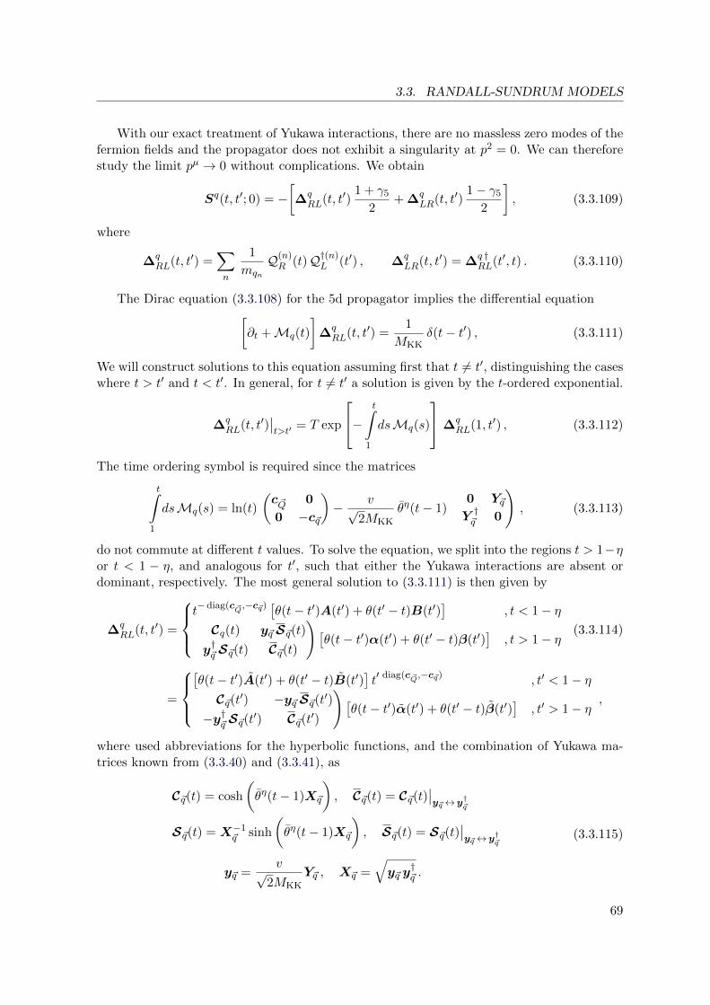
3.3. RANDALL-SUNDRUM MODELS
With our exact treatment of Yukawa interactions, there are no massless zero modes of thefermion fields and the propagator does not exhibit a singularity at p2 = 0. We can thereforestudy the limit pµ → 0 without complications. We obtain
Sq(t, t′; 0) = −[∆qRL(t, t′)
1 + γ5
2+ ∆q
LR(t, t′)1− γ5
2
], (3.3.109)
where
∆qRL(t, t′) =
∑
n
1
mqn
Q(n)R (t)Q†(n)
L (t′) , ∆qLR(t, t′) = ∆q †
RL(t′, t) . (3.3.110)
The Dirac equation (3.3.108) for the 5d propagator implies the differential equation[∂t +Mq(t)
]∆qRL(t, t′) =
1
MKKδ(t− t′) , (3.3.111)
We will construct solutions to this equation assuming first that t 6= t′, distinguishing the caseswhere t > t′ and t < t′. In general, for t 6= t′ a solution is given by the t-ordered exponential.
∆qRL(t, t′)
∣∣t>t′
= T exp
−
t∫
1
dsMq(s)
∆q
RL(1, t′) , (3.3.112)
The time ordering symbol is required since the matrices
t∫
1
dsMq(s) = ln(t)
(c ~Q 0
0 −c~q
)− v√
2MKK
θη(t− 1)
(0 Y~qY †~q 0
), (3.3.113)
do not commute at different t values. To solve the equation, we split into the regions t > 1−ηor t < 1 − η, and analogous for t′, such that either the Yukawa interactions are absent ordominant, respectively. The most general solution to (3.3.111) is then given by
∆qRL(t, t′) =
t− diag(c~Q,−c~q)[θ(t− t′)A(t′) + θ(t′ − t)B(t′)
], t < 1− η(
Cq(t) y~q S~q(t)
y†~q S~q(t) C~q(t)
)[θ(t− t′)α(t′) + θ(t′ − t)β(t′)
], t > 1− η (3.3.114)
=
[θ(t− t′)A(t′) + θ(t′ − t)B(t′)
]t′ diag(c~Q,−c~q) , t′ < 1− η(
C~q(t′) −y~q S~q(t′)
−y†~q S~q(t′) C~q(t′)
)[θ(t− t′)α(t′) + θ(t′ − t)β(t′)
], t′ > 1− η ,
where used abbreviations for the hyperbolic functions, and the combination of Yukawa ma-trices known from (3.3.40) and (3.3.41), as
C~q(t) = cosh
(θη(t− 1)X~q
), C~q(t) = C~q(t)
∣∣y~q↔y†~q
S~q(t) = X−1~q sinh
(θη(t− 1)X~q
), S~q(t) = S~q(t)
∣∣y~q↔y†~q
y~q =v√
2MKK
Y~q , X~q =√y~q y
†~q .
(3.3.115)
69
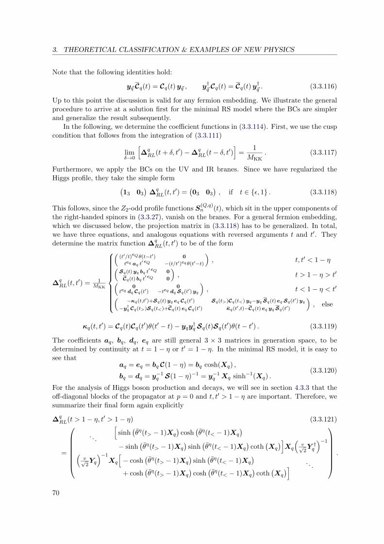
3. THEORETICAL CLASSIFICATION & EXAMPLES OF NEW PHYSICS
Note that the following identities hold:
y~q Cq(t) = Cq(t)y~q , y†~q Cq(t) = Cq(t)y†~q . (3.3.116)
Up to this point the discussion is valid for any fermion embedding. We illustrate the generalprocedure to arrive at a solution first for the minimal RS model where the BCs are simplerand generalize the result subsequently.
In the following, we determine the coefficient functions in (3.3.114). First, we use the cuspcondition that follows from the integration of (3.3.111)
limδ→0
[∆qRL(t+ δ, t′)−∆q
RL(t− δ, t′)]
=1
MKK. (3.3.117)
Furthermore, we apply the BCs on the UV and IR branes. Since we have regularized theHiggs profile, they take the simple form
(13 03
)∆qRL(t, t′) =
(03 03
), if t ∈ ε, 1 . (3.3.118)
This follows, since the Z2-odd profile functions S(Q,q)n (t), which sit in the upper components of
the right-handed spinors in (3.3.27), vanish on the branes. For a general fermion embedding,which we discussed below, the projection matrix in (3.3.118) has to be generalized. In total,we have three equations, and analogous equations with reversed arguments t and t′. Theydetermine the matrix function ∆q
RL(t, t′) to be of the form
∆qRL(t, t′) = 1
MKK
((t′/t)cQθ(t−t′) 0
tcq aq t′ cQ −(t/t′)cq θ(t′−t)
), t, t′ < 1− η
(Sq(t)yq bq t′ cQ 0
Cq(t) bq t′ cQ 0
), t > 1− η > t′
(0 0
tcq dq Cq(t′) −tcq dq Sq(t′)yq
), t < 1− η < t′
( −κq(t,t′)+Sq(t)yq eq Cq(t′) Sq(t>)Cq(t<)yq−yq Sq(t) eq Sq(t′)yq−y†q Cq(t>)Sq(t<)+Cq(t) eq Cq(t′) κq(t′,t)−Cq(t) eq yq Sq(t′)
), else
κq(t, t′) = Cq(t)Cq(t′)θ(t′ − t)− yqy†q Sq(t)Sq(t
′)θ(t− t′) . (3.3.119)
The coefficients aq, bq, dq, eq are still general 3 × 3 matrices in generation space, to bedetermined by continuity at t = 1 − η or t′ = 1 − η. In the minimal RS model, it is easy tosee that
aq = eq = bq C(1− η) = bq cosh(Xq) ,
bq = dq = y−1q S(1− η)−1 = y−1
q Xq sinh−1(Xq) .(3.3.120)
For the analysis of Higgs boson production and decays, we will see in section 4.3.3 that theoff-diagonal blocks of the propagator at p = 0 and t, t′ > 1− η are important. Therefore, wesummarize their final form again explicitly
∆qRL(t > 1− η, t′ > 1− η) (3.3.121)
=
. . .
[sinh
(θη(t> − 1)Xq
)cosh
(θη(t< − 1)Xq
)
− sinh(θη(t> − 1)Xq
)sinh
(θη(t< − 1)Xq
)coth
(Xq
)]Xq
(v√2Y †q)−1
(v√2Yq
)−1Xq
[− cosh
(θη(t> − 1)Xq
)sinh
(θη(t< − 1)Xq
)
+ cosh(θη(t> − 1)Xq
)cosh
(θη(t< − 1)Xq
)coth
(Xq
)]. . .
.
70

3.3. RANDALL-SUNDRUM MODELS
In the following, we generalize the last result by including general 5d fermions with mixedBCs. As explained in section 3.3.5.2, superscripts (+) and (−) indicate Neumann or DirichletBC on the UV brane respectively and even and odd parity is assigned to the two differentchirality projections. We parametrize the number of light fermion generations that emerge
of type Q(+)L and q
(+)R with n+
Q = n+q = nf , and the number of additional partner fermions
Q′ (−)L and q
′ (−)R as n−Q and n−q respectively. We also set nQ,q = nf + n−Q,q and the number of
KK modes per KK level nF = nQ + nq. The additional bulk-mass parameters compared tothe minimal model are called c−Q,q. Remark that Y~q is a complex nQ × nq matrix which wedecompose into its sub-matrices according to the BCs of the fermions, i.e.
y~q =xv√
2Y~q =
(y(++)q y(+−)
q
y(−+)q y(−−)
q
)∈ CnQ×nq . (3.3.122)
The (+,+) sub-block is always of size nf × nf . We start with the general form (3.3.114), usethe cusp condition (3.3.117) and implement the generalized BCs
(1nQ 0nQ×nq
)∆RL(1, t′) = 0nQ×nF , ∆RL(t, 1)
(0nQ×nq
1nq
)= 0nF×nq , (3.3.123)
(1nf 0 0nf 0
0 0n−q ×n−Q0 1n−q
)∆RL(ε, t′) = 0nq×nF , ∆RL(t, ε)
0nf 0
0 1n−Q1nf 0
0 0n−q ×n−Q
= 0nF×nQ .
The general solution reads
∆qRL(t, t′) =
1
MKK× (3.3.124)
×
(t′
t
)cQθ(t− t′) 0 0 0
t−c−Q aq11 t
′ cQ −(t′
t
)c−Qθ(t′ − t) 0 t−c−Q aq12 t
′ −c−q
tcq aq21 t′ cQ 0 −
(tt′
)cqθ(t′ − t) tcq aq22 t′ −c−q
0 0 0(t′
t
)c−q θ(t− t′)
, t, t′ < 1− η
(Sq(t)y~q bq1 t
′ cQ 0nQ×nQ Sq(t)y~q bq2 t′ −c−q
Cq(t) bq1 t′ cQ 0nq×nQ Cq(t) bq2 t′ −c−q
), t > 1− η > t′
0nf×nQ 0nf×nqt−c
−Q dq1 Cq(t′) −t′ −c
−Q dq1 Sq(t
′)yqtcq dq2 Cq(t′) −tcq dq2 Sq(t
′)yq0n−q ×nQ 0n−q ×nq
, t < 1− η < t′
(−κq(t, t′) Sq(t>)Cq(t<)y~q
−y†~q Cq(t>)Sq(t<) κq(t′, t)
)+
(y~q Sq(t)
Cq(t)
)eq
(Cq(t′) − Sq(t
′)y~q), else
71
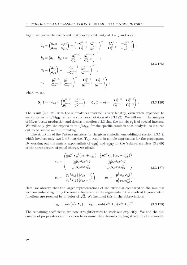
3. THEORETICAL CLASSIFICATION & EXAMPLES OF NEW PHYSICS
Again we derive the coefficient matrices by continuity at 1− η and obtain
aq =
(aq11 aq12
aq21 aq22
)=
(−C(+−)
q ys(++)q
−C(−−)q ys(−+)
q
)−1(C(++)q −ys(+−)
q
C(+−) †q −ys(−−)
q
),
bq =(bq1 bq2
)=
(ys(++)q ys(+−)
q
C(+−) †q C(++)
q
)−1
,
dq =
(dq1dq2
)=
(−C(+−) †
q ys(++)q
−C(−−)q ys(−+)
q
)−1
,
eq =
(ys(++)q ys(+−)
q
C(+−) †q C(−−)
q
)−1(C(++)q C(+−)
q
ys(+−) †q ys(−−) †
q
),
(3.3.125)
where we set
Sq(1− η)y~q =
(ys(++)q ys(+−)
q
ys(−+)q ys(−−)
q
), Cq(1− η) =
(C(++)q C(+−)
q
C(+−) †q C(−−)
q
). (3.3.126)
The result (3.3.125) with the submatrices inserted is very lengthy, even when expanded tosecond order in v/MKK using the sub-block notation of (3.3.122). We will see in the analysisof Higgs boson production and decays in section 4.3.3 that the matrix eq is of special interest.We will only give the expansion in v/MKK for the specific result in that analysis, as it turnsout to be simple and illuminating.
The structure of the Yukawa matrices for the given custodial embedding of section 3.3.5.2,which involves only two 3× 3 matrices Yu,d, results in simple expressions for the propagator.
By working out the matrix exponentials of y~qy†~q and y†~qy~q for the Yukawa matrices (3.3.69)
of the three sectors of equal charge, we obtain
eu =
12y−1u s
−12u
(c2u + c−1
2d
)12y−1u s
−12u
(c2u − c−1
2d
)
1√2y†d s2d c
−12d − 1√
2y†d s2d c
−12d
1√2y†d s2d c
−12d − 1√
2y†d s2d c
−12d
,
ed =
(y−1d s
−12d
(12c2d + 1
)
y−1d s
−12d
(12c2d − 1
)), eλ =
(y†d s2d c
−12d
y†d s2d c−12d
).
(3.3.127)
Here, we observe that the larger representations of the custodial compared to the minimalfermion embedding imply the general feature that the arguments in the involved trigonometricfunctions are rescaled by a factor of
√2. We included this in the abbreviations
c2q = cosh(√
2Xq
), s2q = sinh
(√2Xq
)(√2Xq
)−1. (3.3.128)
The remaining coefficients are now straightforward to work out explicitly. We end the dis-cussion of propagators and move on to examine the relevant coupling structure of the model.
72

3.3. RANDALL-SUNDRUM MODELS
3.3.8 Complete Coupling Structure
In contrast to the discussion of renormalizable, or partly renormalizable models presentedabove, RS models have a conceptually different coupling structure. First of all, the modelsare of course non-renormalizable and therefore loop-order calculations are not expected to beconstrained in their general coupling structure. One has to check process by process if non-UVsensitive statements can be made. Below, we will show the fortunate example of loop processesfor Higgs physics where this is the case. For this purpose, we need a good understanding ofHiggs–fermion couplings, for which we give the relevant results here. Concerning electroweakprecision tests and constraints from FCNC, statements can be made due to the fact that themost relevant processes are influenced already at tree-level. In the following, we will giveall relevant couplings for the case of a minimal as well as the custodial RS model and use anotation that facilitates comparison between them.
3.3.8.1 Higgs–Fermion Couplings
For the derivation of Higgs-boson couplings to fermion currents, we have to compute overlapintegrals of fermion profiles with the δ-profile function of the IR localized Higgs boson. Thecoupling is therefore given by
gRhqmqn =1√2
1∫
ε
dt δη(t− 1)Q†(m)L (t)
(0 Y~qY †~q 0
)Q(n)R (t) . (3.3.129)
The correct procedure is to start from a regularized Higgs profile, insert the profile form(3.3.40), compute the relevant overlap integrals, and then take η to zero [207].
limη→0
gRhqmqn =
√2π
Lε
1∫
ε
dt δη(t− 1)~aQ†m CQm(1− η)
1
cosh2X~q
×[
cosh2(θη(t− 1)X~q
)− sinh2
(θη(t− 1)X~q
) ]Y~qC
qn(1− η)~aqn
=
√2π
Lε~aQ†m CQ
m(1−)1
cosh2X~q
Y~qCqn(1−)~aqn .
(3.3.130)
In this equation there is of course the implicit assumption that the fermion mass xqn is fixed,while the limit on η is performed. It is useful to consider the expression also for finite η andvery large KK masses. One can derive that the form of the couplings changes drastically inthe region xqn ≈Mweak/η. We illustrate this behavior in a simple toy model with one fermiongeneration and vanishing bulk masses in appendix A.3. Here, we only summarize that thequalitative difference in the case of one generation is that inside a given KK level the two KKfermions of that level show a diagonal Higgs-boson coupling of opposite sign if xqn Mweak/η.Close to the threshold Mweak/η, one of the couplings vanishes approximately, while the otherstays finite.
Remark that (3.3.130) involves a combination of Yukawa matrices that is different fromY~q defined in (3.3.41), which determines the spectrum. This has relevant consequences for theflavor off-diagonal transitions, which receive a contribution that is not chirally suppressed,i.e. not proportional to one of the external quark masses.
73
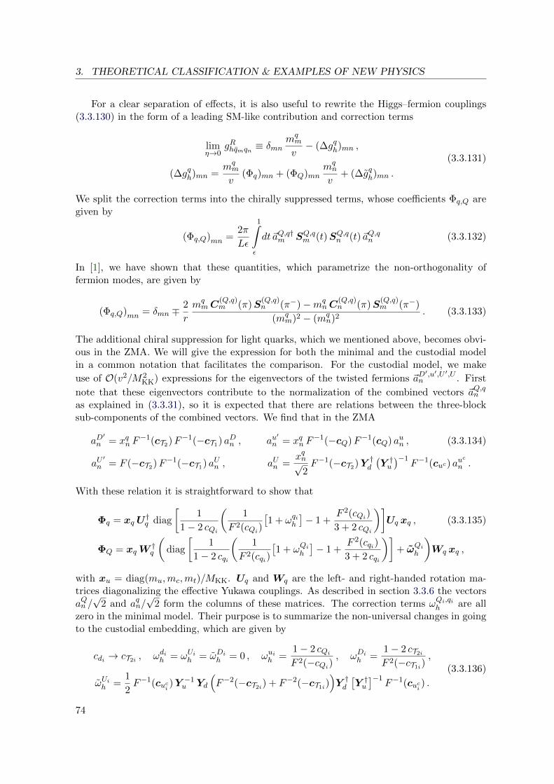
3. THEORETICAL CLASSIFICATION & EXAMPLES OF NEW PHYSICS
For a clear separation of effects, it is also useful to rewrite the Higgs–fermion couplings(3.3.130) in the form of a leading SM-like contribution and correction terms
limη→0
gRhqmqn ≡ δmnmqm
v− (∆gqh)mn ,
(∆gqh)mn =mqm
v(Φq)mn + (ΦQ)mn
mqn
v+ (∆gqh)mn .
(3.3.131)
We split the correction terms into the chirally suppressed terms, whose coefficients Φq,Q aregiven by
(Φq,Q)mn =2π
Lε
1∫
ε
dt~aQ,q†m SQ,qm (t)SQ,qn (t)~aQ,qn (3.3.132)
In [1], we have shown that these quantities, which parametrize the non-orthogonality offermion modes, are given by
(Φq,Q)mn = δmn ∓2
r
mqmC
(Q,q)m (π)S
(Q,q)n (π−)−mq
nC(Q,q)n (π)S
(Q,q)m (π−)
(mqm)2 − (mq
n)2. (3.3.133)
The additional chiral suppression for light quarks, which we mentioned above, becomes obvi-ous in the ZMA. We will give the expression for both the minimal and the custodial modelin a common notation that facilitates the comparison. For the custodial model, we make
use of O(v2/M2KK) expressions for the eigenvectors of the twisted fermions ~aD
′,u′,U ′,Un . First
note that these eigenvectors contribute to the normalization of the combined vectors ~aQ,qn
as explained in (3.3.31), so it is expected that there are relations between the three-blocksub-components of the combined vectors. We find that in the ZMA
aD′
n = xqn F−1(cT2)F−1(−cT1) aDn , au
′n = xqn F
−1(−cQ)F−1(cQ) aun , (3.3.134)
aU′
n = F (−cT2)F−1(−cT1) aUn , aUn =xqn√
2F−1(−cT2)Y †d
(Y †u)−1
F−1(cuc) auc
n .
With these relation it is straightforward to show that
Φq = xqU†q diag
[1
1− 2 cQi
(1
F 2(cQi)
[1 + ωqih
]− 1 +
F 2(cQi)
3 + 2 cQi
)]Uq xq , (3.3.135)
ΦQ = xqW†q
(diag
[1
1− 2 cqi
(1
F 2(cqi)
[1 + ωQih
]− 1 +
F 2(cqi)
3 + 2 cqi
)]+ ωQih
)Wq xq ,
with xu = diag(mu,mc,mt)/MKK. Uq and Wq are the left- and right-handed rotation ma-trices diagonalizing the effective Yukawa couplings. As described in section 3.3.6 the vectorsaQn /√
2 and aqn/√
2 form the columns of these matrices. The correction terms ωQi,qih are allzero in the minimal model. Their purpose is to summarize the non-universal changes in goingto the custodial embedding, which are given by
cdi → cT2i , ωdih = ωUih = ωDih = 0 , ωuih =1− 2 cQiF 2(−cQi)
, ωDih =1− 2 cT2iF 2(−cT1i)
,
ωUih =1
2F−1(cuci )Y
−1u Yd
(F−2(−cT2i) + F−2(−cT1i)
)Y †d[Y †u]−1
F−1(cuci ) .
(3.3.136)
74
3.3. RANDALL-SUNDRUM MODELS
The correction terms involve the zero-mode profiles F (−cT1i), F (−cT2i), and F (−cQi), which
arise from the admixture of the ST1(−)n (t), S
T2(−)n (t), and S
Q(−)n (t) profiles in the corresponding
zero-mode profile. In each case, the suppression by v/MKK due to the admixture is offsetby the O(MKK/v) enhancement of the Z2-odd (−) profile relative to its (+) counterpart.For cQi < 1/2, the leading contribution in Φu is thus numerically enhanced by a factor of
approximately 2 with respect to the minimal model. If the ZdiLdjL vertices are protected from
fermion mixing by cT1 = cT2 and cT2i < 1/2, then the same holds true for ΦD. Depending onthe structure of the Yukawa matrices and bulk masses, also an enhancement in ΦU is possible.
The second type of corrections to the Higgs–fermion couplings (3.3.131) is given by
∆gqh = −√
22π
Lε
1∫
ε
dt δ(t− 1)(~a q †m S q
m(t)Y †~q SQn (t)~aQn
)mn
=
√2v2
3M2KK
π
Lε
(~aQ †m CQ
m(1−) Y~q Y†~q Y~q C
qn(1−)~a qn
)mn
,
(3.3.137)
with
Y †~q ≡ Y†~q
3
2
[X−2q + atanh
(Xq
)X−1q
(1− X−2
q
)]. (3.3.138)
The result in the ZMA becomes simply
∆gqh =v2
3√
2M2KK
U †q F (cQi)Yq Y†q Yq F (cqi)Wq ·
1 , minimal RS,
2 , custodial RS.(3.3.139)
Notice that this kind of correction is not parametrically suppressed by light quark massesfor the first two up and all down type generations. The chirally unsuppressed contributions∆gd,uh arise from the Z2-odd Yukawa couplings, and present the dominant sources of flavorviolation in the Higgs sector [207]. They are potentially comparable to Z boson mediated
FCNCs. Compared to the minimal RS model, the corrections ∆gd,uh are again bigger by afactor of 2 in the extended scenario.
Note that for the diagonal entries we can write the ZMA result (3.3.139) also as
(∆gqh)nn =4m2
t
3vM2KK
3∑
j=1
mqj
(U †q F
−2(cQ)Uu
)jn
(W †
u F−2(cq)Wu
)nj·
12
. (3.3.140)
The term with j = n is obviously positive semi-definite. Since terms with j = 1, 2 have achiral suppression compared to the term with j = 3, we find that (∆guh)33 is real and positiveto a good approximation, while the phase of all other entries of (∆guh)nn can take in principleany value. Since also (∆ΦQ,q)nn are absolute squares, we conclude with the important resultthat htt and hbb couplings are predicted to be suppressed relative to their SM values in all RSmodels discussed here. A similar conclusion has been drawn in the context of models wherethe Higgs arises as a pseudo Nambu-Goldstone boson [236, 237].
Let us finally mention that a model-independent analysis of the flavor misalignment of theSM fermion masses and the Yukawa couplings has been presented in [238]. There, it has beenshown that at the level of dimension six, chirally unsuppressed contributions to flavor-changingHiggs boson vertices will generically arise from dimension 6 operators like q iL Φ qjR (Φ†Φ) inmodels where the Higgs boson is a bound state of a new strongly interacting theory. If
75

3. THEORETICAL CLASSIFICATION & EXAMPLES OF NEW PHYSICS
present, the latter terms will dominate over the chirally suppressed contributions originatingfrom operators of the form q iL /Dq
jL (Φ†Φ). This is due to the possibly large couplings yq∗ of the
composite Higgs boson to the other strongly interacting states, which results in y2q∗/(16π2)
mq/v. Considering all relevant dimension-six operators in the given RS models to lowestorder of the mass insertion approximation, allows to recover the ZMA results (3.3.135) and(3.3.139) quantifying the misalignment between the Yukawa couplings and the zero-modemasses (see [207] for a illuminating discussion). We emphasize that our exact solution givenabove resums all new-physics effects induced by the mass insertions, corresponding to boththe non-derivative and derivative dimension-six operators. The interplay of both in fact leadsto the chirally unsuppressed terms in (3.3.131).
3.3.8.2 Gauge-Boson–Fermion Couplings
We turn to the phenomenologically relevant expressions for weak gauge interactions of quarkcurrents and identify the RS contribution at order v2/M2
KK. For the Z-boson couplings toquarks, we extract a universal prefactor and write the couplings in (infinite-dimensional)matrix form as
gσZqmqn =g
cw
[1 +
M2Z
4M2KK
(1− 1
L
)](gqZ,σ
)mn
, (3.3.141)
with
gqZ,L =(T 3 qLL − s2
wQq)[
1− M2Z
2M2KK
(ωqLZ L∆Q −∆′Q
)]− δQ +
M2Z
2M2KK
(L εQ − ε′Q
),
gqZ,R = −s2wQq
[1− M2
Z
2M2KK
(ωqRZ L∆q −∆′q
)]+ δq −
M2Z
2M2KK
(L εq − ε′q
). (3.3.142)
The charges are either SM-like for the minimal RS model, or as summarized in table 3.4 forthe custodial RS model. For the latter, we define T 3 qL
σ for σ = L,R as the quantum numbersof the quark in the uppermost component of ~Q and T 3 qR
σ via the uppermost component of ~qin the notation of (3.3.23). Like in the case of Higgs-fermion couplings there is an embeddingdependent factor in the leading contribution, which comes linear in L ≈ 34. Analogous tobefore, we encode this in a factor ωqZ . However, here the factor is universal for all generations.It is given by ωqZ in the minimal RS model and for a general LR-symmetric embedding as
ωqZ = 1− sZcZ
gZ′ QqZ ′
gZ QqZ
=c2w
2g2L
(g2L + g2
R)(T 3 qL + T 3 q
R ) + (g2L − g2
R)(T 3 qL − T
3 qR )
T 3 qL − s2
wQq. (3.3.143)
This allows one to read off that the two possible choices
PC symmetry: T 3 qL = T 3 q
R = 0 ,
PLR symmetry: gL = gR , T 3 qL = −T 3 q
R ,(3.3.144)
are suitable to protect the Z-boson vertices from receiving L-enhanced corrections. Since thecustodial representation (3.3.66) features T 3 dL
L = −T 3 dLR , T 3λL
L = −T 3λLR and T 3uR
L,R = 0, we
observe that the ZdiLdjL, ZλiLλ
jL, and ZuiRu
jR vertices are protected to leading order in L by
the PLR and PC symmetries, respectively. On the other hand, the L-enhanced corrections
76

3.3. RANDALL-SUNDRUM MODELS
of the vertices with opposite fermion chiralities are raised by ωdRZ ≈ 10.0, ωλRZ ≈ 2.0, andωuLZ ≈ 2.2.
In (3.3.142), we have furthermore split the corrections to the Z-boson couplings into
leading contributions, denoted by ∆(′)Q,q, and subleading ones, parametrized by ε
(′)Q,q. The
elements of the leading contributions are defined as
(∆Q
)mn(
∆′Q)mn
=
2π
Lε
1∫
ε
dt
t2
t2(
12 − ln(t)
) [
~aQ†m CQm(t)CQ
n (t)~aQn + ~a q†m Sqm(t)Sqn(t)~a qn
],
(3.3.145)
and the same formulas with Q↔ q. In the minimal model, the subleading contributions ε(′)Q,q
are obtained from the same equations without the contribution from the even profiles CQ,qm .
Furthermore, the matrices δQ,q, which arise from of the non-orthonormality of the quark pro-files and describe mixings between the different multiplets, are given by the same expressionsΦQ,q that were defined in (3.3.132). They inherently contain a O(v2/M2
KK) suppression andare formally of the same order as the ∆Q,q, for which this suppression is factored out in(3.3.142). Employing the ZMA and neglecting O(1) factors, one can show that all the leading
quantities (∆(′)Q,q)ij and (δQ,q)ij have an inherent suppression with two factors of the profile
brane values F (cQi,qi)F (cQj ,qj ) of the corresponding fermions [1]. Light mass values and thesmallness of non-standard contributions to gauge-boson couplings are therefore correlated.This is the RS-GIM mechanism [201, 202]. In the custodial model, the general order of mag-nitude of the expressions is unchanged, however the expression become more involved. Wesummarize
• minimal :
ε(′)Q,q = T 3 q
L ∆(′)Q,q
∣∣CQ,qn →0
, δQ,q = T 3 qL ΦQ,q . (3.3.146)
• custodial :
(εQ)mn(
ε′Q)mn
=
2π
Lε
1∫
ε
dt
c2wt
2
t2(
12 − ln(t)
)× (3.3.147)
×[~aQ†m CQ
m(t)(T 3 qLL 1− T 3Q
L +t2W0
(T 3 qLR 1− T 3Q
R
))CQn (t)~aQn
+ ~a q†m Sqm(t)
(T 3 qLL 1− T 3 q
L +t2W0
(T 3 qLR 1− T 3 q
R
))Sqn(t)~a qn
],
(εq)mn(
ε′q)mn
=
2π
Lε
1∫
ε
dt
c2wt
2
t2(
12 − ln(t)
)×
×[~a q†m C
qm(t)
(T 3 qL −
t2W0
(T 3 qRR 1− T 3 q
R
))Cqn(t)~a qn
+ ~aQ†m SQm(t)(T 3QL −
t2W0
(T 3 qRR 1− T 3Q
R
))SQn (t)~aQn
],
(δQ)mn
=2π
Lε
1∫
ε
dt[~aQ†m CQ
m(t)(T 3 qLL 1− T 3Q
L
)CQn (t)~aQn (3.3.148)
+ ~a q†m Sqm(t)
(T 3 qLL 1− T 3 q
L
)Sqn(t)~a qn
],
77
3. THEORETICAL CLASSIFICATION & EXAMPLES OF NEW PHYSICS
(δq)mn
=2π
Lε
1∫
ε
dt[~a q†m C
qm(t)T 3 q
L Cqn(t)~a qn + ~aQ†m SQm(t)T 3Q
L S Qn (t)~aQn
].
In the expressions above, we abbreviated the diagonal charge matrices as T 3Q,qσ=L,R :
T 3Uσ = diag
(T 3uσ 1nf , T
3u′σ 1nf
), T 3u
σ = diag(T 3uc
σ 1nf , T3U ′σ 1nf , T
3Uσ 1nf
),
T 3Dσ = T 3 d
σ 1nf , T 3 dσ = diag
(T 3Dσ 1nf , T
3D′σ 1nf
), (3.3.149)
T 3 Λσ = T 3λ
σ 1nf , T 3λσ = diag
(T 3 Λ′σ 1nf , T
3 Λσ 1nf
).
Note that with the embedding (3.3.66), the matrices T 3uσ vanish identically. ZMA results
have been given in [1] and [4] and we do not repeat them here, except for one case below.The second ingredient for the protection of the ZbiLb
jL vertex in the custodial model can
now be derived from (3.3.148). Inserting quantum numbers we see that18
δD = −1
2
2π
Lε
1∫
ε
dt(aD†m ST2(+)
m (t)ST2(+)n (t) aDn − aD
′†m ST1(−)
m (t)ST1(−)n (t) aD
′n
)mn
= −1
2xdW
†d diag
[1
1− 2cT2i
(1
F 2(cT2i)
[1− ωqih
]− 1 +
F 2(cT2i)3 + 2cT2i
)]Wd xd ,
(3.3.150)
where the second line in the approximation in the ZMA. The quantity ωqih has been defined in(3.3.136). In fact it enters ΦD in (3.3.135) with the opposite sign. The rest of the expressionis unchanged compared to (3.3.150). We have seen there that ωqih is one to a very goodapproximation if cT1i = cT2i < 1/2. The equality of bulk masses is of course enforced by thePLR symmetry acting on the down-type quarks as PLR(D′) = D. In consequence, effects dueto quark mixing entering the Z-boson couplings are generically suppressed in the custodialRS model relative to the minimal scenario as long as the Z2-odd quark fields are not too farlocalized in the UV. It remains a viable option to break this symmetry softly by choosingdifferent bulk masses, since the zero mode masses are not affected by cT1i in an appreciableway, as long as they stay UV localized. The protection mechanism discussed here has alsobeen studied in [239] employing a perturbative approach to electroweak symmetry breaking.Compared to the perturbative approach, the exact treatment of the EOMs used here has thesalient advantage that the dependence of the ZdiLd
jL vertices on quark mixing, i.e. on the
bulk masses MT1,2 in (3.3.150), can be clearly deciphered.
It is interesting to observe that only the leading terms in L and F−2(cT2) of the ZdiLdjL
vertex can be protected. There is no such mechanism available for the subleading terms, sincethey arise from the fact that the twisted and untwisted orbifold representations obey differentUV BCs. These effects hence represent an irreducible source of PLR symmetry breaking.
3.3.8.3 Purely Bosonic Couplings
Finally, we will also evaluate the RS corrections to the W+W−h, ZZh, and W+W−Z tree-level vertices, where the gauge bosons are the SM-like zero-modes. They will be important forour discussion of Higgs processes. Due to the unbroken U(1)EM gauge group, the W+W−γ
18The second line of (3.3.150) also holds in the minimal model with cT2i → cdi and ωqih = 0.
78
3.3. RANDALL-SUNDRUM MODELS
coupling is unchanged with respect to the SM to all orders in v2/M2KK. Furthermore, the
calculation of the W+W−Z vertex is greatly simplified by the following two observations.First, one has
2π
L
1∫
ε
dt
tχ
(+)0 (t) =
√2π +O
(v4
M4KK
), (3.3.151)
and second(( ~Aa0)2 χ
(−)0 (t)
)2= O(v4/M4
KK). In combination, these two relations imply thatthe W+W−Z vertex does not receive corrections at O(v2/M2
KK) in the RS model, regardless ofthe specific gauge group. By the same line of reasoning, it is also readily seen that all quarticgauge-boson vertices first differ at order v4/M4
KK from the corresponding SM expressions.We express the W+W−h, ZZh vertices relative to their SM expressions. To expand the
zero-mode profiles in M2V /M
2KK we use (3.3.80) evaluated at the IR brane and (3.3.82). We
obtain
κV =gV V ∗h|RS
gV V ∗h|SM= 1− M2
V
M2KK
(L
c2V
− 1 +1
2L
)+O
(v4
M4KK
). (3.3.152)
In the case of the PLR symmetry in the custodial model, one has c−2W = 2 and c−2
Z = 2 c2w,
which implies that the leading absolute correction to gW+W−h and gW+W−h takes the form−2M2
V /M2KK L. For MKK = 2 TeV (MKK = 3 TeV) these terms lead to a suppression of
the WWh and ZZh couplings by about −10% (−5%) compared to the SM. In the minimalRS model, expression (3.3.152) holds with cV → 1, and consequently the corrections to thecouplings of the Higgs boson to massive gauge bosons are smaller by about a factor of 2. Ourfinding that the couplings WWh and ZZh experience a reduction from their SM expectationsconfirms the model-independent statements made in [237].
3.3.8.4 Four Fermion Couplings
It this final section on the fundamentals of the RS coupling structure, we discuss four-fermioninteractions induced by the exchange of the 5d propagator at low momentum using the resultsof section 3.3.7. The resulting effective Hamiltonian encodes the effects obtained by integrat-ing out all new physics and is valid below the matching scale µKK = O(MKK). We start withthe case of charged currents with leptons and quarks. They are relevant for the extraction ofthe CKM matrix. Again, we extract a universal prefactor of the Wilson coefficients
H(W )eff =
2πα
s2wM
2W
[1 +
M2W
4M2KK
(1− 1
L
)]∑
l
[uLγ
µVL dL + uRγµVR dR
](lLγµνl L) + h.c. .
(3.3.153)The total prefactor defines the modified expression of GF , as we discuss in section 4.2.2. TheCKM matrices as extracted from experiment are given by
VL = ∆+Q +√
2 ε+ q − M2W
2M2KK
L(∆+Q +
√2 ε+ q
),
VR =√
2 ∆+ q + ε+Q − M2W
2M2KK
L(√
2 ∆+ q + ε+Q),
(3.3.154)
with ∆+Q,qmn
∆+Q,qmn
=
2π
Lε
1∫
ε
dt ~aU,u†m CU,um (t)
ΩQ,q
t2 ΩQ,q
CD,dn (t)~aD,dn , (3.3.155)
79

3. THEORETICAL CLASSIFICATION & EXAMPLES OF NEW PHYSICS
and ε+Q,qmn , ε+Q,q
mn defined by analogous formulas with the even profiles CQ,qi replaced by odd
profiles SQ,qi . The involved kernel-matrices are given by ΩQ = ΩQ = 1 and Ωq = Ωq = 0 inthe minimal RS model, and
ΩQ =
(1
0
), Ωq =
0 00 10 0
, ΩQ =
1
−g2R
g2L
1
, Ωq =
0 00 1
−g2R
g2L
1 0
,
(3.3.156)in the model with custodial protection.
Notice that this definition of VL,R includes the exchange of the entire tower of W bosonsand their KK excitations and therefore differs from the definition of the CKM matrix employedin [1, 239], which is based on the WuiLd
jL and WuiRd
jR vertices.
Of particular interest for the discussion of constraints from FCNCs in section 4.1.2 arethe effective dimension six operators arising from the tree-level exchange of KK photons andgluons and of Z bosons. Again, the relevant sums over KK modes are evaluated with thetechniques presented in section 3.3.7. In the case of KK-photon exchange, we find that theeffective Hamiltonian is given by
H(γ)eff =
2πα
M2KK
∑
f,f ′
Qf Qf ′
1
2L
(fγµf
)(f ′γµf ′
)− 2(fLγ
µ∆′F fL + fRγµ∆′ffR
)(f ′γµf ′
)
+ 2L(fLγ
µ∆F fL + fRγµ∆ffR
)⊗(f ′Lγµ∆F ′f
′L + f ′Rγµ∆f ′f
′R
). (3.3.157)
The matrices ∆′A have been defined in (3.3.145). In addition, we encounter non-factorizableoverlap integrals that are the relevant sources of ∆F = 2 transitions
(∆F
)mn⊗(∆f ′)m′n′
=2π2
L2ε2
1∫
ε
dt
1∫
ε
dt′ t2< (3.3.158)
×[~a(F )†m C(Q)
m (φ)C(Q)n (φ)~a(F )
n + ~a(f)†m S(f)
m (φ)S(f)n (φ)~a(f)
n
]
×[~a
(f ′)†m′ C
(f ′)m′ (φ′)C(f ′)
n′ (φ′)~a(f ′)n′ + ~a
(F ′)†m′ S
(Q)m′ (φ′)S(Q)
n′ (φ′)~a(F ′)n′
].
The result (3.3.157) is exact, i.e. no expansion in powers of v2/M2KK has been performed.
The effective interactions arising from KK-gluon exchange have an analogous structure. Weonly need to restrict the sum over fermions in (3.3.157) to quarks and replace αQf Qf ′ byαs T
a ⊗ T a, where the color matrices ta must be inserted inside the quark bilinears. Theexpressions for the flavor matrices defined in (3.3.158) are tensor products, which a priori donot factorize in the form of simple matrix products. In the ZMA, we obtain [229]
(∆F
)mn⊗(∆f ′)m′n′≈∑
i,j
(U †f)mi
(Uf)in
(∆Ff )ij(W †f)m′j
(Wf
)jn′,
(∆Ff )ij =F 2(cFi)
3 + 2cFi
3 + cFi + cfj2(2 + cFi + cfj )
F 2(cfj )
3 + 2cfj.
(3.3.159)
Analogous expressions hold for the remaining combinations of indices F and f . Using thefact that all ci parameters except cu3 are very close to −1/2, it is a reasonable approximation
80

3.3. RANDALL-SUNDRUM MODELS
to replace (3 + cFi + cfj )/(2 + cFi + cfj ) by 2, in which case we obtain rough approximation
∆A ⊗ ∆B ≈∆A ∆B , (3.3.160)
In the same approximation, there is no need to distinguish between the ∆′A and ∆A matrices.We found that this approximate factorization receives significant corrections in setups wherethe volume of the extra dimension in reduced to L . 10 [229], and (3.3.159) obtains relevantsubleading contributions if the down-type singlet bulk masses cdi are aligned [3]. We discussthese cases closer in section 4.1.2.
The interactions arising from the exchange of the Z boson and its KK excitations have aricher structure. We have given the full and exact effective Hamiltonian in [1]. Here, we onlyrepeat the contributions at O(v2/M2
KK) which renders the result compact
H(Z)eff =
4πα
s2wc
2wm
2Z
[1 +
m2Z
2M2KK
(1− 1
2L
)]JµZ JZµ (3.3.161)
− 8πα
s2wc
2wm
2Z
∑
f
[fLγ
µT f3 δF fL − fRγµT f3 δffR]JZµ
− 4παL
s2wc
2wM
2KK
∑
f
ωfZ
[ (T f3 − s2
wQf
)fLγ
µ∆F fL − s2wQf fRγ
µ∆ffR
]JZµ
+4παL
s2wc
2wM
2KK
∑
f,f ′
Ωf f ′
Z
[ (T f3 − s2
wQf
)fLγ
µ∆F fL − s2wQf fRγ
µ∆ffR
]
⊗[ (T f′
3 − s2wQf ′
)f ′Lγµ∆F ′f
′L − s2
wQf ′ f′Rγµ∆f ′f
′R
].
Here, JµZ is the familiar SM expression for the neutral current
JµZ ≡∑
f
[(T f3 − s2
wQf)fLγ
µfL − s2wQf fRγ
µfR
]. (3.3.162)
The differences between the minimal and custodial RS model are again encoded in the fac-tors ωfZ as defined in (3.3.143) and another universal factor for the non-factorizable overlapintegrals given by
Ωff ′
Z = 1 +g2Z′ Q
fZ′ Q
f ′
Z′
g2Z Q
fZ Q
f ′
Z
= 1 +c2w
(1− ωfZ
)(1− ωf ′Z
)
1−(
1 +g2L
g2R
)s2w
. (3.3.163)
In order to abbreviate the notation in (3.3.161), the factors ωfZ and Ωff ′
Z are meant to actas operators on the fermion bilinears in the sense that f and f ′ depend on the chiralities ofthe corresponding fermions. Remark the reversed sign in (3.3.163) and the absent factor ofsZ/cZ compared to (3.3.143), which directly come from the corresponding factors of the t2<and t2 terms in (3.3.102). The numerical values
ΩdLdLZ = 2.5 , ΩdLdR
Z = −10.9 , ΩdRdRZ = 94.6 , (3.3.164)
are necessary to explain differences in down type ∆F = 2 FCNCs in the different fermionembeddings. To this end, one needs of course to compare the overall size of the Z-bosonand KK-gluon contributions to the latter processes. We will review this more closely insection 4.1.2.
81

82
Chapter 4
Aspects of Precision Physics
4.1 Flavor Physics
It is well known that precision flavor observables put strong constraints on generic new physics.In most models, the constraints are complementary to bounds derived from collider searchesfor direct production of resonances and to astrophysical bounds. This is due to the inherentdependence of flavor off-diagonal observables on the Yukawa sector and its deviations fromthe SM prediction. Hence, while models of new physics typically predict new particles, whoseexistence will be scrutinized by LHC experiments, it is important to examine their effects onprecision flavor observables as well, in order to check the consistency of the models.
The objective of our discussion is twofold. First, we shall study amplitudes necessary forflavor physics on a conceptual level for any theory with perturbatively unitary high energybehavior. Secondly, we shall also present a numerical analysis of bounds and correlationsfrom flavor observables in a specific example that does not fall into the latter class, the RSmodel.
In the conceptual part, our intention can be summarized as follows: A repeatedly emergingtask is the calculation of amplitudes for fermion transitions between different generations,induced by a massive neutral gauge boson at one-loop — the so-called penguin amplitude.An example is the FCNC s → d transition with the emission of a virtual Z boson, leadingto processes like the rare K → πνν decays. Just like the SM, many models of new physicsgenerate this transition first at the one-loop level. This property drastically improves thepotential agreement of a model with experimental flavor constraints, especially from ∆S = 2observables. In the absence of a tree-level coupling for this process, we expect UV-finitenessof the penguin amplitude. However, the practical verification in models with many new gaugeand Goldstone bosons in a renormalizable gauge can be tedious. We perform this calculationfor any spontaneously broken gauge theory, using the generic Lagrangian supplemented withthe implied STIs as presented in section 3.1. We demonstrate and advocate the practicaluse of the STIs to perform renormalization and simplifications of this generic process. Wegive the full template result for the finite Z penguin and also for box-type diagrams, therebyspecializing to down-type quarks for notational convenience. Yet, the result can also beapplied to up-type and lepton-flavor-violating processes. The generic result is useful, sincethe flavor amplitudes for any model of new physics can now be quickly implemented by
83

4. ASPECTS OF PRECISION PHYSICS
the simple specification of its couplings of physical particles.1 We check that the full resultindeed reproduces the well known SM-result and the result of the LHT model introducedin section 3.2. For the latter model we provide a deeper understanding why the Z penguinturns out be free of UV-sensitivity and investigate whether this is due to the partly gaugedstructure of the model. As a byproduct, we also simplify the result for the Z penguin andboxes considerably as compared to the literature.
In the numerical analysis, we study the bounds and correlations in the RS model. Wefocus on kaon mixing and direct CP violation in K → ππ, since measurements of theseprocesses provide the strongest bounds on the scale of the model. The RS model possessestree-level FCNCs but explains the smallness of the corresponding observables by the RS-GIM mechanism (see section 3.3.8.2). It is well known that this suppression is typicallyinsufficient to explain the smallness of observed FCNCs. We find that the dependence on theYukawa sector introduces a significant spread in the distribution of the RS predictions. Wequantitatively assess the implications on the scale bounds and find a strong dependence, evenin the case of non-fine-tuned RS scenarios. The bounds inferred from flavor processes thusdepend strongly on the required amount of viable parameter space. We derive new boundsfrom the lower edge of these distributions, which are more robust than the typical boundsoften quoted in the literature. This makes the scale bounds more comparable to bounds fromelectroweak precision observables. We also discuss two scenarios that are specifically designedto alleviate the flavor bounds, a model with active flavor-symmetry SU(3)d for singlet down-type quarks and a model with a reduced volume of the extra dimension.
Beyond the scale bounds, we find that the restriction of the Yukawa structure also leadsto complementary predictions, i.e. correlations between different flavor observables. To thisend, we study leptonic and semileptonic kaon decays. The phenomenological discussion isrounded off with a discussion of CKM non-unitarity and predictions for the rare B decaysinto two muons, where measurements recently start to probe the RS parameter space.
4.1.1 Structure of ∆F = 1 Processes in Perturbative Models
4.1.1.1 Renormalization of the Generic Z Penguin
In the following we present the derivation of the generic result for the Z penguin. To thisend the renormalization by using the STIs of section 3.1.2 is described in some detail. Wegive the results in (4.1.9) – (4.1.10). It is self-contained and can be used as it stands. Thereader who is interested in the result only might skip this discussion, which serves to clarifythe structure of the result and shows how our method can be extended to include tree-leveldj → di transitions.
Generally, in order to determine the Wilson coefficients of an effective theory, it is sufficientto match the effective actions in both the full and the effective theory. This entails thatwe have to compute one-light-particle irreducible diagrams only. In particular, diagramswith self-energy insertions on external light particle legs should not be included. However,in certain models containing tree-level transitions between down-type quarks of the samegeneration, diagrams with a heavy particle reducible line exist on the full theory side of thematching. Typically, this reducible line might be due to a down-type vector-like fermion.
1 A potential application is to link the template to the output of a computer algebra package such asFeynRules [240], creating an automated yet simple tool for the generation of analytic flavor results withoutthe need to invoke a full amplitude generator.
84

4.1. FLAVOR PHYSICS
An example of this is found in models where the flavor symmetry SU(3)3 is considerednon-accidental and gauged [241, 242], thereby extending the idea of minimal flavor violation(MFV) and explaining quark-hierarchies with a see-saw mechanism. This concept receivedrenewed interest in the last years as a consequence of the persistent failure to find new physicsin flavor violating transitions. Since the flavor group is anomalous, new heavy fermions haveto be added to the theory. Another example are effective models that extend the SM by avector-like fermionic sector in order to explain the hierarchy of SM Yukawa couplings throughsmall mixing angles between the SM and heavy fermions [56, 243, 244]. Such a setup canbe used to effectively parametrize the fermionic contributions that arise in the RS model ofsection 3.3, where these effects are, however, subleading in all relevant cases. Furthermore,such models generically induce flavor-violating Z couplings to light quarks, which we excludefrom the discussion here.
The fermion one-loop self-energies in the full theory lead to mixing among the fermionsbeyond tree level. We perform an off-diagonal field renormalization for both heavy and lightfermions, with finite terms chosen to restore diagonal and canonically normalized kineticand mass terms [245]. In consequence, diagrams of the form shown in figure 4.1 are exactlycanceled by corresponding counterterm diagrams. However, we have to carefully treat the
Z
d′dj di Figure 4.1: One-heavy-particlereducible contribution to the Zpenguin.
renormalization constants that the self-energy sub-diagram in figure 4.1 induces in the vertexrenormalization.
We first calculate the one-loop corrections to the renormalized fermion two-point function.They can be written as
δΓfjfiσ =
[(Σψ,σ
V,fifj+ δZψ,σ
H,fifj
)/p+ Σψ,σ
S,fifj− 1
2
(mfiδZ
ψ,σ
fifj+ δZψ,σ †
fifjmfj
)− δijδmfi
]Pσ , (4.1.1)
where the fermion-field-renormalization constant is written as a sum of a Hermitian and ananti-Hermitian part. δmfi is an additive mass renormalization. The divergent parts of theHermitian field-renormalization constants have the simple structure
δZψ,σH,fifj
∣∣div≡ 1
2
(δZψ,σ
fifj+ δZψ,σ †
fifj
)∣∣div
= −Σψ,σ
V,fifj
∣∣div
= − ∆
16π2
[1
2
∑s′,f ′
yσs′fif ′ yσs′f ′fj
(4.1.2)
+∑v′,f ′
gσv′fif ′ g
σv′f ′fj
+m2f ′
2m2v′
(gσv′fif ′ −
mfimf ′
gσv′fif ′
)(gσv′f ′fj −
mfjmf ′
gσv′f ′fj
)].
Here ∆ = 1/ε− γE + ln(4π) includes also the finite MS subtractions, d = 4− 2ε is the space-time dimension in dimensional regularization, and γE is Euler’s constant. The finite parts ofthe field-renormalization constants for i 6= j are given by
δZψ,σfifj
∣∣fin
=1
m2fi−m2
fj
(m2fj
Σψ,σ
V,fifj+mfimfjΣ
ψ,σ
V,fifj+mfiΣ
ψ,σ
S,fifj+mfjΣ
ψ,σ
S,fifj
)∣∣fin, (4.1.3)
δZψ,σ †fifj
∣∣fin
= − 1
m2fi−m2
fj
(m2fi
Σψ,σ
V,fifj+mfimfjΣ
ψ,σ
V,fifj+mfiΣ
ψ,σ
S,fifj+mfjΣ
ψ,σ
S,fifj
)∣∣fin.
85

4. ASPECTS OF PRECISION PHYSICS
They enter our generic result after having been expanded in small mass ratios. The diagonalfield-renormalization constants are not necessary in our case. For a full generalization to tree-level dj → di transitions, or an analogous treatment of charged current couplings, one wouldhave to fix these constants by renormalization conditions. The best practice here depends onthe context and we will not go into further details. As a non-trivial example we mention therenormalization of the SM CKM matrix in non-minimal schemes that preserve decoupling,where it turns out that STIs allow to renormalize the CKM-matrix gauge-independently butrestrict the diagonal field renormalization constants [246].
In the following section we present the general result for models (or parts thereof) wheretree-level FCNCs for the dj → di transition are absent; in this case the contributions ofthe vertex and gauge-boson field-renormalization constants vanish. Here, we will show thatall divergences in our generic result completely cancel against the divergent terms in thefield rotation, without the necessity of additional counterterms. This is due to the absenceof tree-level contributions to the Z penguin, to which these counterterms would be propor-tional. In order to make this cancellation manifest, it is necessary to use the consequencesof tree-level perturbative unitarity derived in section 3.1.1 in form of the STIs. They yieldrelations between various couplings, and allow for the automatic inclusion of the effects ofthe would-be Goldstone bosons. This step is independent of the specification of a model andcan be applied without detailed knowledge about the sector responsible for the spontaneoussymmetry breaking. Note that the following treatment is valid also in the general case ofnon-flavor-diagonal tree-level couplings.
We are now ready to study the general expression for the one-loop contributions to therenormalized Vvaψfjψfk three-point function. They are given by
δΓfjfivaµσ = Γ
fjfiva,(1)µσ +
[δZg,σ
vafifj+
1
2
∑f ′
(gσvafif ′ δZ
ψ,σ
f ′fj+ δZψ,σ †
fif ′gσvaf ′fj
)
+1
2
∑v′δZVvav′ g
σv′fifj
]Pσ .
(4.1.4)
Here, Γvafjfi,(1)µσ denotes the sum of all contributing one-loop diagrams, and the rest are
the vertex, fermion field, and gauge-boson field-renormalization constants, respectively. Weuse the STIs (3.1.19), (3.1.28) and (3.1.29) to show that the fermion-field-renormalizationconstants are sufficient to cancel all divergences in (4.1.4). In principle, the procedure isstraightforward. It is instructive to start with considering the divergence of the diagram thatcontains three internal particles of different spin, one scalar s′, one fermion f ′, and one vectorv′, and is thus proportional to the couplings gvav′s′ g
σv′fjf ′
gσs′f ′fi
. It turns out that the sum
over all such possible diagrams can be rewritten by using (3.1.28) and (3.1.29). In figure 4.2we illustrate how the sum rules have to be combined with couplings, which are separated bythe dotted cut line, in order to match the divergence of one of the mixed diagrams. Aftersubtracting the sum of these two contributions from the total divergence and inserting theexplicit expressions of the fermion-field-renormalization constants (4.1.2), the reformulatedexpression can be grouped into parts that involve either internal scalars or internal vectors.In fact, the contributions with two internal scalars are already finite now. The remainingcontributions are treated analogously. E.g. from the diagram with two internal vectors, weinfer that (3.1.19) must be combined with gvav′v′′ and summed over v′ and v′′ in order toreformulate the remaining part of the divergence with two internal vectors. Finally, the
86
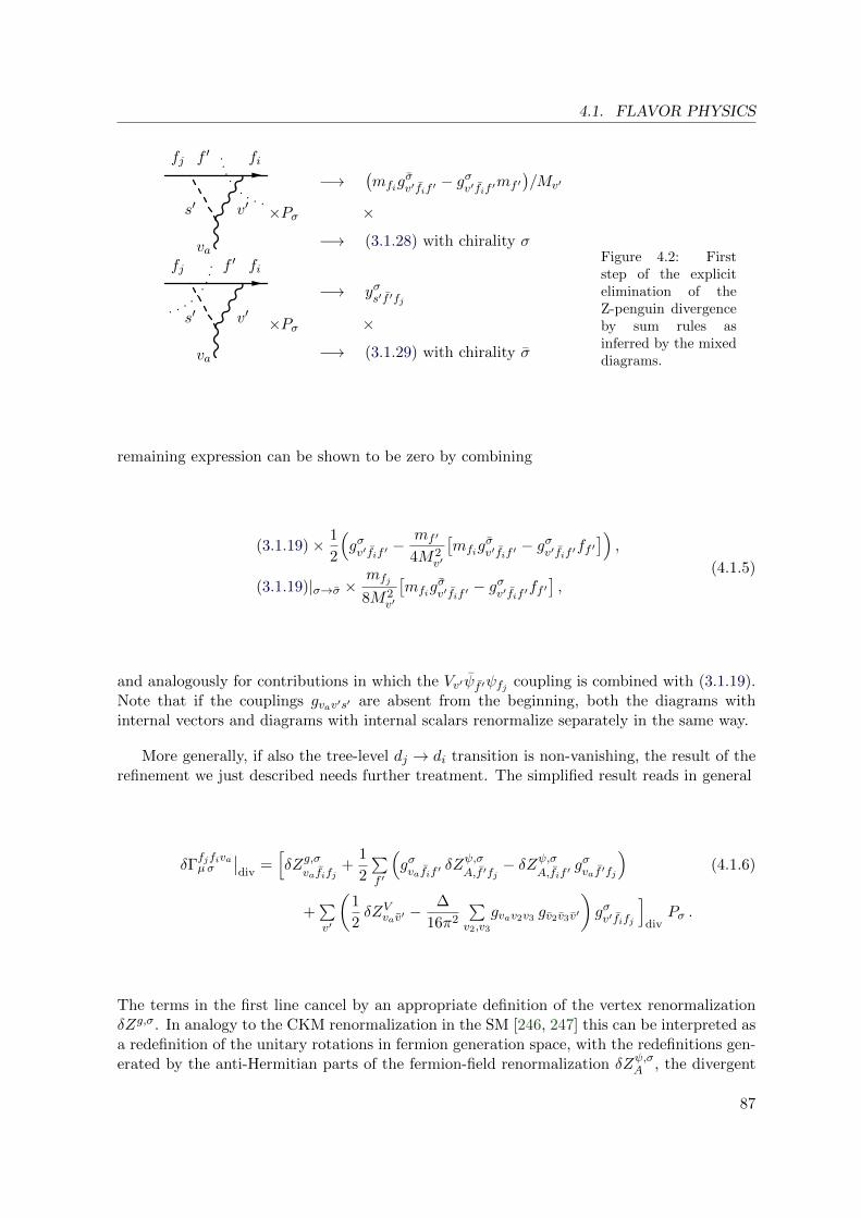
4.1. FLAVOR PHYSICS
fj fi
s′ v′
va
f ′
fj fi
s′ v′
va
f ′
−→(mfig
σv′fif ′
− gσv′fif ′mf ′)/Mv′
×Pσ ×−→ (3.1.28) with chirality σ
−→ yσs′f ′fj
×Pσ ×−→ (3.1.29) with chirality σ
Figure 4.2: Firststep of the explicitelimination of theZ-penguin divergenceby sum rules asinferred by the mixeddiagrams.
remaining expression can be shown to be zero by combining
(3.1.19)× 1
2
(gσv′fif ′ −
mf ′
4M2v′
[mfig
σv′fif ′
− gσv′fif ′ff ′]),
(3.1.19)|σ→σ ×mfj
8M2v′
[mfig
σv′fif ′
− gσv′fif ′ff ′],
(4.1.5)
and analogously for contributions in which the Vv′ψf ′ψfj coupling is combined with (3.1.19).Note that if the couplings gvav′s′ are absent from the beginning, both the diagrams withinternal vectors and diagrams with internal scalars renormalize separately in the same way.
More generally, if also the tree-level dj → di transition is non-vanishing, the result of therefinement we just described needs further treatment. The simplified result reads in general
δΓfjfivaµσ
∣∣div
=[δZg,σ
vafifj+
1
2
∑f ′
(gσvafif ′ δZ
ψ,σ
A,f ′fj− δZψ,σ
A,fif ′gσvaf ′fj
)(4.1.6)
+∑v′
(1
2δZVvav′ −
∆
16π2
∑v2,v3
gvav2v3 gv2v3v′
)gσv′fifj
]div
Pσ .
The terms in the first line cancel by an appropriate definition of the vertex renormalizationδZg,σ. In analogy to the CKM renormalization in the SM [246, 247] this can be interpreted asa redefinition of the unitary rotations in fermion generation space, with the redefinitions gen-erated by the anti-Hermitian parts of the fermion-field renormalization δZψ,σA , the divergent
87

4. ASPECTS OF PRECISION PHYSICS
parts of which read explicitly
δZψ,σA,fifj
=
12mfi
[Σψ,σ
S,fifi− Σψ,σ
S,fifi
]div
, j = k
2m2fi−m2
fj
[m2fi
+m2fj
2 Σψ,σ
V,fifj+mfimfjΣ
ψ,σ
V,fifj+mfiΣ
ψ,σ
S,fifj+ Σψ,σ
S,fifjmfj
]div, j 6= k
=∆
16π2
( ∑s′,f ′
1−δij
m2fi−m2
fj
(m2fi
+m2fj
2 yσs′fif ′yσs′f ′fj
+mfimfj yσs′fif ′
yσs′f ′fj
+ 2mf ′
(mfi y
σs′fif ′
yσs′f ′fj +mfj yσs′fif ′
yσs′f ′fj
))
+ δijmf ′2mfi
(yσs′fif ′y
σs′f ′i − yσs′fif ′y
σs′f ′fi
)(4.1.7)
+∑v′,f ′
1−δij
m2fi−m2
fj
(gσv′fif ′g
σv′f ′fj
((m2
fi+m2
fj)(
1− 3m2f ′
2m2v′
)+
m2fim2fj
m2v′
)
+ gσv′fif ′gσv′f ′fj
mfimfj
(2 +
m2fi
+m2fj−6m2
f ′
2m2v′
)
+ gσv′fif ′gσv′f ′fj
mf ′mfj
(− 8 +
m2fi−m2
fj+4m2
f ′
2m2v′
)
+ gσv′fif ′gσv′f ′fj
mfimf ′
(− 8 +
m2fj−m2
fi+4m2
f ′
2m2v′
))
+ δijmf ′mfi
(2 +
m2fi−m2
f ′
2m2v′
)(gσv′fif ′g
σv′f ′fi
− gσv′fif ′gσv′f ′di
)).
The terms in the second line of (4.1.6) vanish after an explicit Z-boson field renormalization.To see this, one would have to use the STIs for ghost couplings and additional sum ruleswhich we included in the appendix (see (A.1.2)). In fact, one can read off the result for theZ-boson field renormalization from the fact that the second line in (4.1.6) has to vanish. Thefinite part of the renormalization will lead to a shift which is universal for all flavors and canbe absorbed in the corresponding gauge-coupling constant.
4.1.1.2 Result for the Generic Z Penguin and Box Diagrams
We present our result for the renormalized Z penguin in the form of an effective vertex, inthe spirit of [248]. The penguin function CσdjdiZ is defined in terms of the amputated vertexfunction as
ΓdjdiZµσ = γµPσ
GF√2
e
π2M2Z
cwswCσdjdiZ , (4.1.8)
and depends on all masses which appear. σ = L,R stands for the chiral projection. Settingthe external momenta and light fermion masses to zero in our results, we obtain in the
88
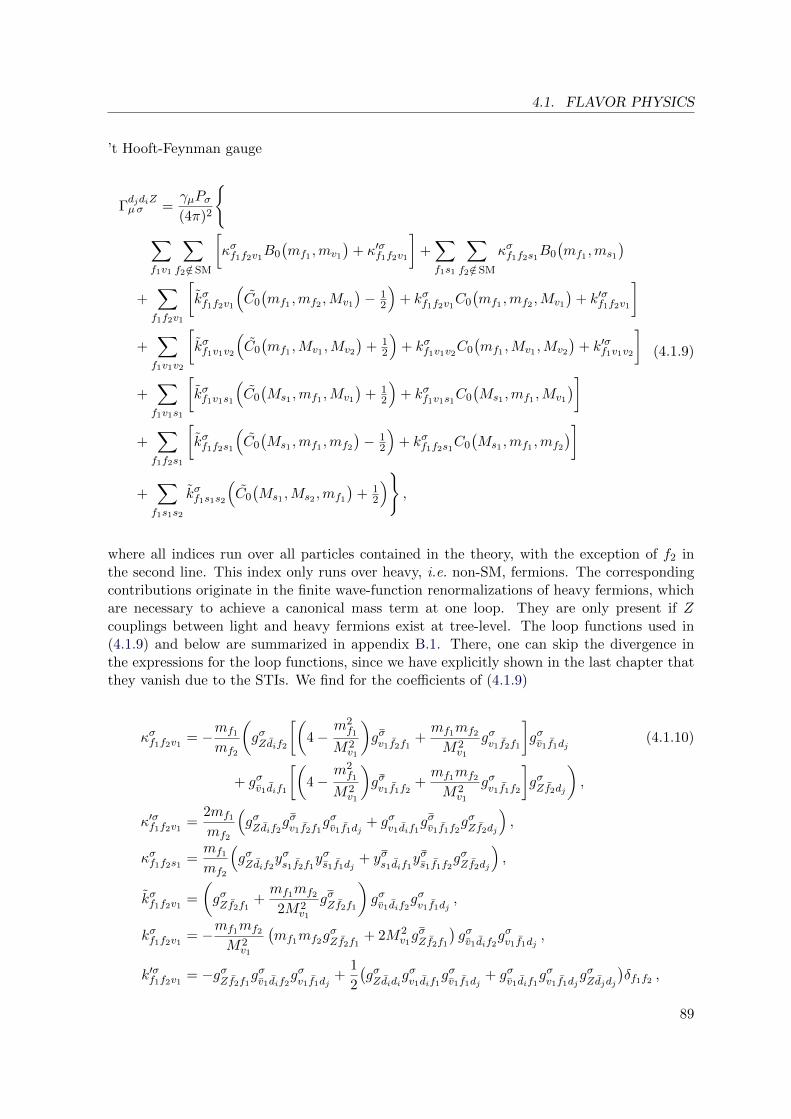
4.1. FLAVOR PHYSICS
’t Hooft-Feynman gauge
ΓdjdiZµσ =
γµPσ(4π)2
∑
f1v1
∑
f2 /∈ SM
[κσf1f2v1
B0
(mf1 ,mv1
)+ κ′σf1f2v1
]+∑
f1s1
∑
f2 /∈ SM
κσf1f2s1B0
(mf1 ,ms1
)
+∑
f1f2v1
[kσf1f2v1
(C0
(mf1 ,mf2 ,Mv1
)− 1
2
)+ kσf1f2v1
C0
(mf1 ,mf2 ,Mv1
)+ k′σf1f2v1
]
+∑
f1v1v2
[kσf1v1v2
(C0
(mf1 ,Mv1 ,Mv2
)+ 1
2
)+ kσf1v1v2
C0
(mf1 ,Mv1 ,Mv2
)+ k′σf1v1v2
]
+∑
f1v1s1
[kσf1v1s1
(C0
(Ms1 ,mf1 ,Mv1
)+ 1
2
)+ kσf1v1s1C0
(Ms1 ,mf1 ,Mv1
)]
+∑
f1f2s1
[kσf1f2s1
(C0
(Ms1 ,mf1 ,mf2
)− 1
2
)+ kσf1f2s1C0
(Ms1 ,mf1 ,mf2
)]
+∑
f1s1s2
kσf1s1s2
(C0
(Ms1 ,Ms2 ,mf1
)+ 1
2
),
(4.1.9)
where all indices run over all particles contained in the theory, with the exception of f2 inthe second line. This index only runs over heavy, i.e. non-SM, fermions. The correspondingcontributions originate in the finite wave-function renormalizations of heavy fermions, whichare necessary to achieve a canonical mass term at one loop. They are only present if Zcouplings between light and heavy fermions exist at tree-level. The loop functions used in(4.1.9) and below are summarized in appendix B.1. There, one can skip the divergence inthe expressions for the loop functions, since we have explicitly shown in the last chapter thatthey vanish due to the STIs. We find for the coefficients of (4.1.9)
κσf1f2v1= −mf1
mf2
(gσZdif2
[(4−
m2f1
M2v1
)gσv1f2f1
+mf1mf2
M2v1
gσv1f2f1
]gσv1f1dj
(4.1.10)
+ gσv1dif1
[(4−
m2f1
M2v1
)gσv1f1f2
+mf1mf2
M2v1
gσv1f1f2
]gσZf2dj
),
κ′σf1f2v1=
2mf1
mf2
(gσZdif2
gσv1f2f1gσv1f1dj
+ gσv1dif1gσv1f1f2
gσZf2dj
),
κσf1f2s1 =mf1
mf2
(gσZdif2
yσs1f2f1yσs1f1dj
+ yσs1dif1yσs1f1f2
gσZf2dj
),
kσf1f2v1=
(gσZf2f1
+mf1mf2
2M2v1
gσZf2f1
)gσv1dif2
gσv1f1dj,
kσf1f2v1= −mf1mf2
M2v1
(mf1mf2g
σZf2f1
+ 2M2v1gσZf2f1
)gσv1dif2
gσv1f1dj,
k′σf1f2v1= −gσZf2f1
gσv1dif2gσv1f1dj
+1
2
(gσZdidig
σv1dif1
gσv1f1dj+ gσv1dif1
gσv1f1djgσZdjdj
)δf1f2 ,
89
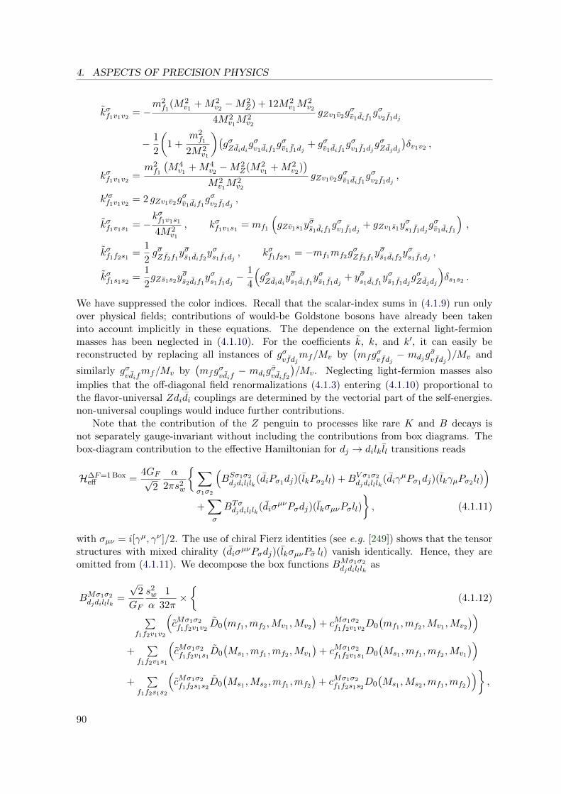
4. ASPECTS OF PRECISION PHYSICS
kσf1v1v2= −
m2f1
(M2v1
+M2v2−M2
Z) + 12M2v1M2v2
4M2v1M2v2
gZv1v2gσv1dif1
gσv2f1dj
− 1
2
(1 +
m2f1
2M2v1
)(gσZdidig
σv1dif1
gσv1f1dj+ gσv1dif1
gσv1f1djgσZdjdj
)δv1v2 ,
kσf1v1v2=m2f1
(M4v1
+M4v2−M2
Z(M2v1
+M2v2
))
M2v1M2v2
gZv1v2gσv1dif1
gσv2f1dj,
k′σf1v1v2= 2 gZv1v2g
σv1dif1
gσv2f1dj,
kσf1v1s1 = −kσf1v1s1
4M2v1
, kσf1v1s1 = mf1
(gZv1s1y
σs1dif1
gσv1f1dj+ gZv1s1y
σs1f1dj
gσv1dif1
),
kσf1f2s1 =1
2gσZf2f1
yσs1dif2yσs1f1dj
, kσf1f2s1 = −mf1mf2gσZf2f1
yσs1dif2yσs1f1dj
,
kσf1s1s2 =1
2gZs1s2y
σs2dif1
yσs1f1dj− 1
4
(gσZdidiy
σs1dif1
yσs1f1dj+ yσs1dif1
yσs1f1djgσZdjdj
)δs1s2 .
We have suppressed the color indices. Recall that the scalar-index sums in (4.1.9) run onlyover physical fields; contributions of would-be Goldstone bosons have already been takeninto account implicitly in these equations. The dependence on the external light-fermionmasses has been neglected in (4.1.10). For the coefficients k, k, and k′, it can easily bereconstructed by replacing all instances of gσ
vfdjmf/Mv by
(mfg
σvfdj− mdjg
σvfdj
)/Mv and
similarly gσvdif
mf/Mv by(mfg
σvdif− mdig
σvdif2
)/Mv. Neglecting light-fermion masses also
implies that the off-diagonal field renormalizations (4.1.3) entering (4.1.10) proportional tothe flavor-universal Zdidi couplings are determined by the vectorial part of the self-energies.non-universal couplings would induce further contributions.
Note that the contribution of the Z penguin to processes like rare K and B decays isnot separately gauge-invariant without including the contributions from box diagrams. Thebox-diagram contribution to the effective Hamiltonian for dj → dilk ll transitions reads
H∆F=1 Boxeff =
4GF√2
α
2πs2w
∑
σ1σ2
(BSσ1σ2djdilllk
(diPσ1dj)(lkPσ2 ll) +BV σ1σ2djdilllk
(diγµPσ1dj)(lkγµPσ2 ll)
)
+∑
σ
BTσdjdilllk
(diσµνPσdj)(lkσµνPσll)
, (4.1.11)
with σµν = i[γµ, γν ]/2. The use of chiral Fierz identities (see e.g. [249]) shows that the tensorstructures with mixed chirality (diσ
µνPσdj)(lkσµνPσ ll) vanish identically. Hence, they areomitted from (4.1.11). We decompose the box functions BMσ1σ2
djdilllkas
BMσ1σ2djdilllk
=
√2
GF
s2w
α
1
32π×
(4.1.12)
∑f1f2v1v2
(cMσ1σ2f1f2v1v2
D0
(mf1 ,mf2 ,Mv1 ,Mv2
)+ cMσ1σ2
f1f2v1v2D0
(mf1 ,mf2 ,Mv1 ,Mv2
))
+∑
f1f2v1s1
(cMσ1σ2f1f2v1s1
D0
(Ms1 ,mf1 ,mf2 ,Mv1
)+ cMσ1σ2
f1f2v1s1D0
(Ms1 ,mf1 ,mf2 ,Mv1
))
+∑
f1f2s1s2
(cMσ1σ2f1f2s1s2
D0
(Ms1 ,Ms2 ,mf1 ,mf2
)+ cMσ1σ2
f1f2s1s2D0
(Ms1 ,Ms2 ,mf1 ,mf2
)),
90
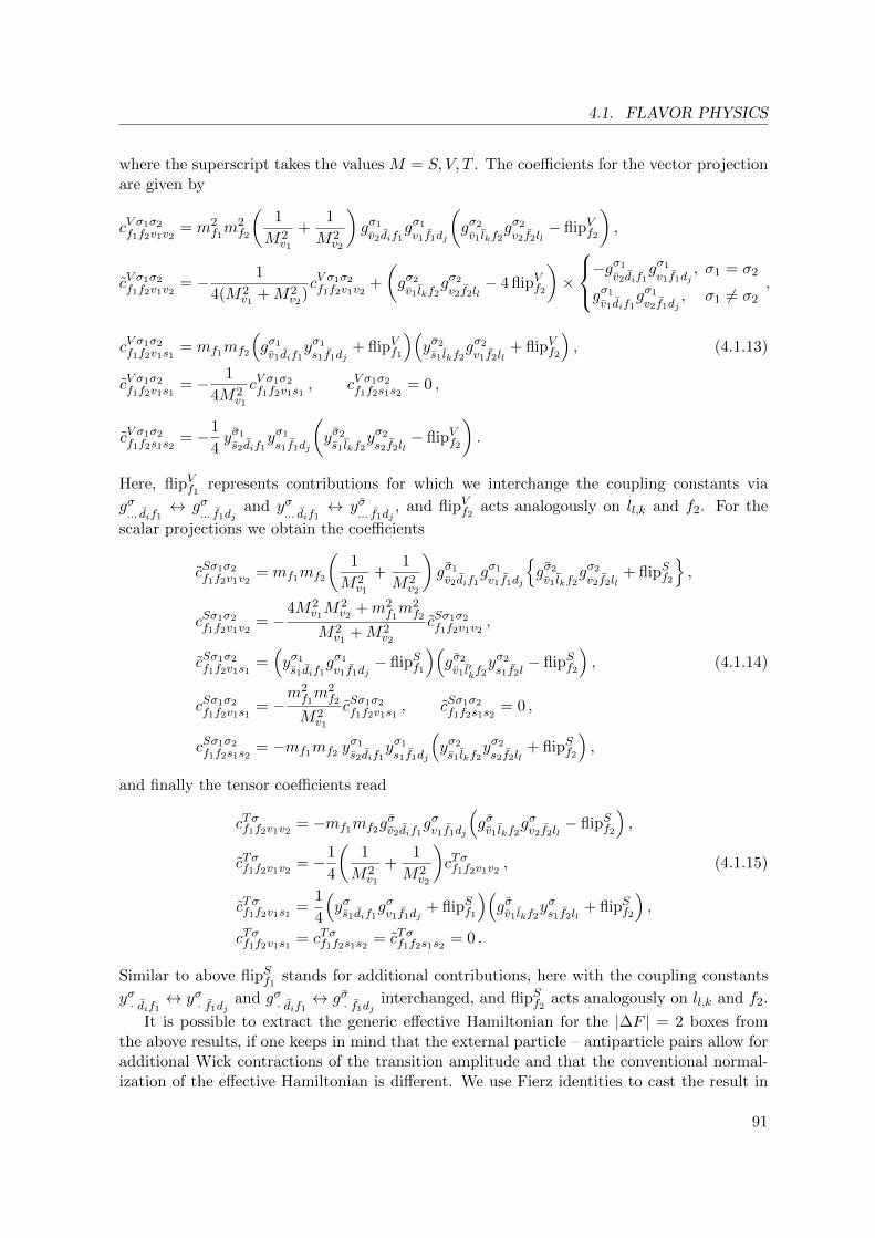
4.1. FLAVOR PHYSICS
where the superscript takes the values M = S, V, T . The coefficients for the vector projectionare given by
cV σ1σ2f1f2v1v2
= m2f1m2f2
(1
M2v1
+1
M2v2
)gσ1
v2dif1gσ1
v1f1dj
(gσ2
v1 lkf2gσ2
v2f2ll− flipVf2
),
cV σ1σ2f1f2v1v2
= − 1
4(M2v1
+M2v2
)cV σ1σ2f1f2v1v2
+
(gσ2
v1 lkf2gσ2
v2f2ll− 4 flipVf2
)×
−gσ1
v2dif1gσ1
v1f1dj, σ1 = σ2
gσ1
v1dif1gσ1
v2f1dj, σ1 6= σ2
,
cV σ1σ2f1f2v1s1
= mf1mf2
(gσ1
v1dif1yσ1
s1f1dj+ flipVf1
)(yσ2
s1 lkf2gσ2
v1f2ll+ flipVf2
), (4.1.13)
cV σ1σ2f1f2v1s1
= − 1
4M2v1
cV σ1σ2f1f2v1s1
, cV σ1σ2f1f2s1s2
= 0 ,
cV σ1σ2f1f2s1s2
= −1
4yσ1
s2dif1yσ1
s1f1dj
(yσ2
s1 lkf2yσ2
s2f2ll− flipVf2
).
Here, flipVf1represents contributions for which we interchange the coupling constants via
gσ... dif1
↔ gσ... f1dj
and yσ... dif1
↔ yσ... f1dj
, and flipVf2acts analogously on ll,k and f2. For the
scalar projections we obtain the coefficients
cSσ1σ2f1f2v1v2
= mf1mf2
(1
M2v1
+1
M2v2
)gσ1
v2dif1gσ1
v1f1dj
gσ2
v1 lkf2gσ2
v2f2ll+ flipSf2
,
cSσ1σ2f1f2v1v2
= −4M2
v1M2v2
+m2f1m2f2
M2v1
+M2v2
cSσ1σ2f1f2v1v2
,
cSσ1σ2f1f2v1s1
=(yσ1
s1dif1gσ1
v1f1dj− flipSf1
)(gσ2
v1 l′kf2yσ2
s1f2l− flipSf2
), (4.1.14)
cSσ1σ2f1f2v1s1
= −m2f1m2f2
M2v1
cSσ1σ2f1f2v1s1
, cSσ1σ2f1f2s1s2
= 0 ,
cSσ1σ2f1f2s1s2
= −mf1mf2 yσ1
s2dif1yσ1
s1f1dj
(yσ2
s1 lkf2yσ2
s2f2ll+ flipSf2
),
and finally the tensor coefficients read
cTσf1f2v1v2= −mf1mf2g
σv2dif1
gσv1f1dj
(gσv1 lkf2
gσv2f2ll− flipSf2
),
cTσf1f2v1v2= −1
4
(1
M2v1
+1
M2v2
)cTσf1f2v1v2
, (4.1.15)
cTσf1f2v1s1 =1
4
(yσs1dif1
gσv1f1dj+ flipSf1
)(gσv1 lkf2
yσs1f2ll+ flipSf2
),
cTσf1f2v1s1 = cTσf1f2s1s2 = cTσf1f2s1s2 = 0 .
Similar to above flipSf1stands for additional contributions, here with the coupling constants
yσ· dif1↔ yσ· f1dj
and gσ· dif1↔ gσ· f1dj
interchanged, and flipSf2acts analogously on ll,k and f2.
It is possible to extract the generic effective Hamiltonian for the |∆F | = 2 boxes fromthe above results, if one keeps in mind that the external particle – antiparticle pairs allow foradditional Wick contractions of the transition amplitude and that the conventional normal-ization of the effective Hamiltonian is different. We use Fierz identities to cast the result in
91

4. ASPECTS OF PRECISION PHYSICS
the operator basis of [250] where
H∆F=2 Boxeff =
G2F
4π2M2W
(∑
σ
SV σσ1,djdiQV σσ1,didj
+∑
n=1,2
(SLRn,djdi Q
LRn,didj
+∑
σ
SSσσn,djdiQSσσn,didj
)),
QV σσ1 = (djγµPσdi)(djγµPσdi) ,
QLR1 = (djγµPLdi)(djγµPRdi) , QLR2 = (djPLdi)(djPRdi) ,
QSσσ1 = (djPσdi)(djPσdi) , QSσσ2 = (dαj Pσdβi )(dβj Pσd
αi ) .
(4.1.16)
A summation over color indices α, β is understood. In order to obtain the coefficients S from(4.1.13)–(4.1.15), the following prescription holds:
SV σσ1,djdi= 4BV σσ
djdilllk|lk,l→ di,j ,
SLR1,djdi= 8BV LR
djdilllk|lk,l→ di,j , SRL1,djdi
= 8BSLRdjdilllk
|lk,l→ di,j ,
SSσσ1,djdi=(4BSσσ
djdilllk− 16BTσσ
djdilllk
)|lk,l→ di,j , SSσσ1,djdi
= −32BTσσdjdilllk
|lk,l→ di,j .
(4.1.17)
As a check of the normalization and general structure of the result, we insert the SM cou-plings in (4.1.9) and (4.1.10). All necessary couplings were already mentioned in section 3.1.2.As usual, we set xq ≡ m2
q/M2W and rewrite the loop-functions in terms of xuk and M2
W . Termsindependent of xuk drop in the result due to the CKM unitarity. This is the well known GIMmechanism [16]. We recover the result of Inami and Lim [251]
CL (SM)djdiZ
= λ(djdi)t C(xt) , C(x) =
x
8
(x− 6
x− 1+
3x+ 2
(x− 1)2ln(x)
), (4.1.18)
for the top-quark contribution to the dj → diZ vertex. The relevant CKM-factors are abbre-
viated as λ(djdi)q = VqdjV
∗qdi
. Similarly we recover from (4.1.12) the result of the box diagrams
for the vertices dj → di e+e− and dj → di ν ν
BV LL (SM)djdiee
= −1
4BV LL (SM)djdiνν
= λ(d′d)t B(xt) , B(x) =
x
4
(1
1− x +ln(x)
(x− 1)2
), (4.1.19)
and for the ∆F = 2 transition dj → di djdi
SV LL (SM)djdidjdi
=(λ
(djdi)t
)2S(xt) +
(λ
(djdi)c
)2S(xc) + 2λ
(djdi)t λ
(djdi)c S(xc, xt) , (4.1.20)
S(x) = S(x, x) , S(x, y) =xS′(y)− yS′(x)
x− y ,
S′(x) = −x4
(3
x− 1+
4− 8x+ x2
(x− 1)2ln(x)
).
Here we kept the finite contribution from the charm-quark mass mc, which is important dueto the CKM factor Re(λc) = O(λ), whereas λt = O(λ5) = Im(λc). The unusual definition ofS in terms of S′ turns out to be useful for the result in the LHT model, which we give in thefollowing section.
92

4.1. FLAVOR PHYSICS
4.1.1.3 Results for the Littlest Higgs Model with T -parity
In the following we apply our results to the partly renormalizable LHT model of section 3.2.This provides the insight why the Z penguin is UV finite in the given model. As a byproduct,we reproduce the result in the literature and simplify it considerably.
We obtain the analytic expressions for quark-flavor violating Z penguin and box diagrams,by inserting the couplings of appendix A.2 into the generic results (4.1.9), (4.1.12), and(4.1.17). Using this specified expression, we can check if the divergence of the penguin diagramvanishes. We find that this is indeed the case. It is only expected on general grounds, ifthe sum rules (3.1.19), (3.1.28), and (3.1.29) hold in all possible combinations of externalparticles that can appear in the penguin diagram after applying the cuts demonstrated insection 4.1.1.1. In other words, if we can verify that the relevant parts entering the process inquestion all fulfill the constraints from tree-level perturbativity, we are allowed to safely use(4.1.9) also for models with sectors of explicitly broken symmetry. This is the case for thepartly gauged LHT model. We created all possible combinations of tree-subdiagrams for theoff-diagonal down-type Z penguin and found that the STIs (3.1.19) are indeed fulfilled. TheSTIs (3.1.28) and (3.1.29) are not exactly fulfilled for subdiagrams with an external down-type mirror-quark. However, the difference of left- and right-hand side of these STIs is alwayssuppressed with a light quark mass mdi or mdj
2. Furthermore, the differences are proportional
to the mirror-mixing matrix VHd (or V †Hd). The remaining coupling, necessary to form the
penguin diagram always contributes another factor of V †Hd (or VHd). After a summation overthe “cut” particle line, the unitarity of VHd implies that even the differences proportional tothe light quark masses mdi,j vanish in the penguin diagram3. It is interesting to note thateven though the complete divergence in the down-type Z penguin vanishes identically, thereare parts of the divergence (proportional to light quark masses), which do not vanish dueperturbative unitarity, but only accidentally. This provides a deeper understanding why theZ penguin turns out be free of UV-sensitivity in the LHT model.
We also reproduce the finite part for the Z penguin and box diagrams as known in theliterature [160, 163, 165, 253]. We summarize it here in a shorter form. To this end we define
xT = m2T+/m
2W , zk = mu 2
H,k/m2WH
, yn = mν 2H,n/m
2WH
,
λq =(V)qdj
(V)∗qdi, ξk =
(VHd
)kdj
(VHd
)∗kdi
, λHln =(VHl)nll
(VHl)∗nlk
,(4.1.21)
and arrive at the result
CL (LHT)djdiZ
=v2
4f2
λt
x2L
2V 2tb
(− 5− xt
[1− 2xL1− xL
+ 2 ln(xt)
]+ (3 + 2xt) ln(xT )
)(4.1.22)
+∑
k=2,3
ξk[C(zk)− C(z1)
],
2The quark-mass suppression comes in addition to the v2/f2 suppression of the new physics contributionto the penguin diagram. Hence, the terms are only conceptually interesting.
3There are similar mb terms in the relevant subdiagrams for the calculation of Z → bb. Only a fullcalculation can show if these contributions also vanish accidentally. Neglecting the mb terms, the finiteness ofthe Z → bb amplitude has been explicitly confirmed in [252]
93
4. ASPECTS OF PRECISION PHYSICS
BV LL (LHT)djdilllk
=v2
4f2
3± 5
2λtx2L
V 2tb
δl′l (4.1.23)
± 1
16
3∑
n=1
∑
k=2,3
λHln ξk
[B′±(zk, yn)−B′±(z1, yn) +B′±(zk)−B′±(z1)
],
SV LL (LHT)1,djdi
=v2
4f2
λtx2L
V 2tb
(λt
xt xL1− xL
+∑
q=c,t
λq
[8S′(xq) + 2xq ln(xT )
])(4.1.24)
− 1
4
∑
j,k=2,3
ξj ξk
[B′−(zj , zk)−B′−(zj , z1)−B′−(z1, zk) +B′−(z1, z1)
].
In (4.1.23) the upper (lower) sign is valid for l = ν (l = e). The second row of each equationcontains the contribution originating from T -odd particles. There, we also used the GIMmechanism for the matrix VHd, which generates the subtracted terms with z1. For the T -oddbox contributions we introduced the following additional loop functions
B′±(z, y) =−(3± 9)zy
(z − 1)(y − 1)+
z(z3 − 8z2 + (10± 9)z − 6 t2w
25 (z − 1))
(z − 1)2(z − y)ln(z) + . . . |z→y
,
B′±(z) = z
(10± 9
z − 1+ (z − 8)
z ln(z)
(z − 1)2
). (4.1.25)
Remark that the results given here completely reproduce the full results of [160, 253], but wesummarized it in a much shorter form. This is achieved by using the vertex definition of theCKM-matrix V given in (3.2.29). This renders the input parameters also closer to physicalobservables. Furthermore, we have expanded in the mass ratio m2
AH/m2
ZH= t2w (1−v2/f2)/5.
In the latter ratio we neglect higher order terms; they are of the same numerical size that oneexpects from the likewise neglected contribution at order v4/f4.
4.1.2 Constraints and Correlations in the Randall-Sundrum Model
In the following, we discuss numerical results for potentially restrictive FCNC processes in theRS model. In doing so, we focus on kaon mixing, direct CP violation in K → ππ, Bs → µµ,and CKM non-unitarity. Very strong bounds on the RS scale have been inferred from CPviolation in kaon mixing in the past [211, 212, 229, 254, 255]. We emphasize the well knowncomplementarity of those constraints to direct searches and assess the influence of the Yukawasector. Instead of calculating bounds from “typical” predictions of the RS model, whoseinterpretation remains ambiguous, we scan the full parameter space in a detailed numericalanalysis. Having access to the full distributions allows us to investigate two directions. Onthe one hand, we can attach a pseudo-statistical significance to the notion of a bound on theRS scale. We will see that bounds derived in a rigorous sense are much weaker than whatcould be expected generically and that they are at most of similar importance comparedto electroweak precision constraints. On the other hand, we find that the restriction of theYukawa structure can in fact lead to more interesting and complementary predictions, namelythe correlation between different flavor observables. We study leptonic and semileptonic kaondecays and find that relevant restrictions on the potential deviations in these processes canbe inferred from the aforementioned bounds.
94
4.1. FLAVOR PHYSICS
A generalization of this discussion to B-physics and the lepton sector is conceptually trivial(apart from the issue of Neutrino mass terms [256–259]). As mentioned, we also present theresults for Bs → µµ, since it has been measured recently for the first time by LHCb [260].We refer the reader to our extensive analysis [3], where we also presented results for Bd,s–Bd,smixing, semileptonic B decays, the hadronic decays B → ππ, and B → Kπ in the minimalRS model. In [212, 261] extensive corresponding analyses were presented for the custodialRS model. For relevant constraints on the Yukawa structure of the lepton sector that arisefrom lepton flavor violating processes such as µ → eγ, µ → 3e, and µ–e conversion in nucleiwe refer to [230, 262–265].
4.1.2.1 A Comment on Bounds from Direct Collider Searches
In order to have a reference value for direct bounds on the KK scale MKK, we refer to themost recent search for resonances in the tt mass spectrum4. This final state is suitable tosearch for the first KK gluon excitation, whose mass MG(1) ≈ 2.45MKK is a robust predictionof the RS model with bulk gauge bosons. The top quark and G(1) are IR localized, thus theircoupling is enhanced compared to gs. The precise value depends on the bulk-masses. ForUV-localized light fermions, the couplings to G(1) have a suppression of approximately 1/
√L
compared to the SM coupling. This explains why G(1) → tt is the main decay channel forthe first KK gluon excitation. The typical branching ratio of this decay was estimated to be92.5% in [266] and 95% in [267]. Using the former and the latter value, respectively, a boundof MG(1) > 1.5 TeV was found by ATLAS [268] and MG(1) > 1.8 TeV by CMS [269], both at95% CL.
4.1.2.2 Theoretical Framework and Relevant Formulas
Kaon Mixing
Here we adopt the effective Hamiltonian for K–K mixing [270–272]
H∆S=2eff =
5∑
i=1
CiQsdi +
3∑
i=1
Ci Qsdi , (4.1.26)
in the basis where
Qsd1 = (dLγµsL) (dLγµsL) , Qsd1 = (dRγ
µsR) (dRγµsR) ,
Qsd2 = (dRsL) (dRsL) , Qsd2 = (dLsR) (dLsR) ,
Qsd3 = (dαRsβL) (dβRs
αL) , Qsd3 = (dαLs
βR) (dβLs
αR) ,
Qsd4 = (dRsL) (dLsR) ,
Qsd5 = (dαRsβL) (dβLs
αR) .
(4.1.27)
This corresponds to the basis (4.1.16) after a single Fierz transformation QLR1 = −2Qsd3 andrenaming the operators in order to agree with literature that we use below. We write theWilson coefficients as a sum of a SM and a new-physics contribution, Ci ≡ CSM
i +CRSi , where
4Bounds on the first KK Graviton from γγ and lepton mass spectra are only relevant for the RS modelwith IR-brane matter, which we do not consider for reasons explained in section 3.3.1.
95
4. ASPECTS OF PRECISION PHYSICS
in the SM only CSM1 is non-zero. Using the general results from section 3.3.8 along with
standard Fierz identities, we obtain for the contributions in the RS model5
CRS,V1 =
2πL
M2KK
(∆D
)12⊗(∆D
)12
[αs2
(1− 1
Nc
)+Q2
d α+ ΩdLdLZ
(T d3 − s2wQd)
2 α
s2wc
2w
],
CRS,V1 =
2πL
M2KK
(∆d
)12⊗(∆d
)12
[αs2
(1− 1
Nc
)+Q2
d α+ ΩdRdRZ
(s2wQd)
2 α
s2wc
2w
],
CRS,V4 =
2πL
M2KK
(∆D
)12⊗(∆d
)12
[− 2αs
],
CRS,V5 =
2πL
M2KK
(∆D
)12⊗(∆d
)12
[2αsNc− 4Q2
d α+ ΩdLdRZ
4s2wQd (T d3 − s2
wQd)α
s2wc
2w
],
CRS,h2 =
1
2M2h
(gdh)2
12, CRS,h
2 =1
2M2h
(gdh)∗ 2
21, CRS,h
4 =1
2M2h
(gdh)
12
(gdh)∗
21,
(4.1.28)
where the factors Ωdd′Z are equal to one in the minimal RS model and were given for the custo-
dial model in (3.3.163). The expressions in square brackets in CRS,Vi refer, in an obvious way,
to the contributions from KK gluons, KK photons, and from the Z boson and its KK exci-tations. It was recognized in [273] that the chirally unsuppressed Higgs FCNCs, as discussedin section 3.3.8.1, are mostly subleading, even for a Higgs mass as low as 126 GeV. We takethem nevertheless into account here as CRS,h
i , since they can be relevant when compared withthe small allowed range for contributions of new physics. The Wilson coefficients C3 and C3
do not receive tree-level contributions in the RS model, as they can arise from charged scalaror tensor exchange only. Notice that in the minimal RS model, the QCD contributions are inall cases larger by more than a factor of 3 than the combined QED and electroweak effects,and that the numerically largest contribution proportional to CRS,V
4 is solely a QCD effect.For the relevant observables we quantify this more precisely below. KK-gluon exchange thusdominates all mixing amplitudes in the original RS scenario with SM bulk gauge symmetry.Due to the large coefficients ΩdLdR
Z and ΩdRdRZ , this can be different in the custodial RS model.
Indeed, the contributions from KK-gluon and KK-Z exchange become indeed of comparablesize and the coefficients of C1, C1, and C5 are enhanced by factors of approximately 1.3,1.8, and 2.4. For K–K mixing, which we discuss below, the pure QCD operator C4 is byfar dominant. This observation is important, as it implies that these mixing phenomenamainly probe the extra-dimensional aspects of the strong interactions, but they are to firstapproximation insensitive to the precise embedding of the electroweak gauge symmetry inthe higher-dimensional geometry. Thus, we will only show results for the minimal modelbelow. However, for Bd–Bd and Bs–Bs mixing the KK-Z exchanges becomes important, too,as recognized in [212].
The tree-level expressions for the Wilson coefficients CRS,Vi given above refer to a renor-
malization scale µKK = O(MKK) and CRS,hi to the scale µh = Mh. They must be evolved
down to a scale µ ≈ 2 GeV, where the hadronic matrix elements of the four-quark operatorscan be evaluated using lattice QCD. The evolution is accomplished with the help of formulascompiled in [271]. The hadronic matrix elements of the various operators are customarily
5We correct our result in [3] by a symmetry factor 1/2, which was missed in this work.
96

4.1. FLAVOR PHYSICS
expressed in terms of parameters Bi. For the operators relevant to our analysis, one defines
⟨K0∣∣Q1(µ)
∣∣K0⟩
=⟨K0| Q1(µ) |K0
⟩=
(1 +
1
Nc
)MKf
2K
4B1(µ) ,
⟨K0∣∣Q4(µ)
∣∣K0⟩
=
[MK
ms(µ) +md(µ)
]2MKf2K
4B4(µ) ,
⟨K0∣∣Q5(µ)
∣∣K0⟩
=1
Nc
[MK
ms(µ) +md(µ)
]2MKf2K
4B5(µ) ,
(4.1.29)
where the meson states are normalized to one, 〈K0|K0〉 = 〈K0|K0〉 = 1. These definitionsare such that in the vacuum-insertion approximation (VIA)
[B1(µ)
]VIA
= 1 ,
[B4(µ)
]VIA
= 1 +1
2Nc
[ms(µ) +md(µ)
MK
]2
,
[B5(µ)
]VIA
= 1 +Nc
2
[ms(µ) +md(µ)
MK
]2
.
(4.1.30)
In our numerical analysis we employ the Bi parameters from [274]. We collect the set of inputvalues entering our calculations in appendix B.2.
The KL–KS mass difference ∆MK and the CP -violating quantity εK are given by
∆MK = 2 Re⟨K0∣∣H∆S=2
eff,full
∣∣K0⟩, εK =
κε eiϕε
√2 (∆MK)exp
Im⟨K0∣∣H∆S=2
eff,full
∣∣K0⟩, (4.1.31)
where ϕε = (43.52 ± 0.05) [69] and κε = 0.94 ± 0.02 [275]. The suppression factor κεparametrizes the effects due to the imaginary part of the isospin-zero amplitude in K → ππdecays [276–278]. The best prediction of the SM including NNLO charm quark contributions[279] reads
|εK |SM = (1.81± 0.28) · 10−3 . (4.1.32)
The dominant theoretical uncertainties arise from ηcc, ηct, the lattice QCD prediction ofB1 and the error on κε. The largest parametric uncertainty stems from the value of |Vcb|.Within errors the SM prediction agrees fairly well with the experimental value |εK |exp =(2.228± 0.011) · 10−3 [69]. We do not consider ∆MK numerically, as is plagued by very largehadronic uncertainties.
In order to understand quantitatively which Wilson coefficient generically gives the dom-inant contribution in the presence of new physics, we derive the approximate relation
⟨K0∣∣H∆S=2
eff,RS
∣∣K0⟩∝ CRS
1 + CRS1 + 114.8
(1 + 0.14 ln
(µKK
3 TeV
))(CRS
4 +CRS
5
3.1
), (4.1.33)
where the large scale-independent coefficient consists of a factor of about 15 arising fromthe chiral enhancement of the hadronic matrix elements [280, 281], and a factor of about 8due to the RG evolution [270, 271] from 3 TeV down to 2 GeV. We neglected the differentevolution for the Higgs boson contributions for the illustration here. Assuming that all Wilson
97

4. ASPECTS OF PRECISION PHYSICS
coefficients are of similar size, this relation implies that CRS4 gives the dominant new physics
contribution to both ∆MK and |εK | in the RS framework.6
Direct CP Violation in K → ππ
We write the new-physics contributions to these decays using the usual operator basis Q1−10
augmented with chirality-flipped operators Q1−10 that are obtained from the original ones byexchanging left- by right-handed fields. Explicitly, we use
H∆S=1eff =
GF√2
∑
q=u,c
λ(sb)q
(C1Q
q1 + C2Q
q2 +
10∑
i=3
CiQi + Cγ7 Qγ7 + Cg8 Q
g8
)
+
10∑
i=3
(CRSi Qi + CRS
i Qi
),
(4.1.34)
where λ(pr)q ≡ V ∗qpVqr and Qq1,2 are the left-handed current-current operators arising from W±-
boson exchange, Q3−6 and Q7−10 are QCD and electroweak penguin operators, and Qγ7 andQg8 are the electromagnetic and chromomagnetic dipole operators. The operators relevant toour discussion are defined as
Q3 = 4 (dLγµsL)
∑q
(qLγµqL) , Q4 = 4 (dαLγµsβL)
∑q
(qβLγµqαL) ,
Q5 = 4 (dLγµsL)
∑q
(qRγµqR) , Q6 = 4 (dαLγµsβL)
∑q
(qβRγµqαR) ,
Q7 = 6 (dLγµsL)
∑qQq (qRγµqR) , Q8 = 6 (dαLγ
µsβL)∑
qQq (qβRγµq
αR) ,
Q9 = 6 (dLγµsL)
∑qQq (qLγµqL) , Q10 = 6 (dαLγ
µsβL)∑
qQq (qβLγµq
αL) .
(4.1.35)
A summation over color indices α, β and flavors q = u, d, s, c, b is implied. To leading orderin small parameters, we obtain
CRS3 =
παsM2
KK
(∆′D)12
2Nc− πα
6s2wc
2wM
2KK
(ΣD)12 , CRS3 =
παsM2
KK
(∆′d)12
2Nc, (4.1.36)
CRS4 = CRS
6 = − παs2M2
KK
(∆′D)12 , CRS4 = CRS
6 = − παs2M2
KK
(∆′d)12 ,
CRS5 =
παsM2
KK
(∆′D)12
2Nc, CRS
5 =παsM2
KK
(∆′d)12
2Nc+
πα
6s2wc
2wM
2KK
(Σ′d)12 ,
CRS7 =
2πα
9M2KK
(∆′D)12 −2πα
3c2wM
2KK
(ΣD)12 , CRS7 =
2πα
9M2KK
(∆′d)12 −2πα
3s2wM
2KK
(Σ′d)12 ,
CRS8 = CRS
10 = 0 , CRS8 = CRS
10 = 0 ,
CRS9 =
2πα
9M2KK
(∆′D)12 +2πα
3s2wM
2KK
(ΣD)12 , CRS9 =
2πα
9M2KK
(∆′d)12 +2πα
3c2wM
2KK
(Σ′d)12 ,
6The chiral enhancement of the mixed-chirality matrix elements is much less pronounced for Bd,s–Bd,s andD–D mixing and amounts to at most a factor of two. Furthermore, the Wilson coefficients are only evolveddown to the mass scale of bottom and charm mesons. We gave the resulting factors in [3], and we confirmed
that in this case the contribution from CRS1 and CRS
1 can compete with the one arising from CRS4 and CRS
5 .
98
4.1. FLAVOR PHYSICS
where
ΣA ≡ L(
1
2− s2
w
3
)ωdLZ ∆A +
M2KK
M2Z
δA , Σ′A ≡ Ls2w
3ωdRZ ∆A +
M2KK
M2Z
δA . (4.1.37)
It is an interesting fact that, for ∆F = 1 transitions in general, the QCD contributions fromKK-gluon exchange no longer give the dominant contributions to the Wilson coefficients.The effects due to Z-boson exchange are enhanced by an extra factor of L in (4.1.37), whichcompensates for the smaller gauge couplings. Numerically, one finds in the minimal RS modelthat, relative to CRS
4,6 , the Wilson coefficients CRS3 , CRS
5 , CRS7 , and CRS
9 are typically a factor
of about 2, 1/3, 3, and 9 different in magnitude. The chirality-flipped coefficients C3−10 aregenerically very small in the model at hand, since they involve right-handed fermion profiles
that are naturally more UV-localized than their left-handed counterparts. The factors ωdL,RZ
in (4.1.37) were defined in (3.3.143). They switch off the main left-handed contribution andenhance the right-handed contribution by a factor of 10 in the custodial model, while theyboth equal one in the minimal model.
The Wilson coefficients (4.1.36) enter the prediction for ε′K/εK , which measures the ratioof the direct and indirect CP -violating contributions to K → ππ. One extracts it from
∣∣∣∣η00
η+−
∣∣∣∣2
≈ 1− 6 Re
(ε′KεK
)≈ 1− 6
ε′KεK
, ηij ≡A(KL → πiπj)
A(KS → πiπj), (4.1.38)
where the first approximation holds, since direct CP violation is very small. The secondapproximation neglects the tiny phase difference of a few tenths of a degree, which can beinferred from a chiral perturbation theory analysis [282]. Experimental evidence shows thatthe parameter ε′K/εK is non-vanishing. The current average is given by (ε′K/εK)exp = (16.6±2.3) · 10−4 [69].
Unfortunately, unlike the rare K decays with leptons in the final state, the observableε′K/εK is affected by large hadronic uncertainties. In spite of the large theory errors, a studyof ε′K/εK can provide useful information on the flavor structure of the underlying theory,since this ratio depends very sensitively on the relative size of contributions from the QCDpenguin Q6 and electroweak penguin Q8, which cancel to a large extent in the SM. The strongsensitivity of ε′K/εK to the electroweak penguin sector can lead to interesting correlations withthe rare K → πνν and KL → π0l+l− decays. We investigate below to which extent suchcorrelations exist in the RS scenario.
In the presence of new-physics contributions to the Wilson coefficients of the operatorsQ3−10 and their chirality-flipped partners Q3−10, the ratio ε′K/εK can be approximated by
ε′KεK
= − Im(λ
(ds)t FSM + FRS
) |εK |exp
|εK |, (4.1.39)
where
FSM = −1.4 + 13.6R6 − 6.4R8 ,
FRS = 27.1K3 − 56.1K4 + 8.7K5 + 36.0K6 − 544.4K7 − 1663.5K8
+ 141.0K9 + 56.1K10 −(11.4K3 + 61.5K4 − 177.1K5 − 479.1K6
+ 6.0K7 + 27.5K8 − 18.7K9 + 16.4K10
)R6 −
(17.6K3 − 45.0K4
+ 90.8K5 + 218.6K6 − 8976.4K7 − 28190.5K8 + 102.4K9 + 23.8K10
)R8 .
(4.1.40)
99

4. ASPECTS OF PRECISION PHYSICS
We derived this formula in [3] following the approach outlined in detail in [283, 284]. Thefunction FSM comprises the information on the SM contributions to the Wilson coefficientsof the ∆S = 1 weak effective Hamiltonian at the next-to-leading order [285–290]. The givenexpression corresponds to a charm-quark renormalization scale of µc = 1.3 GeV, and we haveemployed two-loop formulas to calculate αs(µ) from αs(MZ) and to convert the top-quarkmass from the pole into the MS scheme. For the coefficients Ki entering the new-physicscontribution FRS, we obtain
Ki =2 s2
wc2wM
2Z
πα
(CRSi − CRS
i
), i = 3, . . . , 10 . (4.1.41)
The minus sign is a consequence of the odd parity 〈ππ|Qi|K〉 = −〈ππ|Qi|K〉. The electro-magnetic coupling constant α as well as the Wilson coefficients CRS
i and CRSi are taken to
be renormalized at the scale MW . In our numerical analysis, we determine CRSi and CRS
i
from the initial conditions in (4.1.36) using the leading order RG equations for the evolutionfrom MKK down to MW . Notice that the inclusion of running effects is necessary to obtainthe correct result in this case, because a non-zero value of K8, having the largest numeri-cal coefficient in (4.1.40), is only generated through operator mixing. We find to excellentapproximation
C3(MW ) =(0.416 η2 − 0.962 η + 1.570
)C3(MKK)−
(0.002 η2 − 0.242 η + 0.263
)C6(MKK) ,
C4(MW ) = −(0.505 η2 − 1.465 η + 1.017
)C3(MKK)−
(0.416 η2 − 1.190 η − 0.189
)C6(MKK) ,
C5(MW ) = −(0.034 η2 − 0.036 η − 0.001
)C3(MKK) +
(0.192 η2 − 0.592 η + 0.090
)C6(MKK) ,
C6(MW ) =(0.002 η2 + 0.093 η − 0.102
)C3(MKK) +
(1.376 η2 − 3.005 η + 2.703
)C6(MKK) ,
C7(MW ) = 0.987 η0.143C7(MKK) ,
C8(MW ) =(0.371 η−1.143 − 0.329 η0.143
)C7(MKK) , (4.1.42)
C9(MW ) =(0.528 η−0.571 + 0.487 η0.286
)C9(MKK) ,
C10(MW ) =(−0.528 η−0.571 + 0.487 η0.286
)C9(MKK) ,
where η ≡ αs(MKK)/αs(mt). Here, we have omitted the suppressed contributions of C7,9(MKK)to the QCD penguin coefficients C3−6(MW ) for simplicity. We stress that the coefficientsK3−10, which contain the (1,2) elements of the mixing matrices, have to be calculated in thestandard phase convention for the CKM matrix (2.2.14) in order to obtain correct results.The same applies to all Wilson coefficients appearing hereafter.
The non-perturbative parameters R6 and R8 are given in terms of the hadronic parameters
B(1/2)6 ≡ B(1/2)
6 (mc) and B(3/2)8 ≡ B(3/2)
8 (mc) and the strange- and down-quark masses7 as
Ri ≡ B(j)i
[112.3 MeV
ms(mc) +md(mc)
]2
. (4.1.43)
The hadronic parameters present the dominant source of theoretical uncertainty in the pre-diction of the ratio ε′K/εK . The status of the calculation of the 〈ππ|Q6,8|K〉 matrix elements
is reviewed in [291]. While B(3/2)8 = 1.0± 0.2 is obtained in various approaches, the situation
with B(1/2)6 is far less clear. For instance, in the framework of the 1/Nc expansion, values for
7The normalization is adapted to our updated values of md and ms compared to e.g. [291].
100

4.1. FLAVOR PHYSICS
B(1/2)6 notably above unity are obtained [292–295]. For example, the authors of [292, 293]
find B(1/2)6 = 2.5± 0.4 and B
(3/2)8 = 1.1± 0.3. On the other hand, while the quenched calcu-
lations of the values of B(3/2)8 are compatible with unity [296, 297], they are lower than 1 for
B(1/2)6 [298, 299]. First unquenched determinations of the parameters B
(1/2)6 and B
(3/2)8 are
becoming possible very recently. A qualitative understanding of the ∆I = 1/2 rule — the factthat the final two pion state is about 450 times more likely to have isospin I = 0 than I = 2— was given in [300]. They find that the two dominant non-perturbative matrix elementsentering the isospin 2 and 0 amplitudes cancel in the former, while they add constructivelyin the latter. However, a final result for the isospin 0 amplitude at physical meson masses isnot yet available.
In view of the rather uncertain value of B(1/2)6 , we adopt a very conservative point of view
and scan the hadronic parameters and light masses in our SM analysis of ε′K/εK over theranges
B(1/2)6 ∈ [0.8, 2.0] , B
(3/2)8 ∈ [0.8, 1.2] , ms(mc) +md(mc) ∈ [107.8, 117.0] MeV , (4.1.44)
requiring in addition B(1/2)6 > B
(3/2)8 , as suggested by studies of the 〈ππ|Q6,8|K〉 matrix
elements in the framework of the 1/Nc expansion [292–295]. The quoted ranges of the lightquark masses at the scale mc correspond to the 2σ ranges of the values given in appendix B.2for the scale 2 GeV, when including all relevant errors in the renormalization-group evolution.
Our SM prediction reads
(ε′KεK
)
SM
=(
11.3+31.5− 3.6
)· 10−4 , (4.1.45)
where the quoted central value has been obtained from (4.1.39) by setting FRS = 0 andR6,8 = 1. In particular, it includes the normalization factor |εK |exp/|εK |SM with |εK |SM takenfrom (4.1.32). Rather than corresponding to a 68% CL, the given uncertainties represent theranges in which we believe that the true value of (ε′K/εK)SM lies with a high probability. Notethat within errors the SM prediction is in agreement with the experimental value given above,as well as other SM predictions [284, 291, 301]. In our numerical analysis of ε′K/εK in the RS
scenario, we scan independently over the ranges given in (4.1.44) requiring B(1/2)6 > B
(3/2)8 ,
and check whether it is possible to achieve agreement with the measured value. We will seebelow that, even with such a conservative treatment of errors, the constraint from ε′K/εKhas a non-negligible effect on the possible new-physics effects in rare K decays within the RSmodel.
Rare K and B Decays
In the following, we gather the formulas for the numerical analysis of rare kaon decays.We begin with the “golden modes” K → πνν and then discuss the theoretically less cleanKL → µ+µ− and KL → π0l+l− channels. We emphasize that the latter modes can add usefulinformation on the chiral nature of the flavor structure of possible non-standard interactions.Finally, we summarize also the necessary formulas for an evaluation of Bd,s → µµ.
The effective Hamiltonian describing s→ dνν transitions reads
Hs→dννeff = Cν (dLγµsL)
∑l(νl Lγµνl L) + Cν (dRγ
µsR)∑
l(νl Lγµνl L) , (4.1.46)
101

4. ASPECTS OF PRECISION PHYSICS
where the new-physics contributions arising in the RS model are given by
CRSν =
2πα
s2wc
2wM
2KK
(ΣD)12 , CRSν = − 2πα
s2wc
2wM
2KK
(Σ′d)12 . (4.1.47)
Higgs exchange gives no contribution due to the smallness of neutrino masses.
After summation over the three neutrino flavors, the branching ratios for the K → πννmodes can be written as
Br(KL → π0νν) = κL(ImX
)2,
Br(K+ → π+νν(γ)) = κ+
(1 + ∆EM
)|X|2 ,
(4.1.48)
where κL = (2.231 ± 0.013) · 10−10 (λ/0.225)8 and κ+ = (0.5173 ± 0.0025) · 10−10 (λ/0.225)8
capture isospin-breaking corrections in relating K → πνν to K → πeν, while the factor∆EM = −0.003 encodes long-distance QED corrections affecting the charged mode [302]. TheSM and RS contributions entering the coefficient X ≡ XSM +XRS take the form
XSM =λ
(ds)t
λ5Xt +
Reλ(ds)c
λPc,u , XRS =
s4wc
2wM
2Z
α2λ5
(CRSν + CRS
ν
). (4.1.49)
The top-quark contribution is Xt = 1.469 ± 0.017 [303–305], and the parameter Pc,u =(0.41 ± 0.04) (0.225/λ)4 includes dimension-six and -eight charm-quark effects and genuinelong-distance contributions due to up-quark loops [306–309].8
Adding individual errors in quadrature, we find the following SM predictions for the twoK → πνν branching fractions:
Br(KL → π0νν)SM = (2.5± 0.4) · 10−11 ,
Br(K+ → π+νν(γ))SM = (8.0± 0.9) · 10−11 .(4.1.50)
The quoted errors are dominated by the uncertainties due to the CKM input. For a moreprecise break-up into the various sources of uncertainty, we refer to [305]. In view of theexpected improvement in the extraction of the mixing angles, precise measurements of theK → πνν branching ratios will provide a unique test of the flavor sector of a variety ofmodels of new physics, in particular of those where the strong Cabibbo suppression of theSM amplitude is not present.
The effective Hamiltonian for s → dl+l− transitions contains the following operators inaddition to those entering H∆S=1
eff as given in (4.1.34):
Hs→dl+l−eff = Cl1 (dLγµsL)
∑l(lLγµlL) + Cl2 (dLγ
µsL)∑
l(lRγµlR)
+ Cl1 (dRγµsR)
∑l(lRγµlR) + Cl2 (dRγ
µsR)∑
l(lLγµlL)
+ Cl3 (dLsR)∑
l(ll) + Cl3 (dRsL)
∑l(ll) ,
(4.1.51)
8The parameter Pc,u is affected by new-physics contributions of order m2Z,W /M
2KK to the neutral- and
charged-current interactions present in the RS scenario. Compared to the SM contribution these correctionsare negligible. The same applies to the charm-quark effects appearing in KL → µ+µ−.
102

4.1. FLAVOR PHYSICS
where in the RS model
CRSl1 = − 4πα
3M2KK
(∆′D)12 −2πα (1− 2s2
w)
s2wc
2wM
2KK
(ΣD)12 ,
CRSl2 = − 4πα
3M2KK
(∆′D)12 +4πα
c2wM
2KK
(ΣD)12 ,
CRSl1 = − 4πα
3M2KK
(∆′d)12 −4πα
c2wM
2KK
(Σ′d)12 ,
CRSl2 = − 4πα
3M2KK
(∆′d)12 +2πα (1− 2s2
w)
s2wc
2wM
2KK
(Σ′d)12 ,
CRSl3 = − 2ml
M2hv
(∆gdh)12 , CRSl3 = − 2ml
M2hv
(∆gdh)∗21 . (4.1.52)
Similar to the case of Higgs contributions to εK , the corrections to s → dl+l− arising fromCRSl3 and CRS
l3 turn out to be mostly subleading. We take them into account, in order toreproduce the correct distribution also for the region with small effects of new physics.
Notice that electromagnetic dipole operators enter the effective Hamiltonian for s→ dl+l−
first at the one-loop level and thus are formally subleading with respect to the contributionsfrom semileptonic operators. Whether this formal suppression translates into a numerical onecan only be seen by calculating the complete one-loop matching corrections to the Wilsoncoefficients of the electromagnetic dipole operators in the RS model. Such a computationseems worthwhile but is beyond the scope of this thesis. The possibility that the inclusionof such one-loop effects could have a non-negligible impact on our results should however bekept in mind.
The branching ratio of the KL → µ+µ− decay can be expressed as [310]
Br(KL → µ+µ−) =(
6.7 +[1.1 Re(Y ′A) + yc ± yγγ
]2+[0.08 Im(Y ′S)
]2) · 10−9 , (4.1.53)
where yc = (−0.20±0.03) and yγγ = 0.4±0.5 encode the charm-quark contribution [311] andtwo-photon correction [312], respectively. The sign of the latter contribution depends on thesign of the KL → γγ amplitude, which in turn depends on the sign of an unknown low-energyconstant. Theoretical arguments suggest that the sign of the KL → γγ amplitude is positive[313]. Better measurements of KS → π0γγ and K+ → π+γγ could settle this issue. Theerror on yγγ reflects only the uncertainty on the dispersive part of the two-photon amplitude,which at present is the dominant individual source of error.
The coefficients Y ′A,S are given by
Y ′A = yA+s2wc
2wM
2Z
2πα2λ(ds)t
(CRSl1 −CRS
l2 + CRSl1 − CRS
l2
), Y ′S =
s4wc
4wM
4Z
α2mlms
(CRSl3 − CRS
l3
), (4.1.54)
where yA = (−0.68±0.03) is the SM contribution to the Wilson coefficient of the semileptonicaxial-vector operator [314], and the coefficients CRS
l1−3. The coefficient Y ′S describes the cor-rection due to tree-level Higgs exchange. This correction is scale dependent but numericallyinsignificant, so that in practice one can neglect its RG evolution.
In the SM, one finds for the KL → µ+µ− branching ratio
Br(KL → µ+µ−)SM = 7.0± 0.6, 8.5± 1.4 · 10−9 , (4.1.55)
103
4. ASPECTS OF PRECISION PHYSICS
in the case of positive/negative sign of the two-photon amplitude. The shown uncertaintieshave been obtained by adding the individual errors in quadrature. The world average of themeasured value is dominated by the B871 experiment at BNL. It reads Br(KL → µ+µ−)exp =(6.84±0.11) ·10−9 [69]. We will see below that the KL → µ+µ− decay can lead to interestingconstraints in the RS model, once they are measured precisely.
The branching ratios of the decays KL → π0l+l− are obtained from
Br(KL → π0l+l−) =(C ldir ± C lint |aS |+ C lmix |aS |2 + C lγγ + C lS
)· 10−12 , (4.1.56)
where the chiral-perturbation-theory counterterm |aS | = 1.20 ± 0.20 has been extractedfrom the measurements of the KS → π0l+l− branching fraction [315, 316]. The coefficientsC ldir,int,mix,γγ,S read [310]
Cedir = (4.62± 0.24)[(ImYA)2 + (ImYV )2
],
Ceint = (11.3± 0.3) ImYV , Cemix = 14.5± 0.5 , Ceγγ ≈ CeS ≈ 0 ,
Cµdir = (1.09± 0.05)[2.32 (ImYA)2 + (ImYV )2
],
Cµint = (2.63± 0.06) ImYV , Cµmix = 3.36± 0.20 , Cµγγ = 5.2± 1.6 ,
CµS = (0.04± 0.01) ReYS + 0.0041 (ReYS)2 .
(4.1.57)
They describe short-distance direct CP violation C ldir, long-distance indirect CP violationC lmix, which can be determined from the experimental data on KS → π0l+l−, and a long-distance CP -conserving correction C lγγ , which can be extracted from a measurement of KL →π0γγ. The direct and indirect CP -violating amplitudes interfere, leading to the term C lint. Theanalyses in [317, 318] point towards a constructive interference, i.e. the plus sign in (4.1.56).Correction due to scalar operators are encoded in C lS . Both C lγγ is helicity suppressed and istherefore negligible.
The coefficients YA,V,S take the form
YA = yA +s2wc
2wM
2Z
2πα2λ(ds)t
(CRSl1 − CRS
l2 − CRSl1 + CRS
l2
),
YV = yV −s2wc
2wM
2Z
2πα2λ(ds)t
(CRSl1 + CRS
l2 + CRSl1 + CRS
l2
),
YS =s4wc
4wM
4Z
α2mlms
(CRSl3 + CRS
l3
),
(4.1.58)
where yV = 0.73±0.04 represents the SM contribution to the Wilson coefficient of the semilep-tonic vector operator [314]. The coefficients CRS
l1−3 and CRSl1−3 entering YV are understood to be
evaluated at a low-energy scale µ ≈ 1 GeV. In the numerical analysis we use leading order RGrunning to determine these coefficients from the initial conditions of CRS
3−6,l1−3 and CRS3−6,l1−3
as given in (4.1.36) and (4.1.52). The new-physics contributions affect mainly YA, as thecorresponding contributions in YV cancel each other to a large extent and YS is suppressed.In consequence, RG effects influence the obtained results only in a minor way.
The SM predictions for the branching ratios of KL → π0l+l− are given by
Br(KL → π0e+e−)SM = 3.5± 0.9, 1.6± 0.6 · 10−11 ,
Br(KL → π0µ+µ−)SM = 1.4± 0.3, 0.9± 0.2 · 10−11 ,(4.1.59)
104

4.1. FLAVOR PHYSICS
for constructive/destructive interference. Better measurements of the KS → π0l+l− decayrate would allow to improve the quoted errors, which are currently dominated by the uncer-tainty due to the chiral-perturbation-theory parameter |aS |.
The integrated forward-backward CP asymmetry for KL → π0µ+µ− is given by [310]
AFB(KL → π0µ+µ−) =(1.3± 0.1) ImYV ∓ 0.057 |aS | ReYS ± (1.7± 0.2) |aS |
Br(KL → π0µ+µ−)· 10−12 ,
(4.1.60)and the corresponding SM predictions read
AFB(KL → π0µ+µ−)SM = 21± 4, −12± 4% , (4.1.61)
with the upper and lower sign in the case of constructive and destructive interference, re-spectively. Despite the fact that the predictions of the decays KL → π0l+l− are not fullyunder theoretical control, the latter transitions represent promising channels to study newphysics. In particular, the different impact of helicity-suppressed contributions to the muonand electron modes makes the comparison of KL → π0µ+µ− and KL → π0e+e− a powerfultool for analyzing the chiral properties of non-standard flavor interactions.
Finally, we also consider the decay channel of Bq mesons to two muons. The branchingratios for q = d, s can be expressed as
⟨Br(Bq → µ+µ−)
⟩=
1
1− yqG2F α
2m3Bqf2BqτBq
64π3s4w
∣∣λ(qb)t
∣∣2√
1−4m2
µ
m2Bq
×(
4m2µ
m2Bq
∣∣CA − C ′A∣∣2 +m2
Bq
[1−
4m2µ
m2Bq
]∣∣∣∣mbCS −mq C
′S
mb +mq
∣∣∣∣2)
,
(4.1.62)
where mBq , fBq , and τBq are the mass, decay constant, and lifetime of the Bq meson. Theelectromagnetic coupling α entering the branching ratios is to be evaluated at MZ . Herewe consider the time-averaged values over t τBq . This is indicated by the angle bracketsin (4.1.62). It was found in [319] that the finite lifetime difference of the two Bq masseigenstates gives a relevant shift between the experimentally accessible time-averaged valueand the theoretically calculated value at decay time t = 0 in the case of q = s. This isencoded in the relative deviation of the two Bs mass eigenstates ys = (ΓLs −ΓHs )/(ΓLs +ΓHs ) =0.088±0.014, whereas the effect is negligible for q = d. This result holds for new physics onlyif (pseudo-)scalar contributions are small, which is true in the case at hand.
The coefficients CA,S and C ′A,S read
CA = cA −s4wc
2wM
2Z
α2λ(qb)t
(CRSl1 − CRS
l2
), C ′A =
s4wc
2wM
2Z
α2λ(qb)t
(CRSl1 − CRS
l2
),
CS =2s4wc
2wM
2Z
α2mbλ(qb)t
CRSl3 , C ′S =
2s4wc
2wM
2Z
α2mqλ(qb)t
CRSl3 ,
(4.1.63)
where cA = 0.96 ± 0.02 denotes the SM contribution to the Wilson coefficient of the axial-vector current [303, 304], and the coefficients CRS
l1−3 and CRSl1−3 now contain the (1,3) or (2,3)
elements of the mixing matrices for q = d, or s. Note that CA and C ′A are scale independent.The SM branching ratios of the Bq → µ+µ− decay channels evaluate to
⟨Br(Bd → µ+µ−)SM
⟩= (1.05± 0.11) · 10−10 ,
⟨Br(Bs → µ+µ−)SM
⟩= (3.48± 0.32) · 10−9 ,
(4.1.64)
105

4. ASPECTS OF PRECISION PHYSICS
with our choice of input parameters. This agrees well with values given in [319–321]. LeptonicB-meson decays belong to the channels that are studied by three out of the four major LHCexperiments, namely ATLAS, CMS, and LHCb. A very recent analysis of LHCb has indeedfound evidence at 3.5σ CL for a branching ratio that is compatible with the SM prediction⟨Br(Bs → µ+µ−)exp
⟩=(3.2+1.5−1.2
)· 10−9 [260] with an error that is to 95% of statistical
origin, so the measurement is expected to improve significantly in the near future. The latterreference also includes an upper limit of
⟨Br(Bd → µ+µ−)exp
⟩< 9.4 · 10−10 at 95% CL.
This result strongly constrains new physics contributions, particularly through the scalarsemileptonic operators, which occur e.g. in the MSSM at large tan(β). We will see below thatthe constraint also starts to cut into the RS parameter space.
4.1.2.3 Modifications of the CKM Matrix
A physically meaningful definition of the CKM matrix, which can be compared to experimen-tal results, is based on effective four-fermion interactions. In the RS model, it is induced bythe exchange of the entire tower of W bosons and their KK excitations. In the custodial modelthis includes the modes of the charged gauge bosons from the additional SU(2)R. Further-more, an extraction of a CKM element generally involves a normalization of the semileptonicamplitude relative to the Fermi constant GF . We accounted for this, such that the individualfactors in the combination GF VL,R are physically observable, and we have given the resultfor the corresponding CKM matrices in (3.3.154).
The dominant contribution to the right-handed mixing matrix VR is suppressed both bya factor v2/M2
KK and a chiral factor mumd/v2. The latter reflects the fact that VR purely
originates from quark mixing. In consequence, right-handed charged-current interactions aretoo small to give rise to any observable effect.
Unlike the CKM matrix in the SM, the left-handed quark mixing matrix VL is not unitary[1, 200, 239, 322]. However, we found in an explicit numerical analysis of the minimal RSmodel [3] that the effect is unobservable. Here, we summarize the general argument why thisis to be expected.
The leading contribution to VL in (3.3.154) stems from ∆+Qmn , which is unitary to a very
good approximation. Corrections of order v2/M2KK arise from the non-universality of KK-
gauge bosons encoded in ∆+Qmn . In the custodial RS model also the admixtures from U ′ and
D′ quarks described by ε+ qmn are relevant, whereas the admixtures of U , D, and u′ quarks are
of order v4/M4KK and will be neglected in the following. From (3.3.154), it is also evident that
no custodial protection mechanism is at work in the charged-current sector [216].
The most precise measure of CKM unitarity violation is given by the combination of thefirst row elements
∆nonrow1 ≡
(1− VLV †L
)11
= 1−(|Vud|2 + |Vus|2 + |Vub|2
), (4.1.65)
and determined to be ∆nonrow1 = (1 ± 6) · 10−4 [69]. We obtain an approximate expression
for the first row non-unitarity using a Froggatt-Nielsen analysis, i.e. we obtain the leadingcontribution in an expansion in the Cabibbo angle λ (see (3.3.92)). Normalizing the resultto the typical value of the bulk-mass parameter cQ1 as given in table B.1, we obtain in the
106
4.1. FLAVOR PHYSICS
custodial RS model
∆nonrow1 ≈ 2 · 10−6
(F (cQ1)
F (−0.63)
TeV
MKK
)2
×[ ∣∣∣∣ diag
(√2
3 + 2cQi
)~u
∣∣∣∣2
− v2
M2WL
∣∣∣∣diag
(√2
1− 2cT1i
)Y Td ~u
∣∣∣∣2].
(4.1.66)
The vector ~u is given by
~u =
(1,−(Mu)21
(Mu)11,(Mu)31
(Mu)11
), (4.1.67)
where Mu denotes the matrix of minors of Yu. In the minimal RS model, only the firstcontribution in the square brackets in (4.1.66) is present. It gives a strictly positive contribu-tion to ∆non
1 , which is typically of O(1) but may vary with the up Yukawa matrix elementsin ~u. The resulting non-unitarity however stays well below the observable limit due to thevery small prefactor in (4.1.66). The contributions from the admixture of U ′ and D′ quarksfeed into second term in the square brackets in (4.1.66). They are typically of O(y2
d/4) andhave negative sign. This can in principle lead to negative values of ∆non
1 , but is again belowobservable limits.
A detailed discussion of the breakdown of CKM non-unitarity in the custodial RS modelhas also been presented in [239]. Unfortunately, in that work the CKM matrix is defined viathe WuiLd
jL vertex and not the effective four-fermion interactions induced by the exchange of
the W boson and its KK excitations. Also the modification of GF is not considered there.These differences prevent us from a straightforward comparison of the results in [239] withours.
In [3], we also considered direct extractions of the CKM matrix elements |Vub|, |Vcb|, and|Vtb|. The value of |Vub/Vcb| can be determined from the relative ratio of charmless overcharmed semileptonic B decays. It enters the expression Ru ≡
∣∣(VudV ∗ub)/(VcdV ∗cb)∣∣, i.e. the
length of the side of the rescaled unitarity triangle opposite to the angle β. We found thatalso the RS contributions to Ru and contributions to the B → τντ branching ratio from themodification of |Vub| alone stay below the observable level. Particularly it is not possibleto explain the 3σ tension between the inclusive and exclusive determination of Vub [323]. Adirect determination of |Vtb| without assuming unitarity is possible from measurements of thesingle top-quark production cross section. This could become interesting at the high energyLHC run. Simulation studies by ATLAS [324] and CMS [325] suggest that the cross section ofthe most promising single-top-production channel, namely pp→ tqb+X, will be measurablewith a total error of 10%, which implies that |Vtb| could be determined with 5% accuracy. Itis straightforward to find an approximation for Vtb in the RS model in the same way as wearrived at (4.1.66). We obtain in the custodial RS model
Vtb ≈ 1− 3 · 10−2
(F (cQ3)
F (−0.34)
TeV
MKK
)2[
2
3 + 2cQ3
− v2
M2WL
∑
i
2|(Yd)3i|21− 2cT1i
], (4.1.68)
where the second term in square brackets is again absent in the minimal RS model. Remarkthat no further Yukawa entries are present in the strictly negative contribution of the minimalRS model. This modification cannot be enhanced much further — it leads to a minimal 4%reduction at cQ3 = 0.5 instead of the typical 3% — such that the modification of Vtb remains
107
4. ASPECTS OF PRECISION PHYSICS
close to, but below the potentially observable level, even for a KK scale as low as 1 TeV. Thepositive contribution in the custodial model typically even cancels this modification.
We conclude that the split fermion structure and the necessarily high scale of the RSmodel effectively prevents modifications of the CKM matrix from potential observation, andthat a cancellation of contributions in the custodial model countervails the possible effect ofa lower accessible scale.
4.1.2.4 Numerical Analysis of Flavor Observables
In the following part, we describe our numerical analysis of the flavor processes we introducedabove, based on the minimal RS model of section 3.3.4.2.
We scan the parameter space of the RS model, taking into account also the constraintsfrom precision measurements of Z → bb decays. A discussion of these constraints followsin section 4.2.2. Details of the employed algorithm and statistical quality of the parameterspace sample we use here are summarized in appendix B.3. We remark that it is not possibleto associate a rigorous statistical meaning to the calculated fractions of such a frequentisticMonte-Carlo probe of the parameter space, as it always depends on how the parameters aregenerated and fits are performed. Therefore, we lay out the details of our technique in theappendix.
We introduce a standard scenario, which corresponds to the usual setup of the RS model,with natural Yukawa matrices that are restricted by the perturbativity bound of [211], andfull warping that connects UV-brane energy scales with the Planck scale. We will quantifyconstraints and correlations within this standard scenario (labeled “std” below). We will alsoinvestigate to which extent a scenario with an SU(3)di flavor symmetry in the right-handeddown-quark bulk masses cdi = cd [254] (labeled “SU3d” and abbreviated as aligned scenario)and a scenario with warping of only three orders of magnitude ε = 10−3, the LRS model [192],allows us to relax the constraints arising and quark-flavor physics.
Kaon Mixing
The predictions for |εK | in the minimal RS model with standard parameter choices is displayedin the upper left panel of figure 4.3. The lower two panels shows the predictions for the twomodified scenarios introduced above. All shown points reproduce the correct quark massesand CKM parameters within errors and are fine-tuned not stronger than one per-mil. Theserequirements are imposed on all the numerical data used below and understood implicitlyin the following. We define the fine-tuning measure following Barbieri and Giudice [326]and describe our Monte-Carlo procedure in detail in appendix B.3. Points marked in blueare consistent with the bounds from electroweak precision observables (EWPOs) of the Zbbobservables at the 3σ CL. The bound corresponds to (4.2.17), and we discuss it in detailin section 4.2.2. Points marked orange are furthermore consistent with the measurementof εK at 99% CL after combining theoretical and experimental errors. We observe a slowdecoupling behavior with MKK and a large spread of the RS corrections, which is illustratedby the middle cyan line, which represents the fit to the median value of |εK |, as obtainedafter a fine grained binning in MKK of the data set of gray points. We verified that thefit to the data set that fulfills the Zbb constraint is essentially unchanged, i.e. there is nocorrelation between this constraint and the distribution of |εK |. While the median value of|εK | becomes consistent with the measurement for MKK & 8 TeV only, the 5% quantile crossesthe experimentally allowed range already at 1.8 TeV. For such low values of MKK one observes
108
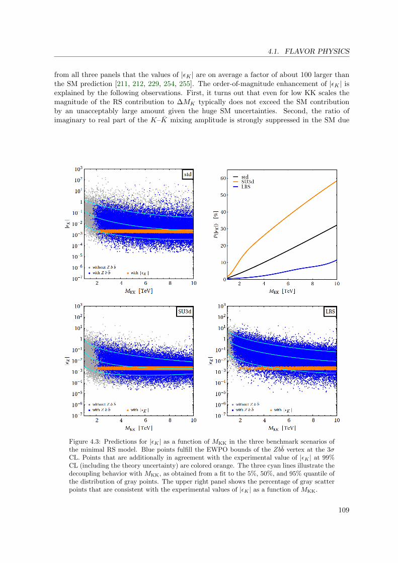
4.1. FLAVOR PHYSICS
from all three panels that the values of |εK | are on average a factor of about 100 larger thanthe SM prediction [211, 212, 229, 254, 255]. The order-of-magnitude enhancement of |εK | isexplained by the following observations. First, it turns out that even for low KK scales themagnitude of the RS contribution to ∆MK typically does not exceed the SM contributionby an unacceptably large amount given the huge SM uncertainties. Second, the ratio ofimaginary to real part of the K–K mixing amplitude is strongly suppressed in the SM due
Figure 4.3: Predictions for |εK | as a function of MKK in the three benchmark scenarios ofthe minimal RS model. Blue points fulfill the EWPO bounds of the Zbb vertex at the 3σCL. Points that are additionally in agreement with the experimental value of |εK | at 99%CL (including the theory uncertainty) are colored orange. The three cyan lines illustrate thedecoupling behavior with MKK, as obtained from a fit to the 5%, 50%, and 95% quantile ofthe distribution of gray points. The upper right panel shows the percentage of gray scatterpoints that are consistent with the experimental values of |εK | as a function of MKK.
109

4. ASPECTS OF PRECISION PHYSICS
to the smallness of Im(V ∗tsVtd
). Numerically, one finds
[ImMK∗
12
ReMK∗12
]
SM
≈−2A4λ10(1− ρ) η ηttS0(xt)/(λ2 ηcc xc) ≈ −1/150 , (4.1.69)
where S0(xt) originates from the one-loop box diagrams containing a top quark, while ηttand ηcc summarize higher-order QCD corrections in the top- and charm-quark sectors [279,327]. Under the natural assumption that the phase in (MK∗
12 )RS is of O(1), it follows that|εK |RS/|εK |SM ∼ 100. Large deviations of |εK |RS from this generic value require a certain,but mild tuning of parameters, for example an adjustment of the phase of the associatedcombination of Yukawa couplings, so that ImMK∗
12 becomes comparable to the SM value. Weverified that this tuning is mild by producing the diagrams of figure 4.3 also for fine-tuningof less than one percent and find that relevant changes in the distribution appear only forvalues of |εK | far below the allowed region; in particular, there would be a hard cutoff ofvalues |εK | . 0.1 |εK |exp, which is irrelevant for the discussion at hand.
One method to protect specifically |εK | is to arrange for common bulk-mass parameterscd ≡ cdi in the sector of the right-handed down-type quarks [254], e.g. coming from a flavorsymmetry SU(3)dc (labeled “SU3d” here). In this case, certain mixing matrices differ fromthe ones present in the RS model with hierarchical values of F (cdi). The phenomenologically
most important change occurs in the case of (∆D)mn⊗(∆d)mn, which becomes quasi-diagonal.To derive an expression for the off-diagonal elements, one has to expand the flavor matricesdefined in (3.3.158) up to O(v2/M2
KK). Employing (3.3.88), we find that the relation (3.3.159)receives the correction
(δD)mn ⊗ (δd)mn =mdmmdn
M2KK
∑
i,j
[(U †d)mi
(Ud)in
(δD)ij(U †d)mj
(Ud)jn
+(W †d)mi
(Wd
)in
(δd)ij(W †d)mj
(Wd
)jn
] (4.1.70)
from the terms in (3.3.158) involving both even C(A)m (φ) and odd S
(A)m (φ) fermion profiles.
Neglecting terms suppressed by F 2(cQi) and F 2(cQi)F2(cQj ), the elements of (δD)ij take the
form
(δD)ij =2(3 + cQi − cQj )
(3 + 2cQi)(3− 2cQj )(2 + cQi − cQj )F 2(cQi)
F 2(cQj ). (4.1.71)
An analogous expression holds in the case of (δd)ij with cQi replaced by cdi . Using a Froggatt-Nielsen like analysis, as discussed in section 3.3.6, we find that to leading order in hierarchies
(∆D)mn ⊗ (∆d)mn ∼
F (cQm)F (cQn)F (cdm)F (cdn) , “standard” ,
F (cQm)F (cQn)F 2(cd)
(δmn +
Y 2d v
2
2M2KK
), “aligned” .
(4.1.72)
We have only shown the leading order flavor-off-diagonal contribution. Notice that theO(v2/M2
KK) correction arising in the aligned case is solely due to the first line in (4.1.70)involving left-handed rotations Ud. The contribution from the second line in (4.1.70) is fur-ther suppressed, since the universality of (δd)ij ∼ 1 in combination with the unitarity of theWd matrices renders it negligibly small.
110
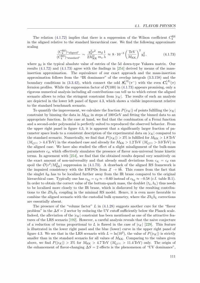
4.1. FLAVOR PHYSICS
The relation (4.1.72) implies that there is a suppression of the Wilson coefficient CRS4
in the aligned relative to the standard hierarchical case. We find the following approximatescaling
(CRS4 )“aligned”
(CRS4 )“standard”
∼ y2dv
2
2M2KK
md
ms
1
λ≈ 8 · 10−3
(TeV
MKK
)2
y2d , (4.1.73)
where yd is the typical absolute value of entries of the 5d down-type Yukawa matrix. Ourresults (4.1.72) and (4.1.73) agree with the findings in [254] derived by means of the mass-insertion approximation. The equivalence of our exact approach and the mass-insertionapproximation follows from the “IR dominance” of the overlap integrals (3.3.158) and the
boundary conditions in (3.3.42), which connect the odd S(A)n (π−) with the even C
(A)n (π)
fermion profiles. While the suppression factor of O(100) in (4.1.73) appears promising, only arigorous numerical analysis including all contributions can tell us to which extent the alignedscenario allows to relax the stringent constraint from |εK |. The results of such an analysisare depicted in the lower left panel of figure 4.3, which shows a visible improvement relativeto the standard benchmark scenario.
To quantify the improvement, we calculate the fraction P (|εK |) of points fulfilling the |εK |constraint by binning the data in MKK in steps of 100 GeV and fitting the binned data to anappropriate function. In the case at hand, we find that the combination of a Fermi functionand a second-order polynomial is perfectly suited to reproduced the observed behavior. Fromthe upper right panel in figure 4.3, it is apparent that a significantly larger fraction of pa-rameter space leads to a consistent description of the experimental data on |εK | compared tothe standard scenario. Numerically, we find that P (|εK |) > 3% is fulfilled for MKK > 1.8 TeV(MG(1) > 4.4 TeV) in the standard case and already for MKK > 1.2 TeV (MG(1) > 3.0 TeV) inthe aligned case. We have also studied the effect of a slight misalignment of the bulk-massparameters cd, which effectively simulates the presence of flavor non-universal brane kineticterms. In agreement with [254], we find that the obtained results depend very sensitively onthe exact amount of non-universality and that already small deviations from cdi = cd canspoil the O(v2/M2
KK) suppression in (4.1.73). A drawback of the aligned RS framework isthe impaired consistency with the EWPOs from Z → bb. This comes from the fact thatthe singlet bR has to be localized further away from the IR brane compared to the originalhierarchical case. Typically one has cbR = cd ≈ −0.60 instead of cbR ≈ −0.58 (c.f. table B.1).In order to obtain the correct value of the bottom-quark mass, the doublet (tL, bL) thus needsto be localized more closely to the IR brane, which is disfavored by the resulting contribu-tions to the ZbLbL coupling in the minimal RS model. Hence, it is even more favorable tocombine the aligned scenario with the custodial bulk symmetry, where the ZbLbL correctionsare essentially absent.
The presence of the “volume factor” L in (4.1.28) suggests another cure for the “flavorproblem” in the ∆S = 2 sector by reducing the UV cutoff sufficiently below the Planck scale.Indeed, the alleviation of the |εK | constraint has been mentioned as one of the attractive fea-tures of the LRS scenario [192]. However, a careful analysis reveals that the naive conjectureof a reduction of terms proportional to L is flawed in the case of |εK | [229]. This featureis illustrated in the lower right panel and the blue (lower) curve in the upper right panel offigure 4.3. We see that in the LRS scenario with L = ln(103), the value of P (|εK |) is strictlysmaller than in the standard scenario for all values of MKK. Comparing to the values givenabove, we find P (|εK |) > 3% for MKK > 4.7 TeV (MG(1) > 11.4 TeV) only. The origin ofthe enhancement of flavor-changing ∆S = 2 effects is the phenomenon of “UV dominance”,
111

4. ASPECTS OF PRECISION PHYSICS
which arises whenever the bulk-mass parameters determining the strange-quark mass satisfythe critical condition cQ2 + cd2 < −2 [229]. The relevant overlap integrals (3.3.158) are thendominated by the region near the UV brane, thereby partially evading the RS-GIM mech-anism. new physics contributions to |εK | are then exponentially enhanced with respect tothe standard scenario with L = ln(1016). While in the LRS scenarios thus no improvementconcerning |εK | is achieved unless the UV cutoff is raised above several 103 TeV, this classof models still helps to relax the constraint from Z → bb. We discuss this in more detail insection 4.2.2. Further details on variants of the RS model with volume-truncated backgroundcan be found in [229].
It should have become clear from the above discussion and explanations that the “flavorproblem” in the ∆S = 2 sector in the framework of warped extra dimensions [211, 212,229, 254, 255] depends highly on the required amount of allowed parameter space, even fornatural parameters. We showed that the huge spread caused by the RS parameter spacecombined with the slow decoupling creates difficulties on what is to be considered as a boundon the scale of the RS model. For this reason, we warn the reader that simple statementson strong bounds from |εK | found in the literature can be misleading. Instead, we quantifiedthe decoupling behavior, which allows for a detailed comparison of the standard minimal RSmodel to modified versions of the model with an SU(3)dc flavor-symmetry or with volume-truncated background. Being very conservative, we find in the standard scenario of theminimal RS model
MKK & 0.7 TeV , MG(1) & 1.7 TeV , (4.1.74)
from the total closure of the viable parameter space, i.e. P (|εK |) = 0, in our parameter setwith less than one per mil fine-tuning. This bound is similar to the one inferred from directsearches for resonances in the tt channel, which we discussed in section 4.1.2.1. A very naturalsolution with only one percent fine-tuning and P (|εK |) = 1% is obtained for
MKK & 1.5 TeV , MG(1) & 3.6 TeV . (4.1.75)
Deriving bounds from stricter requirements on the tuning are unsubstantiated in the light ofthe unsolved little hierarchy problem of the Higgs-mass value.
Rare Kaon Decays
We continue our numerical investigations with the rare decays K → πνν, KL → π0l+l−, andKL → µ+µ−. In the former case, the special role of the K → πνν and KL → π0l+l− modesis emphasized, which is due to their theoretical cleanliness and their enhanced sensitivityto non-standard flavor and CP violation. They are unique tools to potentially set severeconstraints on the RS parameter space, or find clean deviations, once they are measured.
In the lower left panel of figure 4.4, we display the predictions for the branching ratio ofthe neutral mode versus that of the charged one for the standard scenario of the minimalRS model. The blue points correspond to parameter values that satisfy the constraints fromZ → bb and |εK | as discussed in the last section. For comparison, the central value and the68% CL range Br(K+ → π+νν(γ))exp =
(1.73+1.15
−1.05
)·10−10 based on seven events in the E949
experiment [328] is indicated by the vertical dashed black line and the yellow band. Theexperimental 90% CL upper limit Br(KL → π0νν)exp < 2.6 · 10−8 [329] is not displayed inthe figure. The central values of the SM predictions (4.1.50) are indicated by the green cross.The branching fractions of both K → πνν channels can be significantly enhanced compared
112

4.1. FLAVOR PHYSICS
Figure 4.4: upper left panel: Predictions for Br(KL → π0νν) as a function of MKK. Thesolid green line represents the SM prediction. Grey points fulfill the constraint from Z → bbat the 3σ CL. Blue points additionally reproduce the value of |εK | at 99% CL. The two cyanlines are obtained from a fit to the 5% and 95% quantile of the distribution of gray points.upper right panel: Predictions for Br(K+ → π+νν(γ)) versus εK . Color coding and con-straints are the same as in the upper left panel. Additionally the median curve is displayed.lower panels: Results for Br(K+ → π+νν(γ)) versus Br(KL → π0νν) in the standardbenchmark scenario (left) and the aligned scenario (right). Color coding and constraints arethe same as in the upper panels. The gray shaded area shows the GN bound. The verticaldashed black line and the yellow band display the experimental central value and 68% CLrange. Points marked red are compatible with ε′K/εK as discussed below.
113

4. ASPECTS OF PRECISION PHYSICS
to the SM prediction. For a very small fraction of parameter space, it is even possible tosaturate the model-independent Grossman-Nir (GN) bound [330]
Br(KL → π0νν) ≤ κLκ+(1 + ∆EM)
Br(K+ → π+νν(γ)) ≈ 4.3 Br(K+ → π+νν(γ)) , (4.1.76)
The inequality (4.1.76) is indicated by the straight dotted black line in the figure, and theinaccessible area is colored gray. Because the weak phase entering the s → dνν transitioncan take essentially any value in the standard scenario, the predictions for the charged andneutral mode are mostly uncorrelated.
From the plots in the upper two panels of figure 4.4, we observe that very large deviations ofmore than a factor of two are yet disfavored by the bound on |εK |, due to a weak correlationof |εK | to both decay modes. This is displayed by the gray points, which only fulfill theZ → bb constraint and populate a much larger region for both decay modes. We illustrate thedecoupling behavior of the neutral decay mode by fits to the 5% and 95% quantile, obtainedafter a fine grained binning in MKK. In principle, the result indicates a strong sensitivity ofthe neutral mode to RS corrections even at high KK scales. However, as we will show below,the possible deviations are very restricted by the constraint following from ε′K/εK . Largeshifts in the CP -violating neutral decay mode typically appear together with an unacceptableamount of direct CP violation in K → ππ. The correlation is more pronounced than theone with εK , as shown by the red points in the lower panels of figure 4.4. We discuss thisin more detail below. Concerning the charged mode, the correlation with |εK | imposes infact the most relevant constraint on possible deviations. We illustrate in the upper rightpanel of figure 4.4 how this constraint excludes a large fraction of the parameter space, whereotherwise order-of-magnitude deviations would be possible. As can be seen from the cyanlines, which are spline interpolations of the 5%, 50%, and 95% quantiles after binning in |εK |,very large values of |εK | would allow for a large fraction of parameter space that has largedeviations in the charged decay mode. On the other hand, one should keep in mind that thecorrelation disfavors, but does not exclude certainly, large deviations in the charged mode.
While the pattern of deviations found in the LRS scenario follows that observed in thestandard case, a considerably different picture emerges in the aligned scenario, with commonbulk-mass parameters cdi = cd. This is illustrated in the lower right panel of figure 4.4. Tounderstand the observed pattern, we recall that in the aligned scenario right-handed currentsentering |εK | in form of the Wilson coefficients CRS
1 , CRS4 , and CRS
5 (see (4.1.72)) as wellas K → πνν in form of CRS
ν are parametrically suppressed by factors of v2/M2KK and thus
numerically subleading compared to the left-handed corrections CRS1 and CRS
ν . The latter areto leading order in L proportional to (∆D)12 ⊗ (∆D)12 and (∆D)12. Furthermore, the factthat the left-handed contribution (∆D)12⊗(∆D)12 factorizes as (∆D)12⊗(∆D)12 ≈ (∆D)2
12 =∣∣(∆D)12
∣∣2e2 i ϕ12 implies that |εK | as well as K → πνν are governed by the same weak phaseϕ12. The requirement |εK |RS ∝ Im
((∆D)12 ⊗ (∆D)12
)≈ 0 then forces ϕ12 in the standard
CKM phase convention (2.2.14) to be a multiple of π/2. One can show model-independentlythat in such a situation only two branches of solutions in the Br(K+ → π+νν(γ)) – Br(KL →π0νν) plane are allowed [331]. The first branch features Br(KL → π0νν) ≈ Br(KL →π0νν)SM, while the second runs through the SM point (4.1.50) with a slope approximatelyequal to the slope of the GN bound (4.1.76). The second branch of solutions is absent in thecase at hand, as we show now. To leading order in CKM hierarchies, the (1, 2) elements ofthe charged-current matrix VL and the mixing matrix ∆D take the following form in the case
114

4.1. FLAVOR PHYSICS
of alignment
(VL)12 =
[(MdM
†d)21
(MdM†d)11
− (Mu)21
(Mu)11
]F (cQ1)
F (cQ2),
(∆D)12 = −1
2
[(MdM
†d)21
(MdM†d)11
+(YdY
†d )∗23
(YdY†d )33
(MdM†d)31
(MdM†d)11
]F (cQ1)F (cQ2) ,
(4.1.77)
where Md denotes the matrix of minors of Yd. This result is derived from a Froggatt-Nielsenanalysis for the SU(3)dc symmetric case.
Sizable corrections inK → πνν necessarily correspond to large values of |(∆D)12|. |(∆D)12|grows with decreasing (YdY
†d )33 and decreasing (MdM
†d)11. Furthermore, in the anarchic
setup (YdY†d )33 has a natural size close to the square of the maximally allowed Yukawa en-
try, i.e. O(y2max). Barring accidental cancellations, we need to consider the conditions for
a vanishing product of minors. In the limit (MdM†d)11 → 0, the expressions (4.1.77) are
approximated by
(VL)12 ≈(MdM
†d)21
(MdM†d)11
F (cQ1)
F (cQ2),
(∆D)12 ≈ −1
2
[1 +
(YdY†d )22
(YdY†d )33
](MdM
†d)21
(MdM†d)11
F (cQ1)F (cQ2) ,
so that in the standard CKM phase convention (2.2.14), i.e. after rotating away the phase of(VL)12, one ends up with
(∆D)12 e−i arg(VL)12 ≈ −1
2
[1 +
(YdY†d )22
(YdY†d )33
]∣∣(MdM†d)21
∣∣(MdM
†d)11
F (cQ1)F (cQ2) < 0 . (4.1.78)
Using (4.1.37) and (4.1.47), we find that this inequality implies that Re (XRS) < 0 andIm (XRS) ≈ 0 for the quantity XRS defined in (4.1.49). Recalling that in the SM one hasRe (XSM) ≈ −1.2 and Im (XSM) ≈ 0.3, we then deduce from (4.1.48) that in the limit (4.1.78)the aligned scenario predicts constructive interference in the branching ratio of K+ → π+νν,while the KL → π0νν rate is expected to take approximately its SM value. Invoking the|εK | constraint further drives the solutions toward (4.1.78), as it singles out solutions withϕ12 ≈ π, so that Re (XRS) < 0 and Im (XRS) ≈ 0 turn out to hold in the aligned case evenwhen |(∆D)12| is small. We conclude that in the aligned scenario, the allowed points in theBr(K+ → π+νν(γ)) – Br(KL → π0νν) all lie close to a horizontal line to the right of the SMpoint (4.1.50), what is clearly observed in the lower right panel of figure 4.4.
The discussion above highlights that the K → πνν decays offer a unique tool to study thefermion geography in the down-type quark sector of models with warped extra dimensions,since they provide, in combination with |εK |, a powerful way to test the universality of new-physics contributions in ∆S = 1 and ∆S = 2 transitions. Precision measurements of theKL → π0νν and K+ → π+νν branching fractions feasible at high-intensity proton-beamfacilities such as NA62, J-PARC, and Project X should therefore be primary goals of thefuture flavor-physics program.
While theoretically not as clean as K → πνν, the KL → π0l+l− channels offer theopportunity to constraint additional ∆S = 1 effective operators that are inaccessible to
115

4. ASPECTS OF PRECISION PHYSICS
Figure 4.5: Prediction for Br(KL → π0l+l−), l = e, µ (upper left), Br(KL → π0νν) –Br(KL → π0l+l−) (upper right), and Br(KL → π0νν)–AFB(KL → π0µ+µ−) (lower panel).The green crosses indicate the SM point, while the blue scatter points fulfill the constraintfor Z → bb and |εK | as discussed in the text.
the neutrino modes. In figure 4.5, we show predictions for KL → π0l+l− with l = e, µand their correlation with the KL → π0νν mode. All plots correspond to our standardscenario including the constraint from Z → bb and |εK |. The predictions in the remainingbenchmark scenarios are essentially indistinguishable from the ones displayed. In the case ofthe KL → π0l+l− observables we have assumed constructive interference between the directand indirect CP -violating amplitudes as favored by the analyses [317, 318]. We observe thatenhancements of the branching ratio of both KL → π0l+l− modes by a factor of about 5are possible without violating any constraints. On the other hand, the RS predictions forAFB(KL → π0µ+µ−) can be smaller than the SM value by almost a factor of 10. Noticethat modifications in Br(KL → π0µ+µ−) and AFB(KL → π0l+l−) are anti-correlated, since
116

4.1. FLAVOR PHYSICS
the branching ratio enters (4.1.60) in the denominator. The pattern of the correlations seenin the upper left panel of figure 4.5 arises because the coefficient YV of the semileptonicvector operator is suppressed with respect to the coefficient YA of the axial-vector operatorby a factor of about (1 − 4s2
w) ≈ 0.08, and scalar interactions play essentially no role. Thesuppression factor stems from the coupling of the Z boson and its KK excitations to thecharged lepton pair. The ratio YV /YA determines the angle between the two possible branchesin the Br(KL → π0µ+µ−) – Br(KL → π0e+e−) plane. Since YV /YA is generically small in theRS model, the two branches are very close to each other. The correlations observed in theupper right and lower panel of figure 4.5 have a similar origin. In this case, they are a resultof the interplay of the coupling of the Z boson and its KK excitations to a pair of chargedand neutral leptons. While the former is mostly axial-vector like, the latter is purely left-handed. The observed correlations between KL → π0νν and KL → π0l+l− should thereforebe considered a generic feature of models where the couplings of heavy neutral gauge bosonsto leptons are SM-like, rather than a specific characteristic of the RS framework.
Interesting complementary information can be obtained from the KL → µ+µ− decaymode, which has been measured precisely. The predictions for Br(KL → µ+µ−) as a functionof Br(K+ → π+νν(γ)) in the parameter standard hierarchical and the aligned scenario aredisplayed in figure 4.6 including the constraint from Z → bb and |εK |. We have assumed that
Figure 4.6: Prediction for Br(K+ → π+νν(γ)) versus Br(KL → µ+µ−) in the standard andaligned scenario. The green crosses indicate the SM point, while the blue scatter pointsfulfill the constraint for Z → bb and |εK | as discussed in the text. The experimental centralvalue and 68% CL range for Br(K+ → π+νν(γ)) (vertical dashed line and yellow verticalband) as well as the 68% and 95% CL regions for Br(KL → µ+µ−) (yellow and orangehorizontal band) including both experimental and theoretical errors are shown.
the two-photon amplitude in KL → µ+µ− has positive sign, which is supported by theoreticalarguments [313]. In the case of the KL → µ+µ− branching ratio the error band includes thetheory error, which by far dominates the total uncertainty. We observe that the branchingratio of KL → µ+µ− can reach experimentally disfavored values with an enhancement ofabout 20% relative to both the SM prediction and the measured value. A mostly positivelinear correlation between K+ → π+νν and KL → µ+µ− is visible. This correlation originates
117

4. ASPECTS OF PRECISION PHYSICS
from the fact that K+ → π+νν measures the vector, while KL → µ+µ− measures the axial-vector component of the Zds vertex. Since the SM flavor-changing Z penguin is purelyleft-handed and the RS contribution is dominated in our case by the very same component,the SM and new-physics contributions enter both decay modes with the same sign. Noticethat the correlation is more pronounced in the aligned scenario, because the right-handedcontributions to the Zds vertex are further suppressed in this benchmark scenario. In a RSvariant with custodial protection, the correlation between K+ → π+νν and KL → µ+µ− hasexpected to be inverse to the minimal model shown here, since the given quark embedding(3.3.66) implies a simultaneous protection of all Zdidj couplings. This has been confirmed in[261]. Hence, precision measurements of K+ → π+νν accompanied by theoretical progressin the prediction of KL → µ+µ− would allow one to identify the chiral structure of the Zdsvertex and in this way could select between different models of non-standard interactions.
We close this section with a comparison to the expected results in the RS model withcustodial protection. Employing the quark embedding (3.3.66), we found in (3.3.142) thatthe ratios of the corrections to the flavor-changing Z-boson couplings in the minimal andcustodial model are given by
(δgdL)custoij
(δgdL)minimalij
= − (1/2− s2w/3) (∆′D)ij
(1/2− s2w/3) (L (∆D)ij − (∆′D)ij)
≈ − 1
L,
(δgdR)custoij
(δgdR)minimalij
= −c2w L (∆d)ij − s2
w/3 (∆′d)ijs2w/3 (L (∆d)ij − (∆′d)ij)
≈ −3c2w
s2w
, (4.1.79)
where we use (∆D,d)ij ≈ (∆′D,d)ij . A suppression factor for the left-handed couplings ofroughly 100 has been claimed in [212, 261] using the diagonalization of large mass matrices.We observe that the origin of this suppression is very clear in our analytic approach. On theother hand, we find that the Z0di Rdj R vertices in the model with custodial protection areenhanced in magnitude by a factor of about 10 relative to the original RS formulation, whichis in accordance with [212, 261]. From (4.1.79), we also observe that
(gdR)custoij
(gdL)minimalij
≈ − c2w
1/2− s2w/3
(∆d)ij(∆D)ij
≈ −2(∆d)ij(∆D)ij
≈ −2F (cdi)F (cdj )
F (cQi)F (cQj ). (4.1.80)
To arrive at this relation, we used that the bulk masses do not depend on whether oneconsiders the custodially protected or the original RS model, since the cAi parameters aredetermined by the quark masses and mixings. In order to have effects in rare kaon decaysof similar magnitude in the custodially protected and the original RS model requires theproducts F (cd1)F (cd2) and F (cQ1)F (cQ2) to be of similar size. Yet the locations of the zero-modes are not unique solutions [200], a feature that manifests itself in the invariance undera set of reparametrization transformations [1]. In particular, a simultaneous rescaling of thefermion profiles for SU(2)L doublet and singlet fields by opposite factors, while leaving the5D Yukawa couplings invariant, allows one to redistributes effects between the left- and right-handed sectors. This freedom can be used to express (F (cd1)F (cd2))/(F (cQ1)F (cQ2)) throughthe quark masses, Wolfenstein parameters, and F (cu3). To leading power in hierarchies wefind the scaling relations
∣∣∣∣(gdR)custo
12
(gdL)minimal12
∣∣∣∣ ∼mdms y
4uv
2
2A4 λ10m4t y
2d
F (cu3)4 ≈ 0.08y4u
y2d
F (cu3)4 , (4.1.81)
118

4.1. FLAVOR PHYSICS
which implies that the ratio of right- to left-handed Zds couplings can be enhanced by lo-calizing the right-handed top quark closer to the IR brane. We observe that the degree ofcompositeness of the top quark thus plays a crucial role in this context. For comparison wegive the numerical values 0.08F (1)4 = 0.7 and 0.08F (2)4 = 2.0. Analogous formulas hold inthe case of the Z → bd and bs transitions with (mdms)/(A
4λ10) replaced by (mdmb)/(A2λ6)(
(msmb)/(A2λ4)
). The corresponding numerical factors (4.1.81) are 0.006 and 0.005 instead
of 0.08. Hence, barring accidental cancellations and given bulk that do not exceed the curva-ture scale by far, we expect a relative suppression in the custodial setup as compared to theminimal setup of at least an order of magnitude for rare B decays.
Analysis of Bq → µ+µ−
The predictions for Br(Bs → µ+µ−) versus Br(Bd → µ+µ−) as obtained from a parameterscan in the standard scenario are displayed in figure 4.7. The two other benchmark scenariosshow a similar distribution. We observe that even after imposing of the Z → bb constraints
Figure 4.7: Prediction for Br(Bq → µ+µ−), q = d, s in the standard scenario of the minimalRS model. The green crosses indicates the SM point. The blue scatter points fulfill theZ → bb constraints as discussed in the text. The experimental and 95% CL exclusion regionfor the Bd and the 68% and 95% CL for the Bs mode from LHCb are marked with red,yellow, and orange, respectively. The gray dashed line represents the correlation found inCMFV models.
large uncorrelated enhancements by a factor of 3–4 are possible in both the Bd and Bs decaymodes without violating existing constraints. The uncorrelated distribution implies that largedeviations from the relation [332]
Br(Bs → µ+µ−)
Br(Bd → µ+µ−)=f2BsmBsτBs |Vts|2
f2BdmBdτBd |Vtd|2
≈ 32.8 , (4.1.82)
which is valid in models with constrained MFV (CMFV) [333], are possible in the RS model.The measurement of the Bs mode by LHCb [260] already constrains a small part of the RSparameter space in the minimal model. We have mentioned in section 4.1.2.2 that the error of
119

4. ASPECTS OF PRECISION PHYSICS
the measurement has small systematic errors and still exceeds the uncertainty of the theoryprediction by a factor of 5, such that this mode will unfold a strong constraining power inthe near future, given the central value remains compatible with the SM. The existing limitin the case of Bd → µ+µ− is much weaker and not expected to become very relevant soon,and has to await further investigations at a super flavor factory.
We refer to the previous paragraph for a comparison of the expected changes in going tothe custodial setup presented in section 3.3.5.2, where we found a suppression of at least oneorder of magnitude for the RS contributions. A similar result was found in [261].
Analysis of ε′K/εK and its Effect on Rare Kaon Decays
Within the SM the smallness of direct CP violation in K → ππ is the result of a destruc-tive interference between the positive contribution due to QCD penguins and the negativecontribution arising from electroweak penguin diagrams. In new-physics models in which the∆I = 1/2 and ∆I = 3/2 contributions to s → dqq processes are affected differently fromeach other, this partial cancellation is usually much less pronounced or even absent. A qual-itative understanding of the situation in the minimal RS model can be obtained from theapproximate relation
(ε′KεK
)
RS
∝ 1 + [−0.1, 0.1]B(1/2)6 − 12B
(3/2)8 , (4.1.83)
which has been obtained from the second expression in (4.1.40) by inserting typical valuesof the Wilson coefficients CRS
3−10 and CRS3−10. The smallness of the coefficient multiplying the
hadronic parameter B(1/2)6 compared to the coefficient of B
(3/2)8 is easily explained by the
structure of ε′K/εK within the SM. While both the QCD and electroweak penguin contribu-tions are strongly enhanced by RG effects, the QCD correction results mainly from the mixingof Q6 with Q1,2. Thus, it is essentially unaffected by new physics. On the other hand, mixingwith the current-current operators plays only a minor role in the case of the electroweakpenguins, so that any new-physics contribution to the initial conditions in this sector directlyfeeds through into ε′K/εK . This implies that electroweak penguin operators give the dominantRS correction to direct CP violation in the kaon sector. Our numerical analysis confirms thismodel-independent conclusion. Notice that the sign of (ε′K/εK)RS in (4.1.83) is not fixed, sothe prediction for the total ratio ε′K/εK can be both positive or negative. An enhancementoccurs in the case of an electroweak penguin contribution that has opposite sign with respectto the SM Z-penguin amplitude, and vice versa.
The observables ε′K/εK and |εK | are not independent from each other, if ε′K/εK is calcu-lated fully in theory. Since the central value of the theory prediction for ε′K/εK (4.1.45) isbelow the experimental world average, models with new positive contributions to |εK | andnegative contributions to ε′K are disfavored. The correlation between ε′K/εK and |εK | in thestandard scenario is shown in the left panel of figure 4.8. Like before, points that are consis-tent with the constraints from Z → bb at the 3σ CL are colored blue. Points marked orangeare furthermore compatible with |εK | at the 99% CL after combining theory and experimen-tal uncertainty, and they can be brought into agreement with the experimental 95% CL ofε′K/εK when scanning over the conservative ranges in (4.1.44) for the non-perturbative inputparameters R6,8 and light masses. The abscissa value of each point is obtained by setting thenon-perturbative parameters R6,8 equal to 1 and light quark masses to their central values.It is evident from the distribution of points that solutions featuring excluded values of |εK |
120
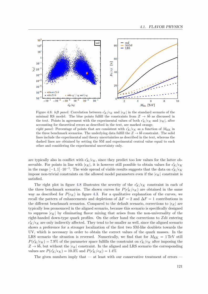
4.1. FLAVOR PHYSICS
Figure 4.8: left panel: Correlation between ε′K/εK and |εK | in the standard scenario of theminimal RS model. The blue points fulfill the constraints from Z → bb as discussed inthe text. Points in agreement with the experimental values of both ε′K/εK and |εK |, afteraccounting for theoretical errors as described in the text, are marked orange.right panel: Percentage of points that are consistent with ε′K/εK as a function of MKK inthe three benchmark scenarios. The underlying data fulfill the Z → bb constraint. The solidlines include the experimental and theory uncertainties as described in the text, whereas thedashed lines are obtained by setting the SM and experimental central value equal to eachother and considering the experimental uncertainty only.
are typically also in conflict with ε′K/εK , since they predict too low values for the latter ob-servable. For points in line with |εK |, it is however still possible to obtain values for ε′K/εKin the range [−1, 1] · 10−1. The wide spread of viable results suggests that the data on ε′K/εKimpose non-trivial constraints on the allowed model parameters even if the |εK | constraint issatisfied.
The right plot in figure 4.8 illustrates the severity of the ε′K/εK constraint in each ofthe three benchmark scenarios. The shown curves for P (ε′K/εK) are obtained in the sameway as described for P (εK) in figure 4.3. For a qualitative explanation of the curves, werecall the pattern of enhancements and depletions of ∆F = 2 and ∆F = 1 contributions inthe different benchmark scenarios. Compared to the default scenario, corrections to |εK | aretypically less pronounced in the aligned scenario, because this scenario is specifically designedto suppress |εK | by eliminating flavor mixing that arises from the non-universality of theright-handed down-type quark profiles. On the other hand the corrections to Zds enteringε′K/εK are only indirectly affected. They tend to be smaller as well, since the aligned scenarioshows a preference for a stronger localization of the first two SM-like doublets towards theUV, which is necessary in order to obtain the correct values of the quark masses. In theLRS scenario the situation is reversed. Numerically, we find that for MKK = 1 TeV stillP (ε′K/εK) = 7.9% of the parameter space fulfills the constraint on ε′K/εK after imposing theZ → bb, but without the |εK | constraint. In the aligned and LRS scenario the correspondingvalues are P (ε′K/εK) = 10.3% and P (ε′K/εK) = 1.4%
The given numbers imply that — at least with our conservative treatment of errors —
121

4. ASPECTS OF PRECISION PHYSICS
we are not able to derive a precision constraint from ε′K/εK . This is in contrast to thesituation for |εK |, due to the very precise measurement of the latter parameter and a muchbetter control over theory uncertainties. We also show by the dashed lines in the plot forP (|εK |) in figure 4.8 that even a major improvement in the theoretical understanding of thenon-perturbative input will not render ε′K/εK a precision test of the RS scale MKK. Theselines are obtained for the hypothetical scenario that the SM and experimental central valuesare equal and assuming a 20% theory uncertainty, which we combine quadratically with theexperimental error. Instead, the bound from ε′K/εK is very interesting and relevant because ofits impact on the Yukawa structure and the restrictions it imposes on other flavor observables,namely CP -violating rare K decays, as we will see below.
Before that, we must mention that potentially large corrections to ε′K/εK could arise fromthe presence of the chromomagnetic dipole operator Qg8 and its chirality-flipped partner Qg8.In the context of scenarios with hierarchical fermion profiles, this issue has been analyzedin a model-independent way in [334]. Interestingly, the contributions to ε′K/εK from Cg8and Cg8 and to εK from CRS
4 depend in an opposite way on the absolute size of the Yukawacouplings. This makes it difficult to decouple flavor-violating effects in εK by using largeYukawa couplings, and it will lead to a tension between tree- and loop-level effects, similarto what happens in the case of B → Xsγ and εK [255]. A study of this anti-correlationincluding the first KK level of the quarks and the zero-mode of a bulk Higgs field has beenpresented recently in [335]. There, it has been pointed out that the NDA estimate for thetypical size of the the chromomagnetic dipole-operator contribution leads to a value of ε′K/εKthat, when combined with the NDA estimate for |εK |, becomes compatible with the measuredvalue only for MG(1) > 5.5 TeV, if the Higgs boson is maximally spread into the bulk. Thisvalue is raised to 7.5 TeV if one considers the case of the two-site model [255]. It is importantto realize that the quoted numbers are no “bounds” in the strict terminology we use here.They neglect the full parameter distribution, which is found to be widely spread. Moreover,the numbers are obtained for typical values of the down-type quark Yukawa couplings (yd =4.6 and yd = 5.9) that are larger than the value ymax = 3 allowed by perturbativity inour benchmark scenarios. We estimate the chromomagnetic dipole contribution to ε′K/εK ,utilizing the formulas presented in [335]. We find that the chromomagnetic contribution toε′K/εK is smaller than the electroweak penguin contribution for perturbative Yukawa matrices;to this end, we express the additional contribution to ε′K/εK arising from Qg8 and Qg8 as F gRS,which has to be added to FRS in (4.1.40). Using the central values for cQ1,2 quoted in table B.1,we compare F gRS to the largest contribution of in FRS, which arises from the Wilson coefficientCRS
7 . Applying furthermore a Froggatt-Nielsen analysis to leading order in the Cabibbo angle,we find approximate typical values of
|F gRS| ≈ 2.5 · 10−3B(1/2)g fg
(1 TeV
MKK
)2
, |FRS| ≈ 1.0 · 10−2B(3/2)8 f8
(1 TeV
MKK
)2
, (4.1.84)
where B(1/2)g ≈ 1 denotes the hadronic parameter related to the matrix element of Qg8, while
fg, and f8 are functions of ratios of Yukawa couplings and thus naturally of O(1). It followsthat after requiring the correct quark hierarchies, the corrections due to the chromomagneticdipole operators are typically an order of magnitude smaller than those arising from theelectroweak penguin sector. This justifies to ignore effective couplings in ε′K/εK generatedfirst at the one-loop level in the discussion at hand.
The marked sensitivity of ε′K/εK to modifications of the electroweak penguin sector leadsto stringent correlations between ε′K/εK and the s → dνν, s → dl+l− observables. This
122

4.1. FLAVOR PHYSICS
feature is illustrated in Figure 4.9, where the left panel shows the predictions for ε′K/εK asa function of the branching fraction of KL → π0νν in the standard scenario. There, we
Figure 4.9: Correlation between Br(KL → π0νν) and ε′K/εK in the standard scenario of theminimal RS model. All points fulfill constraints from Z → bb and |εK | as described in thetext. The blue points correspond to the central value for ε′K/εK obtained for R6,8 = 1. Thered/green points illustrate the maximal/minimal achievable values of ε′K/εK for the sameset of points, as obtained by varying the hadronic parameters in the ranges (4.1.44). Forcomparison, the experimental 95% CL on ε′K/εK is displayed.
show three vertically displaced distributions. They are based on the same set of parameterpoints as used above imposing both the constraint from Z → bb and εK . For each point weplot three values of ε′K/εK , one in blue corresponding to fixed central values of the hadronicparameters R6,8 = 1 and light quark masses, one in red obtained by maximizing ε′K/εK fromusing the range of hadronic parameters and light quark masses given in (4.1.44), and one ingreen for the minimal possible value. This is analogous to the scan used in in figure 4.8. Thelight gray band represents the experimental 95% CL. We observe that an enhancement of theCP -violating Br(KL → π0νν) tends to be accompanied by a suppression of ε′K/εK , and viceversa. This implies that large enhancements of the former decay mode are disfavored by the
measured amount of direct CP violation in K → ππ. Notice that values of B(3/2)8 near the
upper end of the range shown in (4.1.44) are particularly problematic in this respect, sincethey amplify the electroweak penguin contributions to ε′K/εK . Since enhancements of thebranching fractions KL → π0νν and KL → π0l+l− are strongly correlated with each other,similar statements apply to the rare kaon decay modes with charged leptons in the finalstate. The same strong anti-correlation between Br(KL → π0νν) and ε′K/εK is also presentin the LRS parameter scenario and it even effectively constrains the correlated distributionbetween Br(KL → π0νν) and Br(K+ → π+νν) found in the aligned model. It arises sinceboth observables receive the dominant correction from the imaginary part of the left-handedZds amplitude, which enters linearly and with opposite sign relative to the SM contributionin ε′K/εK , whereas it appears quadratically and with the same sign in Br(KL → π0νν). Weconclude that even with a conservative treatment of errors, ε′K/εK has a very relevant impacton the possible new-physics effects in rare K decays within the RS model.
123

4. ASPECTS OF PRECISION PHYSICS
4.2 Electroweak Precision Measurements
In this section we introduce some of the most important electroweak precision observables(EWPOs) and discuss the strong constraint they put on deviations from the SM. We reviewup-to-date analyses that significantly impact the constraints on models of new physics. Fi-nally, we present detailed numerical consequences in the RS model. There, an analysis with afew effective parameters leads to a good understanding of the qualitatively different boundson the parameter space and the efficacy of model-building solutions that are used in order torelax the bounds.
As an outlook, we remark that the observables discussed here are an excellent field ofapplication for the sum rules presented in section 3.1.2. They can assist in identifying theconstraining properties on different sectors in perturbatively unitary theories and distinguishthem against more general contributions. Such an analysis, analogous to the one for FCNCspresented in section 4.1, is left for future work.
4.2.1 Common Observables and Effective Parameters
4.2.1.1 General Discussion and Choice of Input Parameters
The most constraining observables in the class of EWPOs are related to properties of theelectroweak gauge bosons, which were precisely measured in large data sets of e+– e− collisionsat LEP and SLC in the early 90s. Later, LEP 2 extended the knowledge of the W boson’sproperties, and the Tevatron experiments improved W and top mass measurements. Veryrecently the LHC Higgs-mass measurement added valuable information to the overall picture.
In general, an EWPO can be categorized into one of the three classes: low energy observ-ables, measurements at the Z pole, and direct mass measurements. The most important lowenergy observables stem from results on elastic neutrino–electron scattering, deep-inelasticneutrino–nucleon scattering, the τ lifetime, atomic parity violation (e.g. in Caesium), and theanomalous magnetic moment of the muon9. The latter shows a long-standing 3.0σ deviationfrom the SM theory calculation, which could be due to statistical fluctuations, underestima-tion of theory uncertainties, or indeed new physics; but the situation is inconclusive. We willnot go into further detail on the low-energy observables and refer to [337] for a comprehensivereview. Flavor-violating observables are usually not considered in this context. We consideredconstraints from off-diagonal flavor transitions separately in section 4.1.
Precision observables at the Z pole can either be constructed from the total and partialwidths ΓZ and Γff ≡ Γ(Z → ff), or from asymmetries. From the former, one obtains thetotal resonant cross section with hadronic final states σhad = 12π Γee Γhad/(M
2Z ΓZ), defines
the width ratios Rq ≡ Γqq/Γhad for identifiable primary quarks in the hadronic final state(q = c, b), and Rl ≡ Γhad/Γll for l = e, µ, τ . Here, Γhad ≡
∑q=u,d,s,c,b Γqq is the partial width
for decay into hadrons. The three measured values Γll are consistent with lepton universality.Additionally one uses the invisible-decay width Γinv ≡ ΓZ −
∑l Γll − Γhad to determine that
the number of neutrino flavors with mass much less than MZ/2 is 2.984(9) [338].
The standard formulas10 for the asymmetries at the Z pole use the definition of the
9The anomalous magnetic moment of the electron is measured even more precisely, but effects of newphysics are suppressed generically by O(me/mµ) in comparison to the muon anomalous magnetic moment. Itis instead currently used to determine the fine structure constant α [336].
10This discussion hides certain radiative corrections that we take into account below, see e.g. (4.2.14).
124

4.2. ELECTROWEAK PRECISION MEASUREMENTS
asymmetry parameter
Af =
(gLZff
)2 −(gRZff
)2(gLZff
)2+(gRZff
)2 . (4.2.1)
Using a fully polarized initial e− beam, SLD (at SLC) [339] measured the left–right asymme-tries which are asymmetries between cross sections for left- and right-handed incident elec-trons. They are directly equal to Ae. The forward–backward asymmetries for other fermionsare given by
A(Pe,f)FB =
3
4Af
Ae + Pe1 + PeAe
, (4.2.2)
and were extracted in experiments at LEP (Pe = 0) and SLC (Pe = 1).11 In the SLDexperiment this was extracted from double left–right forward–backward asymmetries
A(1,f)FB =
σfLF − σfLB − σ
fRF + σfRB
σfLF + σfLB + σfRF + σfRB=
3
4Af , (4.2.3)
for final states with f = b, c, s, τ, µ. Very precise information was added at LEP by measure-
ments of A(0,f)FB for the same final states and also for f = e. The multiplicity of asymmetry
parameters advantageously cancels systematic uncertainties to a large extent in the difference(e.g. detector asymmetries) and quotient (e.g. overall normalizations). The lepton asymme-tries are very sensitive to s2
w because of the proximity of s2w to 1/4. We illustrate this by
inserting the SM SU(2)L charges of the tree-level couplings and expanding
Af =(T 3fL − s2
wQf )2 − (s2wQf )2
(T 3fL − s2
wQf )2 + (s2wQf )2
(4.2.4)
=1− |Qf |
1− |Qf |(1− |Qf |/2)+
|Qf |2(1− |Qf |/2)
(1− |Qf |(1− |Qf |/2))2(1− 4s2
w) +O(1− 4s2w)2 .
The constant term vanishes precisely for |Qf | = 1. Ae,µ,τ thus allow us to determine theweak angle. The measurement of Af then defines the effective angle sin2(θleff), as opposedto s2
w, which was defined by the ratio of bare gauge couplings and not directly expressedby observable quantities. Alternative definitions of the weak mixing angle using input datainduce e.g. the on-shell angle s2
os = 1 −M2W /M
2Z or the weak angle given in terms of very
precise electroweak input sin2(2θ0) = (4πα(MZ)/(√
2GFM2Z))1/2. The best definition of the
weak mixing angle in the presence of new physics is often a question of convenience. Usingsl 2eff or s2
0 is favorable, since they present very precise input. Equation (4.2.4) holds true inmodels of new physics where the corrections to Z–lepton couplings are at least universal forboth chiralities, and to a large extent also lepton-flavor universal. Then the effective weakangle is an obvious choice of input. The asymmetries of the down quarks are in comparisonrather insensitive to s2
w, by a factor of almost 100, and provide a good precision constraint inmany models of new physics.
The maximal set of EWPOs considered in standard global fits of the SM parameterscontains approximately 40 observables. To constrain models of new physics, model-adaptedtechniques or effective parameters usually reduce the relevant set to a few observables. Beforewe discuss this approach in more detail we summarize the fit in the SM.
11Similar measurements were also carried out at Tevatron for e+e− final states [340], however with lessprecision due to the difficulty to disentangle qq in the underlying initial pp Drell-Yan process.
125

4. ASPECTS OF PRECISION PHYSICS
Tools for sophisticated, statistically rigorous analyses are available, like ZFITTER [341],GAPP [342], and the recently developed modular toolkit GFITTER [343]. GFITTER onlyuses the 14 most important observables but is actively developed and updated with stateof the art theoretical input. A recent evaluation from this group [344] takes into accountthe Higgs-mass value Mh = 125.7 ± 0.4 GeV reported by ATLAS and CMS in July 2012(average of [22, 29]). They find a p-value of 0.07 for the SM to describe the 14 observables,corresponding to 1.8σ. The compatibility of the fit result with the measurements is displayedin the left panel of figure 4.10 as a pull for each observable. No single observable shows adeviation of more than 3σ. However, one aspect of the updated analysis attracts interest.While overall the SM is still fully compatible with experimental data, the inclusion of a recentcalculation of two-loop electroweak corrections to Rb [345] has impaired the fit. It presents
the second largest deviation, close to the tension in A(0,b)FB . Deviations of this kind are not
unusual in a large set of observables; however it is remarkable that they are both related tothe couplings of the Z boson to b quarks. We take this as a phenomenological motivation todiscuss b-related EWPOs in more detail below.
The global SM fit also confirms the spectrum of the bosons related to electroweak symme-try breaking. Leaving the direct Higgs-mass measurement aside, [344] obtains a fit result ofMh = 94+25
−22 GeV consistent with the direct measurement. Similarly, one can also indirectlydetermine the W -boson mass. At first sight, obvious input for that purpose is the weakmixing angle in order to use the relation M2
W = e2/(4√
2s2wGF ). The weak mixing angle has
been measured over a wide range of energy scales. The most precise direct determinationis obtained from polarization asymmetries measured at Z-pole energies, as discussed above,sl 2eff = 0.23153±0.00016 [338]. Remarkably, this angle can be extracted indirectly from the fitwith a precision that supersedes the direct measurements. Moreover, the indirect determina-tion of the W -boson mass with the full set of EWPOs, MW = 80.359± 0.011 GeV, is at thesame level of precision as the SM prediction with the minimal set of input parameters that wedescribe below. The strong effect of the direct Higgs-mass measurement in over-constrainingthe SM is illustrated in the right panel of figure 4.10. We observe a shrinkage by a factor ofapproximately 3 in the CL ranges of the W -boson mass, when including the direct Higgs-massmeasurement (blue) compared to ignoring it (gray).
As already mentioned, we must choose a set of input parameters in order to predict theEWPOs in the model under consideration. Besides the Higgs mass Mh, the fermion massesmc, mb, mt, and the strong coupling constant αs, a particularly useful choice is given bythe set of Z-boson mass MZ , the fine structure constant α(M2
Z), and the Fermi constantGF . The Fermi constant is measured with a high precision from the muon decay constantGF = 1.1663787(6)× 10−5 GeV−2 [69]. We summarize the input values used in the followingin appendix B.2. The SM relation GF = 1/(
√2v2
SM) fixes the value of the SM VEV vSM.However, in models of new physics, this relation is not necessarily fulfilled. After havingworked out a theory and its symmetry breaking in terms of fundamental VEVs, one mustcarefully relate those VEVs to the muon decay and properly derive the relation to vSM. Inmost models of new physics, a SM-like Higgs doublet (or an appropriate linear combinationfrom a bidoublet in left–right symmetric models) is included and carries a VEV v, such thatit is useful to define the ratio κv ≡ v/vSM.
126
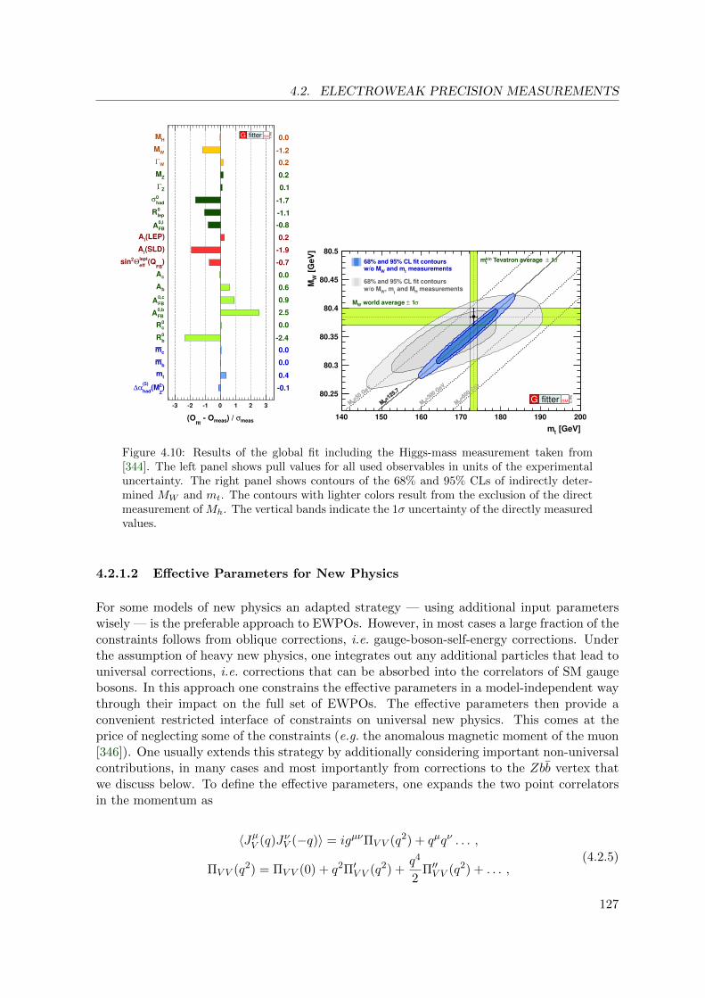
4.2. ELECTROWEAK PRECISION MEASUREMENTS
measσ) / meas Ofit
(O
3 2 1 0 1 2 3
)2
Z(M
(5)
hadα∆
tm
bm
cm
b
0R
c
0R
0,b
FBA
0,c
FBA
bA
cA
)FB
(Qlept
effΘ
2sin
(SLD)l
A
(LEP)l
A
0,l
FBA
lep
0R
0
hadσ
ZΓ
ZM
WΓ
WM
HM
0.1
0.4
0.0
0.0
2.4
0.0
2.5
0.9
0.6
0.0
0.7
1.9
0.2
0.8
1.1
1.7
0.1
0.2
0.2
1.2
0.0G fitter SM
Sep 1
2
[GeV]tm
140 150 160 170 180 190 200
[G
eV
]W
M
80.25
80.3
80.35
80.4
80.45
80.5
=50 GeV
HM=125.7
HM=300 G
eV
HM=600 G
eV
HM
σ 1± Tevatron average kint
m
σ 1± world average WM
=50 GeV
HM=125.7
HM=300 G
eV
HM=600 G
eV
HM
68% and 95% CL fit contours measurements
t and m
Ww/o M
68% and 95% CL fit contours
measurementsH
and Mt
, mW
w/o M
G fitter SM
Sep 1
2
Figure 4.10: Results of the global fit including the Higgs-mass measurement taken from[344]. The left panel shows pull values for all used observables in units of the experimentaluncertainty. The right panel shows contours of the 68% and 95% CLs of indirectly deter-mined MW and mt. The contours with lighter colors result from the exclusion of the directmeasurement of Mh. The vertical bands indicate the 1σ uncertainty of the directly measuredvalues.
4.2.1.2 Effective Parameters for New Physics
For some models of new physics an adapted strategy — using additional input parameterswisely — is the preferable approach to EWPOs. However, in most cases a large fraction of theconstraints follows from oblique corrections, i.e. gauge-boson-self-energy corrections. Underthe assumption of heavy new physics, one integrates out any additional particles that lead touniversal corrections, i.e. corrections that can be absorbed into the correlators of SM gaugebosons. In this approach one constrains the effective parameters in a model-independent waythrough their impact on the full set of EWPOs. The effective parameters then provide aconvenient restricted interface of constraints on universal new physics. This comes at theprice of neglecting some of the constraints (e.g. the anomalous magnetic moment of the muon[346]). One usually extends this strategy by additionally considering important non-universalcontributions, in many cases and most importantly from corrections to the Zbb vertex thatwe discuss below. To define the effective parameters, one expands the two point correlatorsin the momentum as
〈JµV (q)JνV (−q)〉 = igµνΠV V (q2) + qµqν . . . ,
ΠV V (q2) = ΠV V (0) + q2Π′V V (q2) +q4
2Π′′V V (q2) + . . . ,
(4.2.5)
127

4. ASPECTS OF PRECISION PHYSICS
where JµV is the current that couples to Vµ in the Lagrangian. We employ the classicalparametrization by Peskin and Takeuchi12 for the terms up to q2 in the basis of mass eigen-states [348, 349]:
S =16πs2
wc2w
e2
[Π ′ZZ(0) +
s2w − c2
w
swcwΠ ′ZA(0)−Π ′AA(0)
],
T =4π
e2c2wM
2Z
[ΠWW (0)− c2
w ΠZZ(0)− 2 swcw ΠZA(0)− s2w ΠAA(0)
],
U =16πs2
w
e2
[Π ′WW (0)− c2
w Π ′ZZ(0)− 2 swcw Π ′ZA(0)− s2w Π ′AA(0)
].
(4.2.6)
These parameters are defined relative to a fixed set of SM values, where they are usually setto zero. Gauge invariance guarantees that ΠAA(0) = 0 to all orders in perturbation theory,and one furthermore has ΠZA(0) = Π ′ZA(0) = 0 when working at tree level. The parameterT thus is sensitive to the difference between the corrections to the W - and Z-boson vacuum-polarization functions and measures isospin violation. Usually, T expresses isospin breaking
in the quotient of W and Z masses via the relation ρ0 ≡ M2W
c2wM2ZρSM
= (1 − αT )−1 ≈ 1 + αT .
This relation holds for instance for the case of an extra, heavy, non-degenerate multipletof chiral fermions or scalars. However, universal factors in the fermion couplings are alsoabsorbed into the definitions (4.2.5) and (4.2.6). In that sense, T is more general and suitableas an effective parameter. S is related to the difference of contributions to the Z-boson selfenergy at p2 = M2
Z and p2 = 0; the sum S + U is related to the analogous difference in theW -boson self energies. All three parameters are defined with a factor of α removed from theself energies such that they are expected to be of order unity in the presence of new physics.
The parameter U is only marginally affected in most models of new physics. This isexpected due to the dimensionality of the corresponding effective operator in the operatorproduct expansion in v/MNP, where MNP is the scale of new resonances. In the SU(2)L ×U(1)Y symmetric phase, S and T are proportional to the coefficients of the dimension-6
operators(Φ†T aΦ
)W aµνB
µν and∣∣Φ†Da
µΦ∣∣2, whereas U is proportional to the coefficient of the
dimension-8 operator∣∣Φ†W a
µνΦ∣∣2.
There exist four further parameters necessary to describe the modifications in (4.2.5) atfourth order in the momentum. Only two of them receive contributions from dimension-6 operators, namely (∂ρBµν)2 and (Da
ρWµν)2. In [350], the coefficients are defined in theelectroweak eigenbasis as
Y =g′M2
W
2
(s2wΠ′′ZZ(0)− 2cwswΠ′′ZA(0) + c2
wΠ′′AA(0)),
W =gM2
W
2
(c2wΠ′′ZZ(0) + 2cwswΠ′′ZA(0) + s2
wΠ′′AA(0)).
(4.2.7)
Those two parameters are useful in order to disentangle the information provided by LEP 2experiments on e+– e− cross sections at center-of-mass energies 189–207 GeV, above the Zpole [351]. However, the resulting constraints are small in most models of new physics, dueto small contributions to Y and W . In [352], it was recognized that the original S, T , and Uparameters are affected in the presence of W and Y , leading to the effective parameters
Seff = S − 4s2w
α(W + Y ) , Teff = T − s2
w
α c2w
Y , (4.2.8)
12An alternative parametrization by Altarelli and Barbieri [347] can be translated into the one given here.
128

4.2. ELECTROWEAK PRECISION MEASUREMENTS
which enter the calculations of EWPOs in the same way as S and T do when Y = W = 0.The experimental 68% CL bounds on the S, T , and U parameters and their correlation
matrix are given in [344]
S = 0.03± 0.10 ,
T = 0.05± 0.12 ,
U = 0.03± 0.10 ,
ρ =
1.00 0.89 −0.540.89 1.00 −0.83−0.54 −0.83 1.00
, (4.2.9)
and with the constraint U = 0 imposed, as
S|U=0 = 0.05± 0.09 ,
T |U=0 = 0.08± 0.07 ,ρ|U=0 =
(1.00 0.910.91 1.00
). (4.2.10)
The log likelihood for model testing, given the above values, is constructed by
χ2 =∑
i,j
(Xi,NP −Xi, obs−ref)(σ2)−1ij (Xj,NP −Xj, obs−ref) , (4.2.11)
where σ2ij = σ(Xi, obs−ref) ρij σ(Xj, obs−ref) is the covariance matrix. The Xi, obs−ref are the
values given in (4.2.9) or (4.2.10) with the subtraction of the fixed SM reference point, whichcorrespond to the input values compiled in appendix B.2. Remark that conventionally oneneglects the top mass uncertainty and considers it separately. The approximate one-loopcontribution is given by [348]
∆S = − 1
6πln
(m2t
m2t, ref
), ∆T =
3
16πs2wc
2w
m2t −m2
t, ref
m2Z
, ∆U =1
2πln
(m2t
m2t, ref
). (4.2.12)
This does also apply to the numerical values given above. The shift ∆T = ±0.013, obtainedfor the 1σ CL of the top mass, is numerically relevant.
It is interesting to evaluate the shifts of the oblique parameters due to a Higgs massdifferent from the one measured. Keeping only the leading logarithmic loop effects in the SM,they are [349]
∆S =1
12πln
(M2h
M2h, ref
), ∆T = − 3
16πc2w
ln
(M2h
M2h, ref
), ∆U = 0 . (4.2.13)
while U remains unchanged. Before the direct Higgs-mass measurement, in many modelsof new physics it turned out to be an interesting option to cancel contributions to the Sparameter with a larger Higgs mass. E.g. in [1] we speculated that high values of Mh werepossible and natural in the context of the minimal RS model. Similar options were present inthe context of the two-Higgs-doublet model and models with a fourth chiral fermion generation[353]. This underlines the strong qualitative impact that the discovery of the Higgs boson hasalready had on the search for new physics.
4.2.1.3 Precision Observables from Z → bb
We often have to consider additional non-universal EWPOs, as mentioned above. Mostimportantly Zbb couplings are severely constrained but often affected in models of new physics.Here, we use the width of the Z-boson decay into bottom quarks and the total hadronic width,
129
4. ASPECTS OF PRECISION PHYSICS
R0b , Ab, and A0,b
FB as introduced above. The general dependencies on the left- and right-handedZbb couplings are given by [354]
R0b =
1 +
4∑
q=u,d
[(gLZqq)
2 + (gRZqq)2]
ηQCD ηQED η′[(1− 6zb)(g
LZbb− gR
Zbb)2 + (gL
Zbb+ gR
Zbb)2]
−1
,
Ab =2√
1− 4zbgLZbb
+gRZbb
gLZbb−gR
Zbb
1− 4zb + (1 + 2zb)
(gLZbb
+gRZbb
gLZbb−gR
Zbb
)2 , A0,bFB =
3
4AeAb .
(4.2.14)
The radiative QCD corrections given in [354] are summarized in the factors ηQCD = 0.9954and ηQED = 0.9997. The most recent and precise evaluation [345] takes into account fermionicelectroweak two-loop corrections, which are relatively large, by using numerical Mellin-Barnesintegrals. In comparison to [354], higher-order corrections to the final state and gauge-bosonpropagators were taken into account. The authors of [345] provide a convenient fit formulafrom which we extract the numerical value corresponding to the input of appendix B.2 andadapt the general functional form (4.2.14) with a correction factor η′ = 0.9939. The asym-metry parameter Ab is corrected for a non-zero bottom-quark mass via zb ≡ m2
b(MZ)/M2Z =
0.997 ·10−3. We assume that one can neglect new physics contributions to the left- and right-handed couplings of the light quarks gL,RZqq , and to the asymmetry parameter of the electronAe. We fix these quantities to their SM values
(gLZuu
)SM
= 0.34674 ,(gRZuu
)SM
= −0.15470 [338] ,(gLZdd
)SM
= −0.42434 ,(gRZdd
)SM
= 0.077345 [338] ,(Ae)
SM= 0.1462 [341] .
(4.2.15)
This assumption is well motivated by the very precise determination of these parameters, andalso by the fact that in many models of new physics the magnitude of deviations is controlledby the fermion masses. We have seen in section 3.3.8.2 that this is the case for tree-levelcouplings in the RS-Models due to the RS-GIM mechanism.
We evaluate the relations (4.2.14) using(gLZbb
)SM
= −0.42114 and(gRZbb
)SM
= 0.077420
[338], to obtain for the central SM values of the bottom-quark pseudo observables13
(R0b
)SM
= 0.21475 ,(Ab)
SM= 0.935 ,
(A0,b
FB
)SM
= 0.1033 . (4.2.16)
Comparing these numbers with the experimental results [338]
(R0b
)exp
= 0.21629± 0.00066 ,(Ab)
exp= 0.923± 0.020 ,
(A0,b
FB
)exp
= 0.0992± 0.0016 ,
ρ =
1.00 −0.08 −0.10−0.08 1.00 0.06−0.10 0.06 1.00
, (4.2.17)
we find a p-value of only 1.3% for the set of the three b-quark related EWPOs consideredhere. The experimental 1, 2 and 3σ CL are shown in figure 4.11 where the SM point is foundat 2.5σ. We also reproduce the pull of AFB obtained in [344] and shown in figure 4.10, where
13Errors of the SM predictions are negligible compared to the experimental values and therefore omitted.
130
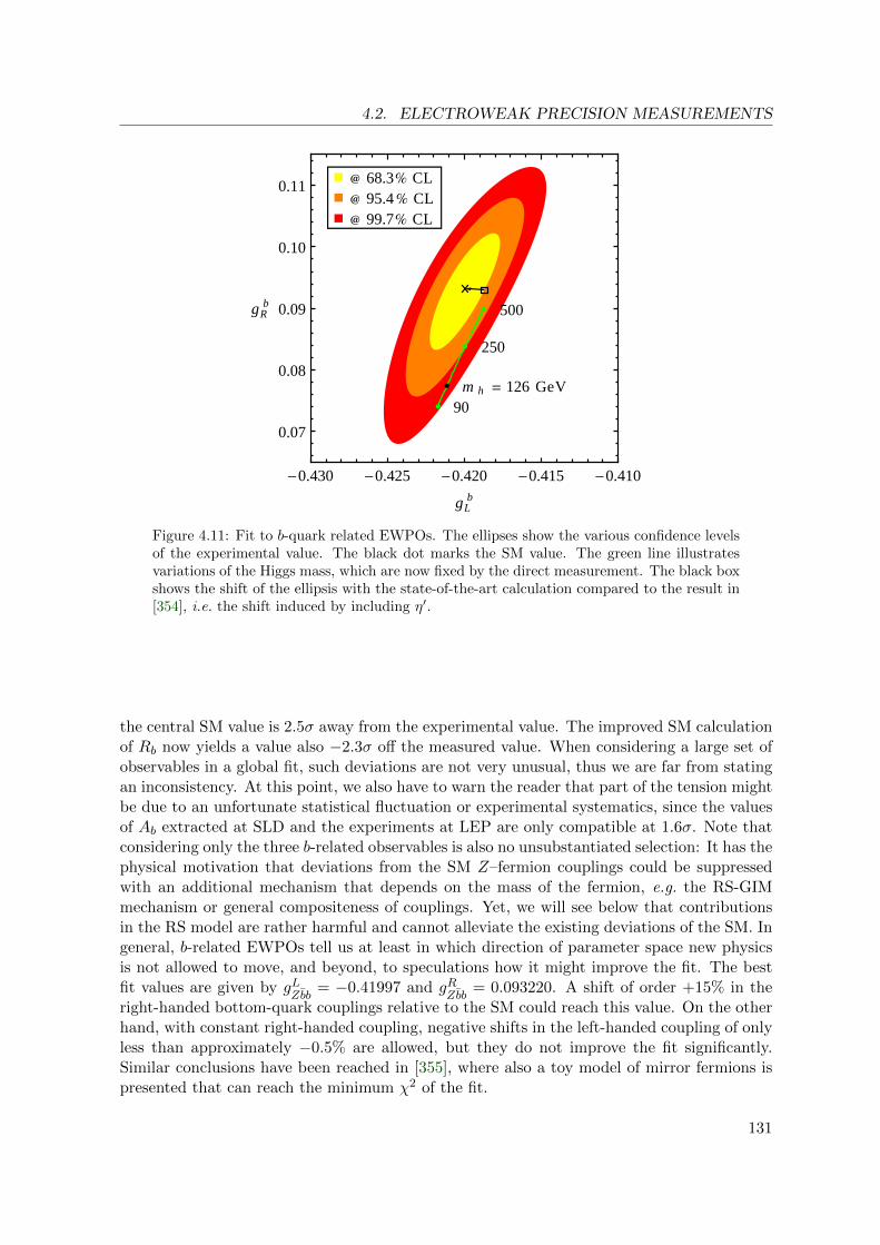
4.2. ELECTROWEAK PRECISION MEASUREMENTS
-0.430 -0.425 -0.420 -0.415 -0.410
0.07
0.08
0.09
0.10
0.11
gLb
gRb
90
250
500
mh = 126 GeV
68.3% CL 95.4 % CL 99.7% CL
Figure 4.11: Fit to b-quark related EWPOs. The ellipses show the various confidence levelsof the experimental value. The black dot marks the SM value. The green line illustratesvariations of the Higgs mass, which are now fixed by the direct measurement. The black boxshows the shift of the ellipsis with the state-of-the-art calculation compared to the result in[354], i.e. the shift induced by including η′.
the central SM value is 2.5σ away from the experimental value. The improved SM calculationof Rb now yields a value also −2.3σ off the measured value. When considering a large set ofobservables in a global fit, such deviations are not very unusual, thus we are far from statingan inconsistency. At this point, we also have to warn the reader that part of the tension mightbe due to an unfortunate statistical fluctuation or experimental systematics, since the valuesof Ab extracted at SLD and the experiments at LEP are only compatible at 1.6σ. Note thatconsidering only the three b-related observables is also no unsubstantiated selection: It has thephysical motivation that deviations from the SM Z–fermion couplings could be suppressedwith an additional mechanism that depends on the mass of the fermion, e.g. the RS-GIMmechanism or general compositeness of couplings. Yet, we will see below that contributionsin the RS model are rather harmful and cannot alleviate the existing deviations of the SM. Ingeneral, b-related EWPOs tell us at least in which direction of parameter space new physicsis not allowed to move, and beyond, to speculations how it might improve the fit. The bestfit values are given by gL
Zbb= −0.41997 and gR
Zbb= 0.093220. A shift of order +15% in the
right-handed bottom-quark couplings relative to the SM could reach this value. On the otherhand, with constant right-handed coupling, negative shifts in the left-handed coupling of onlyless than approximately −0.5% are allowed, but they do not improve the fit significantly.Similar conclusions have been reached in [355], where also a toy model of mirror fermions ispresented that can reach the minimum χ2 of the fit.
131
4. ASPECTS OF PRECISION PHYSICS
4.2.2 Constraints on the Randall-Sundrum Model
The leading effects on EWPOs in RS models arise already at tree-level and therefore havethe potential to be highly constraining. Thanks to the RS-GIM mechanism, we have seenin section 3.3.8.2 that the contributions for light fermions localized near the UV brane areuniversal to a large extent. In the following, we quantify the universal and the b-quark relatedconstraints in turn. We will discuss in detail how the custodial fermion embedding permitsto alleviate the bounds from EWPOs.
4.2.2.1 General Discussion and Input Parameters
We start with reviewing the input parameters. In the last section we have seen that universalmodifications of the couplings of the light fermions cancel in the asymmetries — as defined in(4.2.4) — making the effective weak angle sl 2eff a natural choice. At tree-level we can thereforesimply work with the value given in the last section for sl 2eff and s2
w. The shift in the on-shell definition s2
os and s20 are simple to work out, but we remark that their expressions are
modified by a term ∼ LM2W /M
2KK compared to the usual SM expression. The Fermi-constant
is affected by the universal shift. Extracting it from the charged-current four-fermion couplinggiven in (3.3.153) we obtain at O(v2/M2
KK)
GF√2
=g2
8M2W
[1 +
M2W
2M2KK
(1− 1
2L
)]. (4.2.18)
It is useful to maintain the definition of vSM in terms of GF and relate it to the Higgs VEVv that is necessary in the RS model to obtain the correct W -boson mass from (3.3.81). Weexpress this as [356]
κv ≡v
vSM= 1 +
M2W
4M2KK
(L
c2V
− 1 +1
2L
), (4.2.19)
which holds for the custodial RS model and for the minimal model with cV → 1.Concerning low energy EWPOs, it is interesting to note that a full 5d one-loop calculation
of the anomalous magnetic moment of the muon [231] finds a very small contribution, wellbelow the current uncertainty, even for MKK as low as 500 GeV.
4.2.2.2 Oblique and Universal Contributions
We summarize the oblique and universal contributions to the EWPOs with light fermionswith the S, T , and U parameters introduced in section 4.2.1.2. Following [187], we writethese in standard self-energy notation, despite the fact that the 5d contributions arise in factat tree level.
We calculated the non-zero tree-level correlators ΠV V (0) and Π′V V (0) with V = W,Z intwo ways. The simplest method is to use the zero-mode masses (3.3.81) and profiles (3.3.80)in order to calculate the modifications to the pure zero mode exchange. This corresponds tothe original on-shell definition of Peskin and Takeuchi. We obtain at O(v2/M2
KK)
Seff =2πv2
M2KK
(1− 1
L
), Teff =
πv2
2 c2wM
2KK
([ 1
c2Z
− c2w
c2W
] Ls2w
− 1
2L
), Ueff = 0 . (4.2.20)
As an alternative, yet more lengthy, check of the result we used the full 5d bosonic propagatorto derive S, T , and U in the definition of Barbieri et. al. [350]. This summarizes the full
132
4.2. ELECTROWEAK PRECISION MEASUREMENTS
contribution from all KK bosons, according to the approach of [350] to summarize all universal
corrections. To this end one c use Σ(k)V (t, t′) for k = 1 given in (3.3.102), in order to derive
ΠV V (0), and generalize the method to k = 2, 3 to obtain the derivatives of the vacuumpolarization. Here, we used instead the full gauge boson propagator for the minimal modelfrom [210]. Taking the version for euclidean momentum p0
E = −ip0 we obtain the vacuumpolarization and its derivatives as
ΠV V (pE) = −(L
kDV⊥µν (q; ε, ε)
)−1
− p2E −M2
V = ΠV V (0)− p2E Π′V V (0) +
p4E
2Π′′V V (0) . (4.2.21)
A straightforward calculation leads to
S =2πv2
M2KK
, T =πv2
2c2wM
2KK
L , W = Y =g2 v2
16M2KK L
, (4.2.22)
in agreement with [214, 357–359]. Relating this to the effective parameters via (4.2.8) weobtain the same result as before in (4.2.20) with cV = 1.
The result (4.2.20) clearly shows that custodial protection is automatically at work in thebreaking scheme where SU(2)L × SU(2)R is broken to the diagonal subgroup. We have seenin section 3.3.5.1 that this leads to the relation c2
Z = c2W /c
2w, canceling the L-enhanced term
in Teff . This holds irrespective of further details of the model, like e.g. the PLR symmetry.The minimal model holds with cW,Z → 1 such that Teff is larger by a factor of approximately2L2 ∼ 103 in the minimal model compared to the custodial model. We derive the followingnumerical constraints on the KK scale and first KK gluon excitation at 99.73% (3σ) CL
minimal RS: ε = 10−15, MKK > 4.6 TeV, MG(1) > 11.3 TeV,
custodial RS: ε = 10−15, MKK > 1.7 TeV, MG(1) > 4.1 TeV,
little RS: ε = 10−3, MKK > 1.8 TeV, MG(1) > 4.7 TeV.
(4.2.23)
The full dependence of the lower bound on the KK scale on the volume of the extra dimensionis shown in figure 4.12. There, and in the bounds given in (4.2.23), we take the uncertaintyon mt and Mh into account, allowing it to vary at the same CL like the S and T parameters.Almost all of the variation stems from the top-mass uncertainty. The full variation of thelower limit with the uncertainties is shown in the shaded bands in figure 4.12. Using themean values for mt and Mh, one would overestimate the bound on the minimal RS model in(4.2.23) by 13%. We observe that the LRS model [192] with small warp factor poses a viablealternative to the custodial protection in order to protect the T parameter. Of course onegives up the idea of connecting the weak scale with the scale of gravity but rather assumesnew phenomena to set in at an intermediate scale.
The limits on the custodial RS model stem almost entirely from the bound on S and areessentially independent of L. We see that the 68% CL limit on MKK is relatively high due tothe measurement being only compatible with the reference SM point at approximately this CL.The small negative shift in T from the custodial RS model cannot improve the fit. Rather onthe contrary, there might be harmful negative contributions to the T -parameter at loop-levelfor relatively light KK fermions. In [224, 360] the fermion contribution to the T parameteris found to be finite at one-loop level for a related fermion embedding in the context of anSO(5) gauge–Higgs-unification model. The presence of bidoublets — as introduced in section3.3.5.2 to embed the left-handed quark doublet in the extended SU(2)L × SU(2)R × U(1)X
133

4. ASPECTS OF PRECISION PHYSICS
10 15 20 25 30 35
2
3
4
5
6
7
8
L
MK
K@Te
VD
68.3% CL 95.4 % CL 99.7% CL
Figure 4.12: Constraints on the KK scale from S and T . The solid lines show the lowerlimit on the KK scale in dependence on the volume of the extra dimension L. The shadedbands indicate the uncertainty from mt and Mh. We include the uncertainty on mt andMh at the same CL like the constraint on S and T . The steep/flat lines are valid for theminimal/custodial model.
gauge group — is found to typically induce a negative shift in the T parameter. Obtainingvery light KK fermions (called custodians) is impossible with our fermion embedding, sincethe necessary bulk mass configuration requires strong PLR breaking. This leads to mixing intothe left-handed b quark, whose couplings to the Z boson are modified, but they are stronglyrestricted as we discuss below. Furthermore, the one-loop Higgs-sector contribution to theT -parameter has been found to be finite as well, but logarithmically UV divergent for theS parameter [223]. The authors of the latter reference find this result independently of themodel details. This could result in a large and positive S parameter. The numerical detailsof the one-loop corrections to S and T remain unquantified and are beyond the scope of thisthesis. Qualitatively, the discussion given here tells us that the bounds in (4.2.23) could beraised.
When one allows for more elaborate extra-dimensional model building and departuresfrom the minimal setups we consider here, then there exist of course methods to protect theT -parameter. One possibility uses large brane-localized kinetic terms for the gauge fields[357, 361, 362]. Since such terms are needed as counterterms to cancel divergences appearingat the loop level [363, 364], they are expected on general grounds to be present in an orbifoldtheory. The bare contributions to the brane-localized kinetic terms encode the unknown UVphysics at or above the cutoff scale. To retain the predictivity of the model, we assume thatthese bare contributions are small. As we concentrate on the leading contributions to theelectroweak precision observables, we furthermore ignore possible effects of brane-localizedkinetic terms appearing at the loop level. Even if these assumptions would be relaxed, thebound on the KK-gauge-boson masses that derives from the constraints on the S and Tparameters would remain anti-correlated with the mass of the Higgs boson. For example, the
134

4.2. ELECTROWEAK PRECISION MEASUREMENTS
authors of [362] found that having a light KK spectrum would require a value of the Higgsmass in the range of several hundred GeV. Another alternative direction of model building,which we did not discuss here, allows for variations of the 5d metric in the IR region. For therequired model building and details we refer to [365, 366].
4.2.2.3 Bounds from the Zbb Vertex
We continue with an analysis of the most important non-oblique correction, given by theprecision measurements of the Zbb vertex. To this end we derive approximate expressions forgLZbb
and gLZbb
in the ZMA (see section 3.3.6) and furthermore use relations following from aFroggatt-Nielsen analysis, i.e. corresponding to an expansion in the Cabibbo angle. Startingfrom the general expression for the couplings (3.3.142) we find to the order considered
gbZ,L =
(− 1
2+s2w
3
)[1− M2
Z
2M2KK
F 2(cbL)
3 + 2 cbL
(ωbLZ L−
5 + 2cbL2(3 + 2 cbL)
)]
+m2b
2M2KK
1
1− 2 cbR
(1
F 2(cbR)
[1− δc
1− 2 cbR1− 2 cb′R
]− 1 +
F 2(cbR)
3 + 2 cbR
)
+
2∑
i=1
|(Yd)3i|2|(Yd)33|2
1
1− 2 cdi
1
F 2(cbR)
[1− δc
1− 2 cdi1− 2 cd′i
], (4.2.24)
gbZ,R =s2w
3
[1− M2
Z
2M2KK
F 2(cbR)
3 + 2 cbR
(ωbRZ L− 5 + 2 cbR
2(3 + 2 cbR)
)]
− m2b
2M2KK
1
1− 2 cbL
(1
F 2(cbL)− 1 +
F 2(cbL)
3 + 2 cbL
)+
2∑
i=1
|(Yd)i3|2|(Yd)33|2
1
1− 2cQi
1
F 2(cbL)
,
where cbL ≡ cQ3 . In order to unify the notation of the custodial with the minimal model,we also write cdi ≡ cT2,i and cd′i ≡ cT1,i . The coefficient δc ∈ 0, 1 multiplies terms thatare only present in the custodial model. In these terms we assumed cd′i < 1/2, what is also
required for obtaining a sensible quark spectrum. Note that we use the bottom-quark MSmass mb ≡ mb(MKK) evaluated at the KK scale. On the other hand, the electromagneticcoupling and the weak mixing angle are running parameters in the low-energy EFT, which isobtained after decoupling the RS contributions at the scale MKK. We effectively include theassociated large logarithms by replacing s2
w(MKK) with s2w(mZ) in (4.2.24). We still allow for
cT1,i 6= cT2,i , i.e. PLR symmetry breaking by the triplet bulk masses, and retain the parameters
ωbLZ and ωbRZ . Remind that in the custodial embedding of section 3.3.5.2, we found ωbLZ = 0
and ωbRZ ≈ 10, while both factors are set to one in the minimal model.
From (4.2.24), we observe that the non-universal reduction of gbZ,R is in any case negativeand approximately 10 times more so in the custodial model. This direction of contributionsto gbZ,R is strongly constrained by the bottom-quark pseudo observables, as we have seen insection 4.2.1. We will see below, that this puts a mild upper bound on the size of cbR in thecustodial model, while the contributions are irrelevant in minimal model. The shift in gbL ispositive in the minimal model and almost absent in the model with custodial protection witha small negative contribution remaining. If one allows the PLR symmetry to be broken bycdi 6= cd′i , then the shift in gbL can also be positive in the custodial model as a result of fermion
135
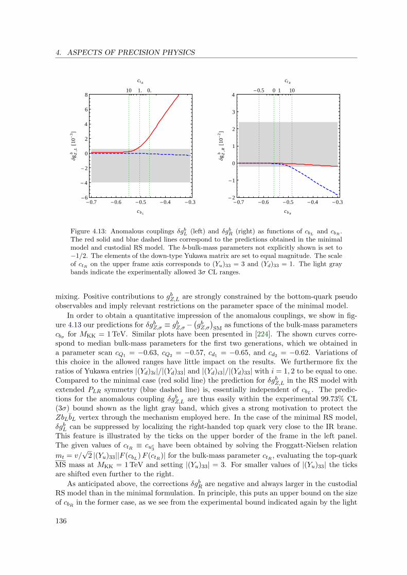
4. ASPECTS OF PRECISION PHYSICS
-0.7 -0.6 -0.5 -0.4 -0.3-6
- 4
- 2
0
2
4
6
80.1.10
cbL
∆gZ
,Lb
@10-
3D
ct R
-0.7 -0.6 -0.5 -0.4 -0.3- 2
-1
0
1
2
3
4-0.5 0 1 10
cbR
∆gZ
,Rb
@10-
2D
ct R
Figure 4.13: Anomalous couplings δgbL (left) and δgbR (right) as functions of cbL and cbR .The red solid and blue dashed lines correspond to the predictions obtained in the minimalmodel and custodial RS model. The b-bulk-mass parameters not explicitly shown is set to−1/2. The elements of the down-type Yukawa matrix are set to equal magnitude. The scaleof ctR on the upper frame axis corresponds to (Yu)33 = 3 and (Yd)33 = 1. The light graybands indicate the experimentally allowed 3σ CL ranges.
mixing. Positive contributions to gbZ,L are strongly constrained by the bottom-quark pseudoobservables and imply relevant restrictions on the parameter space of the minimal model.
In order to obtain a quantitative impression of the anomalous couplings, we show in fig-ure 4.13 our predictions for δgbZ,σ ≡ gbZ,σ−
(gbZ,σ
)SM
as functions of the bulk-mass parameterscbσ for MKK = 1 TeV. Similar plots have been presented in [224]. The shown curves corre-spond to median bulk-mass parameters for the first two generations, which we obtained ina parameter scan cQ1 = −0.63, cQ2 = −0.57, cd1 = −0.65, and cd2 = −0.62. Variations ofthis choice in the allowed ranges have little impact on the results. We furthermore fix theratios of Yukawa entries |(Yd)3i|/|(Yd)33| and |(Yd)i3|/|(Yd)33| with i = 1, 2 to be equal to one.Compared to the minimal case (red solid line) the prediction for δgbZ,L in the RS model withextended PLR symmetry (blue dashed line) is, essentially independent of cbL . The predic-tions for the anomalous coupling δgbZ,L are thus easily within the experimental 99.73% CL(3σ) bound shown as the light gray band, which gives a strong motivation to protect theZbLbL vertex through the mechanism employed here. In the case of the minimal RS model,δgbL can be suppressed by localizing the right-handed top quark very close to the IR brane.This feature is illustrated by the ticks on the upper border of the frame in the left panel.The given values of ctR ≡ cuc3 have been obtained by solving the Froggatt-Nielsen relation
mt = v/√
2 |(Yu)33||F (cbL)F (ctR)| for the bulk-mass parameter ctR , evaluating the top-quarkMS mass at MKK = 1 TeV and setting |(Yu)33| = 3. For smaller values of |(Yu)33| the ticksare shifted even further to the right.
As anticipated above, the corrections δgbR are negative and always larger in the custodialRS model than in the minimal formulation. In principle, this puts an upper bound on the sizeof cbR in the former case, as we see from the experimental bound indicated again by the light
136

4.2. ELECTROWEAK PRECISION MEASUREMENTS
gray band. Still, the ZbRbR coupling is predicted to be SM-like if we require to reproduce thelarge top-quark mass with Yukawa couplings of O(1). This can be inferred from the ticks onthe upper border of the frame in the right panel. They have been obtained by combining theFroggatt-Nielsen approximation mb = v/
√2 |(Yd)33||F (cbL)F (cbR)| with the one for mt given
earlier, solving again for ctR . The Yukawa parameters have been fixed to |(Yd)33| = 1 and|(Yu)33| = 3. For smaller values of |(Yd)33| the ticks move to the right and vice versa for largervalues. Rescaling |(Yu)33| has the opposite effect. With the choice of a bulk-mass parameternot exceeding the curvature scale14 ctR < 1, we observe that the bound is only relevant forvery low values of |(Yd)33|. This observation leads us to the conclusion that, irrespectivelyof the bulk gauge group, naturalness in combination with the requirement to reproduce theobserved top- and bottom-quark masses excludes large corrections to δgbR in models of warpedextra dimensions in which the left-handed bottom and top quark reside in the same multiplet.This model-independent conclusion should be contrasted with the analysis [367], which findssizable corrections in δgbR. The values of the bulk-mass parameters cbL,R and ctR consideredin the latter article lead to bottom- and top-quark masses of mb ≈ 40 GeV and mt ≈ 75 GeV,which are in conflict with observation. We finally remark that if the left-handed bottomand top quarks arise as an admixture of the zero-mode fields of two SU(2)L doublets, thenthe bottom- and top-quark masses are determined by two independent sets of bulk-massparameters, so that it is possible to account simultaneously for the quark masses and mixingsas well as the A0,b
FB anomaly [368].
The full impact of the constraints on the anomalous Zbb couplings on the relevant modelparameters are shown in figure 4.14 for the minimal, and figure 4.15 for the custodial RSmodel. The colored contours indicate the magnitude |(Yd)33| necessary to achieve the observedvalue of the bottom-quark mass. Requiring in addition a consistent value of the top quarkmass restricts the parameter space further. This is indicated by the cyan, dashed regions,which enclose the allowed range for allowed hierarchies in the Yukawa matrices between onefor the innermost and four for the outermost region.
In the case of the minimal model we illustrate with bright colors the importance of includ-ing the m2
b/M2KK corrections as opposed to the region with faint colors, where they are set
to zero. They originate from the term (δQ,q)33 in (3.3.142) that parametrizes singlet–doubletfermion mixing and contribute with a term that is proportional to F (cbL,R)−2. This term is
relevant for δgLZ,b, in which cbR enters. Consequently, the b-related EWPOs, pose a tight con-straint on the amount of UV localization of the right-handed b-quark. A similar constraintis also active in the custodial model when we break the PLR symmetry by the bulk-massparameters cb′R 6= cbR . In the case of full PLR symmetry the whole faintly colored regionof figure 4.15 is accessible. We demonstrate by the brightly colored region that the choicecb′R = 0 cuts away a relevant part of the parameter space for low values of MKK. Notice that
the main PLR breaking correction to gbL in (4.2.24) scales like −v2/M2KK |(Yd)33|2 F 2(cbL)
as seen from the aforementioned Froggatt-Nielsen approximation. This explains why values|(Yd)33| & 1 are not compatible with the Z → bb data in the case cb′R = 0.
Taking a completely random approach to the fundamental Yukawa and bulk-mass param-eters, we also did a numerical scan over the parameter space. We generated a large sampleof parameter points with viable quark spectrum and calculated the Zbb-couplings withoutresorting to the approximations used above. Further details on this parameter scan are de-scribed in appendix B.3. With the parameter scan, we can quantify the constraining power
14Remark that one also has to require ctR > −1/2 in order to reproduce the large top mass.
137

4. ASPECTS OF PRECISION PHYSICS
-0.6 -0.5 -0.4 -0.3-0.65
-0.60
-0.55
-0.50
-0.45
-0.40
-0.35
-0.30
cbL
c bR
MKK = 2 TeV
HYd L 33 = 0.25
0.5
12
4
-0.6 -0.5 -0.4 -0.3-0.65
-0.60
-0.55
-0.50
-0.45
-0.40
-0.35
-0.30
cbLc b
R
MKK = 4 TeV
Figure 4.14: 3σ CL in the cbL–cbR plane for the minimal RS model and MKK = 2 TeV andMKK = 4 TeV. The colored contours indicate the value of |(Yd)33| necessary to reproducethe value of the bottom-quark mass. The same color code is used in all plots. The brightcolors show the numerical result of the full expressions for gbZ,σ (4.2.24), while faint colors
indicate the result without terms proportional m2b/M
2KK. The dashed cyan lines enclose the
regions where top and bottom-quark mass can be reproduced with |ctR | < 1, and all Yukawaelements and ratios of Yukawa elements in the range [1/n, n], with n = 1, 2, 3, 4 for the foursuccessively larger regions.
-0.5 0.0 0.5 1.0-0.65
-0.60
-0.55
-0.50
-0.45
-0.40
-0.35
-0.30
cbL
c bR
MKK = 1 TeV
-0.5 0.0 0.5 1.0-0.65
-0.60
-0.55
-0.50
-0.45
-0.40
-0.35
-0.30
cbL
c bR
MKK = 2 TeV
Figure 4.15: 3σ CL in the cbL–cbR plane for the custodial RS model for MKK = 1 TeVand MKK = 2 TeV. Here the faint colors correspond to the full result (including m2
b/M2KK
terms) and active PLR symmetry cb′R = cbR . Only the brightly colored region is accessiblefor broken PLR symmetry with a fixed value of cb′R = 0. The remaining properties of theplot agree with figure 4.14
138
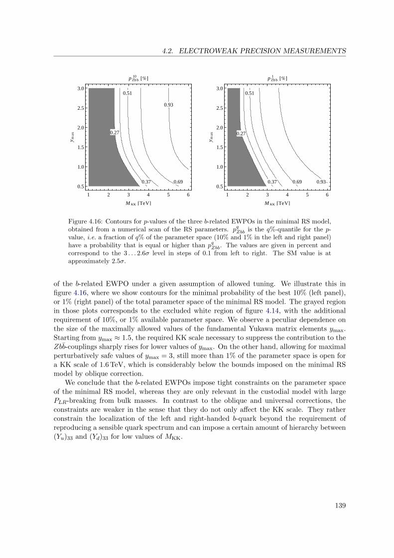
4.2. ELECTROWEAK PRECISION MEASUREMENTS
0.27
0.37
0.51
0.69
0.93
1 2 3 4 5 6
0.5
1.0
1.5
2.0
2.5
3.0
MKK @TeV D
y max
pZbb10 @%D
0.27
0.37
0.51
0.69 0.93
1 2 3 4 5 6
0.5
1.0
1.5
2.0
2.5
3.0
MKK @TeV Dy m
ax
pZbb1 @%D
Figure 4.16: Contours for p-values of the three b-related EWPOs in the minimal RS model,obtained from a numerical scan of the RS parameters. pqZbb is the q%-quantile for the p-value, i.e. a fraction of q% of the parameter space (10% and 1% in the left and right panel)have a probability that is equal or higher than pqZbb. The values are given in percent andcorrespond to the 3 . . . 2.6σ level in steps of 0.1 from left to right. The SM value is atapproximately 2.5σ.
of the b-related EWPO under a given assumption of allowed tuning. We illustrate this infigure 4.16, where we show contours for the minimal probability of the best 10% (left panel),or 1% (right panel) of the total parameter space of the minimal RS model. The grayed regionin those plots corresponds to the excluded white region of figure 4.14, with the additionalrequirement of 10%, or 1% available parameter space. We observe a peculiar dependence onthe size of the maximally allowed values of the fundamental Yukawa matrix elements ymax.Starting from ymax ≈ 1.5, the required KK scale necessary to suppress the contribution to theZbb-couplings sharply rises for lower values of ymax. On the other hand, allowing for maximalperturbatively safe values of ymax = 3, still more than 1% of the parameter space is open fora KK scale of 1.6 TeV, which is considerably below the bounds imposed on the minimal RSmodel by oblique correction.
We conclude that the b-related EWPOs impose tight constraints on the parameter spaceof the minimal RS model, whereas they are only relevant in the custodial model with largePLR-breaking from bulk masses. In contrast to the oblique and universal corrections, theconstraints are weaker in the sense that they do not only affect the KK scale. They ratherconstrain the localization of the left and right-handed b-quark beyond the requirement ofreproducing a sensible quark spectrum and can impose a certain amount of hierarchy between(Yu)33 and (Yd)33 for low values of MKK.
139

4. ASPECTS OF PRECISION PHYSICS
4.3 Higgs Production and Decays at Hadron Colliders
The remainder of this thesis is devoted to the topic of Higgs production and decays. Since suchprocesses were only very recently measured for the first time, the subject is in a major upheavalperiod from the experimental point of view. This implies that Higgs processes will soonconstitute a third pillar of precision constraints on models beyond the SM. On the theoreticaland phenomenological side, the physics behind these processes is well understood and precisepredictions can be made for the SM. Also beyond the SM, the effects of additional particlesare well understood for perturbatively unitary theories like the minimal supersymmetric SM,general two-Higgs-doublet models, and left–right symmetric models. For reviews on Higgsphenomenology in these models see [106, 369, 370] and the references therein. Here, weinvestigate the effect of specific composite models. First, we review the SM results, theexperimental status, and contributions from partner fermions in the simple example of theLHT model. Our main focus is then to determine the analytical and numerical structure ofthe effects in the RS model, discuss the subtle issue of convergence of loop integrals, and thepotential to constrain the parameter space.
4.3.1 Results in the SM and Measurements
With the recent discovery of a bosonic resonance [22, 29, 41] that is presumably due to theHiggs boson15, we entered a new era of particle physics. Since apart from the resonance massMh ≈ 126 GeV also the first bounds on its couplings were obtained, Higgs physics has reacheda turning point in making the transition from discovery to precision physics.
The couplings of the Higgs boson to fermions and gauge bosons have a peculiar structurein the SM. This originates in the simple mechanism of electroweak symmetry breaking. Thecouplings of the Higgs boson to gauge bosons are obtained from covariant derivatives, whilstfermions couple to the Higgs boson via Yukawa couplings. Since these terms are the onlysources of all particle masses and there is only a single scalar direction that takes a VEV,the corresponding couplings of the physical Higgs boson are directly proportional the samemass. Decay widths to heavy particles are consequently enhanced compared to those intolight particles. The same is true for the production of the Higgs boson: Direct Higgs-bosoncouplings of the light quarks contained in protons, or of electrons in the initial state contributeto production to a negligible extent. Thus, the main production channels we must considereither involve heavy quarks, most importantly the top quark, or heavy gauge bosons.
For hadron colliders, such as the Tevatron and the LHC, the main production process isdue to fusion of two gluons. The leading order (LO) Feynman diagram is depicted in theupper left panel of figure 4.17. Since this process is particularly interesting in the modelsof new physics we discuss below, we will review it in some detail before commenting on theother production modes.
We take a closer look at the on-shell amplitude for the diagram depicted in the upper left
15Since the discovered particle decays also into two photons it must be a boson. The Landau-Yang theorem[371, 372] implies that it cannot be of spin 1. Evidence for the decay into Z bosons suggests that it participatesin electroweak symmetry breaking. Recent measurements of ATLAS [27] and CMS [36] already disfavor thepseudo-scalar and spin two hypothesis roughly at the level of one percent. For simplicity we call the observedresonance the Higgs boson.
140

4.3. HIGGS PRODUCTION AND DECAYS AT HADRON COLLIDERS
Q
Q
Q
g
g
hQ
Q
g
g
Q
h
Q
V ∗
q V
hq
V ∗
V ∗
q
q
q
h
q
Figure 4.17: Feynman diagrams for the leading order contributions to the dominant Higgsproduction mechanisms in the SM at hadron colliders. For the subleading production withheavy quarks in the upper right panel there are additional tree-level diagrams with the Higgsboson attached to other lines, with a trilinear gluon coupling, and with qq initial state.
panel of figure 4.17. After evaluating the fermionic trace it is given by
M(gg → h
)= 2i
g2s m
2q
vδab εµ(p) εν(q)
× µ2ε
∫dDk
(2π)D
gµν(m2q −M2
h/2− k2)
+ 4kµkν + qµpν
(k2 −m2
q
)[(k + p
)2 −m2q
][(k − q
)2 −m2q
] ,(4.3.1)
where mq is the mass of the internal fermion. The momentum p, Lorentz-index µ, and color-index a belong to one gluon and q, ν, b to the other. We have already written the expressionusing dimensional regularization in D = 4 − 2ε dimensions, even though we know the loop-integral must be finite because of renormalizability of the SM. However, a gauge invariantregulator is necessary to obtain the correct finite result, which fulfills the Ward identities.They require the amplitude to be proportional to qµpν − gµνM2
h/2. One can indeed observea curious cancellation of two specific finite terms. We rewrite the loop-integral in the secondline of (4.3.1) with the conventional three-point functions, defined e.g. in [373], to obtain
i
(4π)2
(Cρσ(p2, q2;mq,mq,mq)
(4gµρgνσ − gµνgρσ
)
+ C0(p2, q2;mq,mq,mq)(gµν[m2q −M2
h/2]
+ qµpν)).
(4.3.2)
Reducing the tensor function Cρσ with the Passarino-Veltman method [374] one sees thatit contains a contributions from a scalar two point functions gρσB0(p;mq,mq). The 1/εdivergence in B0 is however multiplied with a Lorentz structure from the fermion trace thatwould vanish in D = 4 given by
(4gµρgνσ − gµνgρσ
)gρσ = 2εgµν . This leads to a finite,
non-gauge invariant term which cancels against the non-gauge invariant terms in the secondline of (4.3.2). The necessity of a proper regularization is a crucial observation that we alsoencounter in the 5-dimensional calculation in the RS model in section 4.3.3. However, theargument is of different nature in that model. Instead of the breakdown of gauge invariance
141

4. ASPECTS OF PRECISION PHYSICS
we observe a resonance phenomenon at an artificial physical scale that is inexistent when thetheory is properly UV-regularized.
The amplitude for gg → h can finally be written as [375]
M(gg → h
)=
αs3πv
δabεµ(p)εν(q)
(gµν
M2h
2− qµpν
)Ahq (τq) ,
Ahq (τ) = 3
1∫
0
dx
1−x∫
0
dy
(1− 4xy
1− 4xy/τ
), τq =
4m2q
M2h
− iε ,(4.3.3)
where we included a factor 2 to account for the diagram with crossed gluon lines. Up toprefactors, the result is encoded in the function Ahq (τq) and often called form factor in thiscontext. The form factors of all processes relevant for our discussion are compiled in appendixB.1. We observe that in the limit τq 1 we obtain Ahq (τq) = −3/8τq(ln(4τq) + iπ)2. Thisdirectly shows the marginal relevance of light quarks. The final partonic cross section is givenby
σ(gg → h) =α2sM
2h
576πv2
∣∣∣∑
q
Ahq (τq)∣∣∣2δ(s−M2
h) , (4.3.4)
with the partonic center of mass energy s. To obtain the hadronic cross section it has to befolded with the gluon luminosity involving appropriate parton distribution functions (PDF).In the narrow-width approximation, one considers the Higgs boson as a stable particle andneglects interference effects with background and other channels by employing the δ-functionin (4.3.4). This treatment is appropriate for a light Higgs mass as shown below in figure 4.19.The luminosity integral thus becomes a simple multiplication at leading order and for allvirtual corrections at higher orders. Consequently, the involved uncertainties drop out toa large extent, if we consider ratios of processes with different final states [376]. This isimportant, for accessing the coupling structure of the Higgs boson. We discuss this in moredetail below.
The largest contribution to the amplitude comes from the triangle diagram with internaltop quarks. It can be described by an effective operator of mass dimension 5 that arisesfrom integrating out the top quark16. The most general effective Lagrangian, on which thiscontribution is to be matched, reads
Leffggh = C1(µ)
αs(µ)
12π
h
vGaµν G
µν,a − C5(µ)αs(µ)
8π
h
vGaµν G
µν,a , (4.3.5)
where Gaµν is the gluon field strength tensor and µ ≤ mt is the scale at which the effectiveoperators are renormalized. We also included a CP -violating operator that involves the dualfield strength tensor Gµν,a = −1
2εµνρσ Gaρσ (with ε0123 = −1). It could be generated by pseudo-
scalar couplings from new physics but is zero in the SM. The Wilson coefficients are thus givenby C1(µ) = Ahq (mt) and C5(µ) = 0. We discuss the evolution of the Wilson coefficients in thenext section.
We can furthermore approximate the result using the limit of a heavy top mass. With ournormalization Ahq (τ) → 1 for τ → ∞. The resulting effective ggh coupling stays finite evenafter decoupling the top quark. This behavior stems from the top Yukawa coupling that isincluded in the form factor Ahq ∼ yt/v. In fact, there exists no physical decoupling limit which
16Interestingly this description is even valid for Mh > mt. See [377] for a didactic explanation.
142

4.3. HIGGS PRODUCTION AND DECAYS AT HADRON COLLIDERS
takes only the quark masses to infinity. The limit v →∞ would uniformly rescale the whole
spectrum, thereby violating the low energy constraint v =(√
2GµF)−1/2 ≈ 246GeV.17 This
justifies the non-decoupling of heavy chiral fermions, and the same reasoning also appliesto any possible fermions of new physics that receive their masses purely from electroweaksymmetry breaking.
The large mt approximation is very useful for the derivation of a specific low-energytheorem [378–380]. This theorem relates the given amplitude with one external Higgs bosonto such amplitudes with no, or more than one Higgs boson in the heavy mt limit. Foramplitudes with more than one Higgs boson this is easily seen by inserting an additional toppropagator and a Yukawa coupling in the diagram, what leads to the replacement
1
/k −mt−→ 1
/k −mt
mt
v
1
/k −mt=mt
v
∂
∂mt
1
/k −mt. (4.3.6)
The general low-energy theorem is the intuitive generalization of this recipe
limph→0
M(I → F + h) =∑
q
λhqmq
v
∂
∂mqM(I → F) . (4.3.7)
M is the matrix element for any initial state I, a final state F that may already contain Higgsbosons, and a generalized sum over fermions of bare mass mq in the loop. The vanishing Higgsmomentum on the left-hand side is equivalent to taking the large mq limit, since the massinside the loop cannot be resolved by the external momentum. The sum (4.3.7) is alreadysuitable for more general chiral quarks by including the factor λhq that is equal to one onlyin the SM. Already for a Higgs sector with more than one doublet those factors are givenin terms of mixing angles of the extended scalar sector [380]. Apart from the possibility tocalculate multi-Higgs production with (4.3.7), the relation also directly relates the large mt
limit of the ggh amplitude to the QCD β-function. This provides the possibility to calculatethe ggh amplitude at all orders from gluon self energies. On the right-hand side of equation(4.3.7), one only has to account for the renormalization of the bare masses by dividing bya factor 1 + γmq , with the mass anomalous dimension γmq . This results in the approximatenext-to-leading order (NLO) result of the SM
Leffggh =
αs(µ)
12π
βts4αs(1 + γm)
h
vGaµν G
µν,a
=αs(µ)
12π
(1 +
αs(µ)
4π(5Nc − 3CF ) +O(α2
s)
)h
vGaµν G
µν,a .
(4.3.8)
where βts is the top-quark contribution to the QCD β-function, Nc = 3 the number of colors,and CF = (N2
c − 1)/(2Nc) the quadratic Casimir operator. Remarkably, the accuracy of thelarge mt approximation is very high for Mh < 300 GeV, better than 1% compared to the fullmt dependence even at next-to-next-to-leading order (NNLO) [381]. In [237] the authors haveused (4.3.7) to derive a very general expression for C1 in models of new physics and relatethe sign of the shift in C1 to the cancellation of the quadratic divergence in the Higgs massin various scenarios of new physics.
17Infinite quark masses at fixed v require Yukawa couplings to enter the strong coupling regime, in whichperturbative arguments fail to apply.
143

4. ASPECTS OF PRECISION PHYSICS
100 200 300 400 5000.1
1
10
100
mh @ GeV D
Σ@p
bD
gg ®h
qq ¢ ® qq ¢ h
LHC s = 10 TeV
100 150 200 250 3000.001
0.01
0.1
1
10
mh @ GeV D
Σ@p
bD gg ®h
q q ®Wh
Tevatron s = 1.96 TeV
Figure 4.18: The two dominant production cross sections at center of mass energies relevantfor the LHC at 10 TeV (left) and the Tevatron at 1.96 TeV (right). The upper red lineshows the gluon–gluon fusion mode. The lower blue line shows weak gauge boson bosonfusion for the LHC and associated production with W for the Tevatron. For uncertaintiessee comments in the main text.
Beyond the top quark, also the bottom-quark contribution has to be taken into account.Numerically, it suffices to very good accuracy to multiply the final cross section σ(gg → h)without the bottom-quark corrections by a factor
(1+2 ReAhb
). This approximate treatment
decreases the cross section by about 9%, 2%, and less than 1% for Mh = 100 GeV, 300 GeV,and 600 GeV, in good agreement with the NLO calculation including the exact mass depen-dence [382–384].
Note that higher-order QCD corrections to the gluon–gluon fusion process are very impor-tant. At the LHC they increase the LO cross section by about 80-100% at NLO, by about 25%at NNLO [385–387], and another 6-9% stem from the resummation of soft gluons at NNLL.The current state of the art, including electroweak corrections, detector acceptances, and cutson differential distributions is compiled by the LHC Higgs Cross Section Working Group Col-laboration in [388, 389]. We should also account for QCD corrections when integrating outheavy colored particles in models of new physics in the following sections. For extra quarks,which have the same SU(3)c quantum number as the SM quarks, the QCD corrections arevery similar to those from integrating out the SM top quark. Like for the top quark, thegeneralization of (4.3.8) involves only the QCD β-function and mass anomalous dimension,which solely depend on the SU(3)c representation in a mass independent renormalizationscheme.
We show numerical values for the Higgs-production cross sections at the LHC and Tevatronfor center-of-mass energies
√s = 10 TeV and
√s = 1.96 TeV in figure 4.18. There we employ
the calculation of σ(gg → h) given in [390], which combines the next-to-next-to-leadingfixed-order corrections [385–387] with resummation of both threshold logarithms from soft-gluon emission [391–395] and terms of the form (Ncπαs)
n, which have been identified aspart of the source of large perturbative corrections [396]. The result is depicted in the redcurves of figure 4.18, where the MRST2006NNLO PDFs [397] and the associated normalizationαs(mZ) = 0.1191 for the strong coupling constant are used. The choice of low-energy input inthe form of different sets of PDFs introduces a major theoretical uncertainty. Furthermore,there is the issue how renormalization and factorization scale choices reflect the uncertaintyrelated to the truncation of the perturbative series. The total theoretical accuracy [388] is atthe level of 20%, on which the recent experimental precision is already closing in [22, 29].
144

4.3. HIGGS PRODUCTION AND DECAYS AT HADRON COLLIDERS
100 500200 300150
0.01
0.1
1
10
100
Mh @ GeV D
Gh
@GeV
D
Figure 4.19: Total width of the SM-Higgs boson. Both axes have a logarithmic scale.
Besides gluon–gluon fusion there are two main production processes mediated by weakgauge bosons, whose LO diagrams are depicted in the bottom row of figure 4.17. This isthe associated production with W/Z bosons [116, 398], which is the relevant productionchannel for the pp collisions at Tevatron, and the weak vector boson fusion processes [399,400], which is a subleading contribution at the LHC. Their total cross sections in hadroniccollisions is approximately 10 times lower than the gluon fusion cross section in the relevantHiggs-mass range, as depicted by the blue curves [401] in figure 4.18. Nevertheless, theyprovide an additional hadronic probe that allows to distinguish them from the overall hadronicbackground. For weak vector boson fusion the probes can be enhanced collinear forward jetsin a back-to-back geometry [402], which provide a very efficient cut against QCD backgrounds.Moreover, the QCD uncertainty of the theory prediction is much lower than in gluon–gluonfusion and the dominant, remnant PDF uncertainty stays below 3% in the relevant Higgs-massrange [388].
An additional, subleading, but experimentally important production mode is the associ-ated Higgs production with two heavy top [403, 404] or bottom [405, 406] quarks. Consideredwith a subsequent decay h→ bb it will play an important role in later stages of the LHC pro-gram as it allows to directly measure the top–Higgs coupling and constrain the bottom–Higgscoupling in supersymmetric models with large tan(β). For the plethora of other suppressedproduction processes, e.g. with one or more hard jets in the final state, double-Higgs produc-tion, diffractive production, etc. , we refer to [142] and references therein.
After production of the Higgs particle we can separately consider its subsequent decaywidths. As mentioned above, it couples to all particles, including itself, proportional to theparticles masses. The total width of the SM-Higgs boson shown in figure 4.19 is thereforedominated by the decay into the heaviest states allowed by phase space, which is eitherbb below, or W+W− above the W+W− threshold. The width increases drastically at thistransition. For the relevant low Higgs mass range we have already discussed that the narrowwidth approximation is suitable.
The past successive reduction of the allowed mass region [407–410] shows that a detectionof the Higgs boson at a mass of Mh ≈ 126 GeV has been difficult, particularly comparedto higher values of the Higgs mass, where the golden channel h → Z(∗)Z(∗) → 2l+2l− withthe experimentally clear leptonic final state would have allowed for real intermediate config-urations of the two Z bosons. The dominant decay into bottom-quark pairs is difficult toaccess if originating from gluon–gluon fusion, since the QCD background of bb production is
145
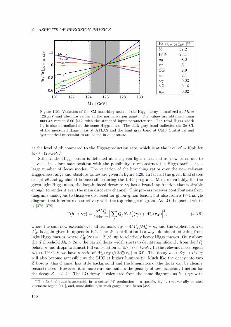
4. ASPECTS OF PRECISION PHYSICS
120 122 124 126 128 130
0.6
0.8
1.0
1.2
Mh @ GeV D
BrB
rM
h=
126
GeV bb, cc
WW
ggΤΤ , ΜΜ
ZZ
ΓΓ
ΓZ
G h
Br|Mh=126 GeV [%]
bb 57.2WW 23.1gg 8.2ττ 6.1ZZ 2.9cc 2.1γγ 0.23γZ 0.16µµ 0.02
Figure 4.20: Variation of the SM branching ratios of the Higgs decay normalized at Mh =126 GeV and absolute values at the normalization point. The values are obtained usingHDECAY version 5.00 [412] with the standard input parameter set. The total Higgs widthΓh is also normalized at the same Higgs mass. The dark gray band indicates the 3σ CLof the measured Higgs mass at ATLAS and the faint gray band at CMS. Statistical andsystematical uncertainties are added in quadrature.
at the level of µb compared to the Higgs-production rate, which is at the level of ∼ 10pb forMh ≈ 126 GeV.18
Still, as the Higgs boson is detected at the given light mass, nature now turns out toleave us in a fortunate position with the possibility to reconstruct the Higgs particle in alarge number of decay modes. The variation of the branching ratios over the now relevantHiggs-mass range and absolute values are given in figure 4.20. In fact all the given final statesexcept cc and gg should be accessible during the LHC program. Most remarkably, for thegiven light Higgs mass, the loop-induced decay to γγ has a branching fraction that is sizableenough to render it even the main discovery channel. This process receives contributions fromdiagrams analogous to those we discussed for gluon–gluon fusion, but also from a W -trianglediagram that interferes destructively with the top-triangle diagram. At LO the partial widthis [378, 379]
Γ(h→ γγ
)=
α2M3h
144π3v2
∣∣∣∑
f
QfNcAhq (τf ) +AhW (τW )
∣∣∣2, (4.3.9)
where the sum now extends over all fermions, τW = 4M2W /M
2h − iε, and the explicit form of
AhW is again given in appendix B.1. The W contribution is always dominant, starting fromlight Higgs masses, where AhW (∞) = −21/3, up to relatively heavy Higgs masses. Only abovethe tt threshold Mh > 2mt, the partial decay width starts to deviate significantly from the M3
h
behavior and drops to almost full cancellation at Mh ≈ 650 GeV. In the relevant mass regionMh ≈ 126 GeV we have a ratio of AhW (τW )/(2Ahq (τt)) ≈ 3.0. The decay h → Zγ → l+l−γwill also become accessible at the LHC at higher luminosity. Much like the decay into twoZ bosons, this channel has little background and the kinematics of the decay can be cleanlyreconstructed. However, it is more rare and suffers the penalty of low branching fraction forthe decay Z → l+l−. The LO decay is calculated from the same diagrams as h → γγ with
18The bb final state is accessible in associated W production in a specific, highly transversally boostedkinematic region [411], and, more difficult, in weak gauge boson fusion [388].
146
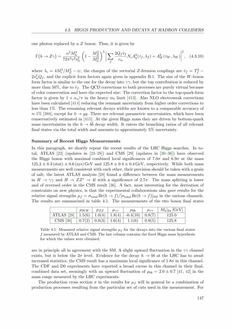
4.3. HIGGS PRODUCTION AND DECAYS AT HADRON COLLIDERS
one photon replaced by a Z boson. Thus, it is given by
Γ(h→ Zγ
)=
α2M3h
72π2v2s2w
(1− M2
Z
M2h
)3 ∣∣∣∣∑
f
2Qf vfcw
NcAhq (τf , λf ) +AhW (τW , λW )
∣∣∣∣2
, (4.3.10)
where λi = 4M2i /M
2Z − iε, the charges of the vectorial Z-fermion couplings are vf = T 3
f −2s2wQf , and the explicit form factors again given in appendix B.1. The size of the W -boson
form factor is similar to the one for the decay into γγ, but the top contribution is reduced bymore than 50%, due to vf . The QCD corrections to both processes are purely virtual becauseof color conservation and have the expected size: The correction factor to the top-quark-formfactor is given by 1 + αs/π in the heavy mt limit [413]. Also NLO electroweak correctionshave been calculated [414] reducing the remnant uncertainty from higher order corrections toless than 1%. The remaining relevant decays widths are known to a comparable accuracy of≈ 1% [388], except for h→ gg. There are relevant parametric uncertainties, which have beenconservatively estimated in [415]. At the given Higgs mass they are driven by bottom-quarkmass uncertainties in the h → bb decay width. It enters the branching ratios of all relevantfinal states via the total width and amounts to approximately 5% uncertainty.
Summary of Recent Higgs Measurements
In this paragraph, we shortly repeat the recent results of the LHC Higgs searches. In to-tal, ATLAS [22] (updates in [23–28]) and CMS [29] (updates in [30–36]) have observedthe Higgs boson with maximal combined local significances of 7.0σ and 6.9σ at the mass125.2 ± 0.3 (stat) ± 0.6 (sys) GeV and 125.8 ± 0.4 ± 0.4 GeV, respectively. While both massmeasurements are well consistent with each other, their precision should be taken with a grainof salt; the latest ATLAS analysis [28] found a difference between the mass measurementsin H → γγ and H → ZZ∗ → 4l with a significance of 2.7σ. The mass splitting is lowerand of reversed order in the CMS result [36]. A fact, most interesting for the derivation ofconstraints on new physics, is that the experimental collaborations also gave results for therelative signal strengths µf = σtotal Br(h → f)/[σtotal Br(h → f)]SM in the various channels.The results are summarized in table 4.1. The measurements of the two boson final states
µWW µZZ µγγ µbb µττ Mh|fix [GeV]
ATLAS [28] 1.5(6) 1.0(4) 1.8(4) -0.4(10) 0.8(7) 125.0
CMS [36] 0.7(2) 0.8(3) 1.6(4) 1.1(6) 0.9(5) 125.8
Table 4.1: Measured relative signal strengths µf for the decays into the various final statesf measured by ATLAS and CMS. The last column contains the fixed Higgs mass hypothesisfor which the values were obtained.
are in principle all in agreement with the SM. A slight upward fluctuation in the γγ channelexists, but is below the 2σ level. Evidence for the decay h → bb at the LHC has to awaitincreased statistics; the CMS result has a maximum local significance of 1.8σ in this channel.The CDF and D0 experiments have reported a broad excess in this channel in their final,combined data set, seemingly with an upward fluctuation of µbb = 2.0 ± 0.7 [41, 42] in themass range measured by the LHC experiments.
The production cross section σ in the results for µf will in general be a combination ofproduction processes resulting from the particular set of cuts used in the measurement. For
147

4. ASPECTS OF PRECISION PHYSICS
the comparison with theories of new physics an unfolding of the different production channelsis necessary. The experimental collaborations have partially provided the result for specifictags of the final state. Interestingly, in the CMS result, the enhanced central value of µγγ isonly present in the channel where a tag for vector boson related production was applied, whilethe central value for the combination of gluon–gluon fusion and associated top productionwas found to be marginally below one. On the other hand, no enhancement was found for thethe WW and ZZ final state with a vector boson related tag. A precise unfolding procedurefor the production modes is beyond the scope of this thesis. Below we will comment if ourconclusions are limited by this partial knowledge. At present this restriction is not yet veryrelevant, but will become so in the future. We refer to the very recent analyses [416, 417]where the unfolding based on simplifying assumptions was attempted in order to improvelimits on deviations from the SM.
4.3.2 Sensitivity of Higgs Production to New Fermions
In the last section we discussed the effective Lagrangian obtained by integrating out the topquark (4.3.5). Analogously, also contributions to the amplitude from heavy chiral fermionsbeyond the SM have the same non-decoupling behavior. In fact, the constant form factor inthe limit of large fermion masses implies a counting of heavy chiral fermions. This is veryrelevant for the model with a simple sequential fourth fermion generation (SM4). This modelwas already cornered from bounds of several sources. On the one hand, unitarity of thepartial S-wave amplitude for color-singlet, elastic, same-helicity t′t′ scattering at tree levelleads to a bound of mt′ . 500 GeV [139]. On the other hand, direct searches for decays ofheavy quarks at LHC lead to the bounds mb′ > 495 GeV [418] and mt′ > 656 GeV [419] at95% CL, and EWPOs also strongly restrict the up–down and lepton–neutrino mass splittings[420, 421] and further mixing parameters of this simple extension of the SM. The recentmeasurements of Higgs decays at the LHC have led to the final exclusion of the SM4 (withoutmodified Higgs sector) at the level of approximately 5σ [422]. Two main effects in the Higgsprocesses can be identified. The Higgs-production cross section via gluon–gluon fusion issimply enhanced by a factor of approximately 9 due to the additional t′ and b′-quarks in theloop [420]. Thus, a strong enhancement of τ+τ− events is also expected. On the contrary,extra loop-contributions of chiral fermions add constructively to the top-contribution in theamplitude of the decay h→ γγ and thus increase the cancellation of the W -boson loop [423],which leads to an overcompensation of the enhanced production.
The sensitivity of Higgs processes is of course less dramatic, or even inexistent, in modelswhere new fermions enter in vector-like form, i.e. with the same gauge-group representationsfor both chiralities, as they may obtain a TeV scale mass mainly from an explicit mass term.This is the case in the LHT model of section 3.2, where one parametrizes the strong dynamicsthat leads to the explicit mass by an additional input parameter λ+ (3.2.23). In the RSmodel, which we presented in section 3.3, mass terms arise in the form of eigenvalues for themomenta in the direction of a compact extra dimension.
Before entering the conceptually demanding calculation of loop processes for Higgs physicsin the RS model, it is instructive to reconsider the main aspects in the LHT model. A usefulparametrization became widely used recently. It is particularly suitable to categorize thetypical contributions of models in which the Higgs arises as a pseudo Nambu-Goldstone bosonin the framework of an EFT. The low-energy effective Lagrangian of the leading dimension-sixoperators [424] has been used as a basis for a matching of typical little Higgs models in [166].
148

4.3. HIGGS PRODUCTION AND DECAYS AT HADRON COLLIDERS
They find that in the LHT model, the coefficient of the effective operator |∂µ(Φ†Φ)|2/(2f2)is given by cH = 1/6. Its only source is the non-linearity of the NLσM, which changesthe standard relation between the W -boson mass and the Higgs VEV and can be read off(3.2.11).19 For the RS model we expressed the analogous shift with definition of a modifiedHiggs VEV (4.2.19).
As we have seen in section 3.2, the vector-like state t′+ then mixes under electroweaksymmetry breaking with the SM-like up-quarks and thus obtains also couplings to the Higgsboson, while the T -parity odd combination t′− remains unmixed. The effect of the modifiedtop-coupling and the heavy mass eigenstate T+ can be elegantly calculated from the low-energy theorem that lead to (4.3.8). This was observed in [237] and the argument goesas follows. The leading logarithmic contribution to the QCD β-function that stems fromintegrating out a heavy particle at the scale µ can in general be written as
1
g2s,eff(µ,H)
=1
gs(µ)2− b tr
4π2ln
(m(H)
µ
), (4.3.11)
where m(H) is the coupling that determines the particles mass once H = v+h is inserted, tris the Dynkin index of the representation and b = 2/3 for Dirac fermions and 1/6 for scalars.Here we only discuss the example of an additional fermion in the fundamental representation,tr = 1/2, but the applicability of the strategy is more general. The linearization in v andapplication of the low-energy theorem leads to the modified one-loop Wilson coefficient [166]
C1 =∑
i
∂ ln(mi(v))
∂ ln(v)
∣∣∣v=vSM
− cH2
v2SM
f2
=v
2
∂
∂vln det(M†(v)M(v))
∣∣v=vSM
− cH2
v2SM
f2,
(4.3.12)
where mi(v) summarizes the masses of the top quark and heavy top partners, like the T+.Furthermore, all form factors have been set to one, and all particles are integrated out at thesame scale. In this approximation we see that there is no need to diagonalize the mass matrix,and one only needs the determinant of the squared mass matrix M(v) of the top quark andtop partners in the gauge eigenstate basis. Using the lower-right 2× 2 sub-block of the massmatrix (3.2.24) one directly finds to O
(v2/f2
)
v
2
∂
∂vln det(M†M)
∣∣v=vSM
= 1− 2
3
v2SM
f2−→ CLHT, even
1 = 1− 3
4
v2SM
f2, (4.3.13)
in agreement with [166]. With f & 500 GeV being allowed from limits on ∆F = 2 FCNCs[163], the reduction could reach approximately −35% in the ratio of cross sections; 11% ofthis are due to the modified VEV.
In [166], mirror masses have been realized with a coupling to additional scalar fields X. Inthis way the mirror fermions do not couple directly to the Higgs boson and do not contributeto the Higgs processes at leading order. We abbreviate this model as LHTX. The contributionsfrom the traditional mirror mass terms, which we presented in (3.2.20), were calculated in[425]. We find from the couplings in (A.2.8) that
v ghfH,ifH,i
mfH,i
= −v2SM
4f2
v ghttmt
, (f = u, ν) , (4.3.14)
19The additional effects from gauge-boson mixing for g 6= g′ and a non-vanishing triplet VEV in the LHTmodel can be read off the same mass formula (3.2.11).
149

4. ASPECTS OF PRECISION PHYSICS
and vanishing Higgs coupling to down-type and lepton mirror quarks. For production viagluon–gluon fusion this implies a total modification from the T -odd sector, of the same sizelike from the T -even sector
CLHT, odd1 = −3
4
v2SM
f2. (4.3.15)
This agrees with the result in [425]. Within the used approximations, there exists no depen-dence on the mirror mass values. In particular, the mirror-fermion contribution cannot be sep-arately decoupled due to (4.3.14). Interestingly, precisely the same reductions were found inminimal composite Higgs models (MCHM), which are similar models based on SO(5)/SO(4)[426]. With both, the top being part of a full representation 5 or 10 of SO(5), one obtains
the same result CMCHM51 = CMCHM10
1 = CLHT,even1 + CLHT,odd
1 [166]. We summarize that
Rh ≡σ(gg → h)LHT
σ(gg → h)SM≈ 1− v2
SM
f2·
3 , LHT, MCHM5, 10 ,32 , LHTX .
(4.3.16)
We emphasize that for low values of f the correction is very large and one should in factcompute higher terms in the expansion in v/f , in order to set precise bounds on the scale f .
It is straightforward to continue along the same lines for the Higgs decays. The couplingsof hτ+τ− and hbb are reduced by 1− v2
SM/(6f2), while gWWh = −gWHWHh are both reduced
by 1−v2SM/(3f
2) compared to the SM coupling. This is already everything one needs in orderto find a reduction of the total width
RΓ ≡Γ(h)LHT
Γ(h)SM= 1 +
∑
f=bb,WW,ZZ
BR(h→ f)
(Γ(h→ f)LHT
Γ(h→ f)SM− 1
)+ BR(h→ gg) (Rh − 1)
≈ 1− v2SM
f2·
0.63 , LHT ,
0.51 , LHTX ,
(4.3.17)
and a similarly small reduction of the partial width of the decay into two photons
Γ(h→ γγ)LHT
Γ(h→ γγ)SM= 1− v2
SM
3f2
|AhW (τW )|+ 214 + 4f2
v2
(CLHT
1 − 1)
|AhW (τW )| − 43
≈ 1− v2SM
f2·
0.37 , LHT ,
0.58 , LHTX .
(4.3.18)
The numerator in the v2SM/f
2 term in the first line contains the reduction of the W -bosonamplitude, the contribution from the heavy charged vector WH , and the combined top-modification and T+ contribution. The total modification of the partial decay width intoγγ is relatively small, since a large part of the contribution from WH , which interferes de-structively with the SM-like W -boson contribution, cancels against the reduction of the topand T+ contribution20. The rate of the combined process
Rγγ ≡RhRΓ
Γ(h→ γγ)LHT
Γ(h→ γγ)SM≈ 1− v2
SM
f2·
2.99 , LHT ,
1.68 , LHTX ,(4.3.19)
20Remind that the SM W and top amplitude interfere destructively.
150
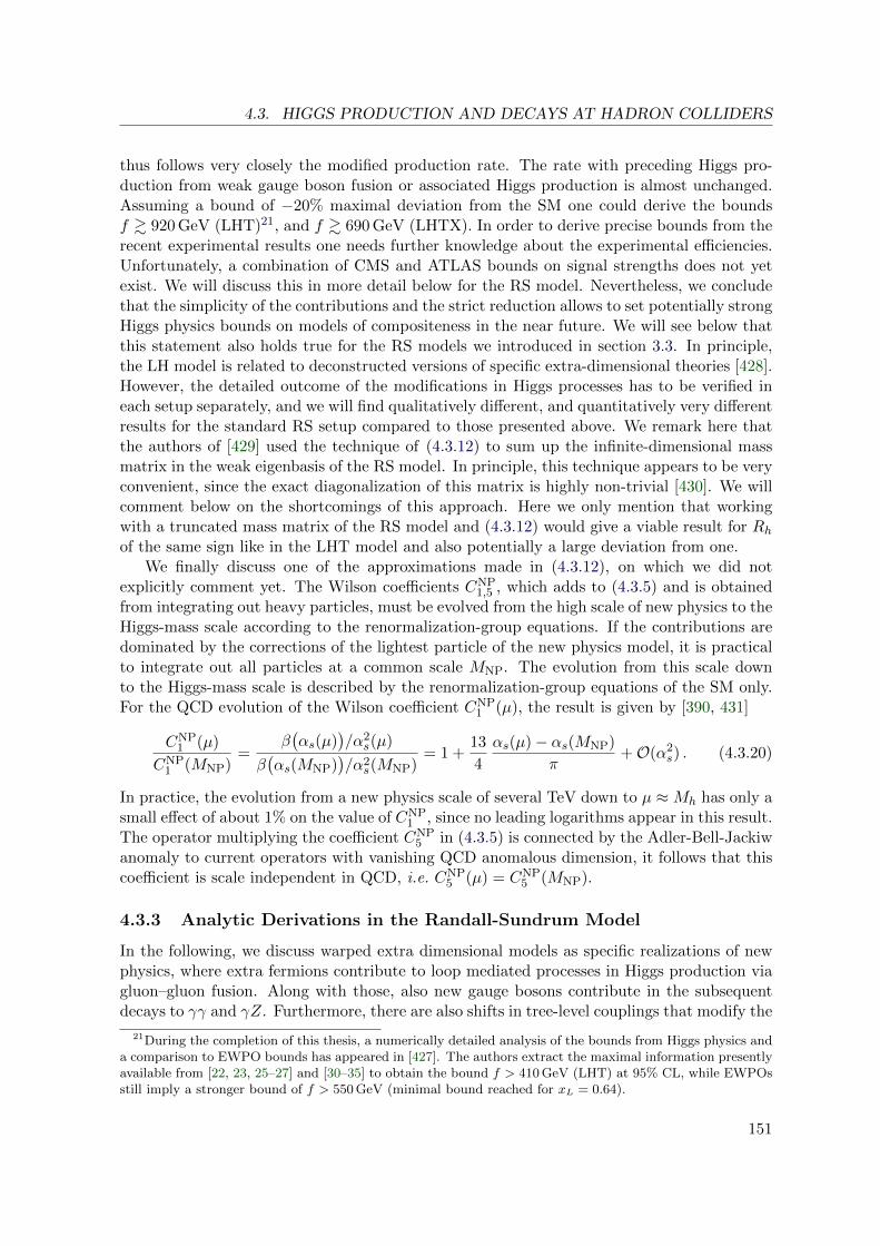
4.3. HIGGS PRODUCTION AND DECAYS AT HADRON COLLIDERS
thus follows very closely the modified production rate. The rate with preceding Higgs pro-duction from weak gauge boson fusion or associated Higgs production is almost unchanged.Assuming a bound of −20% maximal deviation from the SM one could derive the boundsf & 920 GeV (LHT)21, and f & 690 GeV (LHTX). In order to derive precise bounds from therecent experimental results one needs further knowledge about the experimental efficiencies.Unfortunately, a combination of CMS and ATLAS bounds on signal strengths does not yetexist. We will discuss this in more detail below for the RS model. Nevertheless, we concludethat the simplicity of the contributions and the strict reduction allows to set potentially strongHiggs physics bounds on models of compositeness in the near future. We will see below thatthis statement also holds true for the RS models we introduced in section 3.3. In principle,the LH model is related to deconstructed versions of specific extra-dimensional theories [428].However, the detailed outcome of the modifications in Higgs processes has to be verified ineach setup separately, and we will find qualitatively different, and quantitatively very differentresults for the standard RS setup compared to those presented above. We remark here thatthe authors of [429] used the technique of (4.3.12) to sum up the infinite-dimensional massmatrix in the weak eigenbasis of the RS model. In principle, this technique appears to be veryconvenient, since the exact diagonalization of this matrix is highly non-trivial [430]. We willcomment below on the shortcomings of this approach. Here we only mention that workingwith a truncated mass matrix of the RS model and (4.3.12) would give a viable result for Rhof the same sign like in the LHT model and also potentially a large deviation from one.
We finally discuss one of the approximations made in (4.3.12), on which we did notexplicitly comment yet. The Wilson coefficients CNP
1,5 , which adds to (4.3.5) and is obtainedfrom integrating out heavy particles, must be evolved from the high scale of new physics to theHiggs-mass scale according to the renormalization-group equations. If the contributions aredominated by the corrections of the lightest particle of the new physics model, it is practicalto integrate out all particles at a common scale MNP. The evolution from this scale downto the Higgs-mass scale is described by the renormalization-group equations of the SM only.For the QCD evolution of the Wilson coefficient CNP
1 (µ), the result is given by [390, 431]
CNP1 (µ)
CNP1 (MNP)
=β(αs(µ)
)/α2
s(µ)
β(αs(MNP)
)/α2
s(MNP)= 1 +
13
4
αs(µ)− αs(MNP)
π+O(α2
s) . (4.3.20)
In practice, the evolution from a new physics scale of several TeV down to µ ≈Mh has only asmall effect of about 1% on the value of CNP
1 , since no leading logarithms appear in this result.The operator multiplying the coefficient CNP
5 in (4.3.5) is connected by the Adler-Bell-Jackiwanomaly to current operators with vanishing QCD anomalous dimension, it follows that thiscoefficient is scale independent in QCD, i.e. CNP
5 (µ) = CNP5 (MNP).
4.3.3 Analytic Derivations in the Randall-Sundrum Model
In the following, we discuss warped extra dimensional models as specific realizations of newphysics, where extra fermions contribute to loop mediated processes in Higgs production viagluon–gluon fusion. Along with those, also new gauge bosons contribute in the subsequentdecays to γγ and γZ. Furthermore, there are also shifts in tree-level couplings that modify the
21During the completion of this thesis, a numerically detailed analysis of the bounds from Higgs physics anda comparison to EWPO bounds has appeared in [427]. The authors extract the maximal information presentlyavailable from [22, 23, 25–27] and [30–35] to obtain the bound f > 410 GeV (LHT) at 95% CL, while EWPOsstill imply a stronger bound of f > 550 GeV (minimal bound reached for xL = 0.64).
151
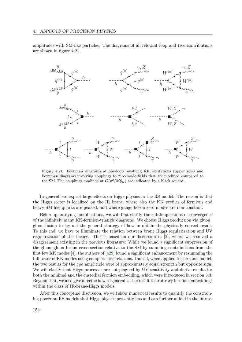
4. ASPECTS OF PRECISION PHYSICS
amplitudes with SM-like particles. The diagrams of all relevant loop and tree contributionsare shown in figure 4.21.
g
g
hq(n)
q(n)
q(n)h
!, Z
!
q(n)
q(n)
q(n)
h
!, Z
!
W (n)
W (n)
W (n)
!!
O
g
g
ht
t
t
!h
b, t
b, t
!h
W, Z
W, Z
!
h
!
!
t
t
t!h
!
!
W
W
W!h
Z
!
t
t
t!
!
h
Z
!
W
W
W!
$ ' $ & '.
Figure 4.21: Feynman diagrams at one-loop involving KK excitations (upper row) andFeynman diagrams involving couplings to zero-mode fields that are modified compared tothe SM. The couplings modified at O(v2/M2
KK) are indicated by a black square.
In general, we expect large effects on Higgs physics in the RS model. The reason is thatthe Higgs sector is localized on the IR brane, where also the KK profiles of fermions andheavy SM-like quarks are peaked, and where gauge boson zero modes are non-constant.
Before quantifying modifications, we will first clarify the subtle questions of convergenceof the infinitely many KK-fermion-triangle diagrams. We choose Higgs production via gluon–gluon fusion to lay out the general strategy of how to obtain the physically correct result.To this end, we have to illuminate the relation between brane Higgs regularization and UVregularization of the theory. This is based on our discussion in [2], where we resolved adisagreement existing in the previous literature: While we found a significant suppression ofthe gluon–gluon fusion cross section relative to the SM by summing contributions from thefirst few KK modes [4], the authors of [429] found a significant enhancement by resumming thefull tower of KK modes using completeness relations. Indeed, when applied to the same model,the two results for the ggh amplitude were of approximately equal strength but opposite sign.We will clarify that Higgs processes are not plagued by UV sensitivity and derive results forboth the minimal and the custodial fermion embedding, which were introduced in section 3.3.Beyond that, we also give a recipe how to generalize the result to arbitrary fermion embeddingswithin the class of IR-brane-Higgs models.
After this conceptual discussion, we will show numerical results to quantify the constrain-ing power on RS models that Higgs physics presently has and can further unfold in the future.
152

4.3. HIGGS PRODUCTION AND DECAYS AT HADRON COLLIDERS
4.3.3.1 General Strategy for Loop Mediated Processes
The general form of the effective low-energy Lagrangian for ggh couplings was given in (4.3.5).In the following, we integrate out all KK quarks at the energy scale MKK. The correspondingtriangle diagram is depicted in figure 4.22 and the LO results are analogous to the top- andbottom-quark contribution of the SM discussed in section 4.3.1. Finally we also parametrizethe shifts in the top- and bottom-quark contribution.
q(n)
q(n)
q(n)
g
g
h
Figure 4.22: Virtual KK-quark contribution to the effective ggh couplings.
The unbroken SU(3)c implies gluon couplings to fermions that are diagonal in the massbasis. Thus, in any case a single KK-quark state q(n) runs in the loop. We gave the relevantcouplings in (3.3.130) and (3.3.131). In the following, we abbreviate gqnn ≡ gRhqnqn and needthe diagonal couplings only
Ldiaghqq = −
∑
q=u,d
∑
n
[Re(gqnn)h q(n)q(n) + Im(gqnn)h q(n) iγ5 q
(n)]. (4.3.21)
The couplings are in general complex numbers, such that pseudo-scalar currents appear inthe Lagrangian. In principle, these could have interesting implications for phenomenology[432]. However, the imaginary parts of the Yukawa couplings for SM-like fermions are verystrongly suppressed in the RS model, as we have shown in section 3.3.8.1.
At the matching scale µ = MKK, the Wilson coefficients entering (4.3.5) have the simpleone-loop results
CKK1 (MKK) =
∑
q
∑
n
′ v Re(gqnn)
mqn
Ahq (τqn) ,
CKK5 (MKK) =
∑
q
∑
n
′ v Im(gqnn)
mqn
Bhq (τqn) ,
(4.3.22)
where τqn = 4(mqn)2/m2
h − iε. The prime on the summation symbol indicates that theyextend over all KK-fermion states but exclude the zero modes, i.e. SM fermions n = 1, 2, 3for q = u, d.
Since the KK quarks are much heavier than the Higgs boson, it is sufficient to use theasymptotic values Ahq (∞) = Bh
q (∞) = 1 of the form factors. Even for quark masses as light as1 TeV, the error of this approximation is sub per-mil. This implies that the relevant quantitywe need to compute is given by
CKK1 (MKK) + i CKK
5 (MKK) =∑
q
∑
n
′ vgqnnmqn. (4.3.23)
The real part of the sum (4.3.23) determines CKK1 , while the imaginary part gives CKK
5 .
153

4. ASPECTS OF PRECISION PHYSICS
We recall at this stage that both the Yukawa couplings and the mass eigenvalues depend onthe regulator η used to smear out the Higgs profile. In addition, one needs to worry about theconvergence of the infinite sum over KK modes. Indeed, since the Yukawa couplings gqnn are ofO(1) and the masses of the KK modes are approximately evenly spaced multiples of the KKscale, naively one expects the sum in (4.3.23) to diverge logarithmically. Power counting foran infinite extra dimension would of course also suggest this. Taking into account 4d-gaugeinvariance22, we would have in D infinite space-time dimensions, with Ebos = 3 externalbosons, and mass dimension [gV ] of the vertices V , a superficial degree of divergence
ωD(“triangle”) = D − D−22 Ebos −
∑
V
[gV ]− 2
= D − D−22 × 3− 3× 4−D
2 − 2 = D − 5 .
(4.3.24)
Of course this is not the final answer. The additional momentum integral of an infinite extradimension reduces to an infinite sum over the KK resonances, which have a specific structure.For the given non-trivial background metric, power-counting arguments loose their powerto assess the renormalization structure intuitively. An example of a careful power countingfor the process µ → eγ has been performed in [230], however without taking into accountregularization issues of the brane-Higgs profile. It shows the necessity to account for manypeculiarities of the practical loop calculation. For this reason, we will not dwell on sucharguments, since the additional insight is little, and instead discuss the physics by using theexplicit calculation.
In order to define the sum in (4.3.23) properly, we regularize it by considering the partialsum up to a given highest KK level
Σq(N, η) =
nf+NnF∑
n=1
vgqnnmqn. (4.3.25)
This sum now includes the nf SM-like quarks plus the first N KK levels, where nF is thenumber of KK modes per KK level. The notation is kept general like in section 3.3.118 inorder to apply it to any fermion embedding. It will turn out that the sum over modes isfinite despite naive expectation, because non-trivial cancellations happen among the modescontained in each KK level. Nevertheless, yet another, third regularization is present in thecalculation, associated with the UV behavior of the theory. We discussed the reasons togenerally regulate the 4d fermion-triangle calculation gauge invariantly in section 4.3.1. Wealso discussed in section 3.3.7 that in order to account for the gauge-hierarchy problem inRS, we must limit the range of validity of the model as an EFT. These two aspects becomeimportant in the following.
Concerning Σq(N, η), practically we are left with a choice of the order of limits η → 0 andN → ∞. We will see that the limits do not commute. In most of the literature the Yukawacouplings are evaluated mode by mode, taking the regulator η to zero after computing therelevant overlap integrals. In [4] we took this approach to discuss the Higgs phenomenologyin the custodial RS model. Here, it corresponds to taking the limit η → 0 first, and hence
Σ(low)q ≡ lim
N→∞
[limη→0
Σq(N, η)]
= limN→∞
nf+NnF∑
n=1
[vgqnnmqn
]
η→0
. (4.3.26)
225d gauge invariance is broken by BCs and not spontaneously.
154

4.3. HIGGS PRODUCTION AND DECAYS AT HADRON COLLIDERS
The alternative approach taken e.g. in [429, 433], considers the infinite sum over modes fromthe very beginning. This is accomplished by means of completeness relations for the fermionprofiles. The regularization of the Higgs profile is taken to zero at the end of the calculation,such that this approach corresponds to
Σ(res)q ≡ lim
η→0
[limN→∞
Σq(N, η)
]= lim
η→0
∞∑
n=1
vgqnnmqn. (4.3.27)
In the following sections, we will derive closed analytical expressions for the limiting valuesin both cases – (4.3.26) and (4.3.27) – and subsequently discuss the physical interpretationof the results. For the rest of this section, we denote with Σq any of the two limiting orders.
First we return to the Wilson coefficients in (4.3.23). Using the full sum over all KK levelsΣq we have to subtract the contributions from in KK level N = 0, i.e. the SM quarks, eachof which equals 1 up to higher-order corrections in v/MKK. By writing
limη→0
Σq(0, η) =∑
n=1,2,3
limη→0
vgqnnmqn
= Σ0q − εq , (4.3.28)
we split the result into a bulk mass independent part Σ0q , and dependent part εq. The latter
is given by
εq = Tr[ΦQ + Φq
]+O
(v4
M4KK
)≈(ΦQ
)33
+(Φq
)33. (4.3.29)
In the minimal and custodial RS model of sections 3.3.4.2 and 3.3.5.2, we obtain
•minimal (q = u, d) :
Σ0q = Tr
[2Xq
sinh(2Xq)
]= Tr
[atanh
(Xq
) (X−1q − Xq
)], (4.3.30)
• custodial (q = u, d) :
Σ0q = Tr
[2√
2Xq
sinh(2√
2Xq)
]= Tr
[atanh
(√2Xq
) ((√
2Xq)−1 −
√2Xq
)]. (4.3.31)
For notational convenience we also set Σ0λ ≡ ελ ≡ 0 .
The matrices Xq and Xq were defined in (3.3.41). They depend only on the order onefundamental Yukawa matrices and the ratio v/MKK. For the bulk mass independent part,the difference in going from the minimal to the custodial model is given by the additionalfactor of
√2 in front of Xq. This is easily understood from the multiplicity of the enlarged
fermion sector with twisted BCs. In fact (3.3.41) implies that the misalignment between thefundamental Yukawa matrices Y~q and the ones defining the spectrum Y~q results in
√2Xq =
tanh(√
2Xq) for q = u, d. The bulk mass dependent part εq is a subleading correction in mostof the parameter space. It receives its main contribution from the third-generation terms,since the quantities
(ΦQ,q
)nn
defined in (3.3.132) are chirally suppressed for all light quarks.The Wilson coefficients for the sectors of common charge are finally obtained as
CKKq,1 (MKK) + i CKK
q,5 (MKK) = Σq − Σ0q + εq , CKK
i (MKK) =∑
q=u,d(,λ)
CKKq,i (MKK) . (4.3.32)
155

4. ASPECTS OF PRECISION PHYSICS
Note that, like Σ0q , we will see below that the full sum Σq also turns out to be real. The pseudo-
scalar Wilson coefficient is therefore given by CKK5 (MKK) = Im (εu + εd) and receives only
contributions of O(v4/M4KK), which have been neglected in the expression for εq in (4.3.29).
Nevertheless, we will keep the discussion general in the following and use exact results in thenumerical evaluation of section 4.3.4.
The cross section for Higgs production in gluon–gluon fusion can be written as
Rh =σ(gg → h)RS
σ(gg → h)SM=
∣∣κg∣∣2 +
∣∣κ5g
∣∣2
κ2v
. (4.3.33)
The factors κg and κ5g encode the LO ratio of the non-interfering CP -even and CP -odd RSamplitude, divided by the total SM amplitude
κg =CKK
1 (Mh) +∑
i=t,b Re(κi)Ahq (τi)∑
i=t,b Ahq (τi)
,
κ5g =3
2
CKK5 (Mh) +
∑i=t,b Im(κi)B
hq (τi)∑
i=t,b Ahq (τi)
.
(4.3.34)
Here, the factors κq = vgq33/mq introduce modifications of the Higgs-boson couplings totop and bottom quarks with respect to their SM values. In the SM cross section (4.3.4),the dependence on the Higgs VEV was factored out as (vSM)−2, with the rest of the resultdepending on input masses only. We proceed similarly with the RS result, using the modifiedVEV v of the RS model as calculated in (4.2.19). The factor κv in the denominator of (4.3.33)accounts for this shift. Consequently, κg and κ5g are linear in the VEV v, which has beenused here for κq and (4.3.22), and no further factors of κv are involved in the correspondingexpressions.
In order to obtain a simple formula for κq, we employ (3.3.131) and the ZMA result(3.3.139) and furthermore expand in the Cabibbo angle using a Froggatt-Nielsen expansionas explained in section 3.3.4.2. The result reads
κq ≈ 1− (ΦQ)33 − (Φq)33 −v2
3M2KK
(YqY
†q Yq
)33
(Yq)33
·
1 , minimal RS
2 , custodial RS. (4.3.35)
Remark that the bulk-mass dependence in (4.3.35) is the same that also dominates bulk-massdependent part of the Wilson-coefficient of heavy KK contributions. As shown in (4.3.29),it enters the latter with a negative sign. Consequently, the dominant bulk mass dependentcontributions from the top quark enter the final expression (4.3.34) only proportional to thedifference Ahq (τt)− 1 ≈ 4%, i.e. they cancel to a large extent.
4.3.3.2 Evaluation of the Two Regulator Limits
We are now ready to evaluate the two alternative regulator limits leading to the full sums of(4.3.26) and (4.3.27). We begin with examining the sum in (4.3.27), in which the regulatorof the Higgs profile is removed after the infinite sum over KK modes has been performed.The authors of [429] succeed to evaluate this sum with the completeness relations (3.3.30) forthe fermion profiles. The analysis relies on a perturbative treatment of Yukawa couplings,which yields the first non-trivial contribution in the expansion in v2/M2
KK. A subtlety in
156
4.3. HIGGS PRODUCTION AND DECAYS AT HADRON COLLIDERS
this calculation, worth recalling, is that in the perturbative approach the odd fermion profiles
S(A)n (t) vanish on the IR brane. As a result, the contribution of each individual mode, and
hence of any truncated KK sum, vanishes in the limit where the width of the Higgs-bosonprofile is taken to zero. A non-zero result for the O(v2/M2
KK) correction to (4.3.27) is obtainedonly after summing over the infinite tower of KK states.
An elegant way to derive a closed expression for the sum (4.3.27), valid to all ordersin v/MKK, is to relate it to the 5d fermion propagator of the theory. We proceed similar to[236], where this method has been applied to a model of 5d gauge-Higgs unification. It followsfrom the second relation in (3.3.129) and (3.3.110) that the infinite sum in (4.3.27), for fixed,non-zero η is given by
limN→∞
Σq(N, η) =
1∫
ε
dt δη(t− 1)T qRL(t, t) , (4.3.36)
where
T qRL(t, t′) =v√2
Tr
[(0 YqY †q 0
)∆qRL(t, t′)
]. (4.3.37)
Notice that only the off-diagonal blocks of the propagator for 1 − η < t, t′ < 1 enter in thisresult. We find for a general fermion embedding
T qRL(t, t′) = Tr
[y~q eq cosh
(X~q
t>∫
t<
ds δη(s− 1)
)−X~q sinh
(X~q
t>∫
t<
ds δη(s− 1)
)], (4.3.38)
where the normalized Yukawa matrix y~q and the matrix eq have been defined in (3.3.122)and (3.3.124).
Obviously, for the special case t = t′, the trace in (4.3.38) is independent of both t and η.Thus the t-integration in (4.3.36) reduces to the normalization of the Higgs profile, which isindependent of its regularized shape and equal to 1. We conclude that the full sum in (4.3.36)is in fact already independent of η. Remarkably, the infinite sum of KK states converges tothe very simple result
Σ(res)q = Tr
[y~q eq
], (4.3.39)
despite the fact that it is superficially divergent. This hints to the existence of intricatecancellations between different contributions to the sum. In the following, we subsequentlyevaluate (4.3.39) for the minimal and custodial case. After that, we discuss the structure ofthe result for a general fermion embedding in terms of an expansion in v/MKK.
• minimal (q = u, d) :
Σ(res)q = Tr
[Xq coth
(Xq
)]= nf +
1
3Tr[X2q
]+O
(v4
M4KK
). (4.3.40)
The first non-trivial term in the Taylor expansion agrees with the result derived in [429].Note that this result is real, and hence it only contributes to the Wilson coefficient CKK
1 .From (4.3.32) and (4.3.28), we now obtain
CKK1 (res)(MKK) =
∑
q=u,d
(Tr[Xq tanh(Xq)
]+ Re(εq)
)
=∑
q=u,d
Tr[X2q + Re(ΦQ + Φq)
]+O
(v4
M4KK
).
(4.3.41)
157

4. ASPECTS OF PRECISION PHYSICS
The contribution to the coefficient CKK1 is positive and hence yields an enhancement of
the ggh amplitude compared to the SM.
• custodial :
Σ(res)d = Tr
[√2Xd coth
(√2Xd
)],
Σ(res)u = Tr
[√2Xu coth
(√2Xu
)]+ Σ
(res)λ ,
Σ(res)λ = Tr
[√2Xd tanh
(√2Xd
)]= 2 Tr
[X2d
]+O
(v4
M4KK
).
(4.3.42)
We observe that the factor√
2 — which encompasses the extension of the left-handeddoublet to a bidoublet for the up sector, and the right-handed singlet to triplet extensionfor the down sector — leads to a doubling of the new physics contribution comparedto the minimal RS result at leading order in v2/M2
KK. Remark that one would obtainthe same result in the case of an extended fermion sector that is SU(2)L × SU(2)Rsymmetric simply by extending both the down and up-type singlets to doublets withadditional fermions of twisted BCs; a setup studied in [429] that is however at odds withprecision measurements of the ZbLbL-coupling. In the custodial setup, which we employ,there exist even more important new contributions from the exotic fermions of charge5/3 and from new up-type quarks contained in the triplets. Both contributions are
equal and given by Σ(res)λ , which involves the triplet Yukawa coupling Yd (see (3.3.69)).
The total contribution proportional to Yd is then approximately six times larger thanthe down-type new physics contribution in the minimal RS model. This shows that theresult massively depends on the choice of the fermion sector. As a general rule of thumb,new fermions with twisted BCs contribute not proportional to their multiplicity, butthe stronger, the higher their multiplet representation is, due to simple combinatorics.The final Wilson coefficient is given by
CKK1 (res)(MKK) = Tr
[√2Xu tanh
(√2Xu
)]
+ 3 Tr[√
2Xd tanh(√
2Xd
)]+ Re(εu + εd)
= Tr[2X2
u + 6X2d + Re(ΦU + Φu + ΦD + Φd)
]+O
(v4
M4KK
).
(4.3.43)
• generic :In order to understand the model dependence of the contributions in the custodial modelwe can also expand the generic result of (3.3.125) in v/MKK. This provides a compact
result for Σ(res)q , which illustrates the various sources of the leading order contributions
in terms of the sub blocks of the generalized Yukawa matrix
Y~q =
(Y (++)q Y (+−)
q
Y (−+)q Y (−−)
q
). (4.3.44)
Here, the two superscripts indicate the UV BCs of the two fermions that enter thecorresponding Yukawa coupling in the notation of (3.3.23). We obtain
Σ(res)q = nf +
v2
2M2KK
1
3
(Tr[Y (++)q Y (++) †
q
]+ Tr
[Y (+−)q Y (+−) †
q
]+ Tr
[Y (−+)q Y (−+) †
q
])
+ Tr
[(Y (−−)q − 2
3Y (−+)q Y (++)−1
q Y (+−)q
)Y (−−) †q
]+O
(v4
M4KK
).
(4.3.45)
158

4.3. HIGGS PRODUCTION AND DECAYS AT HADRON COLLIDERS
The enhanced contribution from Yukawa couplings Y (−−)q between two fermions with
twisted BCs is a generic feature. The relative sign in the last line suggests that itcould be compensated by mixing between all sectors like present in the up-sector of thecustodial model above. However, for a general triplet-bidoublet coupling like in (3.3.68)the relation Y (+±)
q = ±Y (−±)q holds, such that the two contributions in the last line both
add constructively to the total result.
Now, we switch to the alternative order of regulator limits (4.3.26), for which the limitsN → ∞ and η → 0 are taken in the opposite order compared to (4.3.27). In this case onefirst considers a finite sum over KK modes and derives the relevant Yukawa coupling for eachmode by regularizing the Higgs profile, computing the overlap integral in (3.3.129), and thentaking the limit η → 0. The relevant Yukawa couplings in that limit have been given in(3.3.130).
Since the sum in (4.3.26) extends over a finite number of KK levels, it is not possibleto use the elegant method of 5d propagators described in the previous section. In order toobtain a closed expression nonetheless, we adopt the strategy of first finding a solution in thespecial case of one generation and vanishing bulk masses. In this case the bulk EOMs and theeigenvalue equation that determines the masses of the KK modes can be solved analytically.The relevant spectrum and couplings for this toy model are summarized in appendix A.3. Wewill then generalize the result to nf generations and argue that, as in the case (4.3.40), thegeneral solution is independent of the bulk-mass parameters, too.
Equations (A.3.8) and (A.3.9) imply that in the simplified case we have
limη→0
Σq(N, η)∣∣∣toy
=2N∑
n=0
vgqnnmqn
∣∣∣∣η→0
=Xq
cosh(2Xq)
[1
x0+
N∑
k=1
(1
kπ + x0− 1
kπ − x0
)]. (4.3.46)
In the one-generation case, we refer to the zero mode as n = 0, while n ≥ 1 labels the KKmodes. The first term in the bracket on the right-hand side of (4.3.46) arises from the SM-likequark, while the remaining sum is over pairs of KK modes belonging to the kth KK level.Note that, for large k the individual terms in the sum fall off like 1/k only, but each paircombines to a contribution decreasing like 1/k2. Hence, the sum over KK modes is alternatingand convergent, and it is possible to take the limit N → ∞. We obtain for (4.3.26) in thecase of a single fermion generation with vanishing bulk masses
Σ(low)q
∣∣∣toy
=Xq coth(Xq)
cosh(2Xq)= 1− 5
3X2q +O
(v4
M4KK
). (4.3.47)
This result differs from the finite sum in (4.3.46) only by terms of O(1/N), i.e. it showsproper decoupling behavior as it is expected for usual vector-like fermions. We have explicitlyconfirmed that the result (4.3.47) is stable under variations of the bulk masses. The calculationis summarized in appendix A.3. We also checked independence of the bulk masses numericallyto very high precision.
Before we generalize the last result to nf generations, we want to illuminate the discrep-ancy between the results (4.3.40) and (4.3.47). Obviously, the limits η → 0 and N → ∞ in(4.3.26) and (4.3.27) are non-commutative and will lead to a large difference for the effec-tive ggh couplings, as we can easily observe in the expansion in v/MKK. We will illuminatethe physical origin of this difference in the following. This will later guide our search for aselection criterion of the physically correct result.
159

4. ASPECTS OF PRECISION PHYSICS
n + 1
Figure 4.23: The left panel shows the partial sums Σq(N, η) for different values of n = 2Nand η in the toy model with one generation and vanishing bulk-mass parameters. Thecurves refer to η = 10−2 (red), 10−3 (green), 10−4 (blue), and 0 (black). We denote n+1 onthe logarithmic abscissa in order to include the zero mode. The right panel shows Yukawacouplings gqnn of the KK-fermion states in the toy model for η = 10−3. The dark points arethe Yukawa couplings averaged over a single KK level.
In appendix A.3 we derive the explicit forms of the bulk profiles, masses, and Higgscouplings for the toy model with one generation, vanishing bulk masses, and a box shapedHiggs profile with finite η > 0. It turns out that the nature of the solution differs strongly,depending on the relative size of the KK fermion’s mass in comparison with a new scale.More precisely, the solution changes significantly if mq
n ≈ vYq/(√
2η) = Mweak/η. Here weassume, as usual, that Yq = O(1) are anarchic and light fermion masses are generated bythe zero mode localization. Recall that we can choose Yq real and positive in the case of onegeneration. The appearance of the scale Mweak/η, which for very small η lies far above theTeV scale, is of crucial importance to physically interpret the discrepancy.
Here we demonstrate the emergence of the new scale in the toy model numerically. Tothis end, we obtain the masses and Higgs–fermion couplings from the formulas (A.3.4) and(A.3.6). In the left plot in figure 4.23, we show the numerical results for the regulated sumΣq(n/2, η) as a function of the number of included KK states n, for four different values of η,i.e. we do not carry out any of the two limits in question. For the purpose of illustration wetake Xq = 0.5, and depict also the intermediate steps where only one of the KK states of aKK level is added to the sum. We observe that for low values of n the sum receives alternatingcontributions, but quickly converges towards a value close to the result (4.3.47), which equals0.701 in the present case. Yet, for higher n, there follows an intermediate region, roughlygiven by the range 0.1/η < 2n < 10/η, in which the value of the sum changes by an O(1)amount. After this transition region, the sum converges to the value corresponding to theresult (4.3.40), which equals 1.082 for our choice of Xq. In order to understand the origin ofthe three regions — in particular the appearance of the intermediate region, in which the sumgrows by an O(1) amount despite the fact that the corresponding KK masses are extremelyheavy — we show in the right plot of figure 4.23 the values of the Yukawa couplings gqnn in
160

4.3. HIGGS PRODUCTION AND DECAYS AT HADRON COLLIDERS
our toy model for the choice η = 10−3. For low values of n we derive in (A.3.9) that the Higgscouplings for each pair of KK-fermion states in the same KK level are of equal magnitudebut opposite sign. In this case, we have seen in (4.3.46), that the contribution from the kth
KK level isXq
cosh 2Xq
(1
kπ + x0− 1
kπ − x0
)= − Xq
cosh 2Xq
2x0
k2π2 − x20
, (4.3.48)
forming a quadratically convergent instead of the naively expected harmonic series. Thesituation changes drastically in the intermediate region. We show in (A.3.11) that the cou-plings with odd n vanish, and those with even n reach a maximum, coincidentally both atmqn ≈√
2vYq/η = 2Mweak/η for the given choice of parameters. Thus, there exists a range oflogarithmic growth of the sum, over which its contribution can be qualitatively estimated as
N2∑
k=N1
gavg(k)
kπ≈ 〈gavg〉
πlnN2
N1, (4.3.49)
where 〈gavg〉 denotes the mean value of gavg(k) in the interval k ∈ [N1, N2], in which theaverage coupling in each KK level departs from zero. Physically, this intermediate regionarises because, for fixed η, there exists a minimum KK mass mq
n ∼ Mweak/η beyond whichthe KK-profile functions begin to significantly penetrate the box modeling the Higgs-bosonprofile. When this happens, the cancellation of the Yukawa couplings of KK modes within aKK level is no longer operative. Consequently, the generic logarithmic growth arises, whichwe expected from naive dimensional analysis. Only for yet much higher KK levels, whenthe profiles exhibit a large number of oscillations within the box, the couplings decreasesufficiently fast with k, such that the sum converges to the aforementioned upper limitingvalue.
In light of the fact that Σ(res)q contains order one contribution from very heavy modes and
is therefore sensitive to UV physics, it is worthwhile to investigate the general result (4.3.47)
for Σ(low)q , which excludes this collective, UV resonance effect. In the next section, we will
show that any UV regularization will render the following result for Σ(low)q as being physically
correct.Given the similarity of the result (4.3.47) with equation (4.3.40), we can still profit from
the derivation of Σ(res)q . We conjecture that in the case of three generations a general recipe
to obtain Σ(low)q is to extend Σ
(res)q with additional inverse matrices of cosh(2Xq) inside the
trace.
• minimal (q = u, d) :
Σ(low)q = Tr
[Xq coth
(Xq
)
cosh(2Xq
)]
= nf −5
3TrX2
q +O(
v4
M4KK
). (4.3.50)
Like in (4.3.40) the result is real, such that only CKK1 receives a contribution. Combining
(4.3.32), (4.3.28), and (4.3.50), we find
CKK1 (low)(MKK) =
∑
q=u,d
(− Tr
[Xq tanh
(Xq
)
cosh(2Xq
)]
+ Re(εq)
)
=∑
q=u,d
Tr[−X2
q + Re(ΦQ + Φq
)]+O
(v4
M4KK
).
(4.3.51)
161

4. ASPECTS OF PRECISION PHYSICS
This time the contribution to CKK1 is negative and thus yields a suppression of the
gg → h amplitude compared with the SM. Incidentally, the first term in the expansionin powers of X2
q has the opposite sign from the result (4.3.41). For the purpose of the
numerical evaluation we want to express the result also with the Yukawa matrices Yq,which determine the spectrum
CKK1 (low)(MKK) =
∑
q=u,d
(− f(Xq) + Re(εq)
), (4.3.52)
f(x) ≡ x atanh(x)1− x2
1 + x2. (4.3.53)
• custodial :
Σ(low)d = Tr
[√2Xd
coth(√
2Xd
)
cosh(2√
2Xq
)],
Σ(low)u = Tr
[√2Xu
coth(√
2Xu
)
cosh(2√
2Xu
)]
+ Σ(low)λ ,
Σ(low)λ = −Tr
[√2Xd
tanh(√
2Xd
)
cosh(2√
2Xq
)]
= −2 Tr[X2d
]+O
(v4
M4KK
).
(4.3.54)
Observe that also the sector of exotic fermions contributes negatively to CKK1 this time.
We summarize the contributions to the Wilson coefficients in terms of the function fintroduced in (4.3.53)
CKKd,1 (low)(MKK) = Tr
[− f(√
2Xd) + Re(εq)],
CKKu,1 (low)(MKK) = Tr
[− f(√
2Xu)− f(√
2Xd) + Re(εq)],
CKKλ,1 (low)(MKK) = Tr
[− f(√
2Xd)].
(4.3.55)
In total this leads to the very short final result
CKK1 (low)(MKK) = Tr
[− f(√
2Xu)− 3f(√
2Xd) + Re(εu + εd)]
= −2 Tr[X2u
]− 6 Tr
[X2d
]+O
(v4
M4KK
).
(4.3.56)
We compare this again to the alternative SU(2)L×SU(2)R symmetric quark embedding,which only promotes down- and up-type singlets to doublets, and leads to disfavoredcontributions to the ZbLbL coupling. In that case, the contribution proportional to thedown-type-Yukawa matrices in (4.3.56) would not be enhanced by a factor 3. Thus, thealternative embedding would again give approximately twice the result of the minimalnon-custodial embedding.
The formulas given here reproduce the numerical results obtained in [4]. We checked thiswith the large sample of more than 104 valid parameter points for 3 fermion generations,which we generated for the numerical analysis of the minimal and separately also for thecustodial RS model. The numerical data is described in more detail below. We remark here
162

4.3. HIGGS PRODUCTION AND DECAYS AT HADRON COLLIDERS
that for each parameter point, we calculated the zero modes plus the complete set of the first
4 KK levels and extrapolated the remaining contribution to C(low)1,q by assuming equidistant
KK-mass spacing at higher levels. We found that the resulting contributions to all threesectors of common charge agree with the analytic result (4.3.56) within 1 per-mil.
We did not give a formal proof of (4.3.50) and (4.3.54) for more than one generation,which would be interesting beyond the numerical verification. Symmetry arguments help usto constrain at least the form of the answer. The result for the sum (4.3.26), expressed as
a function of the fundamental parameters of the underlying 5d theory is given by Σ(low)q =
Σ(Yq, cQ, cq). The EOMs (3.3.32) and boundary conditions (3.3.35) are valid in an arbitrarybasis, in which the bulk-mass matrices cA are not necessarily diagonal. These relations areinvariant under a set of three global symmetries. The first one is a symmetry under theexchange of SU(2) doublets and singlets along with Yq ↔ Y †q . In addition, there are twosymmetries related to unitary transformations of the Yukawa and bulk-mass matrices. Whencombined with the fact that in the one-generation case the result is found to be independentof the bulk-mass parameters, these symmetries imply that the quadratic term in Xq mustindeed be of the simple form shown in (4.3.50).
4.3.3.3 UV Regulation as a Decision Criterion
We have seen in the last section that KK fermions with masses far above the TeV scale seem-ingly change the result of Higgs production via gluon–gluon fusion by an O(1) amount. If thiswas the final answer, the theory would be plagued by a UV dependence even though the spe-cific loop processes in question give finite results. Consequently, we would loose predictabilityfor the given process. In the following, we clarify that this is fortunately not the case. Werecall the importance of using a consistent UV regularization scheme when evaluating thegluon–gluon fusion amplitude. This is true in the SM, as we explained in section 4.3, andeven more so in its 5d extensions. Here, we will study two different regularization schemes:dimensional regularization and the use of a hard momentum cutoff. While a dimensionalregulator is particularly convenient in that it preserves gauge and Lorentz invariance, thesecond option is also a natural choice in the present case, since the theory presents only aneffective theory below the Planck scale. Incorporating the effects of quantum gravity requiresa UV completion. In section 3.3.7, we have already touched a peculiar feature of warpedextra-dimensional models: Their effective UV cutoff depends on where the theory is probedalong the extra dimension [103], more precisely, where the involved particles are localized.The physical reason is that due to warping the fundamental length and energy scales changealong the extra dimension. More specifically, the effective cutoff scale at the position t in theextra dimension is of the order of the warped Planck scale
ΛUV(t) ∼MPl e−σ(φ) = MPl
ε
t≡ ΛTeV
t. (4.3.57)
To preserve predictivity, the cutoff should be sufficiently high, so that at least a small numberof KK modes have masses below ΛTeV, and hence ΛTeV/MKK = O(10). Otherwise incalculablethreshold corrections of order Mn
KK/ΛnTeV become important and call for a non-perturbative
treatment of the unspecified UV-completing theory. We stress that imposing a UV cutoff iscrucial in order for the RS model to provide a viable solution to the hierarchy problem. Self-energy contributions of fermions to the Higgs boson’s mass are estimated by naive dimension
163

4. ASPECTS OF PRECISION PHYSICS
analysis to be of the order
δm2h ∼
∑
mf(n)<ΛTeV
h
f (n)
h
f (n)
∼∑
mf(n)<ΛTeV
|Yf (n) |232π2
m2f (n)
M2KK
. (4.3.58)
Since the Higgs–fermion couplings enter quadratically in this case, there are no possiblecancellations between different chiralities, like we saw in the ggh-loop diagrams of the lastsection. Consequently, the divergent behavior is even worse than generically expected by newphysics, due to the multiplicity of the KK spectrum with equidistant masses. Consequently,it is a necessity to localize the Higgs sector at least very near to the IR brane (in the vicinityof t = 1) and to choose an effective cutoff ΛUV(t) of the order of only several TeV for valuesof t that are on the Higgs profile’s support.
The question of how to introduce such a cutoff in practical one-loop calculations is far frombeing trivial and no rigorous scheme exists for how to distribute the cutoffs on the variousmomenta at a given vertex [231]23. However, at loop momenta several times larger thanMKK, external momenta can be neglected and hence there remains a single 4d (euclidean)loop momentum p2
E ≡ −p2 on which the cutoff should be imposed. Employing a t-dependentcutoff associated with every vertex of a Feynman diagram can be thought of as modeling theeffect of a form factor, which accounts for the impact of quantum gravity on energy scalesabove the effective Planck scale at that point. In general, the ti coordinates of the verticesare integrated over the entire bulk (ε ≤ ti ≤ 1), and hence the cutoff values vary between theTeV scale and the fundamental Planck scale. It was shown that this prescription allows forgauge-coupling unification in warped extra-dimensional models [103, 434–437]. The situationsimplifies considerably for one-loop diagrams that contain vertices with Higgs bosons, suchas the relevant diagram in figure 4.22. Denoting the coordinate of the two gluons by t1 andt2 and that of the Higgs boson by t3, the fact that t3 ≈ 1 ensures that the momentum cutoffon the 4d loop integral is
pE ≤ min
ΛUV(t1),ΛUV(t2),ΛUV(t3)
= ΛTeV . (4.3.59)
The same mechanism applied to the 5d calculation of the radiative Higgs mass correction(4.3.58) guarantees that the hierarchy problem is solved in RS models.
In order to UV regularize the loop integral, our first ansatz is to use standard dimensionalregularization of the four-momentum integration d 4−2εp, with ε > 0. We then find that thesum in (4.3.25) gets modified to
nf+NnF∑
n=1
vgqnnmqn
(µ2
(mqn)2
)ε, (4.3.60)
where µ ∼ ΛTeV is the regularization scale. For very large masses mqn µ, the dimensional
regulator gives rise to a suppression, which renders the sum over KK modes convergent evenfor arbitrary O(1) Yukawa couplings. The limits N → ∞ and η → 0 can therefore be takenwithout encountering any ambiguities. The contribution from the region of very heavy KKmodes with mq
n ∼ Mweak/η, which we illustrated in figure 4.23, and which previously gaverise to an unsuppressed contribution of the form (4.3.49), now receives an extra suppression
23We enlisted three non-equivalent examples in footnote 17 of section 3.3.7
164

4.3. HIGGS PRODUCTION AND DECAYS AT HADRON COLLIDERS
factor η2ε, and vanishes when one takes the limit η → 0 (at fixed ε). The infinite sum thencoincides with the result (4.3.26) up to harmless O(ε) corrections.
In the dimensional regularization scheme, gauge invariance is manifest in the 4d theory.Since the dimensional regulator also regularizes the infinite KK sum, we are guaranteed thatthe 5d theory remains gauge invariant, too. On the other hand, dimensional regularizationis perhaps not the most intuitive way in which to introduce a UV cutoff. As an alternative,we will therefore rephrase the discussion in a regularization scheme based on using the hardmomentum cutoff given in (4.3.59). In order to ensure 4d gauge invariance in this case, wefirst extract two powers of the external gluon momenta by taking appropriate derivatives,after which the remaining loop integral is superficially convergent. Introducing the UV cutoffon this integral, and neglecting the Higgs mass compared with mq
n, we obtain
nf+NnF∑
n=1
2vgqnn
Λ2TeV∫
0
dp2E p
2E
mqn(
p2E + (mq
n)2)3 =
nf+NnF∑
n=1
vgqnnmqn
(Λ2
TeV
Λ2TeV + (mq
n)2
)2
. (4.3.61)
For small masses mqn ΛTeV this reduces to the simple expression vgqnn/m
qn used in the sum
(4.3.25). For very large masses mqn ΛTeV, on the other hand, the UV cutoff gives rise
to a strong suppression proportional to Λ4TeV/(m
qn)4, implying that such heavy KK modes
decouple rapidly. It follows that, due to physical reasons, the sum over KK modes in (4.3.25)is effectively truncated once the KK masses exceed the scale ΛTeV. In the RS model with aHiggs sector that is sufficiently brane-localized, e.g. for the IR-brane Higgs discussed here,the scale Mweak/η at which the very heavy KK modes start to contribute logarithmicallyto Σq(N, η) is parametrically much larger than the effective cutoff scale ΛTeV. It is thenappropriate to truncate the sum at a value Nmax
KK ∼ ΛTeV/MKK corresponding to KK massesmuch smaller than Mweak/η. It follows that
limη→0
Σq(NmaxKK , η) = Σ(low)
q +O(Nmax
KK v2
Λ2TeV
), (4.3.62)
where the truncation error has the form of a threshold correction, which is always present ineffective-theory calculations. Even in the case that only a single KK level is perturbative, theerror remains below 2%.
We can summarize the above discussion by emphasizing the subtle fact that, in orderto obtain the correct answer for the gluon–gluon fusion cross section in the RS model, it isessential to employ a consistent UV regularization scheme when evaluating the loop integral,despite the fact that the integral is convergent. When this is done, the convergence of thepartial sum in (4.3.25) is improved in such a way that the order in which the two limitsN → ∞ and η → 0 are taken becomes irrelevant. Specifically, in the two regularizationschemes we have considered in our analysis, we find
limN→∞η→0
nf+NnF∑
n=1
vgqnnmqn−→
∞∑
n=1
vgqnnmqn
(µ2
(mqn)2
)ε∣∣∣∣η=0
= Σ(low)q +O(ε) , dim.reg. ,
∞∑
n=1
vgqnnmqn
(Λ2
TeV
Λ2TeV + (mq
n)2
)2∣∣∣∣η=0
= Σ(low)q +O
(Nmax
KK v2
Λ2TeV
), cutoff .
(4.3.63)In both schemes the infinite sums are superficially convergent.
165

4. ASPECTS OF PRECISION PHYSICS
The terms suppressed by a power of the UV cutoff, which appear on the right-hand side
of (4.3.62), parametrize the difference between the asymptotic value Σ(low)q of the infinite sum
and the sum over a finite number of KK modes. More generally, such threshold terms mayalso arise from the yet unknown effects of the UV completion of the RS model. From a low-energy perspective, the only requirement on such a completion that is relevant to us is thatit must cure the hierarchy problem by taming loop momenta that exceed the fundamentalscale of quantum gravity. As long as this is the case, the gluon–gluon fusion amplitude willalso be regularized in the way discussed above. In the context of a specific UV completion,the threshold effects could be modeled at low energies by means of a brane-localized effectivehGaµν G
µν,a operator, suppressed by v/Λ2TeV. The additional factor Nmax
KK reflects the highmultiplicity of degrees of freedom in the low-energy EFT. For quite generic reasons, thecoefficient of this operator must contain the loop factor αs(µ)/(4π) factored out in (4.3.5),even in cases where the UV completion of the RS model is strongly coupled. The reason isthat the on-shell external gluons couple proportional to their QCD charges, and that any newheavy state that couples to the Higgs boson must be color neutral, so it cannot have a tree-level coupling to gluons. Hence, a generic UV completion will indeed give rise to a threshold
correction of the form shown in (4.3.62). However, the difference between the two sums Σ(low)q
(4.3.26) and Σ(res)q (4.3.27) cannot be attributed to such a brane-localized threshold term. As
we have shown, it is instead determined by the absence or presence of a physical UV regulatorand a sensible UV completion.
4.3.4 Phenomenology of the Randall-Sundrum Model
In the following, we shall quantify the implications of the RS model for the main channelsof Higgs production and decays at Hadron colliders. To this end, we study the expecteddeviations from the SM amplitudes. They are already constrained by the experimental resultson signal strengths as discussed in section 4.3.1. Again, we use a fixed reference mass ofMh = 126 GeV for the Higgs boson.
4.3.4.1 Production Channels
In the last section, we already laid out the relevant results to study the most important Higgsboson production channel via gluon–gluon fusion. We gave the relevant formula for the shiftin the production cross section Rh in (4.3.33). For the Wilson coefficient CKK
1 , we use andverify numerically the analytic result (4.3.52), which we have shown to be physically viable,and for which the RS contributions decouple with the scale of new physics MKK. We neglectthe sub-percent threshold effects appearing in (4.3.62). This is to be understood implicitlyfor the remaining discussion.
We observed two important aspects for the dominant CP -even part of the RS amplitudeparametrized by κg relative to the SM amplitude. First of all, we have seen that the de-pendence on fermion-bulk masses cancels to a large extent. Neglecting b-quark corrections,setting the top-form factor to one (approximately 5%, and 3% error respectively), using theapproximation (4.3.29), and the Froggatt-Nielsen approximation (4.3.35) (both less than 1%error), we obtain
κg ≈ 1− v2
3M2KK
(YqY
†q Yq
)33
(Yq)33
12
− Tr
[f(Xu) + f(Xd)
f(√
2Xu) + 3f(√
2Xd)
], (4.3.64)
166

4.3. HIGGS PRODUCTION AND DECAYS AT HADRON COLLIDERS
where the upper and lower constants in the curly brackets hold for the minimal and thecustodial RS model. In the following, we will always use the full expression for derivingnumerical results, while making as few approximations as possible. The general behavior andthe suppression of κg can however be well understood from (4.3.64). The second importantinsight was that all KK-fermion-triangle contributions can be expressed by the trace of theanalytic function f(Xq) defined in (4.3.53), with Xq defined in (3.3.41). This is also truefor KK-fermion contributions to the decay into two gluons and two photons. The trace isdetermined by the non-negative, real square roots yiq of the eigenvalues of the hermitian
matrices Yq Y†q as
Tr f(Xq) =∑
i
f
(v yiq√2MKK
), where U Yq Y
†q U† = diag(yiq)
2 . (4.3.65)
An additional factor√
2 enters the arguments in the custodial model. Since the RS modelis able to explain flavor hierarchies by localization in 5d, it is a feature of the model thatthe fundamental Yukawa matrices are structureless and of order one. Thus, the above resultis roughly proportional to the rank of the Yukawa matrices, which is equal to the numberof fermion generations. In other words, the KK towers of all six quarks in the minimal RSmodel give comparable contributions to the effective ggh vertex, irrespective of the massof the corresponding SM fermion. In the custodial model, the sectors of different fermioncharges get the relative weight factors included in (4.3.64), which are constant integers andstill independent of the SM-fermion masses. This property is different from several otherextra-dimensional extensions of the SM. For instance, in models based on universal extradimensions, the 5d Yukawa couplings are hierarchical like in the SM, and hence the Higgsboson couplings to light fermions and their KK excitations are strongly suppressed [438].Models of gauge–Higgs unification have the peculiar property that their contribution fromKK excitations cancels the dominant effect from corrections to the Yukawa couplings of theSM quarks in the ggh amplitude. This leaves only chirally suppressed corrections, which arevery small for all quarks except the top quark [236]. Hence, in these new-physics scenariosonly the top quark and its heavy partners contribute to the effective ggh couplings, whileHiggs boson production is independent of the masses and couplings of the KK excitationsof light SM quarks. In this sense, such models are similar to four-dimensional models wherethe Higgs boson is realized as a pseudo-Nambu-Goldstone boson. We discussed examples insection 4.3.2.
We generated large sets of valid parameter points for the two RS variants discussed here.We have seen above that a strong dependence on the general size of the fundamental Yukawaelements is to be expected. Thus we generated parameters sets for multiple discrete valuesof ymax, where the elements of the Yukawa matrices are constrained by the condition ymax >(Yq)ij > ymax/10 and follow a uniform random distribution in this range. The lower boundsare irrelevant in practice, but included here for definiteness. Further details on the parametersets, as well as intermediate results for the various values of ymax are included in appendix B.4.
As a first check of the data sets and the results entering (4.3.65), we fit a polynomial ofsecond order to the median of the distribution for κt + εu in dependence on the scale MKK.We expect from (4.3.35) roughly a quadratic scaling with ymax. Indeed, we find that theparametrization 1 + c v2 y2
max/(2M2KK) reproduces the behavior very well for MKK > 1.5 TeV
and for all relevant values of ymax. In the minimal and custodial model the coefficient c isof the expected size, 1.15 and 2.10 respectively, as obtained from a fit for ymax = 3. The
167

4. ASPECTS OF PRECISION PHYSICS
deviation from the quadratic scaling can be significant for low values of MKK. The fourthorder term induces a relative contribution of approximately +10% for MKK = 1 TeV, whenincluded in the fit. The Higgs–top coupling is thus somewhat less suppressed than naivelyexpected for large values of ymax/MKK. Deviations from quadratic scaling are even morepronounced for the resummed KK-tower contribution. To see this, we also fit the medians off(Xu,d) with the fit-model function
med(f(Xq)
)= 3
(1− b v2
2M2KK
)f(a x) , (4.3.66)
where x = v ymax/(√
2MKK) in the minimal, and x = v ymax/MKK in the custodial model.Again, this reproduces the numerical results well for MKK > 1.5 TeV. Leaving a and b in(4.3.66) as a free fit parameter, we obtain for the custodial and minimal model, values ofymax = 0.5 . . . 3, and for q = u, d, indeed in every possible combination a value betweena = 0.97–1.03. However, the higher order correction b becomes quite important for low valuesof MKK. For instance, for the custodial model, MKK = 1.5 TeV, and ymax = 3, we get arelative correction of approximately -30% from the non-vanishing value of the coefficient b.The parametrization (4.3.66) even fails completely for values of MKK below 1.5 TeV. Thefunction f(x) in fact saturates as x grows and has a maximum at x ≈ 0.7. This behaviordistorts the naively expected parametrization in a very significant way. In the following, werather calculate all cross sections and branching ratios separately for each parameter point,using the full expressions and derive typical values only for the final distribution. This has theadditional advantage that we can access the deviations from the typical values, i.e. quantifythe spread due to the new physics input parameters.
Figure 4.24: Fitted modification factor of the Higgs production rate via gluon–gluon fusionin the RS model with ymax = 3 compared to the SM. The left plot shows the minimal RSmodel, while the right plot shows the custodially protected model. The cyan lines are the5%, 20%, 50%, 80%, and 95% quantiles. The points of the numerical scan are underlaid infaint yellow and only visible in regions where many points cluster, in order to qualitativelycheck the inclusiveness of the bands.
We show in figure 4.24 the distributions obtained for Rh in the minimal and custodial
168

4.3. HIGGS PRODUCTION AND DECAYS AT HADRON COLLIDERS
model in the left and right panel for the most natural range, which is restricted by ymax = 3.The maximal value corresponds to the perturbativity bound derived in [211] by means ofnaive dimensional analysis. The plots show the median value and the two-sided 60%, and 90%quantile of the parameter distribution, after imposing constraints on viable fermion massesand mixing angles, as a function of the scale MKK. Recall that often also the lightest KK gluonmass MG(1) ≈ 2.45MKK is used as a reference, as its value is a model-independent predictionfor all RS scenarios with common warp factor ε. We observe a suppression of Higgs productionvia gluon–gluon fusion that is large and decouples slowly with MKK. It is predominantlydue the large contribution from KK loops, which can even completely compensate the SMamplitude for very low values of MKK. This is possible in a broad region around 1.3 TeVin the minimal model. Since the multiplicity of KK states is higher in the custodial model,full compensation of the amplitude is already reached in a region around 2.5 TeV. For evenlower values of MKK the RS contribution can overcompensate the SM amplitude by morethan twice its amount, leading to an effective enhancement of Rh for 5% of the parameterspace below MKK = 1.5 TeV and 20% below MKK = 1.2 TeV. Remark that in order tocalculate these numbers reliably, we had to use the exact expressions for the Higgs–fermioncouplings and the resummed expression for the KK-loop contributions, since v ymax/MKK ≈0.5 (ymax/3) (1.5 TeV/MKK) is not a suitable expansion parameter anymore. A perturbativeansatz with mass insertions up to order v2 would effectively lead to f(x) ≈ x2 and massivelyoverestimate the KK-loop contributions in the low MKK region.
We shortly comment on the quality of the approximation (4.3.64) for Rh, which allowsto easily understand the main contributions of the modified top coupling and includes theanalytic result for the KK loops. We applied the fits in the same way as we did for the exactexpressions used for figure 4.24. As expected, the result agrees well, having a deviation atMKK = 1.5 TeV of 1% in the minimal, and 3% in the custodial model for the largest quantileand even much less deviation for the median. This provides an explicit numerical check forthe analytic results of the Wilson-coefficients from KK-loops (4.3.52) and (4.3.56), since wecalculate the exact distribution of Rh by an explicit summation of the loop contributions ofa few KK levels, and extrapolate the resummed result (see appendix B.4).
We also reconstruct the exact behavior for lower values of ymax (see appendix B.4). Wereduce ymax down to 0.5, where the mean entry of a random Yukawa element is 0.1, i.e. oneorder of magnitude below the natural size. In the left panels of figure 4.25, we show theresulting two-dimensional dependence of the median. The right panels quantify the spreadof the parameter distribution by illustrating the distance of the two-sided 90% quantile fromthe SM result. Supposing a constraint on Rh of maximally 50% deviation, a SM-like centralvalue, and ymax = 3, we could read off a constraint of MKK > 2 TeV in the minimal andMKK /∈ [1.8, 4] TeV in the custodial model. For ymax = 1.5 the numbers would change toMKK > 1.1 TeV and MKK > 2 TeV. However, inferring such a constraint will be challenging,even after the full LHC program. This is due to the large theoretical uncertainty affecting thecross section normalization and the inability to access the partial decay width into gluons24.In [376], a strategy to consider ratios of processes from gluon and vector boson fusion withthe same final Higgs decay was proposed as an intermediate step. The normalization ofgg → h→ V V to the analogous process from weak gauge boson fusion appears interesting, buthas limited prospect, if the cuts applied for selecting weak gauge boson fusion are permeable toa significant amount of gg → h+ 2j events (approximately 30% [376]). The main importance
24Rh is also equal to the partial decay width into gluons relative to the SM Γ(h→ gg)RS/Γ(h→ gg)|SM.
169

4. ASPECTS OF PRECISION PHYSICS
- 0.85
- 0.7
- 0.5 - 0.3 - 0.2 - 0.1
- 0.05- 0.02
1 2 3 4 5 6
0.5
1.0
1.5
2.0
2.5
3.0
MKK @TeV D
y max
medH Rh L -1
- 0.7
- 0.5
- 0.3
- 0.2 - 0.1
- 0.05
- 0.02
1 2 3 4 5 60.5
1.0
1.5
2.0
2.5
3.0
MKK @TeV Dy m
ax
distCL90H Rh ,1L
- 0.85
- 0.85
- 0.7- 0.7 - 0.5
- 0.3
- 0.2
- 0.1
- 0.05
1 2 3 4 5 6
0.5
1.0
1.5
2.0
2.5
3.0
MKK @TeV D
y max
medH Rh L -1
- 0.85
- 0.85
- 0.7
- 0.7 - 0.5- 0.5
- 0.3
- 0.2
- 0.1
- 0.1- 0.05
1 2 3 4 5 60.5
1.0
1.5
2.0
2.5
3.0
MKK @TeV D
y max
distCL90H Rh ,1L
Figure 4.25: Enhancement of the Higgs production rate via gluon–gluon fusion in the RSmodel compared to the SM. The upper row (green shading) shows the results for the minimalmodel and the lower (red shading) for the custodially protected model. In the left panels weshow the distance of the typical, i.e. median, value from the SM result. In the right panelswe give the distance of the 90% two sided quantile of the RS parameter distribution fromthe SM result. The distance is defined to be negative if the quantile band is below one andto be zero if the band overlaps with one.
of the result given here is the general insight that KK-loops can lead to drastic changesin the overall production rate, and that this feature is in many cases not compensated byenhancements of the successive Higgs decays, as we will see below.
In order to better understand the parametric behavior of figure 4.25, we derive a roughtwo-parametric estimate for the median value in the region where v ymax/MKK is a suitable
170

4.3. HIGGS PRODUCTION AND DECAYS AT HADRON COLLIDERS
expansion parameter. We obtain
minimal RS:
Rh ≈ 1− v2
2M2KK
(14.3 y2
max + 3.6)
+v4
4M4KK
(62.6 y4
max + 47.1 y2max + 4.4
),
custodial RS: (4.3.67)
Rh ≈ 1− v2
2M2KK
(51.8 y2
max + 7.3)
+v4
4M4KK
(555.1 y4
max + 930.7 y2max − 109.4
).
The relative error of this parametrization compared to the exact median result is below10% for MKK > 0.55 ymax in the minimal, and MKK > 1.42 ymax in the custodial model.The constant term in parenthesis of the second order coefficient is due to the shifted HiggsVEV κv. The second order ymax dependent coefficient and the fourth order coefficients areestimated from the exact numerical data. We see that the fourth order coefficients are largeand partly counteract the large suppression of the second order coefficients. Nevertheless, thesensitivity of Rh to the overall size of the 5d Yukawa couplings is even more pronounced thanthe one arising from dipole-operator transitions such as B → Xsγ [255]. While the lattercontributions also scale with y2
max, unlike Rh, they are (at the one-loop level) insensitiveto the multiplicity of states in the KK-fermion sector. The main difference is that overlapintegrals with profiles of the light external fermions are involved. This feature underscoresthat precision measurements of the Higgs boson properties provide an extraordinary tool forilluminating the quantum structure of electroweak interactions in RS scenarios.
Particularly, in the minimal RS model, the constraints from EWPOs related to the Zbbcoupling restrict the size of the O(1) Yukawa couplings from below, as shown in figure 4.16.Oblique corrections to EWPOs constrain the KK excitations of SM particles to have massesin the 10 TeV range, i.e. MKK & 4 TeV, what puts them outside of the reach for directproduction at the LHC. Figure 4.25 shows that even for such a high KK-scale there can besignificant virtual effects of KK particles in the Higgs-production cross section, provided thatthe 5d Yukawa couplings are not too small. We also discussed that the bounds from obliquecorrection can be relaxed either by one-loop contributions or by modifications of the model.An example is the LRS model, in which the size L of the extra dimension is reduced [192].For Rh, this would only affect the subleading constant term in (4.3.67) and induce a shift of+4% at MKK = 1.5 TeV.
Suppression effects in gg → h were also reported in [207, 236, 439]. A direct numericalcomparison with our findings is however not possible, since [207] only included zero-modecorrections, while [236, 439] studied RS variants that differ from the specific set-up consideredhere. In [440] the authors studied corrections to gluon–gluon fusion arising from virtualexchange of one light fermionic KK mode without considering the large multiplicity of KKfermions, which we found to be important. There, it is claimed that for a heavy bottom-quarkpartner with a mass mb′ of a few hundred GeV, the Higgs-production cross section via gg → hcan be significantly enhanced. We would like to point out that in order to achieve mb′ MKK
with the embedding of quarks as chosen in section 3.3.5.2, the PLR symmetry has to be brokenstrongly via the bulk-mass parameters of the T1 multiplets by choosing cT1i rather far awayfrom cT2i . First of all, such choices of parameters need to be fine-tuned to reproduce themeasured mass spectrum of the SM quarks for anarchic Yukawa couplings. Secondly, wefound that, the bulk mass dependent terms of the top coupling modification cancel to a large
171

4. ASPECTS OF PRECISION PHYSICS
extent against the bulk mass dependent terms of the resummed KK-loop contribution. Thisresult depends only on the approximation of a unit form factor for all KK quarks, whichis applicable even for the light KK-quark masses considered in [440]. We furthermore addthat choices of cT1i corresponding to a strong breaking of the PLR symmetry lead, barring anaccidental cancellation, to a sizable negative shift in the ZbLbL coupling, which is problematicin view of the stringent constraints arising from the Z → bb pseudo observables discussed insection 4.2.2. As discussed in the previous section, also the authors of [429] attempt to resumall KK-loop contributions. However, their result for the Wilson coefficient is of approximatelyopposite sign, since they take into account the unphysical contribution from infinitely heavyKK resonances, which we have shown to be absent in a properly UV-regulated theory.
1 2 3 4 5 60.2
0.4
0.6
0.8
1.0
MKK @TeV D
Rtr
ee
RVBF, minimalRVBF, custodialRtth , minimalRtth , custodial
Figure 4.26: Ratios for the subleading Higgs production cross sections in RS over the SMresult. The dashed lines show the result in the minimal, while the dotted lines correspondto the custodial RS model. The ratio for the vector-boson-fusion mode also applies toassociated production with a W boson. For the associated production with top quarks, theresult for the median value and the two-sided 90% quantile band are shown for ymax = 3.
Compared to gluon–gluon fusion, Higgs boson production through weak gauge-boson fu-sion, qq(′) → qq(′)V ∗V ∗ → qq(′)h with V = W,Z, receives moderate corrections of around−8% in the minimal and −16% in the custodial model for MKK = 2 TeV, due to a fast decou-pling behavior. However, the corrections become very relevant for a lower KK-scale, namely−14% and −29% or MKK = 1.5TeV. The same reduction also affects associated W -bosonproduction25, qq′ →W ∗ →Wh. We calculate the modification factors of the cross section inRS compared to the SM RVBF = RWh = κ2
v |κW |2 by the ratio of the leading tree-level results.Remark that the shifted Higgs VEV slightly reduces this modification. We show the generalresult in figure 4.26. There, we also show the modification of the cross section of associatedtop-quark-pair production, qq → tt∗ → tth, which experiences a reduction, as well. It is givenby Rtth = Re(κt)
2/κ2v. For values of the KK scale in the ballpark of 2 TeV, this suppression
typically amounts to −20% and −40%.
25The modifications of Z- and W -boson fusion are in principle different in the minimal model, but the totalweak gauge boson fusion rate is dominated by the W due to its larger coupling to quarks.
172

4.3. HIGGS PRODUCTION AND DECAYS AT HADRON COLLIDERS
4.3.4.2 Decays Channels: General Aspects, ZZ, bb
In the following, we quantitatively discuss the modifications of all decay channels that arerelevant and can be observed at the LHC. We have already seen that all production channelsand the tree-level couplings for decays into weak gauge bosons and b-quark pairs are sup-pressed in most of the parameter space. We will show that the most important decay channelinto γγ is on the contrary enhanced. We will investigate the interesting interplay betweenthe modifications in production and decay. Finally, we will discuss the decay into the γZfinal state, which could in principle become phenomenologically interesting in the future, butturns out to be less useful for constraining the RS model.
We start with a general overview of how our intermediate quantities for the Higgs VEVshift and coupling modifications have to be combined in order to form modification ratios forthe partial decay widths
Γ(h→ V V )RS
Γ(h→ V V )SM= κ2
v |κV |2 , V = WW, ZZ ,
Γ(h→ A)RS
Γ(h→ A)SM=|κA|2κ2v
, A = γγ, γZ ,
Γ(h→ ff)RS
Γ(h→ ff)SM=
Re(κf )2
κ2v
, f = b, t ,
(4.3.68)
and the total width of the Higgs
RΓ ≡Γ(h)RS
Γ(h)SM= 1 +
∑
f=bb,WW,ZZ
BR(h→ f)
(Γ(h→ f)RS
Γ(h→ f)SM− 1
)+ BR(h→ gg) (Rh − 1) ,
(4.3.69)where we neglect the modification of branching ratios smaller than BR(h → ZZ) and themodification of BR(h→ τ+τ−). Due to the UV localization of leptons, the latter is expectedto be changed much less than the decay into bb, which we discuss below. Finally, we also con-sider the combined process of production and decay for the restricted case of pure productionfrom gluon–gluon fusion.
Rf ≡[σ(gg → h)BR(h→ f)
]RS[
σ(gg → h)BR(h→ f)]SM
=RhRΓ
Γ(h→ f)RS
Γ(h→ f)SM. (4.3.70)
We consider this quantity to be a guideline for the decays into the ZZ and γγ final state atthe LHC. For a more precise analysis one should sum all production cross sections
εfggF σ(gg → h) + εVBF σ(qq(′) → qq(′)V ∗V ∗ → qq(′)h) + εVh σ(qq′ →W ∗ →Wh) , (4.3.71)
with appropriate weight factors εfX accounting for experimental efficiencies and cuts. Thenecessary data for such an analysis is not publicly available at present. A first step was madeby the experimental collaborations, to break the data into two production categories, oneincluding production from weak gauge boson fusion and the other associated W/Z productiononly [24, 36], but the resulting errors on the signal strengths are in most cases roughly±100%. Meanwhile, for all channels where gluon–gluon fusion dominates, we get a firstestimate of potential constraints from Rf . Moreover, it has been discussed in [376] that agood intermediate solution is to consider ratios Rf/R
′f for different final states f, f ′. If both
173

4. ASPECTS OF PRECISION PHYSICS
final states have similar efficiencies, a large part of the uncertainties from the productionprocesses and also from the total width drops out. The result with our simple definition ofRf is the same. For f = bb, our definition of Rf is of little interest, since the observation ofthis state has to proceed almost exclusively from associated production with a W boson, inorder to suppress the large background.
We begin the numerical discussion with the two largest branching ratios into bb and WW ,in order to understand the behavior of the main modifications of the total Higgs width.Equivalently to the WW channel, we consider ZZ here, as it is more important for laterpurposes. Both channels receive the exact same modification in the custodial model and are100% correlated (at tree level) in the minimal model, where the modifications in the WWchannel are suppressed with c2
w compared to the ZZ channel.
The full numerical results for the total width are displayed in figure 4.27, where we alsoaccount for the subleading modifications included in (4.3.69). For natural values of the Yukawa
1.0 1.5 2.0 2.5 3.0 3.5 4.00.2
0.4
0.6
0.8
1.0
MKK @TeV D
RG
ymax = 3
minimalcustodial
1.0 1.5 2.0 2.5 3.0 3.5 4.00.2
0.4
0.6
0.8
1.0
MKK @TeV D
RG
ymax = 0.5
minimalcustodial
Figure 4.27: Modifications of the total Higgs width for a natural value of ymax (left column)and an order of magnitude lower value (right column). The dashed lines show the medianresult in the minimal, while the dotted lines correspond to the custodial RS model. Theshaded regions indicate the two-sided 90% quantile bands corresponding to the median lineof the same color. Detailed views of the single bands are given in figure B.6.
entries, the depletion in RΓ stems mainly from the reduced width into bb. For MKK = 1.5 TeV,it reaches −28% and −41% in the minimal and custodial model, respectively. We observethat part of this reduction in RΓ does not decouple with ymax. This is obvious for theWW contribution, due to the suppressed WWh coupling, but also applies partly for the bbcontribution, which is affected by the modified Higgs VEV. Even in the limit of vanishingYukawa elements (or heavily fine tuned cancellations) a depletion of −7% and −13% remainsin the given example. This has an interesting effect on the branching ratios into the ZZcompared to the bb state, which we present in figure 4.28. For natural values of the Yukawaentries, a large part of the reduction in the partial and total width cancels in all cases.Nevertheless, the reduction in the bb channel is typically larger such that the branchingratio into bb is typically reduced — and quite severely in the custodial model — while thebranching ratio in ZZ is mostly enhanced. The spread due to the new physics parameter
174

4.3. HIGGS PRODUCTION AND DECAYS AT HADRON COLLIDERS
1.0 1.5 2.0 2.5 3.0 3.5 4.0
0.4
0.6
0.8
1.0
1.2
1.4
MKK @TeV D
BR
Hh®
fL RS
BR
Hh®
fL SM
ymax = 3
f = ZZ , minimalf = ZZ , custodialf = bb, minimalf = bb, custodial
1.0 1.5 2.0 2.5 3.0 3.5 4.0
0.4
0.6
0.8
1.0
1.2
1.4
MKK @TeV DB
RHh
®fL R
SB
RHh
®fL S
M
ymax = 0.5
f = ZZ , minimalf = ZZ , custodialf = bb, minimalf = bb, custodial
Figure 4.28: Modifications of the branching ratios for decays into ZZ and bb. The interpre-tation of the displayed curves and bands is analogous to figure B.6. Detailed views of thesingle bands are given in figures B.3 and B.4.
space is of course large in this region such that no definite claims can be made, except thatlarge enhancements in the bb channel are excluded. The behavior is totally reversed in thecase of an order of magnitude lower Yukawa entries, where the modifications are typicallysmaller but less outspread. This is remarkable, since it allows to constrain the RS setup evenin the case of tuned Yukawa matrices.
We illuminate the possible constraint from the gauge structure in figure 4.29, where weshow the combined modification of production and subsequent decay into ZZ. The generaldependence on ymax and MKK follows closely the dependence of Rh, as shown in figure 4.25.For natural values of ymax above one, the suppression is slightly less than in Rh. For values ofymax below one, the modification shrinks visibly slower than in Rh, since the rising total widthand the suppressed ZZh coupling sets in. We assume a bound of at most 52% suppression,i.e. RZZ > 0.48. This value was found in an unfolding of the recent data attempted in [416]at a CL of 95%. We then derive from the 95% quantile of our parameter distribution of thecustodial model a bound of MKK > 1.1 TeV (first KK-gluon mass MG(1) > 2.8 TeV) for thecase that the Yukawa is an order of magnitude lower than expected, i.e. ymax = 0.5. Thebound becomes higher for natural values of the Yukawa entries, but then one cannot excludea region with low KK-scale: we obtain MKK /∈ [2.0, 3.7] TeV (MG(1) /∈ [4.8, 9.1] TeV). In theminimal model, we derive in the same way a bound below 1 TeV for the order of magnitudereduced, and MKK > 1.9 TeV (MG(1) > 4.7 TeV) for natural Yukawa entries.
We add that for the given Higgs mass, also the decay into a bottom and a strange quarkis in principle possible, since the Higgs couplings have non-vanishing off-diagonal entries inthe RS model. We find even for the custodial model, a KK-scale MKK = 1 TeV and ymax = 3,that 95% of the parameter space give a result for the branching ratio below 8 · 10−3, which isway below the observable levels.
175

4. ASPECTS OF PRECISION PHYSICS
- 0.85
- 0.7
- 0.5 - 0.3 - 0.15 - 0.1
- 0.05- 0.02
1 2 3 4 5 6
0.5
1.0
1.5
2.0
2.5
3.0
MKK @TeV D
y max
medH RZZL -1
- 0.7
- 0.5
- 0.3
- 0.15
- 0.1
- 0.05
- 0.02
1 2 3 4 5 60.5
1.0
1.5
2.0
2.5
3.0
MKK @TeV D
y max
distCL90H RZZ ,1L
- 0.85
- 0.85
- 0.7 - 0.7 - 0.5 - 0.3
- 0.15
- 0.1- 0.05
1 2 3 4 5 60.5
1.0
1.5
2.0
2.5
3.0
MKK @TeV D
y max
medH RZZL -1
- 0.85
- 0.85
- 0.7
- 0.7- 0.5
- 0.5 - 0.3- 0.15
- 0.15
- 0.1
- 0.05
1 2 3 4 5 60.5
1.0
1.5
2.0
2.5
3.0
MKK @TeV D
y max
distCL90H RZZ ,1L
Figure 4.29: Modification factors RZZ for Higgs production and subsequent decay into twoZZ bosons. The upper row (green shading) shows the results for the minimal model andthe lower (red shading) for the custodially protected model. In the left panels we show thedistance of the typical, i.e. median, value from the SM result. In the right panels we givethe distance of the two-sided 90% two sided quantile of the RS parameter distribution fromthe SM result. The distance is defined to be negative if the quantile band is below one andto be zero if the band overlaps with one.
176

4.3. HIGGS PRODUCTION AND DECAYS AT HADRON COLLIDERS
4.3.4.3 The Decay into γγ
We come to the most relevant decay channel into γγ. Similar to (4.3.34) we write the ratioof leading order one-loop diagrams of the RS model relative to the SM as
κγ =
κWAhW (τW ) + CKK
W +∑i=t,b
NcQ2i Re(κi)A
hq (τi) +
∑q=u,d(,λ)
NcQ2q C
KKq,1 +Q2
l CKKl,1
AhW (τW ) +∑i=t,b
NcQ2iA
hq (τi)
.
(4.3.72)All Wilson coefficients are understood to be evaluated at the scale Mh. We neglect κγ5 here,since its relative contribution to κγ is expected to be even smaller than κg5 was for Rh,because of the dominant SM W -boson contribution for a light Higgs mass.
The Wilson coefficient CKKl,1 in (4.3.72) encodes effects from KK-leptons. However, we do
not examine the different possibilities to realize the lepton sector, and the ways to generateright-handed neutrino masses [186, 199, 258, 441]. Here, we only assume a minimal realization,i.e. SM-representations in the minimal model and two SU(2)R doublets that replace thesinglets in the custodial model. Since all KK-fermion contributions add constructively, thisis a conservative way to estimate the minimal effect. Under this assumptions the details ofthe precise lepton spectrum can be entirely omitted to a very good approximation with thefollowing trick [442]. We rewrite the KK-fermion contributions to (4.3.72) by reusing the gghWilson coefficient CKK
1 as
∑
q=u,d,λ
NcQ2q C
KKq,1 +Q2
l CKKl,1 =
4Nc
9CKK
1 +7Nc
3CKKλ,1 +
[CKKl,1 −
Nc
3CKKd,1
], (4.3.73)
where CKKλ,1 is only non-zero in the custodial model, but obviously has a large impact in the
custodial model, due to the enhancement with the squared charge. We now use that — byconstruction of the model — the fundamental Yukawa matrices are random matrices withelements of similar magnitude. The last two terms in square brackets therefore tend to canceleach other, especially since (4.3.65) shows that the function f is mostly determined by the
largest eigenvalue of YqY†q . For the scan over the parameter space, which we present below,
a full inclusion of KK-lepton effects would not change average values and only marginallyincrease the spread, which is dominated by the dependence on the total width as we shall see.We can therefore safely neglect the terms in square brackets in (4.3.73). We emphasize that(4.3.73) relates the most important fermion contribution to κγ , which stems from all fermionswith non-exotic charge Qd,u, to the shift in the ggh amplitude κg. This is an interestingcorrelation, which enhances the constraining power of bounds on the γγ signal strength.
For the evaluation of (4.3.72), it is furthermore necessary to take into account all modifi-cations of the triangle diagram with a weak gauge boson. By working in unitary gauge, it isalso sufficient. Firstly, the WWh-coupling is modified by the factor κW , which was defined in(3.3.152). Furthermore, we also have to include KK-W-boson loops. We resum them by usingthe 5d gauge boson propagator for vanishing momentum, which we derived in section 3.3.7.Observe, that in the case of gauge bosons, each term in the KK-sum over the 4d diagramscarries a mass squared in the denominator. Thus, the sum shows absolute convergence andthere arise no subtleties of the kind we encountered for triangle diagrams with very heavyKK-fermions. In the calculation of the Wilson coefficient CKK
W , we can safely use the decou-pling limit for the form factors. Since mW
1 ≈ 2.5MKK Mh, corrections in the relevant mass
177

4. ASPECTS OF PRECISION PHYSICS
ratio τWn ≡ 4(mWn
)2/M2
h of order O(τ−1W (1)) are sub per-mil. Setting ~dW ≡ (cW ,−sW )T , we
obtain for both, the general custodial, and the minimal RS model (cW = 1) the result
CKKW =
2πM2W
c2WM
2KK
∞∑
n=1
~d TW ~χWn (1) ~χWn (1)T ~dW(xWn)2 AhW
(τW (n)
)
=2πM2
W
c2WM
2KK
~d TW[Σ
(1)W (1, 1)−Π
(1)W (1, 1)
]~dW
(− 21
4+O
(τ−1W (1)
))
= −21
8(1− κW )
(1 +O
(τ−1W (1)
)).
(4.3.74)
We observe that the KK-W contribution is related to the modification of the W contribution.All aspects discussed above are conveniently summarized in a simplified expression for κγ :
κγ = 1 +1
|AhW (τW )| − 43A
hq (τt)− 1
3Ahq (τb)
[− (1− κW )
(|AhW (τW )| − 21
8
)
+ (1− κg)4
3
(Ahq (τt) +Ahq (τb)
)−(1− Re(κb)
)Ahq (τb) + 7(−CKK
λ,1 )
].
(4.3.75)
This simplified result neither relies on any specific quark embedding, nor on the requirementof PLR symmetry. We observe several cancellations between the various RS contributions.We already used the information on signs in the relevant Higgs mass range to make the can-cellations more obvious in (4.3.75). The first term in square brackets comprises the negativecontribution from the reduction of the WWh-coupling, which is in turn canceled to approx-imately 42% by the contribution from higher KK modes of the W boson. The fermionic RScontribution comes with a positive sign, i.e. it interferes constructively with the SM ampli-tude. It is proportional to the modification in the ggh amplitude up to a very small negativecorrection factor for the b-quark and, in the custodial model, on additional large positivecontribution from the exotic quarks.
We find an enhancement in the branching ratio BR(h → γγ), which reaches large valuesfor natural Yukawa entries and low values of MKK. The combined fermionic contributionsdominate over the reduction from the combinedW contribution. In the minimal model, a largepart of the total enhancement of the branching is due to the reduced total width. Togetherwith the contributions from the exotic quarks, this leads to a massive total enhancement, in thecustodial model. In this case, one can also nicely observe the saturation of the function f forhigh argument values, which we already mentioned in the discussion ofRh. We show this in theleft panel of figure 4.30 for ymax = 3. In this case, the spread due to the total width becomesvery large. We observe that the minimal modification, as inferred from the 5% quantile, hasa maximum of BR(h → γγ) = 3.2 at MKK = 1.5 TeV. Somewhat unexpectedly, it decreasesfor lower values of MKK. This comes from the exact treatment of Yukawa couplings and theresummation of KK loops. As we see from (4.3.65), the function f reaches a maximum foran eigenvalue of yiq = 3.4 (MKK/TeV) and decreases for even higher values. The decrease inBR(h → γγ) can thus be ascribed to the part of the parameter space with large eigenvaluesof the squared Yukawa matrices. In combination with the deviations in the production crosssection from gluon–gluon fusion, this typically leads to strong suppression for MKK & 2 TeVand strong enhancement for MKK . 2 TeV. However, the huge spread due to the choice ofYukawa matrices allows for no definite prediction in the latter region. For a lowered valueymax = 1.5, the region of possible enhancement is already shifted to MKK . 1.1 TeV and it is
178

4.3. HIGGS PRODUCTION AND DECAYS AT HADRON COLLIDERS
Figure 4.30: Fitted modification factor of the branching ratio (left panel), and preceding pro-duction from gluon–gluon fusion (right panel), for a decay into two photons in the custodialRS model with ymax = 3, compared to the SM. See figure 4.24 for further descriptions.
effectively non-existent, when we go to even lower values of ymax, as well as in the minimalmodel. Further details on the parametric behavior are deferred to appendix B.4 (figures B.7and B.8).
A strong suppression of Rγγ prevails even for a low value of ymax = 0.5. We find thisregion to be of interest, since for a low value of ymax all relevant production channels arereduced by approximately the same amount, if we consider the lower tail of the deviationsfrom the SM. The fact that the central values for the signal strength µγγ of the recent datafrom both CMS and ATLAS are above one already allows us to derive a robust bound on theKK-scale. Weighting the main production mechanisms with the appropriate efficiencies likein (4.3.71), we obtain
µγγ |RS =
(1 +
εγγVBF σVBF + εγγVh σVh
εγγggF σggF + εγγVBF σVBF + εγγVh σVh
[RVBF
Rh− 1
])Rγγ |RS . (4.3.76)
As long as the factor in square brackets is negative, or at least small, we can derive a boundfrom the comparison of a minimal expected RS suppression factors, with the minimally allowedexperimental value at a given CL qe:
maxCL=qt(µγγ)RS < maxCL=qt(Rγγ)RS < minCL=qe(µγγ) . (4.3.77)
Here, the maximum denotes the largest value of the theory’s qt-quantile, i.e. a fraction qt ofthe parameter space has stronger suppression. We choose q = qe = qt = 95% and 98% and usethe bounds of the CMS measurement on the signal strength [29]. The resulting bounds aregiven in table 4.2 and are already of an interesting size in the custodial model, comparable tothe bounds that remain from EWPOs (see (4.2.23)). We remark that the bound is of coursenot expected to increase strongly in the near future if additional analyzed data would pointtowards a more SM-like value of µγγ .
We end the discussion of the γγ-decay channel with a derived observable that could po-tentially be interesting in the near future. Using the ratio Rγγ/RZZ , in the narrow width
179

4. ASPECTS OF PRECISION PHYSICS
RS model q MKK|min MG(1) |min RVBF/Rh − 1
custodial 95% 1.6 4.0 -0.09custodial 98% 1.3 3.1 -0.21
minimal 95% 1.1 2.6 -0.16minimal 98% 0.8 2.0 -0.30
Table 4.2: Lower bounds on the KK-scale inferred from the signal strength µγγ measuredby CMS [29], for small RS Yukawa matrices 0.05 < |(Yq)ij | < 0.5.
approximation all reference to the production mechanism and total width drops out. Sincethey present the main source of spread in the factors Rγγ and RZZ due to the new physicsparameter freedom, we obtain a more definite prediction than for the ratios Rγγ and RZZalone. On the experimental side, a similar cancellation also occurs in the full ratio µγγ/µZZwith properly weighted production cross sections, as long as one production channel is dom-inant or if the experimental efficiencies for both final states are similar. The former could beenforced by adding a 0-jet veto to the production mechanisms, which however reintroducessignificant theoretical uncertainties [389, 443] that may not vanish in the ratio.
In the RS model, the ratio is in general enhanced as we show in figure 4.31. The enhance-ment is very strong in the custodial model and implies that the ratio has a good potentialto bound the model. With the recent experimental data however, an enhancement rather ac-commodates the central values obtained by both experiments. Naively performing a weightedaverage of the ATLAS and CMS results given in table 4.1 without taking into account anycorrelations, we obtain µγγ/µZZ = 1.9(6). Such enhancements can be achieved in the cus-todial model with low KK scale. Conversely hypothesizing a future measurement with 25%accuracy — according to [376] this should be possible with the final data set of the 2012LHC run — and a central value of µγγ/µZZ = 1, we can see from the lower right panel infigure 4.31 that Rγγ/RZZ could indeed constrain the region with natural ymax = 3 to haveMKK > 4.5 TeV (MG(1) > 10.9 TeV), as inferred from the q(= qe = qt) = 95% CL. Presentlyhowever, the region of a KK scale MKK . 2 TeV with natural Yukawa matrices is well suitedto explain the central values of Higgs decays into bosons given by the CMS experiment.
4.3.4.4 The Decay into γZ
In order to compute also the second most interesting loop-induced decay channel, h → γZ,we use the ratio of RS to SM amplitude
κγZ =1
AhW (τW , λW ) +∑i=t,b
Nc2Qi vicw
Ahq (τi, λi)
[κW AhW (τW , λW ) + CγZ,KK
W (4.3.78)
+∑
i=t,b
Nc2Qi vicw
Re(κi κVZ,i)A
hq (τi, λi) +
∑
q=u,d(,λ)
Nc2Qq vqcw
CγZ,KKq,1 +
2Ql vlcw
CγZ,KKl,1
].
We inserted the vectorial Z-fermion coupling vf as defined in (4.3.10). The first term in thenumerator of (4.3.78) encodes the contribution to the h→ γZ transition arising from the W -boson-triangle graph. In principle, this also contains modifications of the triple gauge-bosoncoupling of the zero modes gW+W−Z . As we discussed in section 3.3.8.3, they are suppressedby O(v4/M4
KK). We set them to their SM values in the evaluation of Higgs boson branching
180
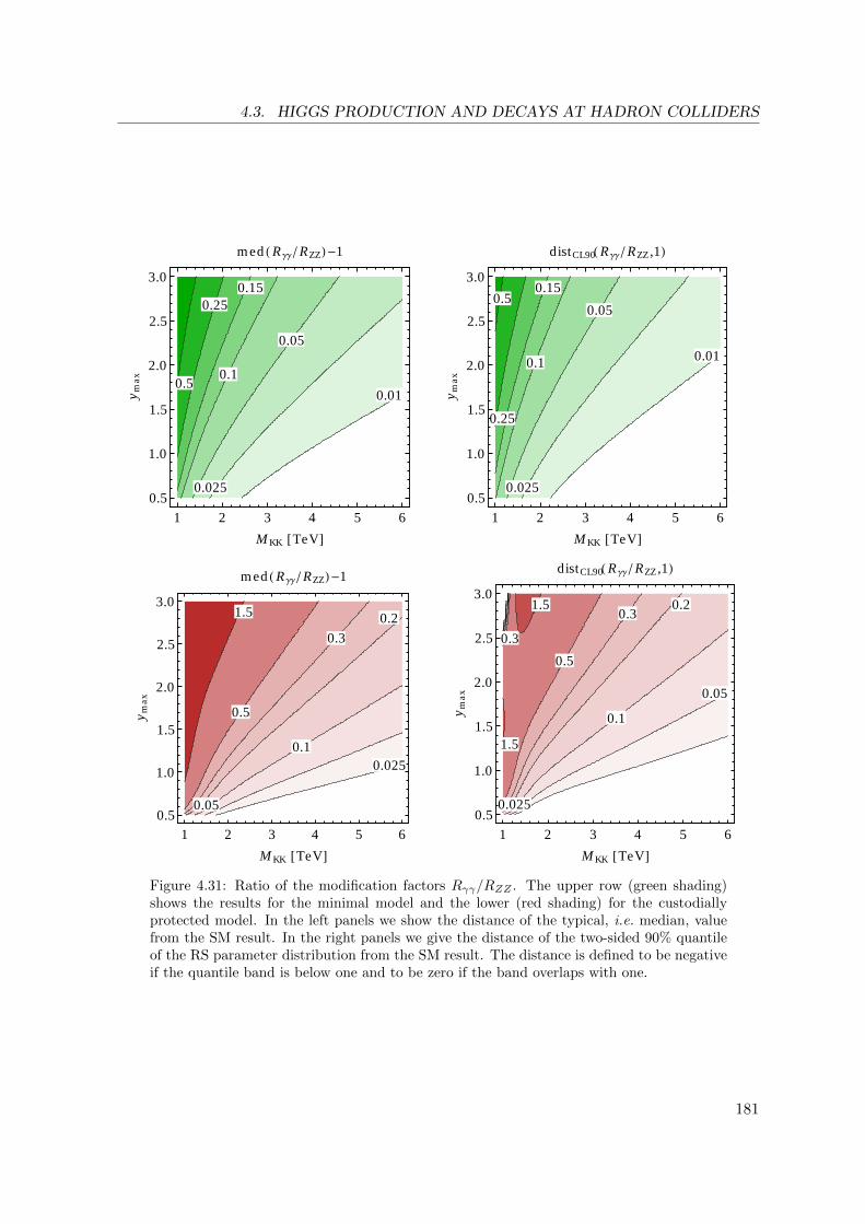
4.3. HIGGS PRODUCTION AND DECAYS AT HADRON COLLIDERS
0.01
0.025
0.05
0.1
0.150.25
0.5
1 2 3 4 5 6
0.5
1.0
1.5
2.0
2.5
3.0
MKK @TeV D
y max
medH RΓΓ RZZL -1
0.01
0.025
0.05
0.1
0.15
0.25
0.5
1 2 3 4 5 6
0.5
1.0
1.5
2.0
2.5
3.0
MKK @TeV D
y max
distCL90H RΓΓ RZZ ,1L
0.025
0.05
0.1
0.2
0.3
0.5
1.5
1 2 3 4 5 6
0.5
1.0
1.5
2.0
2.5
3.0
MKK @TeV D
y max
medH RΓΓ RZZL -1
0.025
0.05
0.1
0.20.3
0.3
0.5
1.5
1.5
1 2 3 4 5 6
0.5
1.0
1.5
2.0
2.5
3.0
MKK @TeV D
y max
distCL90H RΓΓ RZZ ,1L
Figure 4.31: Ratio of the modification factors Rγγ/RZZ . The upper row (green shading)shows the results for the minimal model and the lower (red shading) for the custodiallyprotected model. In the left panels we show the distance of the typical, i.e. median, valuefrom the SM result. In the right panels we give the distance of the two-sided 90% quantileof the RS parameter distribution from the SM result. The distance is defined to be negativeif the quantile band is below one and to be zero if the band overlaps with one.
181
4. ASPECTS OF PRECISION PHYSICS
fractions. In this approximation the effect of virtual W -boson exchange is equivalent to theeffect in the decay to γγ.
The Wilson coefficient CγZ,KKW in (4.3.78) incorporates triangle diagrams with charged
KK-boson excitations in the loop, displayed in the upper right corner of figure 4.21. Thiscontribution can be written as
CγZ,KKW =
2πx2W
c2W
∞∑
n=1
~d TW ~χWn (1) ~χWn (1)T ~dW(xWn)2 IWWZ
nn0 AhW(τW (n) , λW (n)
). (4.3.79)
It is again an excellent approximation to evaluate the loop function AhW (τWn , λWn ) in theinfinite mass limit τhW , λ
Wn → ∞. The form factor then becomes 7cw − 11/(6cw) ≈ 4.0. In
(4.3.79) we denoted the overlap integral of KK-W bosons and the Z-boson zero mode byIWWZnn0 . We find
IWWZnn0 =
(2π)3/2
L
1∫
ε
dt
t
[ (~χZ0 (t)
)1
(~χWn (t)
)21
+
(t2w
− sZcw cW
)T~χZ0 (t)
(~χWn (t)
)22
]
=2π
L
1∫
ε
dt
t~χWn (t)T diag
(1, t2w
)~χWn (t) +O
(v2
M2KK
)
=
t2w , custodial RS ∧ n odd
1 , else
+O
(v2
M2KK
).
(4.3.80)
Since the first term in the sum of (4.3.79) is already suppressed by a factor of v2/M2KK, the
computation of CγZ,KKW to this order in principle requires only the knowledge of the overlap
integral to zeroth order. This leads to the very simple result (4.3.80), at which we have arrivedin two steps. In the second line we neglected the modification of the even and odd zero-modeprofile of the Z boson. We then used the fact that also W–W ′ mixing of the two KK-modesof any given KK-level only starts at O(v2/M2
KK). We find that this approximation is in factreasonable in the minimal model, where the universality of IWWZ
nn0 implies that the expression(4.3.79) can be solved with the same calculation like for CKK
W for the γγ final state in (4.3.74)
minimal RS: CγZ,KKW =
1
2
(7 cw −
11
6 cw
)(1− κW
), (4.3.81)
which equals approximately -77% of CKKW given in (4.3.74). The modification of the SM-like
W+W−h-vertex κW was given in (3.3.152).We perform the sum in (4.3.79) numerically and without further approximations, includ-
ing four KK-levels of bosons and extrapolate the higher KK-level contribution from the factor(B.4.3). The extrapolation has the practical effect that it makes the numerical value suitablefor comparison with the approximation (4.3.81), which uses the analytic resummation withthe 5d propagator. We compare values for the exact numerics with the analytic approxi-mation for selected values of MKK in table 4.3. The absolute values in this table are to becompared with the SM amplitude of AhW (τW , λW ) = 5.796. The zero mode RS contributiondominates in all cases and is canceled to approximately one third by the contribution of KKmodes. Both contributions are approximately doubled in the custodial model with PLR sym-metry compared to the minimal model. We observe a fast decoupling with the KK-scale, but
182
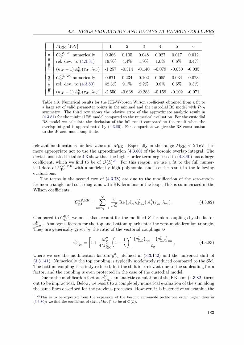
4.3. HIGGS PRODUCTION AND DECAYS AT HADRON COLLIDERS
MKK [TeV] 1 2 3 4 5 6
min
imal
CγZ,KKW numerically 0.366 0.105 0.048 0.027 0.017 0.012
rel. dev. to (4.3.81) 19.9% 4.4% 1.9% 1.0% 0.6% 0.4%
(κW − 1)AhW (τW , λW ) -1.257 -0.314 -0.140 -0.079 -0.050 -0.035
custo
dial
CγZ,KKW numerically 0.671 0.234 0.102 0.055 0.034 0.023
rel. dev. to (4.3.80) 42.3% 9.1% 2.2% 0.8% 0.5% 0.3%
(κW − 1)AhW (τW , λW ) -2.550 -0.638 -0.283 -0.159 -0.102 -0.071
Table 4.3: Numerical results for the KK-W-boson Wilson coefficient obtained from a fit toa large set of valid parameter points in the minimal and the custodial RS model with PLRsymmetry. The third row shows the relative error of the approximate analytic result in(4.3.81) for the minimal RS model compared to the numerical evaluation. For the custodialRS model we calculate the deviation of the full result compared to the result when theoverlap integral is approximated by (4.3.80). For comparison we give the RS contributionto the W zero-mode amplitude.
relevant modifications for low values of MKK. Especially in the range MKK < 2 TeV it ismore appropriate not to use the approximation (4.3.80) of the bosonic overlap integral. Thedeviations listed in table 4.3 show that the higher order term neglected in (4.3.80) has a largecoefficient, which we find to be of O(L)26. For this reason, we use a fit to the full numer-ical data of CγZ,KK
W with a sufficiently high polynomial and use the result in the followingevaluations.
The terms in the second row of (4.3.78) are due to the modification of the zero-mode-fermion triangle and such diagrams with KK fermions in the loop. This is summarized in theWilson coefficients
CγZ,KKq,1 =
∞∑
n=nf+1
v
mqn
Re(gqnn κ
VZ,qn
)Ahq (τqn , λqn) . (4.3.82)
Compared to CKKq,1 , we must also account for the modified Z–fermion couplings by the factor
κVZ,qn . Analogous factors for the top and bottom quark enter the zero-mode-fermion triangle.They are generically given by the ratio of the vectorial couplings as
κVZ,qn =
[1 +
M2Z
4M2KK
(1− 1
L
)] (gqZ,L
)nn
+(gqZ,R
)nn
vq, (4.3.83)
where we use the modification factors gqZ,σ defined in (3.3.142) and the universal shift of(3.3.141). Numerically the top coupling is typically moderately reduced compared to the SM.The bottom coupling is strictly reduced, but the shift is irrelevant due to the subleading formfactor, and the coupling is even protected in the case of the custodial model.
Due to the modification factors κVZ,qn , an analytic calculation of the KK sum (4.3.82) turnsout to be impractical. Below, we resort to a completely numerical evaluation of the sum alongthe same lines described for the previous processes. However, it is instructive to examine the
26This is to be expected from the expansion of the bosonic zero-mode profile one order higher than in(3.3.80): we find the coefficient of (MW /MKK)4 to be of O(L).
183

4. ASPECTS OF PRECISION PHYSICS
structure of (4.3.82) more closely, in order to approximate the KK-lepton contributions, likewe did for the calculation of the γγ final state. To estimate the typical size of CγZ,KK
l,1 , weneed an analytic formula for the relative strength of the vector coupling between the Z bosonand fermionic KK modes in (4.3.82). We find
κVZ,fn = 1−(δF)nn−(δf)nn
vf+O
(m2Z
M2KK
), (4.3.84)
where the elements of the matrices δF,f are of O(1), since fermion mixing is large in KK-levels above the zero-modes. In the fermion embedding of the custodial model with activePLR symmetry, it turns out that for down- and λ-type KK quarks κVZ,fn depends solely onthe electric charge and the third component of the weak isospin of the involved fermions. Weobtain to excellent approximation
κVZ,fn = 1 +T 3 fLL
vf, (f = d, λ) , (4.3.85)
in the custodial model, while no such formula can be derived for up-type quark KK modes orthe fermion embedding of the minimal model. Employing the decoupling limit, τ fn , λ
fn →∞,
i.e. Ahq (τ fn , λfn)→ −1/3, we first derive the expected ratios of
custodial RS: CγZ,KKd,1 ≈ −0.82CKK
d,1 , CγZ,KKλ,1 ≈ −0.28CKK
λ,1 , (4.3.86)
and secondly, that a good conservative estimate for the leptonic contribution is given by
QlvlCγZ,KKl,1
NcQdvdCγZ,KKd,1
≈ Ql(vl + T 3lL )
Qd(vd + T 3dL )
=3− 6s2
w
3− 2s2w
≈ 0.64 . (4.3.87)
Here, we have again assumed a minimal realization of the leptonic embedding in the custodialmodel as described above (4.3.73). We employ the estimate (4.3.87) in the numerical evalua-tion. Admittedly, we cannot resort to such an elegant argument for the minimal RS model.However, in that case we expect the leptonic KK contribution to be negligible. This is due tothe fact that no exotic fermions contribute to fermion mixing in the minimal embedding. Purefermion singlet–doublet mixing renders the diagonal elements of δF and δf to be of similarnumerical size (close to 0.5) in the down sector, where — in contrast to the up sector — noneof the mass splittings is generated by a very strong IR localization of a zero mode fermion.Therefore, we expect the splitting (δF )nn − (δf )nn that enters (4.3.84) to be similarly smallfor leptons. The modified Z–fermion couplings affect (4.3.82) only little; thus, the size of theWilson coefficients (4.3.82) becomes similar for down-quarks and leptons. The small ratio ofvl/vd ≈ 0.11 finally renders the lepton contribution subleading compared to the down-, andcompletely negligible compared to the up-quark contributions.
We show the numerical results for the branching ratio in figure 4.32. There, the EWPOconstraints on the Zbb couplings at 3σ CL are imposed on top of the usual constraints onfermion masses and mixing angles, since the couplings enter one of the contributing diagrams.They EWPO bounds reduce the possible enhancement in the minimal model significantly,from 30% without to 18% after the constraints at MKK = 2.3TeV. In order to obtain a reliablefit result, we exclude the region MKK < 2.3TeV where less than 10% of the parameter pointssurvive the EWPO bounds on the Zbb-couplings. The typical enhancement is 11% at the
184

4.3. HIGGS PRODUCTION AND DECAYS AT HADRON COLLIDERS
Figure 4.32: Fitted modification factor of the branching ratio compared to the SM for thedecay h→ γZ in the minimal and custodial RS model with ymax = 3. The EWPO boundson the Zbb couplings are imposed and curves in the minimal model are only shown for theregion where more than 10% of the parameter space are available. See figure 4.24 for furtherdescriptions.
aforementioned scale. For the custodial model, we observe that both, moderate suppression,and up to large enhancement is possible. However, the typical enhancement is lower than inthe minimal model (only 6% at the aforementioned KK-scale), i.e. typically the contributionsfrom coupling modifications, KK-contributions and the reduction of the total width cancelto a large extent in the final combination. Large modifications are possible for lower valuesof the KK-scale, e.g. up to 60% for MKK = 1.5 TeV. For lower values of ymax the typicalbranching ratios decrease and follow more closely the reduction of the total contribution frombosonic loops. Detailed plots for this case are deferred to the appendix, see figure B.10. Weconclude that a measurement of this decay channel at later stages of the LHC program couldadd valuable information if a pattern of large deviations from the SM should emerge fromthe decay channels that we discussed before. Having said that, we must add that we do notexpect a significant impact on bounds on the KK-scale and the size of the Yukawa matrixelements from a measurement of BR(h→ γZ).
We summarize our extensive discussion on Higgs decay channels with the central insight.The very efficient method to circumvent bounds on the KK-scale from oblique electroweakcorrections by the imposition of a custodial symmetry on the gauge sector also leads tolarger quark multiplicities, which add constructively to the new physics contribution fromthe minimal RS model. Either one realizes fermions in the enlarged gauge symmetry withoutprotecting the b-quark related EWPOs, in which case also a lower bound on ymax and MKK
is active, or one chooses the specific custodial quark embedding presented in section 3.3.5.2,which has an even higher multiplicity due to the exotic quarks with charge 5/3. We foundthat both ways of bypassing EWPO bounds via custodial protection increase the potentialbounds from Higgs physics.
185

186

Chapter 5
Conclusion
A new scientific truth does not triumph byconvincing its opponents and making themsee the light, but rather because itsopponents eventually die, and a newgeneration grows up that is familiar with it.
Max Planck
We conclude this thesis with a summary of its main aspects and results. The commonline of thought was the attempt to improve falsifiability of theories beyond the SM. This isachieved by using dynamical aspects of the models in order to constrain virtual contribu-tions to precisely measured collider observables. One derives constraints on the models, mostfavorably on a common mass scale that determines the predicted resonances. The indirectprocesses we discussed here are known to be usually complementary to astrophysical obser-vations and to collider searches for direct production, due to their inherent dependence onadditional model parameters. This is subject to the given model dynamics. The dynamicscan either be specified completely in a precise model or restricted by a general principle suchas gauge invariance.
We started out with a brief recapitulation of the SM, its symmetry breaking aspects inparticular, and the deficits and open questions it leaves. During the advent of the SM, theorywas following experimental discoveries relatively close. Today, a plethora of models of newphysics has been conceived. Many are motivated by solving some of the theoretical short-comings of the SM; some are just possibilities which are not excluded yet. We showed thatit is worthwhile to practically use the general principle of gauge invariance — or equivalentlyperturbative unitary — as a first classification step. We introduced a generic template La-grangian for this purpose and summarized the constraints from Slavnov-Taylor identities onthe level of Feynman rules. This allows to automatically include unphysical degrees of freedomin a general renormalizable gauge and implies further sum rules between the couplings. Asa proof of concept, we solved the repeatedly emerging task of calculating the flavor changingone-loop penguin amplitude. An example is the FCNC s→ dZ transition that leads to pro-cesses like the rare K → πνν decays. We performed the renormalization and simplificationsof the penguin amplitude by using Slavnov-Taylor identities and gave the full template resultalso for box-type diagrams. We verified the result with the SM and the LHT model. It isan interesting aspect that the Z-penguin amplitude in the LHT model is UV-insensitive dueto the partly gauged symmetry structure, apart from chirally suppressed contributions. As a
187

5. CONCLUSION
byproduct, we simplified results as compared to the literature by introducing a proper vertexdefinition of the CKM matrix.
After this more conceptual part, we presented a full numerical analysis of bounds andcorrelations from flavor observables, electroweak precision observables, and Higgs processesin a specific example, the RS model. This model does not fall into the class of perturba-tively unitary theories. Yet, it shows interesting structure in its couplings that stems fromunique but few assumptions. It provides a theoretically appealing explanation of the gauge-hierarchy problem and quark hierarchies and thus received great interest in the past decade.For our purpose, we found the model to be of interest, since it presently is subject to relevantbounds from observables of all three aforementioned types. Furthermore, there remain un-solved conceptual questions about a proper regularization scheme for the calculation of virtualcorrections in the five-dimensional warped background. We showed that in the calculation ofHiggs processes, subtle questions of limiting procedures in combination with UV regulariza-tion are important in order to obtain correct results. After a careful treatment of these issues,we found that we are not limited by the unsolved questions or remnant UV dependence.
Before performing those calculations, we introduced and discussed in detail the RS modelin a minimal setup with SM-like gauge structure and a setup with custodially protectedgauge symmetry and fermion sector. We did this in a common notation that is extensibleto even more general setups. This was followed by a comprehensive discussion of the KKdecomposition within the mass basis. Paying special attention to Yukawa couplings withnon-standard chirality, the direct treatment in the mass basis allowed to properly accountfor the influence of the δ-function regularization of the IR-localized Higgs boson on the 5dpropagator of fermions. Our approach also has the merit that we were able to summarizethe complete relevant coupling structure for three-point vertices and four-fermion operatorsin a very compact notation. This facilitates the interpretation of the various sources and sizeof contributions when compared to the approach of a 4d decomposition in the electroweakeigenstate basis followed by a re-diagonalization of large mass matrices. Already at thecoupling level, we were able to summarize the differences between the minimal and custodialmodel in terms of a few universal constant factors. We found that, for instance, the left-handedZdidj couplings are suppressed by approximately the inverse volume of the extra dimensionL−1, and the right-handed couplings enhanced by a factor of 3 c2
ws−2w in the custodial compared
to the minimal model. We gave the analogous factors for four fermion couplings, too. TheKK-gluon couplings are the same in both versions of the model and are most important inkaon mixing.
We then began the numerical analyses of the RS model with a discussion of CP violationin kaon mixing. It provides the strongest flavor constraints on the mass scale of the model.Our first main finding was the significant spread in the distribution of the RS predictions,which stems mainly from the dependence on the Yukawa sector. We quantified this andderived new bounds from the lower edge of the resulting distribution by carrying out detailednumerical parameter scans. We found for the first KK-gluon mass — viz. 2.45 times the KKscale — MG(1) > 4.4 TeV, if we request 3% of allowed and non-fine-tuned parameter space atthe 99% CL region. This bound, derived in a rigorous sense, is much weaker than what couldbe expected from the generic order of magnitude enhancement in εK , which is often quotedin the literature. It would lead to MG(1) ≈ 20 TeV, if we request the median to agree withexperiment at the same CL. We found that the aligned case with an SU(3)d flavor-symmetryhelps to lower the bound, but conversely we found a much stronger limit for the little RSmodel due to effects in the UV-region of the bulk. We also considered direct CP violation in
188

K → ππ, i.e. ε′K/εK , which gives an interesting constraint but a much weaker bound on MG(1)
due to large theoretical uncertainties. We noticed that even major theoretical progress will notallow to make this observable a precision constraint on the KK scale. However, ε′K/εK carriesinteresting complementary information, as it enforces the branching ratio of KL → π0νν tobe not larger than twice the SM prediction. We also studied further correlations betweenrare (semi-)leptonic kaon decays that carry information on the chiral structure of the modeland took into account the bounds imposed from εK and ε′K/εK . Additional aspects of ourdiscussion were an outlook for a promising future constraint from Bs → µµ and a discourseof non-standard CKM effects. For the latter, we gave analytical approximate formulas andshowed that effects remain below observable levels. Here, it was necessary to use the four-fermion definition of the CKM and properly take into account the modification of GF . Wealso found a cancellation of contributions in the custodial model, which countervails a possibleenhancement at a lower accessible KK scale. In total, we observed that the severity of the“flavor problem” in the ∆S = 2 sector of warped extra dimensions depends highly on therequired amount of viable parameter space. The KK-scale bounds we gave are now wellcomparable to electroweak precision constraints.
Concerning the EWPOs, we then reviewed up-to-date analyses of the most importantobservables that significantly impact the constraints on models of new physics. We discussedthe choice of input, effective parameters, and Z → bb observables. For the RS model, wereviewed the mechanism of custodial protection in our formalism, which allows to clearlyidentify subleading non-protected contributions. In order to compare the different kindsof bounds in this thesis, we then re-derived the bounds from oblique corrections with theupdated input. We found in the minimal RS model MG(1) > 11.3 TeV, the custodial RSmodel MG(1) > 4.1 TeV, and the LRS model MG(1) > 4.7 TeV at the 3σ CL. Compare thisto the strongest bound obtained from direct searches, which is MG(1) > 1.8 TeV at the 2σCL (see section 4.1.2.1). We also assessed the parameter dependence of the constraints fromZ → bb on the 5d bulk masses of the b quark.
The final part was then committed to Higgs production and decay modes. After a reviewof the SM results, the experimental status, and contributions from additional fermions in thesimple example of the LHT model, our main focus was then to determine the analytical andnumerical structure of the effects in the RS model. Our aim was to discuss the subtle issueof convergence of loop integrals, and the potential on constraining the parameter space.
We derived the RS one-loop contributions to Higgs-boson production via gluon–gluonfusion by a resummation of all KK-fermion-triangle diagrams. The calculation had a conver-gent result. We traced the origin of this non-trivial convergence and observed a cancellationbetween contributions of different chiralities for the vector-like KK fermions. We obtainedanalytic results for the minimal and custodial RS model and showed how to extend it to moregeneral fermion embeddings. As an important aspect, we observed the cancellation of almostall bulk-mass dependence in the result, leading to a simpler prediction. However, we alsorecognized that the limits of the δ-function localization of the IR-brane Higgs boson and theinfinite KK summation do not commute. They lead to O(1) different results depending onthe order of limits. We were able to ascribe this behavior to contributions from ultra-heavyKK modes with masses in a broad region around a new scale Mweak/η. η 1 determinesthe small localization of the regularized Higgs boson near the IR brane, and is eventuallytaken to zero at the end of the calculation. At the scale Mweak/η, the cancellation betweendifferent chiralities is suspended. We detected logarithmic growth of the ggh amplitude inthe summation of many KK-modes around this scale. We demonstrated this explicitly for
189
5. CONCLUSION
the case of a single generation. A solution to this issue was given by the third regularizationthat is present in the problem. Any UV regulator, e.g. cut-off, or dimensional regularization,implies that the ultra-heavy fermion contributions are absent in a full calculation of the 5damplitude.
With the finite UV-insensitive result, we were then able to discuss all leading Higgs-boson-production and decay modes. Besides the KK scale, the most important parameter is given bythe maximal possible values of the 5d Yukawa matrix elements, which are naturally of O(1).We also considered reduced values of ymax, and showed important results in the plane MKK –ymax. Concerning the production modes, we found a very strong suppression of gluon–gluonfusion. A suppression is also present in weak boson fusion, and the associated W , Z, and ttproduction modes. Concerning the subsequent decays, a strong reduction and spread of thetotal width was found to be due to the corrections in h→ bb, if ymax is of natural size.
We found an interesting interplay of modifications for lower than natural Yukawa valuesin the final branching ratios of h → ZZ and h → bb, which maintains a certain constrainingpotential in this region of parameter space. For gg → h → ZZ, we were able to derive arelevant bound at 95% CL. In the custodial model we found MG(1) /∈ [4.8, 9.1] TeV for naturalYukawa values, while for one order of magnitude reduced values we obtained MG(1) > 2.8 TeV.In the minimal model we derived MG(1) > 4.7 TeV for natural Yukawa entries.
The modifications in h→ γγ follow from an interplay of a reduced WWh coupling, whichis partially neutralized by positive KK-W contributions, and moreover exceeded by positivecontributions from the top-Yukawa modification and from KK-fermions. In spite of the can-cellations, we found a large possible enhancement for natural Yukawa values, particularlyfor the custodial model as it features exotic fermions of charge 5/3. Conversely, we found areduction for the case of Yukawa entries that are reduced one order of magnitude below theirnatural size. In combination with the reduced production channels, we derived the boundMG(1) > 2.6 TeV in the minimal and MG(1) > 4.0 TeV in the custodial model at 95% CL. Weargued that no unfolding is necessary due to similar reductions in the relevant productionchannels. In total, we saw that the custodial model with MG(1) . 4.8 TeV and natural Yukawavalues can be compatible even with present central values of the signal strengths.
We then emphasized that the spread of production and width drops in the ratio of signalstrengths of the decay to ZZ and γγ. This ratio could unfold its full constraining potentialof around 11 TeV on MG(1) in the case that the measurements would settle at SM values.
Finally, we also investigated all modifications of the decay into γZ. We derived expressionsthat properly take into account the modified Z couplings, as compared to the decay to γγ.We found that up to 50% enhancement is possible in the custodial model, but less than 20%in the minimal model. This observable could be useful after the LHC upgrade and at highintegrated luminosity.
We close this thesis with re-emphasizing that Higgs physics has reached the turning pointin making the transition from discovery to precision physics in an astonishingly short amountof time. Already now, it provides additional bounds on new physics and the RS model inparticular. We found that bypassing the strong EWPO bounds on the KK scale of the minimalRS model via custodial protection increases the potential bounds from Higgs physics. A smallwindow of MG(1) ∈ [4.4, 4.8] TeV remains open for natural versions of the custodial setup aftertaking into account all the bounds described above. We hope that Higgs physics will soon beable to close this window.
190
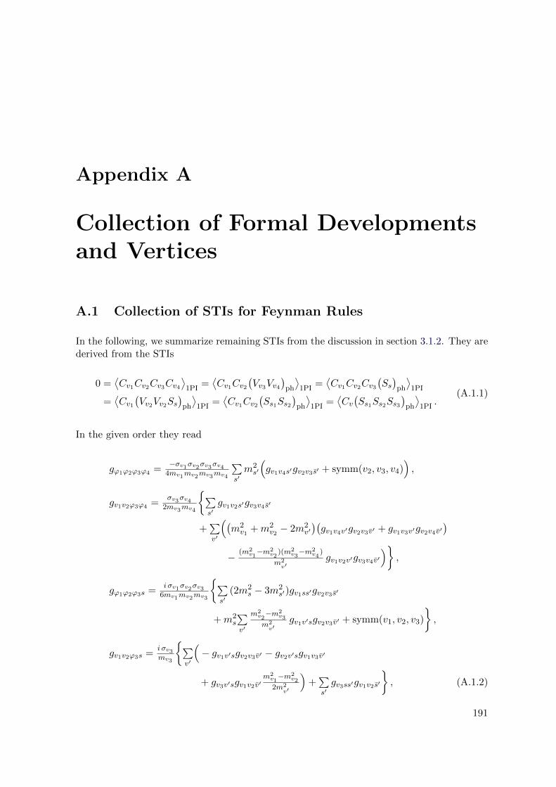
Appendix A
Collection of Formal Developmentsand Vertices
A.1 Collection of STIs for Feynman Rules
In the following, we summarize remaining STIs from the discussion in section 3.1.2. They arederived from the STIs
0 =⟨Cv1Cv2Cv3Cv4
⟩1PI
=⟨Cv1Cv2
(Vv3Vv4
)ph
⟩1PI
=⟨Cv1Cv2Cv3
(Ss)
ph
⟩1PI
=⟨Cv1
(Vv2Vv2Ss
)ph
⟩1PI
=⟨Cv1Cv2
(Ss1Ss2
)ph
⟩1PI
=⟨Cv(Ss1Ss2Ss3
)ph
⟩1PI
.(A.1.1)
In the given order they read
gϕ1ϕ2ϕ3ϕ4 =−σv1σv2σv3σv4
4mv1mv2mv3mv4
∑s′m2s′
(gv1v4s′gv2v3s′ + symm(v2, v3, v4)
),
gv1v2ϕ3ϕ4 =σv3σv4
2mv3mv4
∑s′gv1v2s′gv3v4s′
+∑v′
((m2v1
+m2v2− 2m2
v′)(gv1v4v′gv2v3v′ + gv1v3v′gv2v4v′
)
− (m2v1−m2
v2)(m2
v3−m2
v4)
m2v′
gv1v2v′gv3v4v′
),
gϕ1ϕ2ϕ3s =i σv1σv2σv3
6mv1mv2mv3
∑s′
(2m2s − 3m2
s′)gv1ss′gv2v3s′
+m2s
∑v′
m2v2−m2
v3
m2v′
gv1v′sgv2v3v′ + symm(v1, v2, v3)
,
gv1v2ϕ3s =i σv3mv3
∑v′
(− gv1v′sgv2v3v′ − gv2v′sgv1v3v′
+ gv3v′sgv1v2v′m2v1−m2
v2
2m2v′
)+∑s′gv3ss′gv1v2s′
, (A.1.2)
191

A. COLLECTION OF FORMAL DEVELOPMENTS AND VERTICES
gϕ1ϕ2s1s2 =σv1σv2
2mv1mv2
∑s′
(gs1s2s′gv1v2s′
+[gv1s1s′gv2s2s′ (2m
2s′ −m2
s1 −m2s2) + symm(s1, s2)
])
+∑v′
(gv′s1s1gv1v2v′
(m2s1 −m2
s2
) m2v1−m2
v2
m2v′
+[gv1v′s2gv2v′s1
(m2s1 +m2
s2
)1
4m2v′
+ symm(v1, v2)])
,
gϕs1s2s3 = i σvmv
∑s′gs1s2s′gvs3s′ −
∑v′gv′s1s2gvv′s3
m2s1−m2
s2
2m2v′
+ symm(s1, s2, s3)
.
All rules given here and in section 3.1.2 hold in the limiting case of any of the particlesbeing massless. The couplings of photons or gluons of course simplify considerably and canbe expressed by using the U(1) and SU(3) charges defined in (3.1.1). Moreover, they can beseparated into two classes: Couplings that involve another massive gauge boson and thosewithout. Couplings of the latter class are either directly included in the covariant kineticLagrangian or zero. This includes1
gAϕ1ϕ2 = gAAϕ1ϕ2 = gAϕ1s1 = gAAϕ1s1 = 0 ,
gAAϕ1ϕ2 = −2i(gAv1v1)2δv1v2 .(A.1.3)
The equations also hold with G instead of A. The class of couplings with another massivegauge boson has to be derived from the STIs. They are given by
gAv1ϕ2 = iemv1δv1v2 ,
gAv1ϕ2ϕ3 = e σv2σv3
(Qv2 −Qv3
) m2v2
+m2v3−m2
v12mv2mv3
gv1v2v3 ,
gAv1ϕ2s = −ie σv2
(Qv2 −Qs
)1
2mv2gv1v2s ,
gAv1v2v3 = −e (Qv2 −Qv3) gv1v2v3 ,
gAvs1s2 = e (Qs1 −Qs2) gvs1s2 .
(A.1.4)
We used charge conservation to simplify the right-hand side for the quartic couplings. Thecorresponding equations with a gluon are
gabcGv1ϕ2= iσv2
(T av2
)bcmv1δv1v2 ,
gabcdGv1ϕ2ϕ3= σv2σv3
m2v2
+m2v3−m2
v12mv2mv3
∑c′
((T av2
)cc′gbc′d
v1v2v3−(T aVa3
)dc′gbcc
′v1v2v3
),
gabcdGv1ϕ2s = −i σv21
2mv2
∑c′
((T av2
)cc′gbc′d
v1v2s −(T as)dc′gbcc
′v1v2s
),
gabcdGv1v2v3= −∑
c′
((T av2
)cc′gbc′d
v1v2v3−(T av3
)dc′gbcc
′v1v2v3
),
gabcdGvs1s2 =∑c′
((T as1)cc′gbc′d
vs1s2 −(T as2)dc′gbcc
′vs1s2
).
(A.1.5)
1To derive the vanishing couplings with physical scalars, one has to note that gAv1s2 = 0. This couplinghas to come from the kinetic term of a multiplet Φ under the full gauge group. Thus, it is proportional toeQΦAµV
µa (Φ†TVaΦ). The Goldstone directions are given by TVa〈Φ〉, so they cannot contain physical scalars.
192

A.2. FORMULAS AND VERTICES OF THE LITTLEST HIGGS MODEL
For completeness, we remark that the ghost couplings can be derived by inserting anotheroff-shell gauge boson in the derivation of (3.1.11). Following the derivations in [132, 133] oneuses the BRST variation sV µ
v1(x) = ∂µVv1(x) + i(gf)v1v2v3Vµv2(x)uv3(x), where (gf)v1v2v3 are
the structure constants times corresponding couplings, rotated into the mass basis. Since thelatter are per se unknown in our generic Lagrangian (3.1.2), which is already given in themass basis, one removes the contact term again by considering connected Green’s functionsonly. In this way, one can derive gsu1u2 = −1
2 gv1v2s and gv3u1u2 = gv1v2v3 . The index set forghosts agrees with the one for gauge bosons, analogous to the indices for Goldstone bosons.The latter relation for gauge-boson couplings to ghost currents is already clear, since the samerotations are applied to gauge bosons and ghosts when going to the mass basis. Hence, wehave reconstructed all unphysical couplings that are necessary for one-loop calculations in ageneral Rξ gauge.
A.2 Formulas and Vertices of the Littlest Higgs Model
In this appendix we summarize some of the remaining relations for the LH model and theFeynman rules for the vertices in the model with T -parity.
In the Lagrangian, the kinetic terms for gauge bosons take the standard form. We rewritethem in terms of the SM-like gauge eigenstates. Using with charge eigenstates and ε+− 3 = 1we obtain
LV = −1
4
∑
j=1,2
( ∑
a=1,2,3
W aj µνW
aµνj +Bj µνB
µνj
)
= −1
4
( ∑
a=+,−,3
∣∣∂µW aν − ∂νW a
µ + igεabc(W bµW
cν +W ′bµW
′cν )∣∣2
+∑
a=+,−,3
∣∣∂µW ′aν − ∂νW ′aµ + igεabc(W ′bµWcν −W ′bν W c
µ +δgcsW
′bµW
′cν )∣∣2
+∣∣∂µBν − ∂νBµ
∣∣2 +∣∣∂µB′ν − ∂νB′µ
∣∣2).
(A.2.1)
The full redefinition of scalars, necessary to bring (3.2.16) and (3.2.17) into canonical formas discussed in the main text, is given by
(hmφ0m
)=
1− v
2
f2
x2λ4
vfxλ√
2
− vfxλ√
21− v2
12f2
(1+3x2
λ
)
(hφ0
),
φPmπ0m
ηmω0m
=
1− v2
12f2
(1+3x2
λ
)− v√
2fxλ −
√5v2
6√
2f2 − v2
6√
2f2
v√2fxλ 1− v2
12f2 r22
√5v
2f δg′v
2f δg√5v2
3√
2f2
(1−3
2 δg′xλ
)−√
5v2f δg′ 1− 5v2
24f2
(1+3δ2
g′
)−√
5v2
6f2
(1−6xHc
′s′
twcs
)
v2
3√
2f2
(1−3
2 δgxλ
)− v
2f δg −√
5v2
6f2 r42 1− v2
24f2
(1+3δ2
g
)
φP
π0
ηω0
,
r22 =(
1 + 32
(δ2g + 5δ2
g′)
+ 3x2λ
), r42 =
(1 +
3twxH(1−δ2g)
10cc′ss′
),
193

A. COLLECTION OF FORMAL DEVELOPMENTS AND VERTICES
φ±mπ±mω±m
=
1− 124
v2
f2 (1+3x2λ) −1
2vf xλ − 1
12v2
f2
12vf xλ 1− 1
12v2
f2
(1+
32 (δ2
g+x2λ))
12 δg
vf
16v2
f2
(1−3
2 δgxλ
)−1
2vf δg 1− 1
24v2
f2 (1+3δ2g)
φ±
π±
ω±
. (A.2.2)
In the following, we summarize all non-zero three-point couplings of physical particles in themodel with T -parity. We derived them by implementing the full Lagrangian in a computeralgebra system, with which we applied the functional derivatives and the necessary Taylorexpansions in v/f . The triple vector couplings, including v4/f4 corrections, are given by
gW+W−
(AZ
) = gW+HW
−H
(AZ
) = g(−swcw
), (A.2.3)
gW+W−H
(AHZH
) = g
v2
f2xH
(1 + v2
f2
(14 + 2xH
3cwsw
))
1− v4
f4
x2H2
. (A.2.4)
For the couplings of two vectors and one scalar we omit corrections of order v3/f3, if a scalarrotation beyond the order included in (A.2.2) would contribute. We always keep track of themaximal reliable order in all vertices we derived. The resulting v2/f2, and parts of the v3/f3
corrections are given by
(gZZh
gW+W−h
)= g2v
2
(1− v2
3f2
)(c−2w
1
),
gAHAHhgAHZHhgZHZHhgW+
HW−Hh
= −g2v
2
t2w
(1− v2
f2
(43 − 2
twxH))
tw
(1− v2
f2
(43 +
(tw − 1
tw
)xH))
1− v2
f2
(43 + 2twxH
)
1− v2
f213
+O(v3
f3
),
gZ(AHZH
)φ0
= − g2v
2√
2 cw
vf
(1− v2
f2
(512 −
xHtw
))(tw1
),
gZW+
Hφ−
gW+AHφ−
gW+ZHφ−
= g2v
4vf
1cwtw1
+O
(v3
f3
), gAW+
Hφ− = O
(v3
f3
),
gW+W+Hφ−− = −g2v
2vf
(1− v2
6f2
), gW+W−Hφ
P = i g2v
45√
2v3
f3 .
(A.2.5)
For the scalar–scalar–vector couplings there exists a second Lorentz-structure with Feynmanrules proportional to the sum of the scalar momenta p2 + p3 instead of the difference p2− p3,
194

A.2. FORMULAS AND VERTICES OF THE LITTLEST HIGGS MODEL
whose coupling we denote by g+. The complete set of couplings is given by
gAφ+φ− = gAφ++φ−−/2 = −gsw ,
gZφ0φP
gZφ+φ−
gZφ++φ−−
= g
cw
i(
1− v2
4f2
)
−(s2w − v2
8f2
)
1− 2s2w
,
gW+φ0φ− g+
W+φ0φ−
gW+φPφ− g+W+φPφ−
gW+φ+φ−− g+W+φ+φ−−
= g
1/√
2
i/√
21
(
1− v2
8f2 , − v2
12f2
),
(gAHhφP /tw g+
AHhφP/tw
gZHhφP g+ZHhφP
)= − ig
2√
2vf
(1 + v2
f2
(512 ±
xHtw
), −1
3
[1− v2
f2
(760 ∓
xHtw
)]),
(gW+
Hhφ− g+
W+Hhφ
−
)= −g
4vf
(1 + v2
24f2 ,−13
[1− 11
120v2
f2
]).
(A.2.6)
To denote the couplings of fermions, we use T3,uH ≡ T3,u = 1/2 and T3,dH ≡ T3,d = −1/2. Forthe heavy fermions, these are not to be interpreted as charges, but only defined for notationalconvenience. The vertex definition of the CKM matrix Vij in terms of the unitary matrix Vij ,which is part of the diagonalization of the fundamental mass matrix, was given in (3.2.29).We also abbreviate xL ≡ xL/V33. The couplings of vectors to fermion currents are given by
g(LR)Aff
= −gswQf ,
g(LR)Zff
= gcw
((T3f−Qf s2w−Qf s2w
)− v2
8f2
(4x2L(δf,t−δf,T+
)
δf,uH+δf,νH
)),
gLZtT+= v
fg
2cwxL
(1 + v2
2f2
(2d2 − x2
L
)),
gLW+uidj= g√
2Vij , gLW+νiej
= g√2
(VPMNS
)ij,
gLW+T+dj= v
fg√2xL
(1 + v2
2f2
(2d2 + x2
L
))V3j ,
g(LR)W+uH,idH,i
= gW+νH,ieH,i = g√2
(1
1− v2
8f2
),
(A.2.7)
gL(AHZH
)fH,ifj
= g2
((tw/52T3,f
)+(
2T3,f
−tw/5
)v2
f2xH
)(VHf
)ij,
gL(AHZH
)uH,iT+
= vfg2 xL
((tw/5
1
)(1 + v2
2f2
(2d2 + x2
L
))+(
1−tw/5
)v2
f2xH
)(VHu
)i3,
g(LR)AH T−(t,T+)
= 25g tw
vf xL
(1+
v2
f2 d2
)−(
1− v2
2f2 x2L
),
√xL
(1− v2
2f2 (1−xL)(
1−2x2L
))−√1−xL
(1+
v2
2f2 xL
(1−2x2
L
)) ,
g(LR)ZH T−(t,T+)
= 25gtwxH
(− v
3
f3 xLv2
f2
− v2
f2√xL
v2
f2
√1−xL
),
195
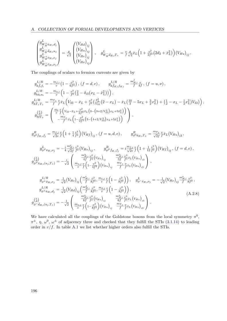
A. COLLECTION OF FORMAL DEVELOPMENTS AND VERTICES
gLW+H uH,idj
gLW−H dH,iuj
gLW+H νH,iej
gLW−H eH,iνj
= g√2
(VHd
)ij(
VHu)ij(
VHe)ij(
VHν)ij
, gL
W−H dH,iT+= v
fg√2xL
(1 + v2
2f2
(2d2 + x2
L
))(VHu
)ij.
The couplings of scalars to fermion currents are given by
gL/R
hfifi= −mf,i
v
(1− v2
6f2
), (f = d, e) , g
L/R
hfH,ifH,i=
mfH,if
v4f , (f = u, ν) ,
gL/Rhuiui
= −mu,iv
(1− v2
f2
(23 − δi3
(xL − x2
L
))),
gL/R
hT+T+=
mT+
fvf xL
(V33 − xL + v2
f2
( x2L
V33
(2− xL
)− xL
(103 − 5xL + 3
2x2L
)+(
12 − xL − 1
2x2L
)V33
)),
g(LR)htT+
=
mtvvf
(V33−xL+
v2
2f2 xL
(3−(
3+2/V 233
)xL+5x2
L
))
−mT+
f xL
(1− v2
2f2
(3−(
4+2/V 233
)xL+5x2
L
)) ,
gRφ0fH,ifj=
mf,j√2v
vf
(1 + 1
4v2
f2
)(VHf
)ij, (f = u, d, e) , gRφ0uH,iT+
=mT+√
2fvf xL
(VHu
)i3,
gLφP νH,iνj = − i4
mνH,i√2f
v2
f2
(VHν
)ij, gRφP fH,ifj = i
mf,j√2v
vf
(1 + 1
12v2
f2
)(VHf
)ij, (f = d, e) ,
g(LR)φP uH,i(uj ,T+)
= − i√2
muH,i4f
v2
f2
(VHu
)ij
muH,i3f
v3
f3 xL
(VHu
)i3
mu,jv
vf
(1− v2
4f2
)(VHu
)ij
mT+
fvf xL
(VHu
)i3
,
gL/Rφ+νH,iej
= 1√2
(VHe
)ij
(meH,if
v2
8f2 ,me,jv
vf
(1− v2
8f2
)), gLφ−eH,iνj = − 1√
2
(VHν
)ij
mνH,if
v2
8f2 ,
gL/Rφ+uH,idj
= 1√2
(VHd
)ij
(mdH,if
v2
8f2 ,md,jv
vf
(1− v2
8f2
)),
g(LR)φ−dH,i(uj ,T+)
= − 1√2
muH,i8f
v2
f2
(VHu
)ij
muH,i6f
v3
f3 xL
(VHu
)i3
mu,jv
vf
(1− v2
8f2
)(VHu
)ij
mT+
fvf xL
(VHu
)i3
.
(A.2.8)
We have calculated all the couplings of the Goldstone bosons from the local symmetry π0,π±, η, ω0, ω± of adjacency three and checked that they fulfill the STIs (3.1.14) to leadingorder in v/f . In table A.1 we list whether higher orders also fulfill the STIs.
196

A.2. FORMULAS AND VERTICES OF THE LITTLEST HIGGS MODEL
fv 1 v
fv2
f2v3
f3
g(A,Z)W+π− + +
g(A,Z)W+Hω− , gZHW+ω− + + u
gAHW+ω− , gZH ,W+H ,π
− + u
gW+W−Hω0 + + x
gAHW+Hπ− + x
gW+W−H η+ x
g(A,Z)π+π− , gW+π0π− +
gZω+ω− , gW+ω0ω− + +gW+ηω− +gZHπ+ω− , gW+
Hπ0ω− , gW+
H ,π−,ω0 + +
gAHπ+ω− , gW+Hπ−η + x
gZπ0h, gW+π−h + +gZ(η,ω0)φ0 , gZω+φ− , gW+(η,ω0)φ− , gW+ω+φ−− +
g(AH ,ZH)π0φ0 , g(AH ,ZH)π+φ− , g(AH ,ZH)(η,ω0)h, . . .
. . . gW+Hπ
0φ− , gW+Hπ
+φ−− , gW+Hω−h
+ +
gW+Hπ−φP x
gL,Rπ0fifi
(f = u, d, e), gL,Rπ+uidj
, gL,Rπ+νiej
, gLπ0T+t
, gLπ+T+dj
+ +
gRπ0T+t
, gRπ+T+dj
+ +
gL,Rπ0T+T+
+ x
gπ0uH,iuH,i , gπ0νH,iνH,i , gπ+uH,idH,i , gπ+νH,ieH,i (all = 0) x
gL(η,ω0)fH,ifj
, (f = d, e) + +
gR(η,ω0)fH,ifj
, (f = d, e) + x
gL(η,ω0)fH,ifj
, (f = u, ν) + x
gR(η,ω0)uH,iuj, gL(η,ω0)uH,iT+
+ +
gR(η,ω0)uH,iT++ x
gLη(ui,T+)T−
+ +
gLω0(ui,T+)T−
+
gLω−uH,i,dj , gLω−,−νH,i,ej + +
gRω−uH,i,dj , gRω−,−νH,i,ej + +
gLω+dH,i,uj
, gLω+,−eH,i,νj + x
gRω+dH,i,uj
, gLω+dH,i,T+
+ +
gRω+dH,i,T+
+ x
Table A.1: Check of STIs (3.1.14) for the LHT model and linear gauge fixing. Entries areonly given at the orders that are present in the couplings. A “+” indicates the couplingfulfills the STI at the given order, an “x” if otherwise, and a “u” if we cannot derive it, e.g.because of missing scalar rotations at the given order.
197
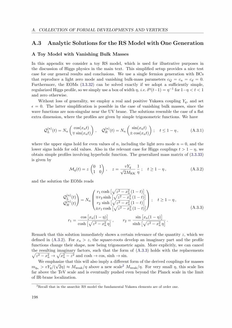
A. COLLECTION OF FORMAL DEVELOPMENTS AND VERTICES
A.3 Analytic Solutions for the RS Model with One Generation
A Toy Model with Vanishing Bulk Masses
In this appendix we consider a toy RS model, which is used for illustrative purposes inthe discussion of Higgs physics in the main text. This simplified setup provides a nice testcase for our general results and conclusions. We use a single fermion generation with BCsthat reproduce a light zero mode and vanishing bulk-mass parameters cQ = cu = cd = 0.Furthermore, the EOMs (3.3.32) can be solved exactly if we adopt a sufficiently simple,regularized Higgs profile, so we simply use a box of width η, i.e. δη(t−1) = η−1 for 1−η < t < 1and zero otherwise.
Without loss of generality, we employ a real and positive Yukawa coupling Yq, and setε = 0. The latter simplification is possible in the case of vanishing bulk masses, since thewave functions are non-singular near the UV brane. The solutions resemble the case of a flatextra dimension, where the profiles are given by simple trigonometric functions. We have
Q(n)L (t) = Nn
(cos(xnt)∓ sin(xnt)
), Q(n)
R (t) = Nn
(sin(xnt)± cos(xnt)
); t ≤ 1− η , (A.3.1)
where the upper signs hold for even values of n, including the light zero mode n = 0, and thelower signs holds for odd values. Also in the relevant case for Higgs couplings t > 1 − η, weobtain simple profiles involving hyperbolic function. The generalized mass matrix of (3.3.33)is given by
Mq(t) = z
(0 11 0
), z =
vYq√2MKK
1
η; t ≥ 1− η , (A.3.2)
and the solution the EOMs reads
(Q(n)L (t)
Q(n)R (t)
)= Nn
r1 cosh[√
z2 − x2n (1− t)
]
∓r2 sinh[√
z2 − x2n (1− t)
]
r2 sinh[√
z2 − x2n (1− t)
]
±r1 cosh[√
z2 − x2n (1− t)
]
; t ≥ 1− η ,
r1 =cos[xn(1− η)
]
cosh[√
z2 − x2n η] , r2 =
sin[xn(1− η)
]
sinh[√
z2 − x2n η] .
(A.3.3)
Remark that this solution immediately shows a certain relevance of the quantity z, which wedefined in (A.3.2). For xn > z, the square-roots develop an imaginary part and the profilefunctions change their shape, now being trigonometric again. More explicitly, we can cancelthe resulting imaginary factors, such that the form of (A.3.3) holds with the replacements√z2 − x2
n →√x2n − z2 and cosh→ cos, sinh→ sin.
We emphasize that this will also imply a different form of the derived couplings for massesmqn > vYq/(
√2η) ≈ Mweak/η above a new scale2 Mweak/η. For very small η, this scale lies
far above the TeV scale and is eventually pushed even beyond the Planck scale in the limitof IR-brane localization.
2Recall that in the anarchic RS model the fundamental Yukawa elements are of order one.
198

A.3. ANALYTIC SOLUTIONS FOR THE RS MODEL WITH ONE GENERATION
The mass eigenvalues xn are determined by matching the profile functions at t = 1− η
tan[xn(1− η)
]=
±√z ∓ xnz ± xn
tanh[√
z2 − x2n η], xn < z ,
−√xn ∓ zxn ± z
tan[√
x2n − z2 η
], xn > z .
(A.3.4)
These equations can easily be solved numerically. For the normalization factors we obtain
N−2n = 1 +
z
z2 − x2n
[± 1
2sin[2xn(1− η)
]− η(z ∓ xn cos
[2xn(1− η)
])]. (A.3.5)
Using these results, it is not difficult to calculate the relevant overlap integrals with the Higgsprofile. After a series of elementary simplifications we arrive at
gRhqnqn =mn
vN2n
z
z2 − x2n
[± 1
2sin[2xn(1− η)
]− η(z ∓ z2
xncos[2xn(1− η)
])]
=mn
v
[1−N2
n
(1∓ ηz
xncos[2xn(1− η)
])],
(A.3.6)
for the coupling of two fermions of equal KK level to the Higgs boson. Again the upper andlower signs correspond to odd and even KK level. The expression is valid for all regions, bothxn < z and xn > z. To demonstrate how the different form of the profiles is reflected inthe value of the couplings, we approximate the result in three regions, always neglecting thecorresponding small mass ratio and relative O(η) corrections.
1) xn z : We observe the typical equidistant spacing of masses given by the solutions to
tan2(xn) = tanh2(yq) ; yq =vYq√2MKK
, . (A.3.7)
The zero mode has mass x0 = arctan(
tanh(yq))
and the following masses are given by
xn =
n2 π + x0 , n evenn+1
2 π − x0 , n odd. (A.3.8)
The couplings of the two KK modes in a given KK level are of opposite sign
gRhqnqn = ± Yq√2
1
cosh(2Xq). (A.3.9)
2) xn ≈ z : In this region we set xn = z(1 + ζn) and use ζn as an expansion parameter. We observefrom the characteristic equation
tan(xn(1− η)) = −yq
O(ζn) , n even
2 +O(ζn) , n odd, (A.3.10)
that the spacing between KK levels is approximately equidistant. However, there arerelevant changes in the Higgs–fermion couplings. Over a broad range around xn ≈ z
199

A. COLLECTION OF FORMAL DEVELOPMENTS AND VERTICES
they grow with increasing KK level for fermions of both even and odd BCs, i.e. even andodd n. They both eventually reach individual maxima, where also the odd couplingshave turned positive. We expand the characteristic equation and the odd couplingslinearly in ζn, in order to verify the zero crossing analytically and found that
gRhqnqn∣∣n odd
≈ 0 , at ζn =1
4y2q
+O(y0q ) . (A.3.11)
Similarly, by expanding to third order in ζn, we found the maximal value for the evencoupling
gRhqnqn∣∣n even
≈ yq(
1 + 23y
2q +O(y4
q )), at ζn = 1 +O(y2
q ) . (A.3.12)
Remark that the power series in ζn gives good results even for ζn > 1, since higherorders in ζn also come with additional powers of yq. The results (A.3.11) and (A.3.12)thus reproduce the numerical results with a good quality.
3) xn z : Approximately equidistant spacing is still preserved by the characteristic equation
tan2(xn(1− η)) = tan2(xnη) . (A.3.13)
The couplings of both chirality types stay positive, but undergo a damped oscillationwith increasing KK level. We verify this numerically in section 4.3.3 of the main text.
Stability under Variations of the Bulk Masses
The states with xn z, called case 1) in the last section, are of physical interest. We argue inthe main text, that the heavy resonances — cases 2) and 3) — will be decoupled automaticallyby a proper UV regulation of the theory. Therefore we consider a small variation of the bulkmass parameters δcQ,q under this condition. It is straightforward to derive the characteristicequation for η → 0 and to first order in δcQ,q. It reads
tan2(xn) = y2q + δc
tan(xn)
cos2(xn)Si(2xn) ; yq = tanh(yq) . (A.3.14)
Here, we were allowed to neglect UV brane effects, so again we took the limit ε → 0. Sincethe characteristic equation is symmetric in cQ and cq, both variables have the same coefficientin the linearization, and we set δc ≡ δcQ + δcq. The sine integral in (A.3.14) is defined asSi(z) =
∫ z0 dt sin(t)/t. Denoting the solutions (A.3.8) of the case with vanishing bulk masses
as x(0)n and using (A.3.6) we obtain
xn = x(0)n +
δc
2Si(2xn) ,
∂
∂c
vgRhqnqnmn
∣∣η→0
= − yq1 + y2
q
Si(2x(0)
n
)[±(1− y2
q
)(x(0)n
)−2+ 2yq
(x(0)n
)−1].
(A.3.15)
The variation of the total sum of the last line is indeed zero as we show now. We set ξ ≡ x(0)0 /π
and obtain
∂
∂c
∞∑
n=0
vgRhqnqnmn
= − yq1 + y2
q
(1− y2
q
)[ ∞∑
k=1
(Si(2π(k + ξ))
π2(k + ξ)2− Si(2π(k − ξ))
π2(k − ξ)2
)+
Si(2πξ)(πξ)2]
+ 2yq
[ ∞∑
k=1
(Si(2π(k + ξ))
π(k + ξ)+
Si(2π(k − ξ))π(k − ξ)
)+
Si(2πξ)
πξ
], (A.3.16)
200

A.3. ANALYTIC SOLUTIONS FOR THE RS MODEL WITH ONE GENERATION
where we summed over KK levels k and separated the zero mode contribution that appears asthe last term in each of the square brackets. The expressions inside each square bracket canbe shown to cancel using relations for special functions that can be found e.g. in [444]. Weuse the series expansion of the sine integral, the Hurwitz zeta function ζ, and the followingrelations for the Bernoulli polynomials Bn
Si(z) =
∞∑
m=0
sm z2m+1 , sm =
(−1)m
(2m+ 1) (2m+ 1)!, (A.3.17)
ζ(n, z) =∞∑
m=0
(m+ z)−n , ζ(−n, z) = −Bn+1(z)
n+ 1, n ∈ N0
+ , (A.3.18)
Bn(1− z) = (−1)nBn(z) , Bn(1 + z) = Bn(z) + n zn−1 . (A.3.19)
The sum in the first square bracket in (A.3.16) becomes
∞∑
k=1
(Si(2π(k + ξ))
(k + ξ)2− Si(2π(k − ξ))
(k − ξ)2
)=
∞∑
m=0
sm
∞∑
k=1
((k + ξ)2m−1 − (k − ξ)2m−1
)
= −∞∑
m=0
sm ξ2m−1 = − 1
ξ2Si(2πξ) ,
(A.3.20)
and the other sum is treated analogously. Consequently, the total variation in (A.3.16) van-ishes. In summary we have shown that the total sum
∑n
(v gRhqnqn/mn|η→0
)is stable under
small variations of any of the two bulk-mass parameters. One can in principle continue alongthe same lines for all higher derivatives, where one needs complicated derivatives of the seriesexpansion of the Bessel function with respect to the order parameter, instead of the simplerelations (A.3.17). Since the total sum has no poles and is built of products and quotientsof Bessel functions that are entire functions in the order parameter, such a calculation wouldprove rigorously that the total sum indeed vanishes for all bulk-mass parameters.
201

202

Appendix B
Collection of Numerical andTechnical Details
B.1 Loop Functions
We summarize the loop functions used in section 4.1. Following reference [250] they aredefined with ε = (4−D)/2 as
i
(4π)2B0
(m1,m2
)(4π
µ2e−γE
)ε=
∫dDq
(2π)D1
q2 −m21
1
q2 −m22
,
i
(4π)2C0
(m1,m2,m3
)(4π
µ2e−γE
)ε=
∫dDq
(2π)D1
q2 −m21
1
q2 −m22
1
q2 −m23
, (B.1.1)
i
(4π)2D0
(m1,m2,m3,m4
)(4π
µ2e−γE
)ε=
∫dDq
(2π)D1
q2 −m21
1
q2 −m22
1
q2 −m23
1
q2 −m24
.
These functions read
B0
(m1,m2
)=
1
ε+ 1 +
m21 ln
(µ2
m21
)
m21 −m2
2
+ symm(m1,m2)
,
C0
(m1,m2,m3
)=
m21m
22 ln
(m2
2
m21
)
(m2
1 −m22
)(m2
1 −m23
)(m2
2 −m23
) + symm(m1,m2,m3) , (B.1.2)
D0
(m1,m2,m3,m4
)=
m21 lnm2
1(m2
1 −m22
)(m2
1 −m23
)(m2
4 −m21
) + symm(m1,m2,m3,m4) ,
where the symbol symm(. . .) indicates that one has to sum the preceding terms over all cyclicpermutations of the masses without multiplication of a symmetry factor. We furthermoredefine the combinations of loop functions
C0
(m1,m2,m3
)= B0
(m2,m3
)+m2
1C0
(m1,m2,m3
),
D0(m1,m2,m3,m4) = C0
(m2,m3,m4
)+m2
1D0
(m1,m2,m3,m4
),
(B.1.3)
which arise from the loop integrals (B.1.1) with an additional q2 in the numerator.
203

B. COLLECTION OF NUMERICAL AND TECHNICAL DETAILS
The functions that describe the effects of quark and boson loops in the production anddecay of the Higgs boson are proportional to the so called form factors as introduced inchapter 4.3. The analytic expressions are summarized e.g. in [142]. In our conventions theyare given by
Ahq (τ) =3 τ
2[ 1 + (1− τ) f(τ) ] , Bh
q (τ) = τf(τ) ,
AhW (τ) = −3
4[ 2 + 3τ + 3τ (2− τ) f(τ) ] ,
Ahq (τ, λ) = −I(τ, λ) + J(τ, λ) ,
AhW (τ, λ) = cw
4
(3− s2
w
c2w
)I(τ, λ) +
[(1 +
2
τ
)s2w
c2w
−(
5 +2
τ
)]J(τ, λ)
.
(B.1.4)
The function Bhq for the CP -violating part can be found in [445]. The functions I(τ, λ) and
J(τ, λ), relevant for final states of two different gauge bosons (Zγ), take the form
I(τ, λ) = − τλ
2(τ − λ)
[f(τ)− f(λ)
],
J(τ, λ) =τλ
2 (τ − λ)+
τ2λ2
2 (τ − λ)2
[f(τ)− f(λ)
]+
τ2λ
(τ − λ)2
[g(τ)− g(λ)
],
(B.1.5)
while the functions f(τ) and g(τ) [446] read
f(τ) = arctan2
(1√τ − 1
)=
−1
4
[ln
(1 +√
1− τ1−√
1− τ
)− iπ
]2
, τ ≤ 1 ,
arcsin2
(1√τ
), τ > 1 ,
(B.1.6)
g(τ) =√τ − 1 arctan
(1√τ − 1
)=
1
2
√1− τ
[ln
(1 +√
1− τ1−√
1− τ
)− iπ
], τ ≤ 1 ,
√τ − 1 arcsin
(1√τ
), τ > 1 .
(B.1.7)
B.2 Numerical Input Parameters
Here we collect the numerical values of input parameters used throughout the numericaldiscussion of the RS model. We order them thematically in the following.
Concerning the parameters entering the discussion of EWPOs in section 4.2, we followessentially [344]. We use [69] for the strong coupling constant and the most recent Tevatronaverage of the top-quark mass [447]
GF = 1.1663787(6) · 10−5 GeV−2 , s2w = 0.23116(12) ,
αs(MZ) = 0.1184(7) , ∆α(5)had(MZ) = 0.02757(10) ,
MW = 80.385(15) GeV , MZ = 91.1875(21) GeV , mt = 173.18(94) GeV .
(B.2.1)
204

B.2. NUMERICAL INPUT PARAMETERS
The numerical value of the fine structure constant at MZ is parametrized by the on-shellvalue α(MZ) = α/(1−∆α(MZ)), with the value in the Thomson limit Q2 = 0 being α−1 =137.035999074(44) [69]. The hadronic contribution to ∆α(MZ) is taken from [448]. Unlessnoted otherwise, the reference value for the Higgs-boson mass is Mh = 126 GeV.
In the flavor analyses of section 4.1 we employ the following numerical values:
Parameter Value ± Error Reference
MK 497.614(24) MeV [69]fK 156.1(11) MeV [449]Bsd
1 0.52(2) [274]Bsd
2 0.54(3) [274]Bsd
3 0.94(8) [274]Bsd
4 0.82(5) [274]Bsd
5 0.63(7) [274]ms(2 GeV) 93.4(11) MeV [449]md(2 GeV) 3.41(5) MeV [449]
ϕε 43.52(5) [69]κε 0.94(2) [275]
(∆MK)exp 3.484(6) · meV [69]|εK |exp 2.228(11) · 10−3 [69]mt(mt) 163.6(11) GeV [447]mc(mc) 1.279(1) GeV [450]ηtt 0.5765(65) [327]ηcc 1.87(76) [279]ηct 0.496(47) [451]|Vus| 0.2252(9) [69]|Vcb| 0.0409(11) [69]
Parameter Value ± Error Reference
(ε′K/εK)exp 16.6(23) · 10−4 [69]
B(1/2)6 [0.8, 2.0] [291]
B(3/2)8 [0.8, 1.2] [291]
κL 2.247(13) · 10−10 [302]κ+ 0.5210(25) · 10−10 [302]
∆EM −0.003 [302]Xt 1.469(17) [305]Pc,u 0.41(4) [306–309]
yc −0.20(3) [311]yγγ 0.4(5) [312]yA −0.68(3) [314]
|aS | 1.20(20) [315, 316]yV 0.73(4) [314]
MBd 5.2796(2) GeV [69]MBs 5.3668(2) GeV [69]mµ 105.66 MeV [69]fBd 190.6(47) MeV [449]fBs 227.6(50) MeV [449]τBd 1.525(9) ps [452]
τBs(1.472+0.024
−0.026
)ps [452]
cA 0.96± 0.02 [303, 304]
In the numerical analysis of the RS model we generated parameter points and checkedtheir validity by requiring the fermionic spectrum to comply with the following values of MSquark masses evaluated at the scale MKK = 1 TeV
mu = (1.5± 1.0) MeV , mc = (560± 40) MeV , mt = (144± 5) GeV ,
md = (3.0± 2.0) MeV , ms = (50± 15) MeV , mb = (2.3± 0.1) GeV .(B.2.2)
They correspond to the low-energy values as compiled in [453]. The central values and errorsof the Wolfenstein parameters are taken from [454] and read
λ = 0.2255± 0.0009 , A = 0.807± 0.018 , ρ = 0.147+0.029−0.017 , η = 0.343± 0.016 . (B.2.3)
The requirements on the data sets of RS points are the same as used in [3] and were notupdated here. Small variations (within error ranges) of the values in (B.2.2) and (B.2.3) areirrelevant, as they affect only the RS contributions and not the leading SM values.
205
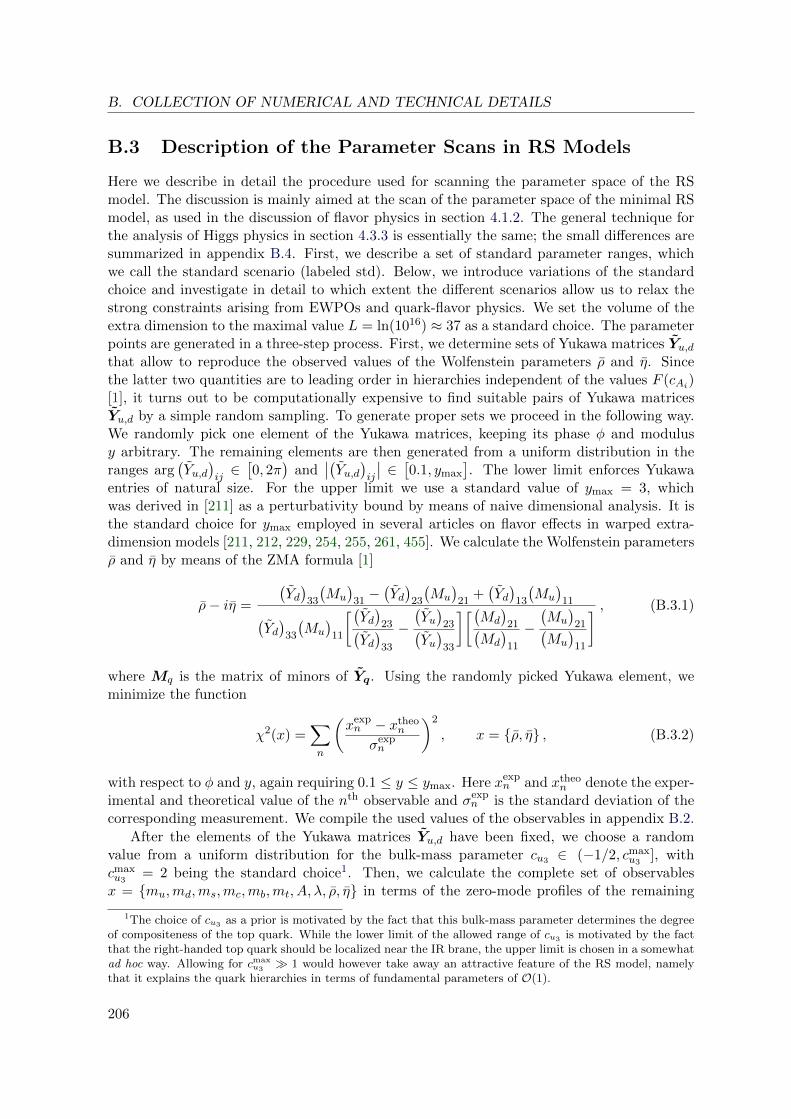
B. COLLECTION OF NUMERICAL AND TECHNICAL DETAILS
B.3 Description of the Parameter Scans in RS Models
Here we describe in detail the procedure used for scanning the parameter space of the RSmodel. The discussion is mainly aimed at the scan of the parameter space of the minimal RSmodel, as used in the discussion of flavor physics in section 4.1.2. The general technique forthe analysis of Higgs physics in section 4.3.3 is essentially the same; the small differences aresummarized in appendix B.4. First, we describe a set of standard parameter ranges, whichwe call the standard scenario (labeled std). Below, we introduce variations of the standardchoice and investigate in detail to which extent the different scenarios allow us to relax thestrong constraints arising from EWPOs and quark-flavor physics. We set the volume of theextra dimension to the maximal value L = ln(1016) ≈ 37 as a standard choice. The parameterpoints are generated in a three-step process. First, we determine sets of Yukawa matrices Yu,dthat allow to reproduce the observed values of the Wolfenstein parameters ρ and η. Sincethe latter two quantities are to leading order in hierarchies independent of the values F (cAi)[1], it turns out to be computationally expensive to find suitable pairs of Yukawa matricesYu,d by a simple random sampling. To generate proper sets we proceed in the following way.We randomly pick one element of the Yukawa matrices, keeping its phase φ and modulusy arbitrary. The remaining elements are then generated from a uniform distribution in theranges arg
(Yu,d
)ij∈[0, 2π
)and
∣∣(Yu,d)ij
∣∣ ∈[0.1, ymax
]. The lower limit enforces Yukawa
entries of natural size. For the upper limit we use a standard value of ymax = 3, whichwas derived in [211] as a perturbativity bound by means of naive dimensional analysis. It isthe standard choice for ymax employed in several articles on flavor effects in warped extra-dimension models [211, 212, 229, 254, 255, 261, 455]. We calculate the Wolfenstein parametersρ and η by means of the ZMA formula [1]
ρ− iη =
(Yd)
33
(Mu
)31−(Yd)
23
(Mu
)21
+(Yd)
13
(Mu
)11
(Yd)
33
(Mu
)11
[(Yd)
23(Yd)
33
−(Yu)
23(Yu)
33
][(Md
)21(
Md
)11
−(Mu
)21(
Mu
)11
] , (B.3.1)
where Mq is the matrix of minors of Yq. Using the randomly picked Yukawa element, weminimize the function
χ2(x) =∑
n
(xexpn − xtheo
n
σexpn
)2
, x = ρ, η , (B.3.2)
with respect to φ and y, again requiring 0.1 ≤ y ≤ ymax. Here xexpn and xtheo
n denote the exper-imental and theoretical value of the nth observable and σexp
n is the standard deviation of thecorresponding measurement. We compile the used values of the observables in appendix B.2.
After the elements of the Yukawa matrices Yu,d have been fixed, we choose a randomvalue from a uniform distribution for the bulk-mass parameter cu3 ∈ (−1/2, cmax
u3], with
cmaxu3
= 2 being the standard choice1. Then, we calculate the complete set of observablesx = mu,md,ms,mc,mb,mt, A, λ, ρ, η in terms of the zero-mode profiles of the remaining
1The choice of cu3 as a prior is motivated by the fact that this bulk-mass parameter determines the degreeof compositeness of the top quark. While the lower limit of the allowed range of cu3 is motivated by the factthat the right-handed top quark should be localized near the IR brane, the upper limit is chosen in a somewhatad hoc way. Allowing for cmax
u3 1 would however take away an attractive feature of the RS model, namely
that it explains the quark hierarchies in terms of fundamental parameters of O(1).
206
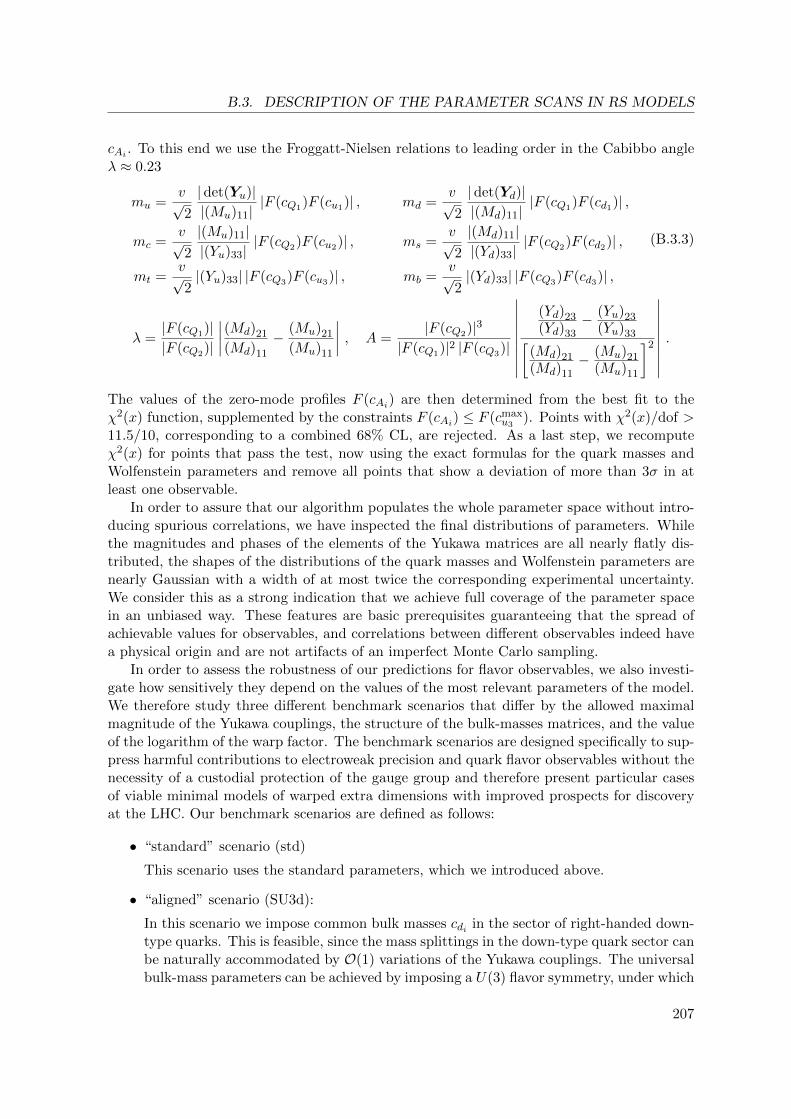
B.3. DESCRIPTION OF THE PARAMETER SCANS IN RS MODELS
cAi . To this end we use the Froggatt-Nielsen relations to leading order in the Cabibbo angleλ ≈ 0.23
mu =v√2
|det(Yu)||(Mu)11|
|F (cQ1)F (cu1)| , md =v√2
| det(Yd)||(Md)11|
|F (cQ1)F (cd1)| ,
mc =v√2
|(Mu)11||(Yu)33|
|F (cQ2)F (cu2)| , ms =v√2
|(Md)11||(Yd)33|
|F (cQ2)F (cd2)| ,
mt =v√2|(Yu)33| |F (cQ3)F (cu3)| , mb =
v√2|(Yd)33| |F (cQ3)F (cd3)| ,
(B.3.3)
λ =|F (cQ1)||F (cQ2)|
∣∣∣∣(Md)21
(Md)11
− (Mu)21
(Mu)11
∣∣∣∣ , A =|F (cQ2)|3
|F (cQ1)|2 |F (cQ3)|
∣∣∣∣∣∣∣∣∣
(Yd)23(Yd)33
− (Yu)23(Yu)33[
(Md)21(Md)11
− (Mu)21(Mu)11
]2
∣∣∣∣∣∣∣∣∣.
The values of the zero-mode profiles F (cAi) are then determined from the best fit to theχ2(x) function, supplemented by the constraints F (cAi) ≤ F (cmax
u3). Points with χ2(x)/dof >
11.5/10, corresponding to a combined 68% CL, are rejected. As a last step, we recomputeχ2(x) for points that pass the test, now using the exact formulas for the quark masses andWolfenstein parameters and remove all points that show a deviation of more than 3σ in atleast one observable.
In order to assure that our algorithm populates the whole parameter space without intro-ducing spurious correlations, we have inspected the final distributions of parameters. Whilethe magnitudes and phases of the elements of the Yukawa matrices are all nearly flatly dis-tributed, the shapes of the distributions of the quark masses and Wolfenstein parameters arenearly Gaussian with a width of at most twice the corresponding experimental uncertainty.We consider this as a strong indication that we achieve full coverage of the parameter spacein an unbiased way. These features are basic prerequisites guaranteeing that the spread ofachievable values for observables, and correlations between different observables indeed havea physical origin and are not artifacts of an imperfect Monte Carlo sampling.
In order to assess the robustness of our predictions for flavor observables, we also investi-gate how sensitively they depend on the values of the most relevant parameters of the model.We therefore study three different benchmark scenarios that differ by the allowed maximalmagnitude of the Yukawa couplings, the structure of the bulk-masses matrices, and the valueof the logarithm of the warp factor. The benchmark scenarios are designed specifically to sup-press harmful contributions to electroweak precision and quark flavor observables without thenecessity of a custodial protection of the gauge group and therefore present particular casesof viable minimal models of warped extra dimensions with improved prospects for discoveryat the LHC. Our benchmark scenarios are defined as follows:
• “standard” scenario (std)
This scenario uses the standard parameters, which we introduced above.
• “aligned” scenario (SU3d):
In this scenario we impose common bulk masses cdi in the sector of right-handed down-type quarks. This is feasible, since the mass splittings in the down-type quark sector canbe naturally accommodated by O(1) variations of the Yukawa couplings. The universalbulk-mass parameters can be achieved by imposing a U(3) flavor symmetry, under which
207

B. COLLECTION OF NUMERICAL AND TECHNICAL DETAILS
standard aligned LRS
cQ1 −0.63± 0.03 −0.66± 0.02 −1.34± 0.16
cQ2 −0.57± 0.05 −0.59± 0.03 −1.04± 0.18
cQ3 −0.34± 0.32 −0.24± 0.43 −0.49± 0.34
cu1 −0.68± 0.04 −0.65± 0.03 −1.58± 0.18
cu2 −0.51± 0.12 −0.50± 0.12 −0.79± 0.26
cu3 ]− 1/2, 2] ]− 1/2, 2] ]− 1/2, 5/2]
cd1 −0.65± 0.03 −0.60± 0.02 −1.44± 0.17
cd2 −0.62± 0.03 −0.60± 0.02 −1.28± 0.17
cd3 −0.58± 0.03 −0.60± 0.02 −1.05± 0.13
Table B.1: Central values and statistical uncertainties of the bulk-mass parameters in thethree benchmark scenarios. The shown errors correspond to 1σ ranges when fitting thedistributions to a Gaussian function, except for cu3
for which a flat prior is chosen in thegiven range. See text for details.
the fields that give rise to the right-handed down-type quark zero modes transformas triplets, and all other fields as singlets [254]. Besides the natural suppression ofcorrections to εK [254], this scenario has the appealing feature that it leads to a uniquepattern of deviations in the K → πνν sector.
• little RS scenario (LRS):
From a purely phenomenological point of view, it is possible to lower the UV cutofffrom the Planck scale to a value only few orders of magnitude above the TeV scale,even though in this case a true solution to the hierarchy problem is postponed to higherenergy. Since many amplitudes in the RS model are enhanced by L, it is worthwhileto address the question to what extent certain experimental constraints can be avoidedby such a choice [192]. Thus, we consider a “volume-truncated” variant of our firstscenario characterized by L = ln(103) ≈ 7. This affects the amount of splitting betweenthe bulk-mass parameters, which is necessary to achieve the fermion hierarchies. Inorder to cover the full shape of the distributions for the bulk-mass parameters, we allowfor cmax
u3= 5/2. In this “little” RS scenario [192] the bound from oblique EWPOs is
lowered to a size that is comparable to the custodial model (see figure 4.12). However, noimprovement concerning εK is achieved compared to the standard benchmark scenario[229].
The statistical approach outlined in the last section provides us with distributions of bulk-mass parameters rather than with their precise values. The obtained results are differentin the individual benchmark scenarios, and in order to make this work self-contained, wesummarize the central values and standard deviations of the parameters cAi for the threecases in table B.1. We also illustrate the distribution in the standard scenario in figure B.1.All distributions are nearly Gaussian, apart from those of cQ3 , which feature a small tail tohigher values, and those of cu3 , which are chosen as flat priors. Notice that while the centralvalues of the bulk-mass parameters in the standard and aligned benchmark scenarios are verysimilar, the splitting between the individual cAi parameters is on average much bigger in the
208

B.3. DESCRIPTION OF THE PARAMETER SCANS IN RS MODELS
-0.8 -0.6 -0.4 -0.2 0.0cQ0.00
0.05
0.10
0.15
0.20
rel . frequency
-0.5 0.0 0.5 1.0 1.5 2.0cu0.00
0.05
0.10
0.15
0.20
0.25
rel . frequency
-0.8 -0.7 -0.6 -0.5cd0.00
0.02
0.04
0.06
0.08
0.10
0.12
rel . frequency
Figure B.1: Bulk-mass parameter distribution resulting from the Monte Carlo sampling withstandard parameter choices (std).
LRS scenario due to the smaller “volume factor” L. We have verified that the precise formof the distributions is essentially independent of the details of the algorithm used to scan theparameter space. Besides inspecting the coverage of our Monte-Carlo sampling, we also assesthe numerical and perturbative stability of each single parameter point. For this purpose weuse the quantitative measure for fine-tuning
∆BG(O) = maxp∈P
∣∣∂ln(p) ln(O)∣∣ , (B.3.4)
introduced by Barbieri and Giudice [326]. In our case, the set of model parameters P includesthe Yukawa couplings, their complex conjugates, and the bulk masses.
We identify two different situations, where ∆BG(O) can become large, rendering the resultsunstable under small variations of the input parameters. The first case corresponds to largevalues of the observable O, where the variation is dominated by a single contribution. In
this case it is sufficient to apply the fine-tuning measure to the matrices ∆(′)A and δA, defined
in (3.3.145) and (3.3.148), which constitute the new-physics contributions to all the relevantcouplings (KK photons and gluons, Z boson and its KK excitations) in our analysis. Inpractice, we use the analytic form of those matrices from [1], obtained from a Froggatt-
Nielsen analysis to leading order in λ. The contributions to ∆BG(∆(′)A , δA) stemming from
variations of the bulk-mass parameters cAi scale either as L or 1 if cAi < −1/2 or cAi > −1/2.Similarly, variations with respect to the Yukawa entries typically lead to contributions of O(1),but can also become larger if individual elements (Yu,d)ij appearing in the denominators of
the expressions for ∆(′)A and δA cancel each other. However, even in such a case the resulting
contribution to ∆BG(∆(′)A , δA) never exceeds 100 for points consistent with the observed quark
masses and mixing, implying no severe fine-tuning.
The situation is different for untypically small values of O. As we show explicitly insection 4.1.2.4, this situation occurs in the case of |εK |, where the experimental constraintforces the new-physics contribution to be small compared to the typical values that arise in themodel at hand. In this case we calculate ∆BG(|εK |) taking into account the full expressionfor |εK | with all interferences and RG effects, and reject parameter points that show anexcessive fine-tuning stronger than one per mil, i.e. ∆BG(|εK |) > 1000. The resulting datasets consist of more than 60, 000 valid parameter points in each scenario. We have verifiedthat (reasonable) variations of the chosen cut on ∆BG(|εK |) neither change the shape of thedistribution of allowed scatter points nor affect any of our conclusions. In contrast, restrictingthe amount of allowed fine-tuning to values of around 10 would result in distributions thatshow a sharp cutoff of values below the lower end of the experimental allowed region of |εK |.
209
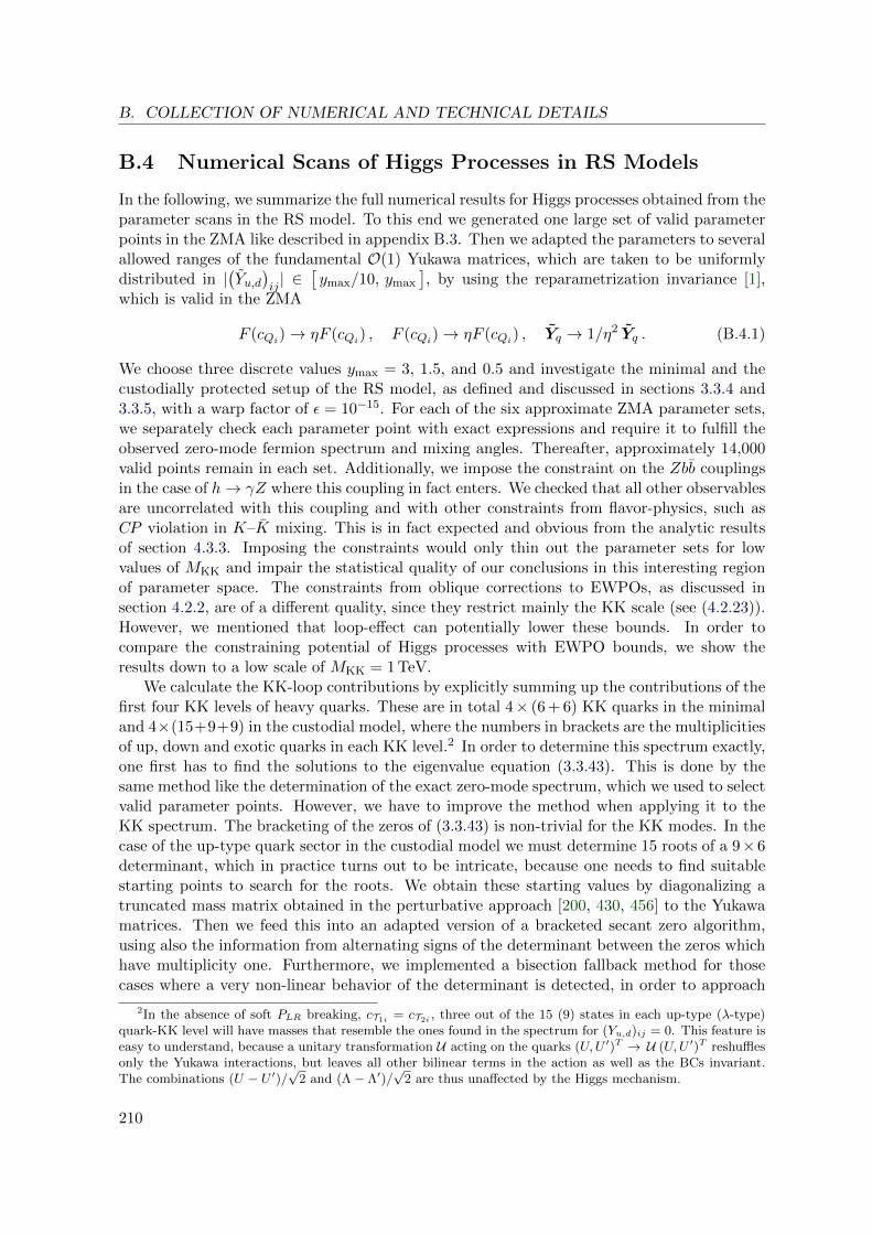
B. COLLECTION OF NUMERICAL AND TECHNICAL DETAILS
B.4 Numerical Scans of Higgs Processes in RS Models
In the following, we summarize the full numerical results for Higgs processes obtained from theparameter scans in the RS model. To this end we generated one large set of valid parameterpoints in the ZMA like described in appendix B.3. Then we adapted the parameters to severalallowed ranges of the fundamental O(1) Yukawa matrices, which are taken to be uniformlydistributed in |
(Yu,d
)ij| ∈
[ymax/10, ymax
], by using the reparametrization invariance [1],
which is valid in the ZMA
F (cQi)→ ηF (cQi) , F (cQi)→ ηF (cQi) , Yq → 1/η2 Yq . (B.4.1)
We choose three discrete values ymax = 3, 1.5, and 0.5 and investigate the minimal and thecustodially protected setup of the RS model, as defined and discussed in sections 3.3.4 and3.3.5, with a warp factor of ε = 10−15. For each of the six approximate ZMA parameter sets,we separately check each parameter point with exact expressions and require it to fulfill theobserved zero-mode fermion spectrum and mixing angles. Thereafter, approximately 14,000valid points remain in each set. Additionally, we impose the constraint on the Zbb couplingsin the case of h→ γZ where this coupling in fact enters. We checked that all other observablesare uncorrelated with this coupling and with other constraints from flavor-physics, such asCP violation in K–K mixing. This is in fact expected and obvious from the analytic resultsof section 4.3.3. Imposing the constraints would only thin out the parameter sets for lowvalues of MKK and impair the statistical quality of our conclusions in this interesting regionof parameter space. The constraints from oblique corrections to EWPOs, as discussed insection 4.2.2, are of a different quality, since they restrict mainly the KK scale (see (4.2.23)).However, we mentioned that loop-effect can potentially lower these bounds. In order tocompare the constraining potential of Higgs processes with EWPO bounds, we show theresults down to a low scale of MKK = 1 TeV.
We calculate the KK-loop contributions by explicitly summing up the contributions of thefirst four KK levels of heavy quarks. These are in total 4× (6 + 6) KK quarks in the minimaland 4×(15+9+9) in the custodial model, where the numbers in brackets are the multiplicitiesof up, down and exotic quarks in each KK level.2 In order to determine this spectrum exactly,one first has to find the solutions to the eigenvalue equation (3.3.43). This is done by thesame method like the determination of the exact zero-mode spectrum, which we used to selectvalid parameter points. However, we have to improve the method when applying it to theKK spectrum. The bracketing of the zeros of (3.3.43) is non-trivial for the KK modes. In thecase of the up-type quark sector in the custodial model we must determine 15 roots of a 9×6determinant, which in practice turns out to be intricate, because one needs to find suitablestarting points to search for the roots. We obtain these starting values by diagonalizing atruncated mass matrix obtained in the perturbative approach [200, 430, 456] to the Yukawamatrices. Then we feed this into an adapted version of a bracketed secant zero algorithm,using also the information from alternating signs of the determinant between the zeros whichhave multiplicity one. Furthermore, we implemented a bisection fallback method for thosecases where a very non-linear behavior of the determinant is detected, in order to approach
2In the absence of soft PLR breaking, cT1i = cT2i , three out of the 15 (9) states in each up-type (λ-type)quark-KK level will have masses that resemble the ones found in the spectrum for (Yu,d)ij = 0. This feature iseasy to understand, because a unitary transformation U acting on the quarks (U,U ′)T → U (U,U ′)T reshufflesonly the Yukawa interactions, but leaves all other bilinear terms in the action as well as the BCs invariant.The combinations (U − U ′)/
√2 and (Λ− Λ′)/
√2 are thus unaffected by the Higgs mechanism.
210
B.4. NUMERICAL SCANS OF HIGGS PROCESSES IN RS MODELS
the zero faster. We implemented this in the computational software program Mathematicawith optimized and parallelized code. This allows to generate the large data sets in roughlyone week of single-core CPU time on modern machines.
Having the numerical result at hand, we can verify the analytic results of section 4.3.3 asan additional check. To achieve a high precision for the numerical results we extrapolate the
sum entering Σ(low)q from the first four KK levels to the resummed result, by using
∞∑
n=1
v gqnnmqn
=v
MKK
( nf+nF∑
n=1
gqnnxqn
+ ρ2,4
nf+4nF∑
n=nf+nF+1
gqnnxqn
). (B.4.2)
The factor ρm,n summarizes the extrapolation of the contribution from all higher KK levels,starting from the (n + 1)th, based on the numerical result for the mth up to the nth level,which have to be found numerically. We choose to exclude the 1st KK level from the extrap-olation. Above that a very regular pattern emerges, such that the factor ρm,n can be derivedanalytically. We make use of the knowledge that the summed contributions from the kth
KK level scale approximately with ∼ (((k − 1)π − xq1)2 − (xq0)2)−1, where we set xq0,1 to theaverage value of the zero mode and first KK-level masses. Numerically this turns out to bevery accurate for approximating the unknown higher KK-level contributions. The resummedcorrection factor is analytically given by
ρm,n =
(1− ψ0(n+ (xq1 + xq0)/π)− ψ0(n+ (xq1 − xq0)/π)
ψ0(m− 1 + (xq1 + xq0)/π)− ψ0(m− 1 + (xq1 − xq0)/π)
)−1
=
(1− ψ′0(n+ xq1/π)
ψ′0(m− 1 + xq1/π)
)−1
+ O(
(xq0)2
6π2
),
(B.4.3)
where ψ0 denotes the digamma function. The extrapolation factor turns out to be independentof xq0 to very good precision, such that we neglect this dependence and use ρ2,4 ≈ 1.209 +0.237
(xq1/2.5
). Remark that this rescales the contributions starting from the second level and
only has a minor impact compared to the contribution from the first KK level. However, itis reassuring for the check of the analytical result and verifying statements about their bulkmass independence.
In the figures B.2–B.10 we show all two-dimensional fits to the parameter distribution ofthe KK scale versus a given cross-section ratio, width ratio, or ratio of branching ratios, whichwe defined in section 4.3.4. The cyan curves correspond to the 5%, 20%, 50%, 80%, and 95%quantiles. Thus, at a given scale MKK, 60% / 90% of the parameter space is contained in thelight / dark blue bands. The bands are underlaid with the parameter points in faint yellow.The fits to the quantiles are obtained by first applying a fine grained binning in x-direction,calculating the quantiles, and then fitting a global model to the resulting distributions. Sincethe observables involve absolute values and interfering amplitudes of different parametricbehavior, we choose in each case a fit model that is adapted to the data and check for ahigh quality of the fit. By default we try to use a quadratic polynomial3 in (TeV/MKK)2. Inthe case of the total Higgs width and ymax = 3, and also for Rγγ/RZZ and ymax = 3 in thecustodial model, it is necessary and sufficient to extend the model to a Pade approximant,i.e. the ratio of two quadratic polynomials. In all other cases, where an extremum arises
3We use three fit parameters, one being the normalization. We check that the normalization turns out tobe like expected, i.e. one in most cases.
211

B. COLLECTION OF NUMERICAL AND TECHNICAL DETAILS
due to the aforementioned reasons, we resort to a more sophisticated model. This involvesthe sum of Fermi-functions, each multiplied by a quadratic polynomial. The Fermi-functionssmoothly connect two regions, where e.g. a sign shift in the amplitude implies a minimumfor the absolute value of the amplitude. This is necessary since the quantile of the resultingdistribution does not exhibit a kink but rather has a smooth minimum.
Remark that, in order to obtain a reliable fit result, we have to exclude the region whereless than 10% of the parameter points survive the bound on the Zbb-couplings from the fit toRγZ . This bound is shown in the left panel of figure 4.16 and discussed in the correspondingsection of the main text.
In the following, we enlist the pseudo-observables in the order in which they are discussedin the main text of section 4.3.4. A discussion of the results is given there.
212
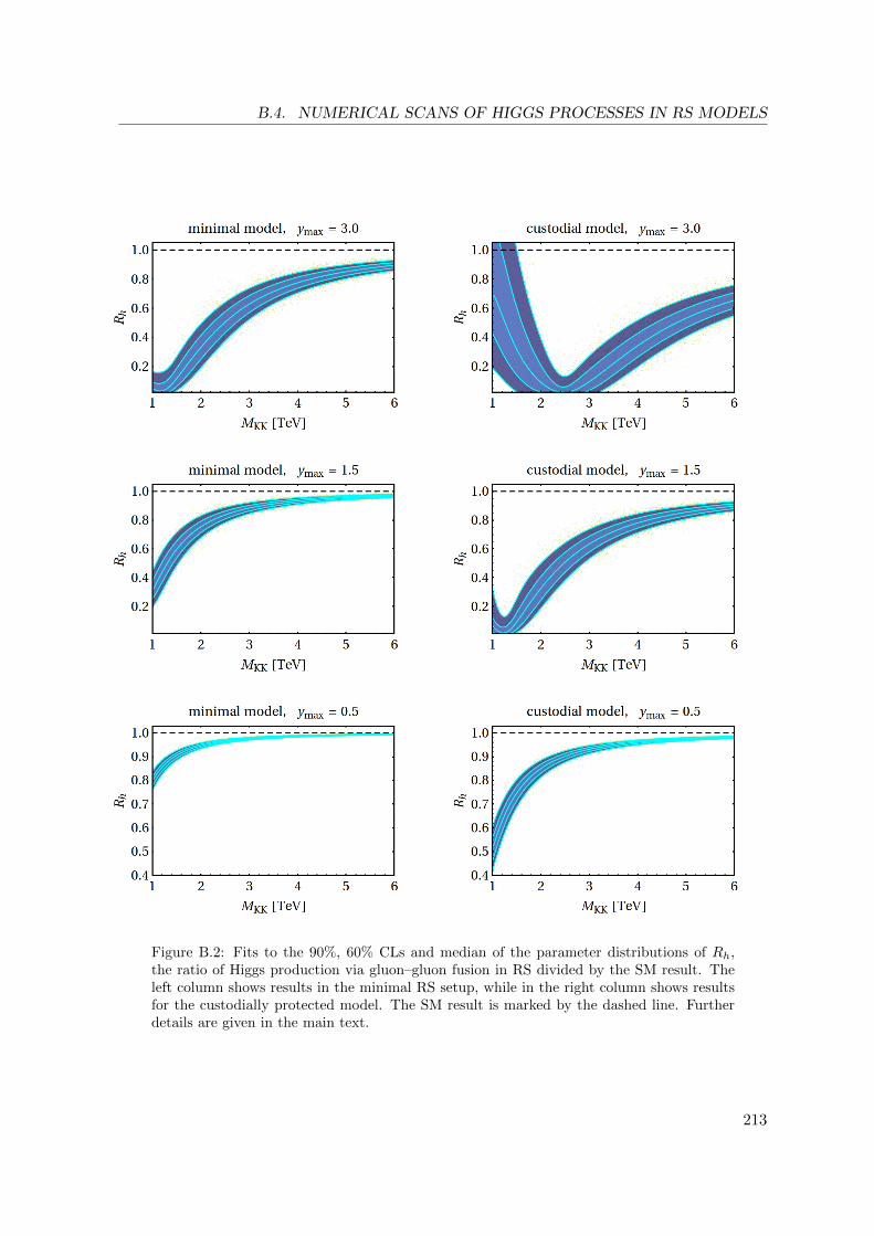
B.4. NUMERICAL SCANS OF HIGGS PROCESSES IN RS MODELS
Figure B.2: Fits to the 90%, 60% CLs and median of the parameter distributions of Rh,the ratio of Higgs production via gluon–gluon fusion in RS divided by the SM result. Theleft column shows results in the minimal RS setup, while in the right column shows resultsfor the custodially protected model. The SM result is marked by the dashed line. Furtherdetails are given in the main text.
213

B. COLLECTION OF NUMERICAL AND TECHNICAL DETAILS
Figure B.3: Fits to the 90%, 60% CLs and median of the parameter distributions of thebranching ratio for h→ bb in the RS model divided by the SM result. The left column showsresults in the minimal RS setup, while in the right column shows results for the custodiallyprotected model. The SM result is marked by the dashed line. Further details are given inthe main text.
214

B.4. NUMERICAL SCANS OF HIGGS PROCESSES IN RS MODELS
Figure B.4: Fits to the 90%, 60% CLs and median of the parameter distributions of thebranching ratio for h → ZZ in the RS model divided by the SM result. The left columnshows results in the minimal RS setup, while in the right column shows results for thecustodially protected model. The SM result is marked by the dashed line. Further detailsare given in the main text.
215

B. COLLECTION OF NUMERICAL AND TECHNICAL DETAILS
Figure B.5: Fits to the 90%, 60% CLs and median of the parameter distributions of RZZ ,the predicted signal strength of the process gg → h → ZZ in the RS model. The leftcolumn shows results in the minimal RS setup, while in the right column shows results forthe custodially protected model. The SM result is marked by the dashed line. Furtherdetails are given in the main text.
216

B.4. NUMERICAL SCANS OF HIGGS PROCESSES IN RS MODELS
Figure B.6: Fits to the 90%, 60% CLs and median of the parameter distributions of RΓ, theratio of the total Higgs width in the RS model divided by the SM result. The left columnshows results in the minimal RS setup, while in the right column shows results for thecustodially protected model. The SM result is marked by the dashed line. Further detailsare given in the main text.
217
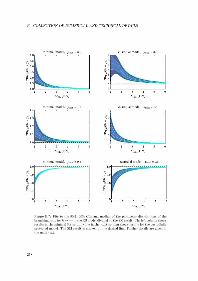
B. COLLECTION OF NUMERICAL AND TECHNICAL DETAILS
Figure B.7: Fits to the 90%, 60% CLs and median of the parameter distributions of thebranching ratio for h→ γγ in the RS model divided by the SM result. The left column showsresults in the minimal RS setup, while in the right column shows results for the custodiallyprotected model. The SM result is marked by the dashed line. Further details are given inthe main text.
218
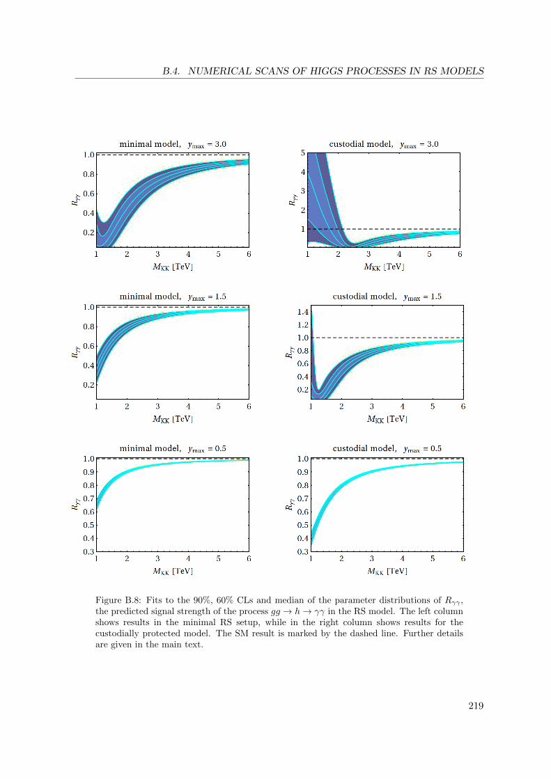
B.4. NUMERICAL SCANS OF HIGGS PROCESSES IN RS MODELS
Figure B.8: Fits to the 90%, 60% CLs and median of the parameter distributions of Rγγ ,the predicted signal strength of the process gg → h→ γγ in the RS model. The left columnshows results in the minimal RS setup, while in the right column shows results for thecustodially protected model. The SM result is marked by the dashed line. Further detailsare given in the main text.
219
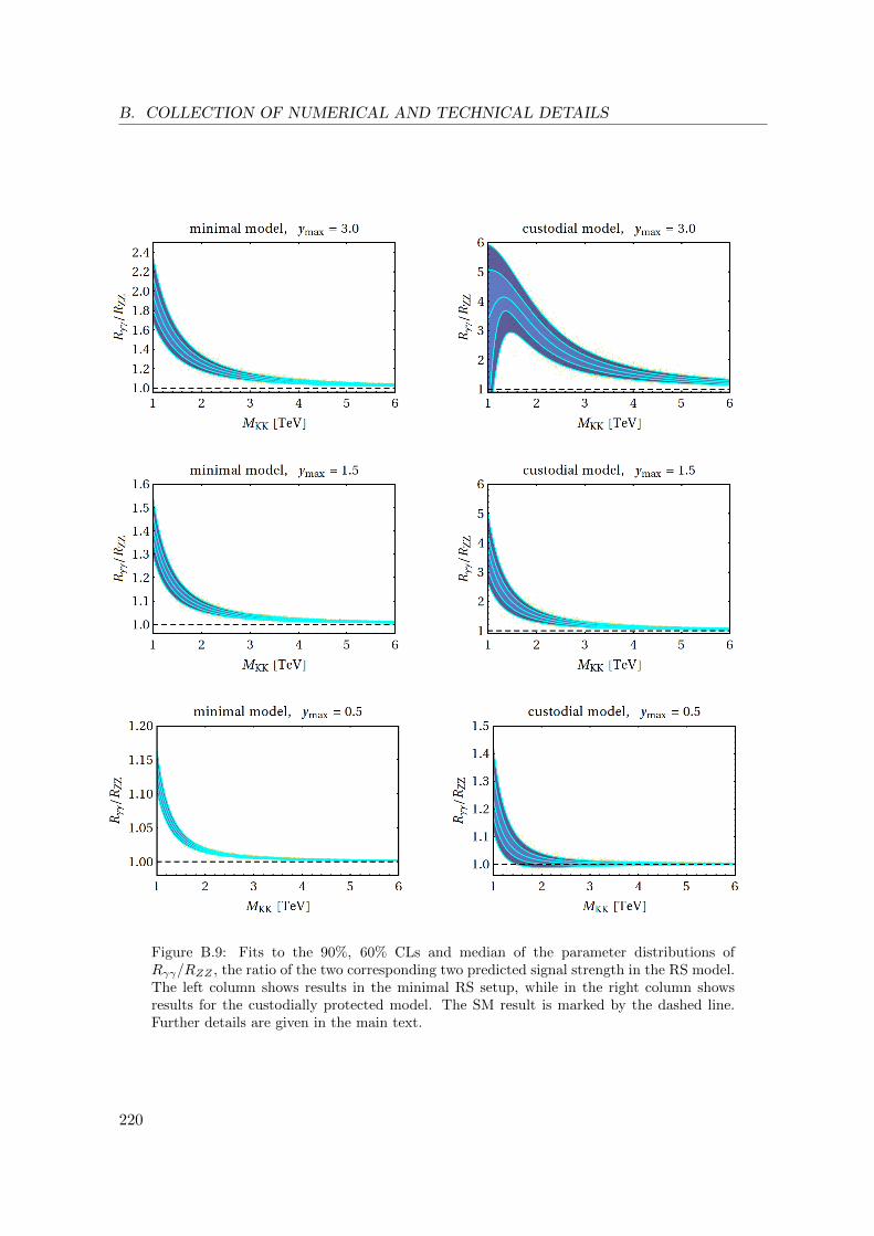
B. COLLECTION OF NUMERICAL AND TECHNICAL DETAILS
Figure B.9: Fits to the 90%, 60% CLs and median of the parameter distributions ofRγγ/RZZ , the ratio of the two corresponding two predicted signal strength in the RS model.The left column shows results in the minimal RS setup, while in the right column showsresults for the custodially protected model. The SM result is marked by the dashed line.Further details are given in the main text.
220

B.4. NUMERICAL SCANS OF HIGGS PROCESSES IN RS MODELS
Figure B.10: Fits to the 90%, 60% CLs and median of the parameter distributions of thebranching ratio for h → γZ in the RS model divided by the SM result. The left columnshows results in the minimal RS setup, while in the right column shows results for thecustodially protected model. The SM result is marked by the dashed line. Further detailsare given in the main text.
221

222

Bibliography
[1] S. Casagrande, F. Goertz, U. Haisch, M. Neubert, and T. Pfoh JHEP 0810 (2008) 094,arXiv:0807.4937.
[2] M. Carena, S. Casagrande, F. Goertz, U. Haisch, and M. Neubert JHEP 1208 (2012) 156,arXiv:1204.0008.
[3] M. Bauer, S. Casagrande, U. Haisch, and M. Neubert JHEP 1009 (2010) 017,arXiv:0912.1625.
[4] S. Casagrande, F. Goertz, U. Haisch, M. Neubert, and T. Pfoh JHEP 1009 (2010) 014,arXiv:1005.4315.
[5] S. Glashow Nucl.Phys. 22 (1961) 579–588.[6] S. Weinberg Phys.Rev.Lett. 19 (1967) 1264–1266.[7] A. Salam Conf.Proc. C680519 (1968) 367–377. Originally printed in *Svartholm: Elementary
Particle Theory, Proceedings Of The Nobel Symposium Held 1968 At Lerum, Sweden*,Stockholm 1968, 367-377.
[8] D. Gross and F. Wilczek Phys.Rev.Lett. 30 (1973) 1343–1346.[9] H. D. Politzer Phys.Rev.Lett. 30 (1973) 1346–1349.
[10] D. Gross and F. Wilczek Phys.Rev. D8 (1973) 3633–3652.[11] M. Gell-Mann Phys.Lett. 8 (1964) 214–215.[12] G. Zweig. In *Lichtenberg, D. B. ( Ed.), Rosen, S. P. ( Ed.): Developments In The Quark
Theory Of Hadrons, Vol. 1*, 22-101 and CERN-TH-401 & CERN-TH-412 (unpublished).[13] J. I. Friedman, H. W. Kendall, and R. E. Taylor Rev. Mod. Phys. 63 (Jul, 1991) 629–629.
http://link.aps.org/doi/10.1103/RevModPhys.63.629.[14] Gargamelle Neutrino Collaboration, F. Hasert et al. Phys.Lett. B46 (1973) 138–140.[15] TASSO Collaboration, R. Brandelik et al. Phys.Lett. B86 (1979) 243.[16] S. Glashow, J. Iliopoulos, and L. Maiani Phys.Rev. D2 (1970) 1285–1292.[17] SLAC-SP-017 Collaboration, J. Augustin et al. Phys.Rev.Lett. 33 (1974) 1406–1408.[18] E598 Collaboration, J. Aubert et al. Phys.Rev.Lett. 33 (1974) 1404–1406.[19] M. Kobayashi and T. Maskawa Prog.Theor.Phys. 49 (1973) 652–657.[20] CDF Collaboration, F. Abe et al. Phys.Rev.Lett. 74 (1995) 2626–2631,
arXiv:hep-ex/9503002.[21] D0 Collaboration, S. Abachi et al. Phys.Rev.Lett. 74 (1995) 2422–2426,
arXiv:hep-ex/9411001.[22] ATLAS Collaboration, G. Aad et al. Phys.Lett.B (2012) , arXiv:1207.7214.[23] ATLAS Collaboration Tech. Rep. ATLAS-CONF-2012-091, Jul, 2012.[24] ATLAS Collaboration Tech. Rep. ATLAS-CONF-2012-127, Sep, 2012.[25] ATLAS Collaboration Tech. Rep. ATLAS-CONF-2012-162, Nov, 2012.[26] ATLAS Collaboration Tech. Rep. ATLAS-CONF-2012-168, Dec, 2012.[27] ATLAS Collaboration Tech. Rep. ATLAS-CONF-2012-169, Dec, 2012.[28] ATLAS Collaboration Tech. Rep. ATLAS-CONF-2012-170, Dec, 2012.[29] CMS Collaboration, S. Chatrchyan et al. Phys.Lett.B (2012) , arXiv:1207.7235.[30] CMS Collaboration Tech. Rep. CMS-PAS-HIG-12-015, Jul, 2012.[31] CMS Collaboration Tech. Rep. CMS-PAS-HIG-12-020, Jul, 2012.[32] CMS Collaboration Tech. Rep. CMS-PAS-HIG-12-041, Nov, 2012.
223

BIBLIOGRAPHY
[33] CMS Collaboration Tech. Rep. CMS-PAS-HIG-12-042, Nov, 2012.[34] CMS Collaboration Tech. Rep. CMS-PAS-HIG-12-043, Nov, 2012.[35] CMS Collaboration Tech. Rep. CMS-PAS-HIG-12-044, Nov, 2012.[36] CMS Collaboration Tech. Rep. CMS-PAS-HIG-12-045, Nov, 2012.[37] F. Englert and R. Brout Phys.Rev.Lett. 13 (1964) 321–323.[38] P. W. Higgs Phys.Lett. 12 (1964) 132–133.[39] P. W. Higgs Phys.Rev.Lett. 13 (1964) 508–509.[40] G. Guralnik, C. Hagen, and T. Kibble Phys.Rev.Lett. 13 (1964) 585–587.[41] CDF Collaboration, D0 Collaboration, T. Aaltonen et al. Phys.Rev.Lett. 109 (2012)
071804, arXiv:1207.6436.[42] CDF Collaboration, D0 Collaboration, CDF, D. Collaborations, the Tevatron
New Physics, and H. Working arXiv:1207.0449.[43] S. Weinberg arXiv:hep-th/9702027.[44] E. Cartan and P. Adam, Sur la structure des groupes de transformations finis et continus.
Nony, 1894.[45] R. Jost Helv.Phys.Acta 30 (1957) 409–416.[46] G. ’t Hooft and M. Veltman Nucl.Phys. B44 (1972) 189–213.[47] K. G. Wilson Phys.Rev. 179 (1969) 1499–1512.[48] S. Weinberg, The quantum theory of fields. Vol. 2: Modern applications. Cambridge University
Press, 1996.[49] J. C. Collins, Renormalization: An Introduction to Renormalization, the Renormalization
Group and the Operator-Product Expansion. Cambridge monographs on mathematical physics.Cambridge University Press, 1984.
[50] S. Weinberg, The Quantum theory of fields. Vol. 1: Foundations. Cambridge University Press,1995.
[51] S. Weinberg Phys.Rev.Lett. 43 (1979) 1566–1570.[52] W. Buchmuller and D. Wyler Nucl.Phys. B268 (1986) 621.[53] B. Grzadkowski, M. Iskrzynski, M. Misiak, and J. Rosiek JHEP 1010 (2010) 085,
arXiv:1008.4884.[54] C. Burges and H. J. Schnitzer Nucl.Phys. B228 (1983) 464.[55] C. Burgess, S. Godfrey, H. Konig, D. London, and I. Maksymyk Phys.Rev. D49 (1994)
6115–6147, arXiv:hep-ph/9312291.[56] F. del Aguila, M. Perez-Victoria, and J. Santiago Phys.Lett. B492 (2000) 98–106,
arXiv:hep-ph/0007160.[57] Z. Han and W. Skiba Phys.Rev. D71 (2005) 075009, arXiv:hep-ph/0412166.[58] V. Cirigliano, J. Jenkins, and M. Gonzalez-Alonso Nucl.Phys. B830 (2010) 95–115,
arXiv:0908.1754.[59] J. Aguilar-Saavedra Nucl.Phys. B843 (2011) 638–672, arXiv:1008.3562.[60] C. Zhang and S. Willenbrock Phys.Rev. D83 (2011) 034006, arXiv:1008.3869.[61] M. Bohm, A. Denner, and H. Joos, Gauge theories of the strong and electroweak interaction.
Vieweg+Teubner Verlag, 2001.[62] S. L. Adler and W. A. Bardeen Phys.Rev. 182 (1969) 1517–1536.[63] W. A. Bardeen Phys.Rev. 184 (1969) 1848–1857.[64] C. Bouchiat, J. Iliopoulos, and P. Meyer Phys.Lett. B38 (1972) 519–523.[65] H. Georgi and S. L. Glashow Phys.Rev. D6 (1972) 429.[66] D. J. Gross and R. Jackiw Phys.Rev. D6 (1972) 477–493.[67] R. Mohapatra and A. Smirnov Ann.Rev.Nucl.Part.Sci. 56 (2006) 569–628,
arXiv:hep-ph/0603118.[68] N. Cabibbo Phys.Rev.Lett. 10 (1963) 531–533.[69] Particle Data Group, J. Beringer et al. Phys.Rev. D86 (2012) 010001.[70] A. Belavin, A. M. Polyakov, A. Schwartz, and Y. Tyupkin Phys.Lett. B59 (1975) 85–87.[71] G. ’t Hooft Phys.Rev.Lett. 37 (1976) 8–11.[72] G. ’t Hooft Phys.Rev. D14 (1976) 3432–3450.
224

BIBLIOGRAPHY
[73] L. Wolfenstein Phys.Rev.Lett. 51 (1983) 1945.[74] B. Pontecorvo Sov.Phys.JETP 6 (1957) 429.[75] B. Pontecorvo Sov.Phys.JETP 26 (1968) 984–988.[76] Z. Maki, M. Nakagawa, and S. Sakata Prog.Theor.Phys. 28 (1962) 870–880.[77] Daya Bay Collaboration, D. M. Webber arXiv:1211.1609.[78] G. Fogli, E. Lisi, A. Marrone, D. Montanino, A. Palazzo, et al. Phys.Rev. D86 (2012) 013012,
arXiv:1205.5254.[79] S. N. Gupta Proc.Phys.Soc. A63 (1950) 681–691.[80] K. Bleuler Helv.Phys.Acta 23 (1950) 567–586.[81] L. Faddeev and V. Popov Phys.Lett. B25 (1967) 29–30.[82] C. Becchi, A. Rouet, and R. Stora Phys.Lett. B52 (1974) 344.[83] C. Becchi, A. Rouet, and R. Stora Annals Phys. 98 (1976) 287–321.[84] I. Tyutin arXiv:0812.0580.[85] N. Nakanishi Prog. Theor. Phys. 35 (1966) .[86] B. Lautrup Mat. Fys. Medd. Dan. Vid. Selsk. 35 (1967) .[87] C. Grosse-Knetter and R. Kogerler Phys.Rev. D48 (1993) 2865–2876, arXiv:hep-ph/9212268.[88] G. Degrassi, S. Di Vita, J. Elias-Miro, J. R. Espinosa, G. F. Giudice, et al. JHEP 1208 (2012)
098, arXiv:1205.6497.[89] W. Grimus, L. Lavoura, and B. Radovcic Phys.Lett. B674 (2009) 117–121, arXiv:0902.2325.[90] G. Hinshaw, D. Larson, E. Komatsu, D. Spergel, C. Bennett, et al. arXiv:1212.5226.[91] G. Bertone, D. Hooper, and J. Silk Phys.Rept. 405 (2005) 279–390, arXiv:hep-ph/0404175.[92] J. L. Feng Ann.Rev.Astron.Astrophys. 48 (2010) 495–545, arXiv:1003.0904.[93] J. Bond, G. Efstathiou, and J. Silk Phys.Rev.Lett. 45 (1980) 1980–1984.[94] G. Jungman, M. Kamionkowski, and K. Griest Phys.Rept. 267 (1996) 195–373,
arXiv:hep-ph/9506380.[95] T. Appelquist, H.-C. Cheng, and B. A. Dobrescu Phys.Rev. D64 (2001) 035002,
arXiv:hep-ph/0012100.[96] A. Sakharov Pisma Zh.Eksp.Teor.Fiz. 5 (1967) 32–35.[97] M. Gavela, P. Hernandez, J. Orloff, O. Pene, and C. Quimbay Nucl.Phys. B430 (1994)
382–426, arXiv:hep-ph/9406289.[98] A. Pilaftsis J.Phys.Conf.Ser. 171 (2009) 012017, arXiv:0904.1182.[99] H. Georgi and S. Glashow Phys.Rev.Lett. 32 (1974) 438–441.
[100] P. Langacker Phys.Rept. 72 (1981) 185.[101] S. Raby.[102] K. R. Dienes, E. Dudas, and T. Gherghetta Phys.Lett. B436 (1998) 55–65,
arXiv:hep-ph/9803466.[103] L. Randall and M. D. Schwartz JHEP 0111 (2001) 003, arXiv:hep-th/0108114.[104] M. Veltman Acta Phys.Polon. B8 (1977) 475.[105] S. P. Martin arXiv:hep-ph/9709356.[106] A. Djouadi Phys.Rept. 459 (2008) 1–241, arXiv:hep-ph/0503173.[107] M. Veltman Acta Phys.Polon. B12 (1981) 437.[108] S. Weinberg Phys.Rev. D13 (1976) 974–996.[109] E. Gildener Phys.Rev. D14 (1976) 1667.[110] S. Weinberg Rev.Mod.Phys. 61 (1989) 1–23.[111] C. Baker, D. Doyle, P. Geltenbort, K. Green, M. van der Grinten, et al. Phys.Rev.Lett. 97
(2006) 131801, arXiv:hep-ex/0602020.[112] R. Jackiw and C. Rebbi Phys.Rev.Lett. 37 (1976) 172–175.[113] C. Llewellyn Smith Phys.Lett. B46 (1973) 233–236.[114] J. M. Cornwall, D. N. Levin, and G. Tiktopoulos Phys.Rev.Lett. 30 (1973) 1268–1270.[115] J. M. Cornwall, D. N. Levin, and G. Tiktopoulos Phys.Rev. D10 (1974) 1145.[116] B. W. Lee, C. Quigg, and H. Thacker Phys.Rev. D16 (1977) 1519.[117] M. S. Chanowitz, M. Furman, and I. Hinchliffe Phys.Lett. B78 (1978) 285.[118] M. S. Chanowitz, M. Furman, and I. Hinchliffe Nucl.Phys. B153 (1979) 402.
225
BIBLIOGRAPHY
[119] H. A. Weldon Phys.Rev. D30 (1984) 1547.[120] P. Langacker and H. A. Weldon Phys.Rev.Lett. 52 (1984) 1377.[121] J. Gunion, H. Haber, and J. Wudka Phys.Rev. D43 (1991) 904–912.[122] K. Babu, J. Julio, and Y. Zhang Nucl.Phys. B858 (2012) 468–487, arXiv:1111.5021.[123] C. Bobeth, M. Misiak, and J. Urban Nucl.Phys. B567 (2000) 153–185,
arXiv:hep-ph/9904413.[124] A. J. Buras and J. Girrbach JHEP 1203 (2012) 052, arXiv:1201.1302.[125] M. S. Chanowitz and M. K. Gaillard Nucl.Phys. B261 (1985) 379.[126] G. Gounaris, R. Kogerler, and H. Neufeld Phys.Rev. D34 (1986) 3257.[127] T. Hahn Comput.Phys.Commun. 140 (2001) 418–431, arXiv:hep-ph/0012260.[128] K. Fujikawa, B. Lee, and A. Sanda Phys.Rev. D6 (1972) 2923–2943.[129] H.-J. He, Y.-P. Kuang, and C.-P. Yuan Phys.Rev. D51 (1995) 6463–6473,
arXiv:hep-ph/9410400.[130] Y.-P. Yao and C. Yuan Phys.Rev. D38 (1988) 2237.[131] A. J. Buras and J. Girrbach JHEP 1202 (2012) 143, arXiv:1201.2563.[132] T. Ohl and C. Schwinn Eur.Phys.J. C30 (2003) 567–582, arXiv:hep-ph/0305334.[133] C. Schwinn arXiv:hep-ph/0307057.[134] T. Hahn and M. Perez-Victoria Comput.Phys.Commun. 118 (1999) 153–165,
arXiv:hep-ph/9807565.[135] M. Jacob and G. Wick Annals Phys. 7 (1959) 404–428.[136] E. Wigner, Gruppentheorie und ihre Anwendung auf die Quantenmechanik der Atomspektren.
Academic Press, 1959.[137] C. Itzykson and J. Zuber.[138] M. Luscher and P. Weisz Phys.Lett. B212 (1988) 472.[139] W. J. Marciano, G. Valencia, and S. Willenbrock Phys.Rev. D40 (1989) 1725.[140] L. Durand, P. N. Maher, and K. Riesselmann Phys.Rev. D48 (1993) 1084–1096,
arXiv:hep-ph/9303234.[141] K. Riesselmann and S. Willenbrock Phys.Rev. D55 (1997) 311–321, arXiv:hep-ph/9608280.[142] A. Djouadi Phys.Rept. 457 (2008) 1–216, arXiv:hep-ph/0503172.[143] N. Cabibbo, L. Maiani, G. Parisi, and R. Petronzio Nucl.Phys. B158 (1979) 295–305.[144] N. Arkani-Hamed, A. G. Cohen, and H. Georgi Phys.Lett. B513 (2001) 232–240,
arXiv:hep-ph/0105239.[145] N. Arkani-Hamed, A. Cohen, E. Katz, and A. Nelson JHEP 0207 (2002) 034,
arXiv:hep-ph/0206021.[146] D. B. Kaplan and H. Georgi Phys.Lett. B136 (1984) 183.[147] D. B. Kaplan, H. Georgi, and S. Dimopoulos Phys.Lett. B136 (1984) 187.[148] M. Schmaltz JHEP 0408 (2004) 056, arXiv:hep-ph/0407143.[149] S. Chang JHEP 0312 (2003) 057, arXiv:hep-ph/0306034.[150] R. Contino, L. Da Rold, and A. Pomarol Phys.Rev. D75 (2007) 055014,
arXiv:hep-ph/0612048.[151] T. Han, H. E. Logan, B. McElrath, and L.-T. Wang Phys.Rev. D67 (2003) 095004,
arXiv:hep-ph/0301040.[152] A. J. Buras, A. Poschenrieder, S. Uhlig, and W. A. Bardeen JHEP 0611 (2006) 062,
arXiv:hep-ph/0607189.[153] C. Csaki, J. Hubisz, G. D. Kribs, P. Meade, and J. Terning Phys.Rev. D67 (2003) 115002,
arXiv:hep-ph/0211124.[154] J. L. Hewett, F. J. Petriello, and T. G. Rizzo JHEP 0310 (2003) 062, arXiv:hep-ph/0211218.[155] M.-C. Chen and S. Dawson Phys.Rev. D70 (2004) 015003, arXiv:hep-ph/0311032.[156] H.-C. Cheng and I. Low JHEP 0309 (2003) 051, arXiv:hep-ph/0308199.[157] J. Hubisz and P. Meade Phys.Rev. D71 (2005) 035016, arXiv:hep-ph/0411264.[158] I. Low JHEP 0410 (2004) 067, arXiv:hep-ph/0409025.[159] H.-C. Cheng and I. Low JHEP 0408 (2004) 061, arXiv:hep-ph/0405243.[160] T. Goto, Y. Okada, and Y. Yamamoto Phys.Lett. B670 (2009) 378–382, arXiv:0809.4753.
226
BIBLIOGRAPHY
[161] B. Grinstein, R. Kelley, and P. Uttayarat JHEP 0909 (2009) 040, arXiv:0904.1622.[162] B. Grinstein, R. Kelley, and P. Uttayarat PoS ICHEP2010 (2010) 392, arXiv:1102.4010.[163] J. Hubisz, S. J. Lee, and G. Paz JHEP 0606 (2006) 041, arXiv:hep-ph/0512169.[164] A. Belyaev, C.-R. Chen, K. Tobe, and C.-P. Yuan Phys.Rev. D74 (2006) 115020,
arXiv:hep-ph/0609179.[165] M. Blanke, A. J. Buras, A. Poschenrieder, S. Recksiegel, C. Tarantino, et al. JHEP 0701
(2007) 066, arXiv:hep-ph/0610298.[166] I. Low and A. Vichi Phys.Rev. D84 (2011) 045019, arXiv:1010.2753.[167] D. Pappadopulo and A. Vichi JHEP 1103 (2011) 072, arXiv:1007.4807.[168] A. Paul, I. I. Bigi, and S. Recksiegel Phys.Rev. D83 (2011) 114006, arXiv:1101.6053.[169] J. Hubisz, P. Meade, A. Noble, and M. Perelstein JHEP 0601 (2006) 135,
arXiv:hep-ph/0506042.[170] M. Antonelli, D. M. Asner, D. A. Bauer, T. G. Becher, M. Beneke, et al. Phys.Rept. 494
(2010) 197–414, arXiv:0907.5386.[171] F. del Aguila, J. Illana, and M. Jenkins JHEP 1009 (2010) 040, arXiv:1006.5914.[172] S. R. Coleman, J. Wess, and B. Zumino Phys.Rev. 177 (1969) 2239–2247.[173] J. Callan, Curtis G., S. R. Coleman, J. Wess, and B. Zumino Phys.Rev. 177 (1969) 2247–2250.[174] M. Blanke, A. J. Buras, A. Poschenrieder, S. Recksiegel, C. Tarantino, et al. Phys.Lett. B646
(2007) 253–257, arXiv:hep-ph/0609284.[175] L. Randall and R. Sundrum Phys.Rev.Lett. 83 (1999) 3370–3373, arXiv:hep-ph/9905221.[176] N. Arkani-Hamed, S. Dimopoulos, and G. Dvali Phys.Lett. B429 (1998) 263–272,
arXiv:hep-ph/9803315.[177] D. Kapner, T. Cook, E. Adelberger, J. Gundlach, B. R. Heckel, et al. Phys.Rev.Lett. 98 (2007)
021101, arXiv:hep-ph/0611184.[178] S. Cullen and M. Perelstein Phys.Rev.Lett. 83 (1999) 268–271, arXiv:hep-ph/9903422.[179] V. Rubakov and M. Shaposhnikov Phys.Lett. B125 (1983) 136–138.[180] N. Arkani-Hamed and M. Schmaltz Phys.Rev. D61 (2000) 033005, arXiv:hep-ph/9903417.[181] I. R. Klebanov and M. J. Strassler JHEP 0008 (2000) 052, arXiv:hep-th/0007191.[182] S. B. Giddings, S. Kachru, and J. Polchinski Phys.Rev. D66 (2002) 106006,
arXiv:hep-th/0105097.[183] S. Kachru, R. Kallosh, A. D. Linde, and S. P. Trivedi Phys.Rev. D68 (2003) 046005,
arXiv:hep-th/0301240.[184] F. Brummer, A. Hebecker, and E. Trincherini Nucl.Phys. B738 (2006) 283–305,
arXiv:hep-th/0510113.[185] H. Davoudiasl, J. Hewett, and T. Rizzo Phys.Lett. B473 (2000) 43–49,
arXiv:hep-ph/9911262.[186] Y. Grossman and M. Neubert Phys.Lett. B474 (2000) 361–371, arXiv:hep-ph/9912408.[187] C. Csaki, J. Erlich, and J. Terning Phys.Rev. D66 (2002) 064021, arXiv:hep-ph/0203034.[188] W. D. Goldberger and M. B. Wise Phys.Rev.Lett. 83 (1999) 4922–4925,
arXiv:hep-ph/9907447.[189] J. Hewett and T. Rizzo JHEP 0308 (2003) 028, arXiv:hep-ph/0202155.[190] C. Csaki, J. Hubisz, and S. J. Lee Phys.Rev. D76 (2007) 125015, arXiv:0705.3844.[191] H. de Sandes and R. Rosenfeld Phys.Rev. D85 (2012) 053003, arXiv:1111.2006.[192] H. Davoudiasl, G. Perez, and A. Soni Phys.Lett. B665 (2008) 67–71, arXiv:0802.0203.[193] A. Pomarol Phys.Lett. B486 (2000) 153–157, arXiv:hep-ph/9911294.[194] S. Chang, J. Hisano, H. Nakano, N. Okada, and M. Yamaguchi Phys.Rev. D62 (2000) 084025,
arXiv:hep-ph/9912498.[195] T. Gherghetta and A. Pomarol Nucl.Phys. B586 (2000) 141–162, arXiv:hep-ph/0003129.[196] S. J. Huber and Q. Shafi Phys.Rev. D63 (2001) 045010, arXiv:hep-ph/0005286.[197] H. Davoudiasl, J. Hewett, and T. Rizzo Phys.Rev. D63 (2001) 075004,
arXiv:hep-ph/0006041.[198] S. J. Huber, C.-A. Lee, and Q. Shafi Phys.Lett. B531 (2002) 112–118, arXiv:hep-ph/0111465.[199] S. J. Huber and Q. Shafi Phys.Lett. B498 (2001) 256–262, arXiv:hep-ph/0010195.
227

BIBLIOGRAPHY
[200] S. J. Huber Nucl.Phys. B666 (2003) 269–288, arXiv:hep-ph/0303183.[201] K. Agashe, G. Perez, and A. Soni Phys.Rev.Lett. 93 (2004) 201804, arXiv:hep-ph/0406101.[202] K. Agashe, G. Perez, and A. Soni Phys.Rev. D71 (2005) 016002, arXiv:hep-ph/0408134.[203] J. Scherk and J. H. Schwarz Phys.Lett. B82 (1979) 60.[204] L. Nilse arXiv:hep-ph/0601015.[205] E. Stueckelberg Helv.Phys.Acta 11 (1938) 225–244.[206] A. Pais Journal of Mathematical Physics 3 no. 6, (1962) 1135–1139.[207] A. Azatov, M. Toharia, and L. Zhu Phys.Rev. D80 (2009) 035016, arXiv:0906.1990.[208] R. Bertlmann, Anomalies in quantum field theory, vol. 91 of International Series of
Monographs on Physics. Oxford University Press, 1996.[209] C. Csaki, J. Hubisz, and P. Meade arXiv:hep-ph/0510275.[210] F. Goertz arXiv:1112.6387.[211] C. Csaki, A. Falkowski, and A. Weiler JHEP 0809 (2008) 008, arXiv:0804.1954.[212] M. Blanke, A. J. Buras, B. Duling, S. Gori, and A. Weiler JHEP 0903 (2009) 001,
arXiv:0809.1073.[213] J. A. Bagger, F. Feruglio, and F. Zwirner Phys.Rev.Lett. 88 (2002) 101601,
arXiv:hep-th/0107128.[214] K. Agashe, A. Delgado, M. J. May, and R. Sundrum JHEP 0308 (2003) 050,
arXiv:hep-ph/0308036.[215] C. Csaki, C. Grojean, L. Pilo, and J. Terning Phys.Rev.Lett. 92 (2004) 101802,
arXiv:hep-ph/0308038.[216] K. Agashe, R. Contino, L. Da Rold, and A. Pomarol Phys.Lett. B641 (2006) 62–66,
arXiv:hep-ph/0605341.[217] H. Georgi, E. E. Jenkins, and E. H. Simmons Phys.Rev.Lett. 62 (1989) 2789. [Erratum-ibid.
63, 1540 (1989)].[218] H. Georgi, E. E. Jenkins, and E. H. Simmons Nucl.Phys. B331 (1990) 541.[219] V. D. Barger, E. Ma, and K. Whisnant Phys.Rev.Lett. 46 (1981) 1501.[220] X. Li and E. Ma Phys.Rev.Lett. 47 (1981) 1788.[221] E. Malkawi, T. M. Tait, and C. Yuan Phys.Lett. B385 (1996) 304–310,
arXiv:hep-ph/9603349.[222] G. Isidori PoS CD09 (2009) 073, arXiv:0911.3219.[223] G. Burdman and L. Da Rold JHEP 0811 (2008) 025, arXiv:0809.4009.[224] M. S. Carena, E. Ponton, J. Santiago, and C. E. Wagner Nucl.Phys. B759 (2006) 202–227,
arXiv:hep-ph/0607106.[225] M. E. Albrecht, M. Blanke, A. J. Buras, B. Duling, and K. Gemmler JHEP 0909 (2009) 064,
arXiv:0903.2415.[226] S. Casagrande diploma thesis, Johannes-Gutenberg Universitat Mainz.
http://wwwthep.physik.uni-mainz.de/Publications/theses/dip-casagrande.pdf.[227] C. Froggatt and H. B. Nielsen Nucl.Phys. B147 (1979) 277.[228] T. Appelquist and J. Carazzone Phys.Rev. D11 (1975) 2856.[229] M. Bauer, S. Casagrande, L. Grunder, U. Haisch, and M. Neubert Phys.Rev. D79 (2009)
076001, arXiv:0811.3678.[230] C. Csaki, Y. Grossman, P. Tanedo, and Y. Tsai Phys.Rev. D83 (2011) 073002,
arXiv:1004.2037.[231] M. Beneke, P. Dey, and J. Rohrwild arXiv:1209.5897.[232] M. Blanke, B. Shakya, P. Tanedo, and Y. Tsai JHEP 1208 (2012) 038, arXiv:1203.6650.[233] M. S. Carena, A. Delgado, E. Ponton, T. M. Tait, and C. Wagner Phys.Rev. D71 (2005)
015010, arXiv:hep-ph/0410344.[234] J. Hirn and V. Sanz Phys.Rev. D76 (2007) 044022, arXiv:hep-ph/0702005.[235] M. Puchwein and Z. Kunszt Annals Phys. 311 (2004) 288–313, arXiv:hep-th/0309069.[236] A. Falkowski Phys.Rev. D77 (2008) 055018, arXiv:0711.0828.[237] I. Low, R. Rattazzi, and A. Vichi JHEP 1004 (2010) 126, arXiv:0907.5413.[238] K. Agashe and R. Contino Phys.Rev. D80 (2009) 075016, arXiv:0906.1542.
228

BIBLIOGRAPHY
[239] A. J. Buras, B. Duling, and S. Gori JHEP 0909 (2009) 076, arXiv:0905.2318.[240] N. D. Christensen and C. Duhr Comput.Phys.Commun. 180 (2009) 1614–1641,
arXiv:0806.4194.[241] B. Grinstein, M. Redi, and G. Villadoro JHEP 1011 (2010) 067, arXiv:1009.2049.[242] T. Feldmann JHEP 1104 (2011) 043, arXiv:1010.2116.[243] F. del Aguila, M. Perez-Victoria, and J. Santiago JHEP 0009 (2000) 011,
arXiv:hep-ph/0007316.[244] A. J. Buras, C. Grojean, S. Pokorski, and R. Ziegler JHEP 1108 (2011) 028,
arXiv:1105.3725.[245] A. J. Buras, P. H. Chankowski, J. Rosiek, and L. Slawianowska Nucl.Phys. B659 (2003) 3,
arXiv:hep-ph/0210145.[246] P. Gambino, P. Grassi, and F. Madricardo Phys.Lett. B454 (1999) 98–104,
arXiv:hep-ph/9811470.[247] A. Denner and T. Sack Nucl. Phys. B347 (1990) 203–216.[248] A. J. Buras arXiv:hep-ph/9806471. To appear in ’Probing the Standard Model of Particle
Interactions’, F.David and R. Gupta, eds., 1998, Elsevier Science B.V.[249] C. Nishi Am.J.Phys. 73 (2005) 1160–1163, arXiv:hep-ph/0412245.[250] M. Gorbahn, S. Jager, U. Nierste, and S. Trine Phys.Rev. D84 (2011) 034030,
arXiv:0901.2065.[251] T. Inami and C. Lim Prog.Theor.Phys. 65 (1981) 297.[252] B. Yang, X. Wang, and J. Han Nucl.Phys. B847 (2011) 1–16, arXiv:1103.2506.[253] M. Blanke, A. J. Buras, A. Poschenrieder, C. Tarantino, S. Uhlig, et al. JHEP 0612 (2006)
003, arXiv:hep-ph/0605214.[254] J. Santiago JHEP 0812 (2008) 046, arXiv:0806.1230.[255] K. Agashe, A. Azatov, and L. Zhu Phys.Rev. D79 (2009) 056006, arXiv:0810.1016.[256] S. J. Huber and Q. Shafi Phys.Lett. B544 (2002) 295–306, arXiv:hep-ph/0205327.[257] S. J. Huber and Q. Shafi Phys.Lett. B583 (2004) 293–303, arXiv:hep-ph/0309252.[258] K. Agashe, T. Okui, and R. Sundrum Phys.Rev.Lett. 102 (2009) 101801, arXiv:0810.1277.[259] M. Carena, A. D. Medina, N. R. Shah, and C. E. Wagner Phys.Rev. D79 (2009) 096010,
arXiv:0901.0609.[260] LHCb Collaboration, R. Aaij et al. arXiv:1211.2674.[261] M. Blanke, A. J. Buras, B. Duling, K. Gemmler, and S. Gori JHEP 0903 (2009) 108,
arXiv:0812.3803.[262] R. Kitano Phys.Lett. B481 (2000) 39–44, arXiv:hep-ph/0002279.[263] W.-F. Chang and J. N. Ng Phys.Rev. D71 (2005) 053003, arXiv:hep-ph/0501161.[264] K. Agashe, A. E. Blechman, and F. Petriello Phys.Rev. D74 (2006) 053011,
arXiv:hep-ph/0606021.[265] G. Perez and L. Randall JHEP 0901 (2009) 077, arXiv:0805.4652.[266] B. Lillie, L. Randall, and L.-T. Wang JHEP 0709 (2007) 074, arXiv:hep-ph/0701166.[267] K. Agashe, A. Belyaev, T. Krupovnickas, G. Perez, and J. Virzi Phys.Rev. D77 (2008) 015003,
arXiv:hep-ph/0612015.[268] ATLAS Collaboration, G. Aad et al. arXiv:1211.2202.[269] CMS Collaboration, S. Chatrchyan et al. JHEP 1212 (2012) 015, arXiv:1209.4397.[270] J. A. Bagger, K. T. Matchev, and R.-J. Zhang Phys.Lett. B412 (1997) 77–85,
arXiv:hep-ph/9707225.[271] M. Ciuchini, V. Lubicz, L. Conti, A. Vladikas, A. Donini, et al. JHEP 9810 (1998) 008,
arXiv:hep-ph/9808328.[272] A. J. Buras, M. Misiak, and J. Urban Nucl.Phys. B586 (2000) 397–426,
arXiv:hep-ph/0005183.[273] B. Duling JHEP 1005 (2010) 109, arXiv:0912.4208.[274] V. Bertone, N. Carrasco, M. Ciuchini, P. Dimopoulos, R. Frezzotti, et al. arXiv:1207.1287.[275] A. J. Buras, D. Guadagnoli, and G. Isidori Phys.Lett. B688 (2010) 309–313, arXiv:1002.3612.[276] K. Anikeev, D. Atwood, F. Azfar, S. Bailey, C. Bauer, et al. arXiv:hep-ph/0201071.
229
BIBLIOGRAPHY
[277] E. Andriyash, G. Ovanesyan, and M. Vysotsky Phys.Lett. B599 (2004) 253–259,arXiv:hep-ph/0310314.
[278] E. Andriyash, G. Ovanesyan, and M. Vysotsky Phys.Atom.Nucl. 69 (2006) 286–292,arXiv:hep-ph/0502111.
[279] J. Brod and M. Gorbahn Phys.Rev.Lett. 108 (2012) 121801, arXiv:1108.2036.[280] G. Beall, M. Bander, and A. Soni Phys.Rev.Lett. 48 (1982) 848.[281] F. Gabbiani, E. Gabrielli, A. Masiero, and L. Silvestrini Nucl.Phys. B477 (1996) 321–352,
arXiv:hep-ph/9604387.[282] G. Colangelo, J. Gasser, and H. Leutwyler Nucl.Phys. B603 (2001) 125–179,
arXiv:hep-ph/0103088.[283] A. J. Buras, M. Jamin, and M. E. Lautenbacher Nucl.Phys. B408 (1993) 209–285,
arXiv:hep-ph/9303284.[284] S. Bosch, A. Buras, M. Gorbahn, S. Jager, M. Jamin, et al. Nucl.Phys. B565 (2000) 3–37,
arXiv:hep-ph/9904408.[285] A. J. Buras, M. Jamin, M. Lautenbacher, and P. H. Weisz Nucl.Phys. B370 (1992) 69–104.[286] A. J. Buras, M. Jamin, M. E. Lautenbacher, and P. H. Weisz Nucl.Phys. B400 (1993) 37–74,
arXiv:hep-ph/9211304.[287] A. J. Buras, M. Jamin, and M. E. Lautenbacher Nucl.Phys. B400 (1993) 75–102,
arXiv:hep-ph/9211321.[288] M. Ciuchini, E. Franco, G. Martinelli, and L. Reina Phys.Lett. B301 (1993) 263–271,
arXiv:hep-ph/9212203.[289] M. Ciuchini, E. Franco, G. Martinelli, and L. Reina Nucl.Phys. B415 (1994) 403–462,
arXiv:hep-ph/9304257.[290] P. Gambino and U. Haisch JHEP 0009 (2000) 001, arXiv:hep-ph/0007259.[291] A. J. Buras and M. Jamin JHEP 0401 (2004) 048, arXiv:hep-ph/0306217.[292] J. Bijnens and J. Prades Nucl.Phys.Proc.Suppl. 96 (2001) 354–363, arXiv:hep-ph/0010008.[293] J. Bijnens, E. Gamiz, and J. Prades JHEP 0110 (2001) 009, arXiv:hep-ph/0108240.[294] M. Knecht, S. Peris, and E. de Rafael Phys.Lett. B508 (2001) 117–126,
arXiv:hep-ph/0102017.[295] T. Hambye, S. Peris, and E. de Rafael JHEP 0305 (2003) 027, arXiv:hep-ph/0305104.[296] RBC Collaboration, T. Blum et al. Phys.Rev. D68 (2003) 114506, arXiv:hep-lat/0110075.[297] P. Boucaud, V. Gimenez, C. D. Lin, V. Lubicz, G. Martinelli, et al. Nucl.Phys. B721 (2005)
175–211, arXiv:hep-lat/0412029.[298] T. Bhattacharya, N. Christ, G. T. Fleming, G. Kilcup, R. Gupta, et al. Nucl.Phys.Proc.Suppl.
106 (2002) 311–313, arXiv:hep-lat/0111004.[299] T. Bhattacharya, G. T. Fleming, R. Gupta, G. Kilcup, W. Lee, et al. Nucl.Phys.Proc.Suppl.
140 (2005) 369–371, arXiv:hep-lat/0409046.[300] P. Boyle, N. Christ, N. Garron, E. Goode, T. Janowski, et al. arXiv:1212.1474.[301] E. Pallante, A. Pich, and I. Scimemi Nucl.Phys. B617 (2001) 441–474,
arXiv:hep-ph/0105011.[302] F. Mescia and C. Smith Phys.Rev. D76 (2007) 034017, arXiv:0705.2025.[303] G. Buchalla and A. J. Buras Nucl.Phys. B548 (1999) 309–327, arXiv:hep-ph/9901288.[304] M. Misiak and J. Urban Phys.Lett. B451 (1999) 161–169, arXiv:hep-ph/9901278.[305] J. Brod, M. Gorbahn, and E. Stamou Phys.Rev. D83 (2011) 034030, arXiv:1009.0947.[306] G. Isidori, F. Mescia, and C. Smith Nucl.Phys. B718 (2005) 319–338, arXiv:hep-ph/0503107.[307] A. Buras, M. Gorbahn, U. Haisch, and U. Nierste Phys.Rev.Lett. 95 (2005) 261805,
arXiv:hep-ph/0508165.[308] A. J. Buras, M. Gorbahn, U. Haisch, and U. Nierste JHEP 0611 (2006) 002,
arXiv:hep-ph/0603079.[309] J. Brod and M. Gorbahn Phys.Rev. D78 (2008) 034006, arXiv:0805.4119.[310] F. Mescia, C. Smith, and S. Trine JHEP 0608 (2006) 088, arXiv:hep-ph/0606081.[311] M. Gorbahn and U. Haisch Phys.Rev.Lett. 97 (2006) 122002, arXiv:hep-ph/0605203.[312] G. Isidori and R. Unterdorfer JHEP 0401 (2004) 009, arXiv:hep-ph/0311084.
230

BIBLIOGRAPHY
[313] J.-M. Gerard, C. Smith, and S. Trine Nucl.Phys. B730 (2005) 1–36, arXiv:hep-ph/0508189.[314] A. J. Buras, M. E. Lautenbacher, M. Misiak, and M. Munz Nucl.Phys. B423 (1994) 349–383,
arXiv:hep-ph/9402347.[315] NA48/1 Collaboration, J. Batley et al. Phys.Lett. B576 (2003) 43–54,
arXiv:hep-ex/0309075.[316] NA48/1 Collaboration, J. Batley et al. Phys.Lett. B599 (2004) 197–211,
arXiv:hep-ex/0409011.[317] G. Buchalla, G. D’Ambrosio, and G. Isidori Nucl.Phys. B672 (2003) 387–408,
arXiv:hep-ph/0308008.[318] S. Friot, D. Greynat, and E. De Rafael Phys.Lett. B595 (2004) 301–308,
arXiv:hep-ph/0404136.[319] K. De Bruyn, R. Fleischer, R. Knegjens, P. Koppenburg, M. Merk, et al. Phys.Rev.Lett. 109
(2012) 041801, arXiv:1204.1737.[320] S. Jager and J. M. Camalich arXiv:1212.2263.[321] A. J. Buras, J. Girrbach, D. Guadagnoli, and G. Isidori Eur.Phys.J. C72 (2012) 2172,
arXiv:1208.0934.[322] C. Cheung, A. L. Fitzpatrick, and L. Randall JHEP 0801 (2008) 069, arXiv:0711.4421.[323] Heavy Flavor Averaging Group, Y. Amhis et al. arXiv:1207.1158.[324] ATLAS Collaboration tech. rep., 1999.[325] CMS Collaboration, G. Bayatian et al. J.Phys. G34 (2007) 995–1579.[326] R. Barbieri and G. Giudice Nucl.Phys. B306 (1988) 63.[327] A. J. Buras, M. Jamin, and P. H. Weisz Nucl.Phys. B347 (1990) 491–536.[328] E949 Collaboration, A. Artamonov et al. Phys.Rev.Lett. 101 (2008) 191802,
arXiv:0808.2459.[329] E391a Collaboration, J. Ahn et al. Phys.Rev. D81 (2010) 072004, arXiv:0911.4789.[330] Y. Grossman and Y. Nir Phys.Lett. B398 (1997) 163–168, arXiv:hep-ph/9701313.[331] M. Blanke Acta Phys.Polon. B41 (2010) 127, arXiv:0904.2528.[332] A. J. Buras Phys.Lett. B566 (2003) 115–119, arXiv:hep-ph/0303060.[333] A. Buras, P. Gambino, M. Gorbahn, S. Jager, and L. Silvestrini Phys.Lett. B500 (2001)
161–167, arXiv:hep-ph/0007085.[334] S. Davidson, G. Isidori, and S. Uhlig Phys.Lett. B663 (2008) 73–79, arXiv:0711.3376.[335] O. Gedalia, G. Isidori, and G. Perez Phys.Lett. B682 (2009) 200–206, arXiv:0905.3264.[336] R. Bouchendira, P. Clade, S. Guellati-Khelifa, F. Nez, and F. Biraben Physical Review Letters
106 no. 8, (Feb., 2011) 080801, arXiv:1012.3627.[337] J. Erler and P. Langacker.[338] ALEPH Collaboration, DELPHI Collaboration, L3 Collaboration, OPAL
Collaboration, SLD Collaboration, LEP Electroweak Working Group, SLDElectroweak Group, SLD Heavy Flavour Group, S. Schael et al. Phys.Rept. 427 (2006)257–454, arXiv:hep-ex/0509008.
[339] SLD Collaboration, K. Abe et al. Phys.Rev.Lett. 84 (2000) 5945–5949,arXiv:hep-ex/0004026.
[340] CMS Collaboration, S. Chatrchyan et al. Phys.Rev. D84 (2011) 112002, arXiv:1110.2682.[341] D. Y. Bardin, P. Christova, M. Jack, L. Kalinovskaya, A. Olchevski, et al.
Comput.Phys.Commun. 133 (2001) 229–395, arXiv:hep-ph/9908433.A. Arbuzov, M. Awramik, M. Czakon, A. Freitas, M. Grunewald, et al.Comput.Phys.Commun. 174 (2006) 728–758, arXiv:hep-ph/0507146.
[342] J. Erler arXiv:hep-ph/0005084.[343] H. Flacher, M. Goebel, J. Haller, A. Hocker, K. Monig, et al. Eur.Phys.J. C60 (2009) 543–583,
arXiv:0811.0009.M. Baak, M. Goebel, J. Haller, A. Hoecker, D. Ludwig, et al. Eur.Phys.J. C72 (2012) 2003,arXiv:1107.0975.
[344] M. Baak, M. Goebel, J. Haller, A. Hoecker, D. Kennedy, et al. arXiv:1209.2716.[345] A. Freitas and Y.-C. Huang JHEP 1208 (2012) 050, arXiv:1205.0299.
231

BIBLIOGRAPHY
[346] S. Heinemeyer, W. Hollik, and G. Weiglein Phys.Rept. 425 (2006) 265–368,arXiv:hep-ph/0412214.
[347] G. Altarelli and R. Barbieri Phys.Lett. B253 (1991) 161–167.[348] M. E. Peskin and T. Takeuchi Phys.Rev.Lett. 65 (1990) 964–967.[349] M. E. Peskin and T. Takeuchi Phys.Rev. D46 (1992) 381–409.[350] R. Barbieri, A. Pomarol, R. Rattazzi, and A. Strumia Nucl.Phys. B703 (2004) 127–146,
arXiv:hep-ph/0405040.[351] LEP Collaborations, ALEPH Collaboration, DELPHI Collaboration, L3
Collaboration, LEP Electroweak Working Group, SLD Electroweak Group, SLDHeavy Flavour Group, OPAL Collaboration, t. S. Electroweak arXiv:hep-ex/0412015.
[352] R. S. Chivukula, E. H. Simmons, H.-J. He, M. Kurachi, and M. Tanabashi Phys.Lett. B603(2004) 210–218, arXiv:hep-ph/0408262.
[353] M. E. Peskin and J. D. Wells Phys.Rev. D64 (2001) 093003, arXiv:hep-ph/0101342.[354] J. Field Mod.Phys.Lett. A13 (1998) 1937–1954, arXiv:hep-ph/9801355.[355] B. Batell, S. Gori, and L.-T. Wang arXiv:1209.6382.[356] C. Bouchart and G. Moreau Phys.Rev. D80 (2009) 095022, arXiv:0909.4812.[357] M. S. Carena, E. Ponton, T. M. Tait, and C. Wagner Phys.Rev. D67 (2003) 096006,
arXiv:hep-ph/0212307.[358] A. Delgado and A. Falkowski JHEP 0705 (2007) 097, arXiv:hep-ph/0702234.[359] H. Davoudiasl, S. Gopalakrishna, E. Ponton, and J. Santiago New J.Phys. 12 (2010) 075011,
arXiv:0908.1968.[360] M. S. Carena, E. Ponton, J. Santiago, and C. Wagner Phys.Rev. D76 (2007) 035006,
arXiv:hep-ph/0701055.[361] H. Davoudiasl, J. Hewett, and T. Rizzo Phys.Rev. D68 (2003) 045002,
arXiv:hep-ph/0212279.[362] M. S. Carena, A. Delgado, E. Ponton, T. M. Tait, and C. Wagner Phys.Rev. D68 (2003)
035010, arXiv:hep-ph/0305188.[363] H. Georgi, A. K. Grant, and G. Hailu Phys.Lett. B506 (2001) 207–214,
arXiv:hep-ph/0012379.[364] H.-C. Cheng, K. T. Matchev, and M. Schmaltz Phys.Rev. D66 (2002) 036005,
arXiv:hep-ph/0204342.[365] J. A. Cabrer, G. von Gersdorff, and M. Quiros Phys.Lett. B697 (2011) 208–214,
arXiv:1011.2205.[366] A. Carmona, E. Ponton, and J. Santiago JHEP 1110 (2011) 137, arXiv:1107.1500.[367] A. Djouadi, G. Moreau, and F. Richard Nucl.Phys. B773 (2007) 43–64,
arXiv:hep-ph/0610173.[368] C. Bouchart and G. Moreau Nucl.Phys. B810 (2009) 66–96, arXiv:0807.4461.[369] J. F. Gunion, H. E. Haber, G. L. Kane, and S. Dawson Front.Phys. 80 (2000) 1–448.[370] J. F. Gunion arXiv:hep-ph/0212150.[371] L. Landau Dokl.Akad.Nauk Ser.Fiz. 60 (1948) 207–209.[372] C.-N. Yang Phys.Rev. 77 (1950) 242–245.[373] A. Denner Fortsch.Phys. 41 (1993) 307–420, arXiv:0709.1075.[374] G. Passarino and M. Veltman Nucl.Phys. B160 (1979) 151.[375] H. Georgi, S. Glashow, M. Machacek, and D. V. Nanopoulos Phys.Rev.Lett. 40 (1978) 692.[376] A. Djouadi arXiv:1208.3436.[377] T. Plehn Lect.Notes Phys. 844 (2012) 1–193, arXiv:0910.4182.[378] J. R. Ellis, M. K. Gaillard, and D. V. Nanopoulos Nucl.Phys. B106 (1976) 292.[379] M. A. Shifman, A. Vainshtein, M. Voloshin, and V. I. Zakharov Sov.J.Nucl.Phys. 30 (1979)
711–716.[380] B. A. Kniehl and M. Spira Z.Phys. C69 (1995) 77–88, arXiv:hep-ph/9505225.[381] R. V. Harlander, H. Mantler, S. Marzani, and K. J. Ozeren Eur.Phys.J. C66 (2010) 359–372,
arXiv:0912.2104.[382] D. Graudenz, M. Spira, and P. Zerwas Phys.Rev.Lett. 70 (1993) 1372–1375.
232

BIBLIOGRAPHY
[383] M. Spira, A. Djouadi, D. Graudenz, and P. Zerwas Nucl.Phys. B453 (1995) 17–82,arXiv:hep-ph/9504378.
[384] M. Spira arXiv:hep-ph/9510347.[385] R. V. Harlander and W. B. Kilgore Phys.Rev.Lett. 88 (2002) 201801, arXiv:hep-ph/0201206.[386] C. Anastasiou and K. Melnikov Nucl.Phys. B646 (2002) 220–256, arXiv:hep-ph/0207004.[387] V. Ravindran, J. Smith, and W. L. van Neerven Nucl.Phys. B665 (2003) 325–366,
arXiv:hep-ph/0302135.[388] LHC Higgs Cross Section Working Group, S. Dittmaier et al. arXiv:1101.0593.[389] S. Dittmaier, S. Dittmaier, C. Mariotti, G. Passarino, R. Tanaka, et al. arXiv:1201.3084.[390] V. Ahrens, T. Becher, M. Neubert, and L. L. Yang Eur.Phys.J. C62 (2009) 333–353,
arXiv:0809.4283.[391] S. Moch and A. Vogt Phys.Lett. B631 (2005) 48–57, arXiv:hep-ph/0508265.[392] E. Laenen and L. Magnea Phys.Lett. B632 (2006) 270–276, arXiv:hep-ph/0508284.[393] A. Idilbi, X.-d. Ji, J.-P. Ma, and F. Yuan Phys.Rev. D73 (2006) 077501,
arXiv:hep-ph/0509294.[394] V. Ravindran Nucl.Phys. B752 (2006) 173–196, arXiv:hep-ph/0603041.[395] A. Idilbi, X.-d. Ji, and F. Yuan Nucl.Phys. B753 (2006) 42–68, arXiv:hep-ph/0605068.[396] V. Ahrens, T. Becher, M. Neubert, and L. L. Yang Phys.Rev. D79 (2009) 033013,
arXiv:0808.3008.[397] A. Martin, W. Stirling, R. Thorne, and G. Watt Phys.Lett. B652 (2007) 292–299,
arXiv:0706.0459.[398] S. Glashow, D. V. Nanopoulos, and A. Yildiz Phys.Rev. D18 (1978) 1724–1727.[399] D. Jones and S. Petcov Phys.Lett. B84 (1979) 440.[400] R. Cahn and S. Dawson Phys.Lett. B136 (1984) 196.[401] U. Aglietti, A. Belyaev, S. Berge, A. Blum, R. Bonciani, et al. arXiv:hep-ph/0612172.
TeV4LHC Higgs Working Group, http://maltoni.home.cern.ch/maltoni/TeV4LHC/.[402] R. N. Cahn, S. D. Ellis, R. Kleiss, and W. J. Stirling Phys.Rev. D35 (1987) 1626.[403] R. Raitio and W. W. Wada Phys.Rev. D19 (1979) 941.[404] Z. Kunszt Nucl.Phys. B247 (1984) 339.[405] R. M. Barnett, H. E. Haber, and D. E. Soper Nucl.Phys. B306 (1988) 697.[406] D. A. Dicus and S. Willenbrock Phys.Rev. D39 (1989) 751.[407] LEP Working Group for Higgs boson searches, ALEPH Collaboration, DELPHI
Collaboration, L3 Collaboration, OPAL Collaboration, R. Barate et al. Phys.Lett.B565 (2003) 61–75, arXiv:hep-ex/0306033.
[408] TEVNPH (Tevatron New Phenomina and Higgs Working Group), CDF and D0Collaboration arXiv:1107.5518.
[409] ATLAS Collaboration, G. Aad et al. Phys.Rev. D86 (2012) 032003, arXiv:1207.0319.[410] CMS Collaboration, S. Chatrchyan et al. Phys.Lett. B710 (2012) 26–48, arXiv:1202.1488.[411] J. M. Butterworth, A. R. Davison, M. Rubin, and G. P. Salam Phys.Rev.Lett. 100 (2008)
242001, arXiv:0802.2470.[412] A. Djouadi, J. Kalinowski, and M. Spira Comput.Phys.Commun. 108 (1998) 56–74,
arXiv:hep-ph/9704448.[413] H.-Q. Zheng and D.-D. Wu Phys.Rev. D42 (1990) 3760–3763.[414] S. Actis, G. Passarino, C. Sturm, and S. Uccirati Phys.Lett. B670 (2008) 12–17,
arXiv:0809.1301.[415] J. Baglio and A. Djouadi JHEP 1103 (2011) 055, arXiv:1012.0530.[416] G. Belanger, B. Dumont, U. Ellwanger, J. Gunion, and S. Kraml arXiv:1212.5244.[417] Y. Grossman, Z. Surujon, and J. Zupan arXiv:1301.0328.[418] CMS Collaboration, S. Chatrchyan et al. JHEP 1205 (2012) 123, arXiv:1204.1088.[419] ATLAS Collaboration, G. Aad et al. arXiv:1210.5468.[420] G. D. Kribs, T. Plehn, M. Spannowsky, and T. M. Tait Phys.Rev. D76 (2007) 075016,
arXiv:0706.3718.[421] M. S. Chanowitz arXiv:1212.3209.
233

BIBLIOGRAPHY
[422] O. Eberhardt, G. Herbert, H. Lacker, A. Lenz, A. Menzel, et al. arXiv:1209.1101.[423] A. Denner, S. Dittmaier, A. Muck, G. Passarino, M. Spira, et al. Eur.Phys.J. C72 (2012) 1992,
arXiv:1111.6395.[424] G. Giudice, C. Grojean, A. Pomarol, and R. Rattazzi JHEP 0706 (2007) 045,
arXiv:hep-ph/0703164.[425] C.-R. Chen, K. Tobe, and C.-P. Yuan Phys.Lett. B640 (2006) 263–271,
arXiv:hep-ph/0602211.[426] K. Agashe, R. Contino, and A. Pomarol Nucl.Phys. B719 (2005) 165–187,
arXiv:hep-ph/0412089.[427] J. Reuter and M. Tonini arXiv:1212.5930.[428] N. Arkani-Hamed, A. Cohen, E. Katz, A. Nelson, T. Gregoire, et al. JHEP 0208 (2002) 021,
arXiv:hep-ph/0206020.[429] A. Azatov, M. Toharia, and L. Zhu Phys.Rev. D82 (2010) 056004, arXiv:1006.5939.[430] F. Goertz and T. Pfoh JHEP 0810 (2008) 035, arXiv:0809.1378.[431] T. Inami, T. Kubota, and Y. Okada Z.Phys. C18 (1983) 69.[432] A. V. Manohar and M. B. Wise Phys.Lett. B636 (2006) 107–113, arXiv:hep-ph/0601212.[433] C. Delaunay, J. F. Kamenik, G. Perez, and L. Randall arXiv:1207.0474.[434] A. Pomarol Phys.Rev.Lett. 85 (2000) 4004–4007, arXiv:hep-ph/0005293.[435] K.-w. Choi, H. D. Kim, and I.-W. Kim JHEP 0211 (2002) 033, arXiv:hep-ph/0202257.[436] W. D. Goldberger and I. Z. Rothstein Phys.Rev.Lett. 89 (2002) 131601,
arXiv:hep-th/0204160.[437] K. Agashe, A. Delgado, and R. Sundrum Nucl.Phys. B643 (2002) 172–186,
arXiv:hep-ph/0206099.[438] F. J. Petriello JHEP 0205 (2002) 003, arXiv:hep-ph/0204067.[439] G. Cacciapaglia, A. Deandrea, and J. Llodra-Perez JHEP 0906 (2009) 054, arXiv:0901.0927.[440] A. Djouadi and G. Moreau Phys.Lett. B660 (2008) 67–71, arXiv:0707.3800.[441] G. von Gersdorff, M. Quiros, and M. Wiechers arXiv:1208.4300.[442] F. Goertz, U. Haisch, and M. Neubert Phys.Lett. B713 (2012) 23–28, arXiv:1112.5099.[443] C. F. Berger, C. Marcantonini, I. W. Stewart, F. J. Tackmann, and W. J. Waalewijn JHEP
1104 (2011) 092, arXiv:1012.4480.[444] M. Abramowitz and I. A. Stegun, Handbook of Mathematical Functions with Formulas,
Graphs, and Mathematical Tables. Dover, New York, ninth dover printing, tenth gpoprinting ed., Jun, 1964. http://www.math.sfu.ca/~cbm/aands/.
[445] M. Beneke and M. Neubert Nucl.Phys. B651 (2003) 225–248, arXiv:hep-ph/0210085.[446] L. Bergstrom and G. Hulth Nucl.Phys. B259 (1985) 137.[447] CDF Collaboration, D0 Collaboration, T. Aaltonen et al. arXiv:1207.1069.[448] M. Davier, A. Hoecker, B. Malaescu, and Z. Zhang Eur.Phys.J. C71 (2011) 1515,
arXiv:1010.4180.[449] J. Laiho, E. Lunghi, and R. S. Van de Water Phys.Rev. D81 (2010) 034503, arXiv:0910.2928.
Updates available on http://latticeaverages.org/.[450] K. Chetyrkin, J. Kuhn, A. Maier, P. Maierhofer, P. Marquard, et al. Phys.Rev. D80 (2009)
074010, arXiv:0907.2110.[451] J. Brod and M. Gorbahn Phys.Rev. D82 (2010) 094026, arXiv:1007.0684.[452] Heavy Flavor Averaging Group, E. Barberio et al. arXiv:0808.1297.[453] Particle Data Group, C. Amsler et al. Phys.Lett. B667 (2008) 1–1340.[454] CKMfitter Group, J. Charles et al. Eur.Phys.J. C41 (2005) 1–131, arXiv:hep-ph/0406184.[455] C. Csaki, A. Falkowski, and A. Weiler Phys.Rev. D80 (2009) 016001, arXiv:0806.3757.[456] F. del Aguila and J. Santiago Phys.Lett. B493 (2000) 175–181, arXiv:hep-ph/0008143.
234

AcknowledgmentsAnd now for something completely different.
Monty Python
First and foremost I would like to thank my supervisor Martin Gorbahn for the possibilityto work on a enthralling project, the very good collaboration, and for supporting my vagueideas and the help in turning them into a firm work. I would also like to thank him forcomments and suggestions on a first version of this manuscript.
I highly acknowledge the support of Sebastian Jaeger and Matthias Neubert and I wantto thank them for invitations to Sussex and Mainz. The great time in China with Matthiaswill stay lively in my mind.
I want to thank all my other collaborators during the last years Joachim Brod, MartinBauer, Uli Haisch, Florian Goertz, and Torsten Pfoh for their great work and the manyinsights this provided for me.
Lots of small errors have crept into this manuscript in the course of its creation. Thanksto proof-reading from Christoph Bobeth, Joachim Brod, Emmanuel Stamou, Stefan Vickers,Daniel Bolinger, Julia Dietrichs, and Dan Greenwald, many, if not essentially all, were tracedand removed. I like to thank them for straightening some of the most clumsy passages andimproving the readability of the text. I also like to thank the former four of them for beinggreat floor mates, for the many coffee breaks and an open ear for all sorts of things.
A lot of inspiration and knowledge about quantum field theory is thanks to Anna Brunnbauerand David Nolde, who showed great interest in my tutorial on advanced QFT and always hadbrilliant comments.
There are many more people, who have contributed to my work through discussions,questions, comments, and lectures. Please feel acknowledged, even you do not find your namein a list of many here.
I would like to express my gratitude to all the administration and coordination of theExcellence Cluster Universe, for creating excellent working condition, a pleasant atmosphere,and for the well-deserved success in the approval of the cluster continuation.
Many thanks also go to Christoph Promberger and Florian Kuchler for our organiza-tion of the fantastic PhD meeting 2010 Berchtesgaden, and to Thorsten Feldmann for theorganization of the lively and interesting B-physics Workshop in Neckarzimmern.
Personally I profited most from my private environment, my parents, my brother, all ofmy friends, and I deeply thank them for their unconditional support of any kind, the interestin my work, and for keeping me grounded. Most deeply, I thank you Julia for you love andfor your patience.
I gratefully acknowledge the support of the DFG Cluster of Excellence “Origin and Struc-ture of the Universe”.
235