Policy Research Working Paper 5591

Impacts of International Migration and Remittances on Child Outcomes

and Labor Supply in Indonesia

How Does Gender Matter?

Trang NguyenRirin Purnamasari

The World BankEast Asia and Pacific RegionPoverty Reduction and Economic Management UnitMarch 2011

WPS5591P

ublic

Dis

clos

ure

Aut

horiz

edP

ublic

Dis

clos

ure

Aut

horiz

edP

ublic

Dis

clos

ure

Aut

horiz

edP

ublic

Dis

clos

ure

Aut

horiz

ed

Produced by the Research Support Team

Abstract

The Policy Research Working Paper Series disseminates the findings of work in progress to encourage the exchange of ideas about development issues. An objective of the series is to get the findings out quickly, even if the presentations are less than fully polished. The papers carry the names of the authors and should be cited accordingly. The findings, interpretations, and conclusions expressed in this paper are entirely those of the authors. They do not necessarily represent the views of the International Bank for Reconstruction and Development/World Bank and its affiliated organizations, or those of the Executive Directors of the World Bank or the governments they represent.

Policy Research Working Paper 5591

This paper aims to investigate empirically how international migration and remittances in Indonesia, particularly female migration, affect child outcomes and labor supply behavior in sending households. The authors analyze the Indonesia Family Life Survey data set and apply an instrumental variable estimation method, using historical migration networks as instruments for migration and remittance receipts. The study finds that, in Indonesia, the impacts of international migration on sending households are likely to vary depending on the

This paper is a product of the Poverty Reduction and Economic Management Unit, East Asia and Pacific Region. It is part of a larger effort by the World Bank to provide open access to its research and make a contribution to development policy discussions around the world. Policy Research Working Papers are also posted on the Web at http://econ.worldbank.org. The author may be contacted at TNguyen16@worldbank.org.

gender of the migrants. On average, migration reduces the working hours of remaining household members, but this effect is not observed in households with female migrants. At the same time, female migration and their remittances tend to reduce child labor. The estimated impacts of migration and remittances on school enrollment are not statistically significant, but this result is interesting in that the directions of the effects can be opposite when the migrant is male or female

Impacts of International Migration and

Remittances on Child Outcomes and Labor

Supply in Indonesia: How Does Gender Matter?

Trang Nguyen*

Ririn Purnamasari**

.

*East Asia and Pacific Region, The World Bank. Email: TNguyen16@worldbank.org

**East Asia and Pacific Region, The World Bank. Email: rpurnamasari@worldbank.org

We thank Ahmad Ahsan, Richard Adams Jr., Daniel Mont, and participants at the June 2010 conference on

―Cross-Border Labor Mobility‖ in Singapore for their very helpful comments and feedback. We are

grateful to Survey Meter in Indonesia for constructing the IFLS panel data and for providing data support.

Kalpana Mehra and Aaron Szott provided great research assistance. The opinions expressed here are those

of the authors and do not necessarily represent the view of the World Bank, its Executive Directors, or the

countries they represent.

2

1. Introduction

The number of international migrants has been increasing over time. In parallel with

that, the participation of women in international labor migration has also been rising. In

2005, the share of female migrants in the world’s migrant stock was close to half (World

Bank 2008a). Following an upward, global trend in international migration, Indonesia is

now one of the largest migrant labor exporting countries in the world. International

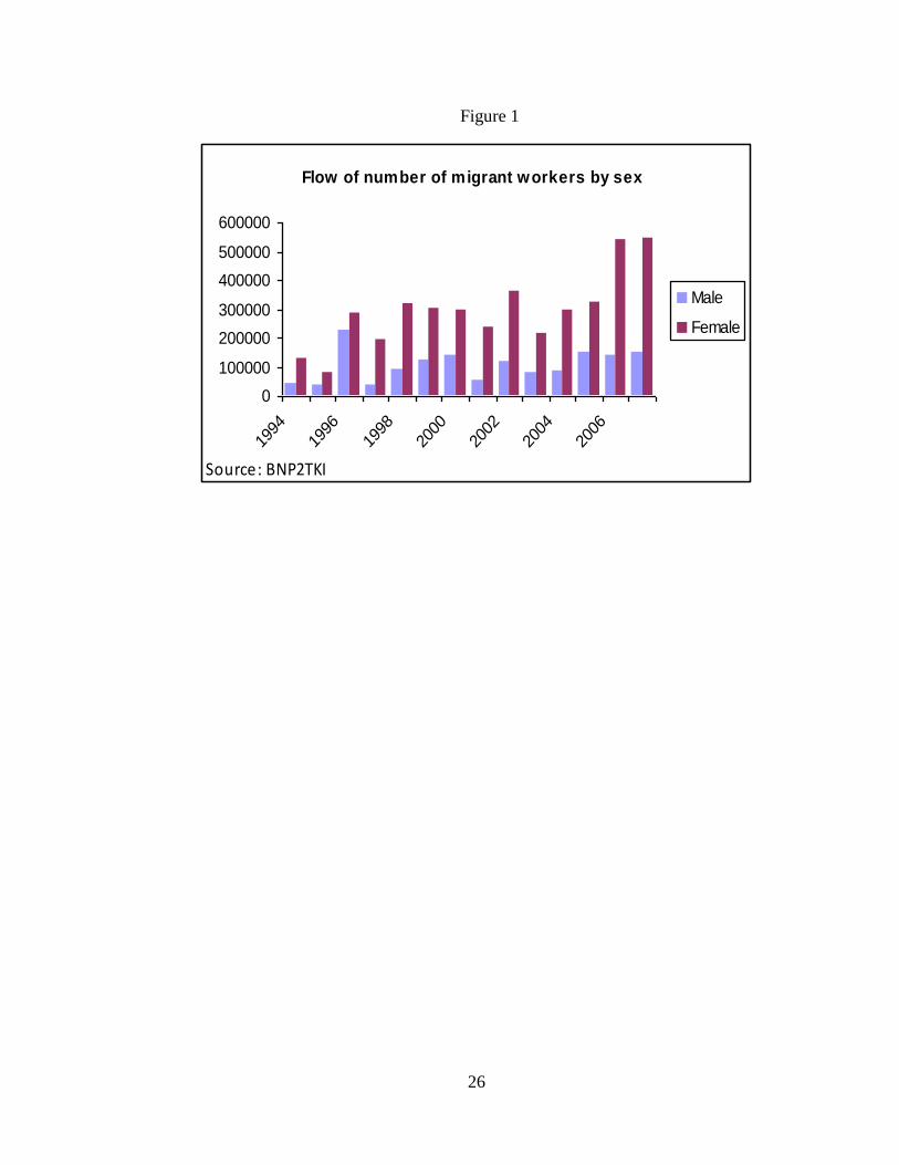
migration from Indonesia has been strongly dominated by women. According to official

records, the number of documented female migrant workers accounted for approximately

80 percent of Indonesia’s migrant workers in 2007 (Figure 1).

The rise in migration has also contributed to the increase in global remittance flows.

Recorded remittances sent home to developing countries were nearly US$ 222 billion in

2006. About 17 percent of global remittances flow back to the East Asia and Pacific

region, including Indonesia. According to the IMF Balance of Payments data, remittances

to Indonesia totaled approximately US$5.7 billion in 2006 (World Bank, 2008b).

Although the amount of remittances appears small relative to total GDP (US$364.5

billion), these inflows may be quite significant in the specific regions of the migrants’

origin.

While international migrant work has become an increasingly important part of the

Indonesian economy, not much research has been done to understand to what extent

migration and remittances may affect the livelihoods of the migrant’s origin household.

The impacts on adult and child labor supply as well as human capital accumulation can

manifest through the income effects of remittances, the impacts on work incentives,

exposure to new information, and consequences of family disconnects. Previous

literature has shown evidence of impacts on the above outcomes in various developing

countries (Adams 2010), though the gender dimension of the impacts has been less

explored. The existing research on international migration from Indonesia mostly

focuses on issues related to the financial literacy and vulnerability of migrant workers.

Such research to date is largely based on qualitative assessments and anecdotal evidence

rather than rigorous quantitative analysis.

This paper fills the gap by quantitatively investigating the development impact of

international migration and remittances in Indonesia, particularly how the migrant’s

3

gender matters. Female migration is of interest since its influence on labor supply and

child outcomes at home might be very different from that of male migration. World

Bank (2008a) argues that men and women show important differences in the

determinants of their decision to migrate as well as their opportunity cost of migration.

Furthermore, the report finds gender differences in the patterns of remittances, budget

allocation of remittance income, and hence gender differences in the impact of migration

or remittances on household decisions and welfare.

Predictions from economic theory regarding the differential impact by the migrant’s

gender on household decisions and outcomes, such as labor supply and education

investment, are ambiguous. With migration and remittances, shifts in income sources

may affect intra-household decision making, which suggests potential gender dimensions

in the impacts on human capital decisions. When a woman moves abroad to work,

increased income from remittances of a female migrant may increase her bargaining

power and her influence over investment choices in the household. However, the

physical absence from the household is expected to create disconnects and loss of control

over the decisions and activities at home. Family disruption can have negative

consequences for children’s welfare, and whether the mother or the father goes away may

matter. Since the net impact is a priori ambiguous, it becomes an important empirical

question.

This study empirically estimates how female and male migration and remittances in

Indonesia affect sending households’ child outcomes and labor supply behavior.1 The

analysis uses nationally representative data of the Indonesia Family Life Survey (IFLS)

2000 and 2007. Estimating the causal impact of migration and remittances is usually

challenging since the decision to migrate and to remit is likely to be endogenous. To

account for endogeneity, this study applies an instrumental variable method using

historical migration networks as instruments for migration and remittance receipts.2

1 The impact on poverty is explored in a parallel paper. Adams and Cuecuecha (2010) find that receiving

remittances reduces the probability of an Indonesian household being poor by 27.8 percent. Other possible

socio-economic effects of migration, such as social impacts, macroeconomic impacts and transfer of

knowledge and skills, are beyond the scope of this paper. 2 McKenzie and Sasin (2007) provide a detailed discussion on the empirical challenges of estimating the

causal impact of migration and possible instruments that have been used in various research questions.

Other papers that have used migration networks as instruments to estimate the impact on outcomes in the

4

Being the first quantitative research, based on a large survey data, in this topic in

Indonesia, this study contributes to a broader view and understanding of the potential

gains and losses from migration for sending households. It also contributes to the limited

existing research on the gender dimensions associated with these gains and losses.

Our results suggest important gender differences in the impacts of international

migration on sending households. In Indonesia, migration reduces the working hours of

remaining household members, but this effect is mainly driven by what happens in

households with male migrants. This negative relationship was not observed for

households with female migrants. The results about child outcomes are also divided

along the gender line. Female migration and their remittances tend to reduce child labor

outside the home but not necessarily boost schooling activities. Though not borne out

statistically significant, the direction of the estimates suggest that migration may have a

slightly positive impact on school enrollment among households with male migrants, but

this impact disappears among those with female migrants. The lack of oversight

associated with the mother’s absence is likely to make it difficult to ensure sufficient

schooling activities for children at home.

The following section reviews the relevant literature. Section 3 describes the IFLS

data, and Section 4 provides a descriptive examination of migrants and migrant-sending

households in Indonesia. The empirical strategy and results are presented in the

subsequent two sections. The last section concludes.

2. Literature Review

While there has not been any quantitative analysis, before this paper, about the

development impacts of migration with a gender focus in the Indonesia context, there is a

general literature on different country experiences of impacts of migration3 and some

indicative evidence on the differential impact by gender. Most studies find that migration

and remittances tend to reduce the labor supply and participation of non-migrating family

home country include Hildebrandt and McKenzie (2005), Mansuri (2006b,c), Acosta (2006) and Beaudouin

(2005). 3 See Adams (2010) and Hanson (2008) for an extensive review

5

members (Adams 2010). With regard to impacts of migration and remittances on

education investment and outcomes, findings in the literature are mixed.4

On differential impacts by gender of the migrant, Pfeiffer and Taylor (2008) find that,

in Mexico, households with female migrants are associated with less spending on

education than those without female migrants, while it is not the case for households with

or without male migrants. The authors interpret this result as possibly be due to the

migrant women’s limited monitoring over household budget allocations, or also low-

skilled jobs abroad send a signal of low returns to migration work. In Ghana, Guzman et

al. (2008) find that households with female remitters have a higher expenditure share on

health but a lower share on education and on food. The authors give two possible

reasons. First, the husband, in the wife’s absence and lack of monitoring, is likely to

spend less on education. Second, some children might leave with the migrant wife,

resulting in less demand on education expenditure in the origin household. The above

two papers, however, do not account for endogeneity in estimating the impacts. Using

panel data and controlling for household fixed effects in rural El Salvador, Acosta (2011)

finds that male migration has null to slightly positive effect on children’s school

enrollment while female migration appears to have the opposite effect. At the same time,

female migration tends to reduce child labor, the opposite to the effect of male migration.

On differential impacts by gender of the remittance recipient, Acosta (2006) finds that

in El Salvador, labor force participation in households with remittance income decreases

for women but not for men. The hours worked, however, reduced for both genders.

These links are interpreted in the paper as causal impacts since the author attempts to

control for selection into migration. Cabegin (2006), employing a two-stage probit OLS

regression, finds that for the Philippines, on average, higher remittance income reduces

the probability to work full time for both married men and women. However, for

women, the effect operates mostly through time spend at home while for men, the main

mechanism is the income effect of remittances, i.e. more income leading to consuming

more leisure. Women in migrant households with school-age children are less likely to

have a full time job than those in non-migrant households.

4 For example, positive impacts have been documented by Yang (2008) for the Philippines, Acosta (2006)

for El Salvador, Mansuri (2006a) for Pakistan. Null or negative impacts have been documented by

McKensie and Rapoport (2006) for Mexico and Acosta et al. (2006) for some countries in Latin America.

6

This paper builds on the existing literature in two important aspects. First, to our

knowledge, this study is the first to identify causal impacts of migration and remittances

on child outcomes and labor supply in sending households in Indonesia. In doing so, it

explicitly deals with the endogeneity of migration. Second, it identifies the gender

dimensions of these impacts.

3. Data

The data used in this paper comes from the Indonesia Family Life Survey (IFLS).

This survey started in 1993 and is nationally representative. It covers 13 out of 27 (now

33) provinces in Indonesia, but represents 83% of the national population in 1993. The

first wave of IFLS covered 7216 households, and later waves of the survey attempted to

capture as many of these original 7216 households as possible. Unique household-level

and individual-level panel data sets were constructed. The final data set used for analysis

in this paper covers 6128 households tracked in all four waves, excluding those few

households with zero expenditure or zero household size reported. Data was also

collected about the communities in which these households lived.5

In addition to basic household characteristics, the IFLS includes a consumption

module and also collects a few questions related to international migration. Some

information on human development outcomes (education, health), labor supply (hours

worked), and household assets is available. While information collected on income is

weak, there is detailed expenditure data on food and non-food items, such as health,

education and durables. We will use per capita expenditure, constructed in the IFLS, as a

proxy measure of welfare, and housing and land ownership as measures of asset

ownership.

The regression analysis in this paper focuses on the 2007 and 2000 IFLS rounds for

the following reasons. The survey was not designed to focus on international migrants

and remittances, and only limited information were collected about migrant

characteristics and remittances sent by these migrants. The earlier years of the IFLS have

a very small sample size of migrants, unlikely to provide sufficient statistical power to

5 Community data is available for slightly fewer households than the full sample since only original IFLS

communities were surveyed. As households moved to new communities, data is not available for the new

ones.

7

answer the research questions of interest. Moreover, the type of migrants captured in the

data can vary from round to round. Therefore, empirical analysis is restricted to the 2007

and 2000 IFLS rounds for a consistent definition of migration. In the household-level

data, the definition of households with international migrants refers to those families with

parents, children, or spouses who are not co-residents and are abroad.6 Given the way the

questions about remittances are asked, in the data, households receiving international

remittances are a strict subset of households with international migrants.

The individual-level panel, however, is less useful for this paper because not all

individuals abroad are surveyed. An international migrant can only be defined as an

individual who was present in the household in the previous IFLS round, but is abroad in

the following round. The rate of migrants captured in this data is very small. Only

descriptive statistics, without regression analysis, about individual migrants are reported.

Among households with migrants, the data allows further disaggregation by gender of

the migrants. We can classify those families into (i) those with only female migrants, (ii)

those with only male migrants, and (iii) those with both male and female migrants. The

third category has very few households. In the regression analysis, we will combine

categories (ii) and (iii) as households with mainly male migrants, for easy interpretation.

Alternatively, the data also allows calculation of the female share among migrants, that

is, for each household with migrants, what is the fraction of migrants that are female

(mother, daughter, and wife).

4. Descriptive Statistics

Analyzing the differential impacts of female migrants requires a good understanding

of the socio-economic factors of the migrants and migrants’ origin households in

determining their international labor migration. This section presents descriptive

examinations of the profiles of migrants and migrants’ origin households, including their

trend over times. Some key characteristics of the migrants and migrants’ households are

analyzed to identify who among migrants are likely to search for jobs overseas, and from

which households they are, differentiating between male and female migrants. This

6 The 2000 data also identifies a fourth source—siblings—but for consistency purposes, we keep the same

definition between the 2000 and 2007 data.

8

section also presents a descriptive examination of which type of household is likely to

receive international remittances. Various characteristics among individual migrants as

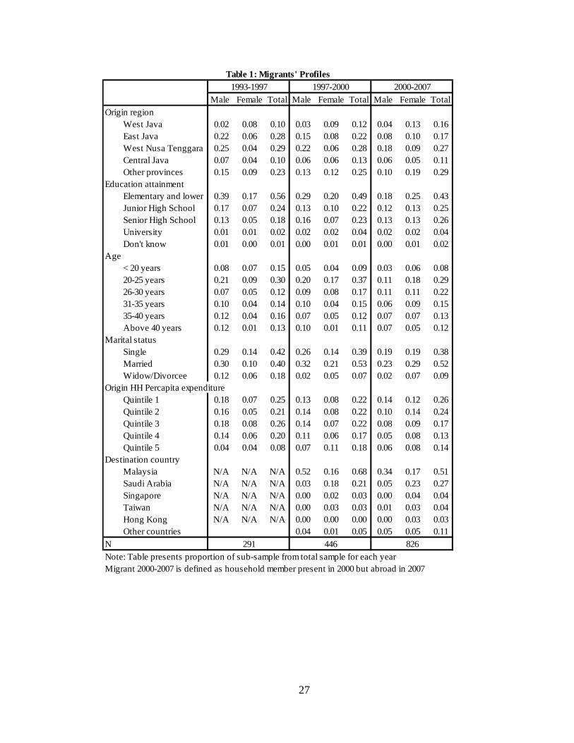
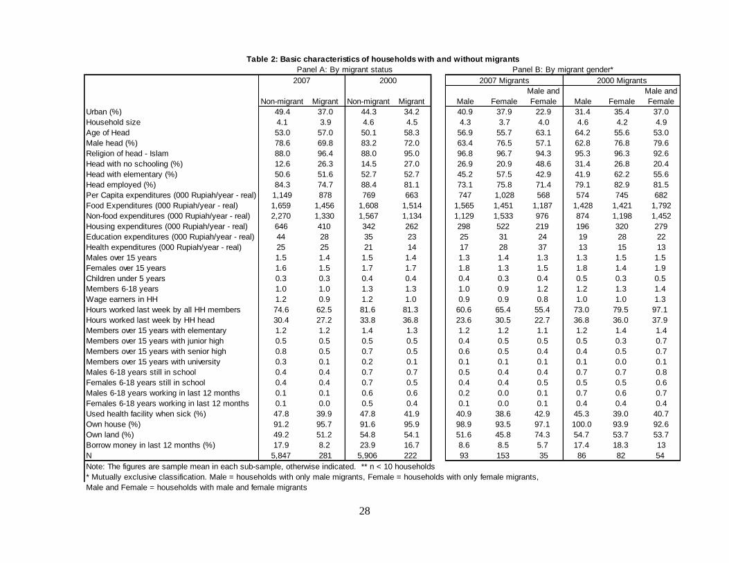
well as migrant and non-migrant households are presented in Tables 1 and 2. A simple

regression to identify correlates of migration is presented in Table 3.

The majority of Indonesian migrant workers are married and from the age group of 21

to 30 years old. On average, male migrants are older than female migrants. Interestingly,

more recent female and male migrants are both older than in previous years. The average

age of female (male) migrants in 2000-2007 was 28.7 (31.2) years old, while in 1997-

2000 was 26.8 (30.5) years old.

Migrant workers tend to be more educated than before. During the period of 1993-

2000, about half of migrant workers had primary education. However, during the

subsequent period of 2000-2007, more workers with higher levels of education found

work abroad. The proportion of migrants with junior and high school education during

2000-2007 was 9 and 6 percentage points higher than that proportion during 1993-1997

and 1997-2000, respectively. For female migrants, the proportion of senior high

education workers increased more, particularly for the last period, although the

proportion of migrants who completed senior high school was still lower than those

completed junior high school. The trend to send more educated female workers is

possibly related to demand from new destination countries for slightly more skilled work,

such as baby sitter and care taker for the elderly rather than the demand for domestic

worker. In contrast, male migrant workers experienced higher increase in the level of

junior high education over time; however, the proportion of workers having senior high

education is higher in a given year.

Indonesia migrants generally find employment in neighboring Asian countries and in

the Middle East, of which Malaysia and Saudi Arabia are the two main destinations.

While demand from these two countries continues to stay strong, the number of

destination countries in Asia is expanding. Almost 90 percent of all migrant workers

moved to Malaysia and Saudi Arabia for work during 1997-2000. This fraction

decreased to about 80 percent of all Indonesian migrant flows by 2000-2007. Female and

male migrants, however, are choosing different destinations. Although most female

migrant workers work in Saudi Arabia, they are increasingly finding employment in other

9

Asian countries, such as Malaysia, Singapore, Taiwan and Hong Kong. The trend is the

opposite for men. Although the majority of male migrants find work in Malaysia, they are

now increasingly shifting to Saudi Arabia.

About 4 to 5 percent of all sample households in the IFLS survey reported having

international migrants. The migrant sending households, however, are concentrated in

some provinces such as West Nusa Tenggara, West Java and East Java. In these

provinces, the share of sample households with migrants in 2007 was as high as 17

percent (Nusa Tenggara) and 6 percent (West and East Java). While female migrants are

predominantly from West Java, male migrants mostly come from West Nusa Tenggara.

The shares of migrants from these two main regions are increasing over time.

Although Indonesia migrant workers are increasingly coming from urban areas, the

majority of them still come from rural areas. More than 60 percent of migrant workers,

during the 2000-2007 period, still came from rural households. The new urbanizing trend

is continuing possibly as the Indonesian population is urbanizing, and increasingly more

workers from urban areas are finding work abroad. The share of households having

migrant workers from urban areas increased from 34 percent in 2000 to 37 percent in

2007. The urbanizing trend is observed stronger for households with only male migrants,

with the share from urban area rising from 31 percent in 2000 to 41 percent in 2007.

Households with migrants have, on average, significantly less per capita total

expenditure than those without migrants. From 1993 until 2000, almost equal shares of

migrant workers came from quintiles 1 to 4. Recently, the highest share of migrant

workers came from the poorest quintile of households. Migrant workers from these

households look for work outside of Indonesia in order to better financially support their

families back home. Households having only male migrants are generally worse off but,

interestingly, on average, have higher food expenditure than female migrant households.

Meanwhile, households with female migrants tend to have higher expenditure on non-

food items, particularly housing, education and health.

Interestingly, when household welfare is assessed using assets owned by the

household, the proportion of households owning house and land is higher among

households sending migrants than among non-migrant households. Similarly, the

proportion of migrant households that borrowed money in last 12 months is less than that

10

of non-migrant households. Such welfare measures, when not assessed in lags, may

indicate the use of remittances sent by household members currently overseas.

Relative to non-migrant households, households sending migrants are typically

headed by those of older age and having lower levels of education. Female migrants

come from households with younger heads, compared to male migrants. Both female and

male migrants, however, mostly come from households whose head has primary school

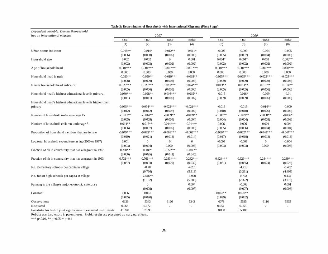
education. As can be seen in Table 3, older household heads significantly increase the

probability of the corresponding household to have an international migrant, while higher

educational attainment of the household head makes it less likely to send member to work

overseas.

Although most household heads are employed, the proportion of household heads

with employment is found less in migrant households. Among migrant households, this

proportion is always higher for female than male migrant households. Looking at the

number of wage earners in each household, non-migrant households have a higher

average number of wage earners than migrant households. As a result, the average

number of hours worked (during the last week) by the head and other members of

households with migrants is likely to be lower than that in households without migrants.

Female migrant households have higher average hours worked than those with male

migrants.

Other demographic characteristics of household members, such as household size,

number of household members above 15 years old and their education attainment, tend to

be different between households with and without migrants. On average, household

migrants tend to have fewer household members with education, particularly senior high.

Households sending migrants, both male and female migrants, also tend to have smaller

household size and a smaller number of household members above 15 years old. The

regression results in Table 3 show that an additional male household member above age

15 significantly reduces the probability of the household to have an international migrant

by about 0.9 percentage points. The higher the proportion of female household members,

the less likely that the household has an international migrant.

In general, rural areas often lack information, including that related to job

opportunities. Yet, most international migrants are from rural areas. This is because the

11

decision to take overseas jobs is partly due to networks, i.e. it is driven by success stories

of returning migrant workers who benefit from higher salaries offered in migrant

recipient countries. The regression results shown in Table 3, controlling for multivariate

correlations, show that an increase in the proportion of household with migrants in a

village from previous periods (as a proxy for network) significantly increase the

likelihood of household sending migrants in the current period.

Remittances from migrant workers are an additional source of external financing for

recipient families. The data shows that poorer households are more likely to receive

remittances. Consistent with the profiles of households sending migrants, households

receiving remittances tend to be mostly rural, having more assets, and headed by those of

older age, lower education level and less likely to have jobs.7

Over time, remittances became increasingly important, particularly in households

with female migrants. The fraction of households receiving remittances from female

migrants increased, but the fraction of households receiving remittances from male

migrants stayed roughly the same. Moreover, the average share of remittances to

household expenditure from females has also increased, while the average share from

male migrants decreased.

5. Empirical Strategy

This section discusses the methodological challenges and our approach used to

estimate the extent to which migration and remittances, differentially by gender, affect

sending households’ child outcomes and labor supply behavior.

5.1 Endogeneity

A problem commonly faced in estimating the causal impact of migration and

remittances is endogeneity. Running a simple OLS regression of household outcomes

with migration status or remittance receipts as explanatory variables could give a biased

estimate of the impact. The error term and the explanatory variable are likely correlated

due to several reasons such as reversed causality, omitted variables or selection bias.

7 The tables of descriptive statistics and determinants of households receiving remittances are not presented

as they are very similar and consistent with those households having migrants. The tables can be obtained

from the authors.

12

Unobservable characteristics that are omitted from the analysis such as ability or well-

connectedness may be correlated with both the explanatory variables—migration and

remittances—and the outcomes of interest. The direction of the bias is unclear a priori.

Ideally, an unbiased estimate of the causal impact would be the difference between

outcomes of households with migrants (and/or remittances) and their outcomes in the

counterfactual scenario when these same households do not have migrants. However,

households with migrants tend to be ―selected‖ based on unobservable characteristics.

Therefore, households without migrants will not be a good counterfactual for them.

One method to potentially account for such possible biases is the use of panel data to

perform fixed-effects or first-difference estimation. The panel data structure allows us to

control for unobserved fixed heterogeneity using household fixed effects. However, the

identification assumption would be that there are no time-varying unobservable

determinants of the outcome variables. We are concerned that there might be unobserved

shocks, such as changes in the structure of the economy or weather shocks, which

correlate with the migration decision as well as child outcomes and labor supply of the

origin household.

Another method, the instrumental variable approach, will be used to separate the

impact of migration from selection effects. Historical migration networks, defined as the

percentage of households in the village with migrants in the past, will be used as

instruments for migration and remittances in estimating their impact on the sending

households. We expect that larger initial migration networks would lower the cost of

subsequent migration, through information or through financing, and thus induce more

migration. The first-stage regression reported in Table 3 confirms this relationship. The

bottom row shows that 1993 and 1997 migration rates are very strong determinants of

whether a household has a migrant in 2007 (as well as whether a household receives

remittances). The F-statistic of joint significance of the instruments is reported at 38 or

higher. By living in a community with high levels of migration in the 1990s, a household

has a higher probability of having an international migrant than similar households in

community with lower initial migration rates. For the 2000 regressions, we use only the

1993 network as the instrument since it can be difficult to argue for using the 1997

migration rate as historical networks in the year 2000.

13

The identification assumption in this instrumental method is that past migration

networks do not influence household outcomes directly other than through their

likelihood of having a migrant member. While the validity of instruments is usually

argued and not easy to verify, we support the identification strategy in this paper in two

ways. First, tests for over-identification in the 2007 analysis fail to reject that excluded

instruments are exogenous. P-values of Sargan’s over-identification tests are reported.

Second, it is important to consider possible threats to the exclusion restriction. Past

migration with remittance inflows might have affected local levels of human and physical

capital intensity, possibly affecting labor demand or infrastructure level and local

economic development in general. These factors in turn might affect schooling and work

decisions now. To gain insights about these possible channels, we investigated the raw

and conditional correlations between various measures of local development in 2007 with

1993 and 1997 migration rates. Since correlations exist for some variables of local

development but not others, and since they do not tell a coherent story, we control for

these variables in our regressions. However, if current migration also results in greater

development, such over-controlling might not capture the full impacts of migration. In

the end, our analysis checks for robustness with and without these various controls.

5.2 Estimating Equations

The base estimating equation is, for each household i at time t = 2000 or 2007

(1) Y_it = alpha*X_it + beta*M_it + gamma*female_it*M_it + delta*

female_it + μ_it

The outcomes of interest, Y_it, include hours worked for remaining household

members, household head employment status, children’s school enrollment, and child

labor supply. X is a set of household characteristics, which can include household

composition, log of per capita expenditure (lagged), asset information (land and house

14

ownership), and community characteristics (fraction of population working in agriculture,

access to schools and roads, and so on8). μ is the unobserved component for household i.

M is an indicator for having a migrant or receiving remittances. To account for

potential endogeneity, in the two-stage least squares regressions, 1993 and 1997

migration networks, defined as the percentage of households in the village with migrants,

will be used as instruments for M in 2007. Only 1993 network will be used as instrument

for M in the 2000 equation.

As female migration may have a differential impact on the outcomes, we include

―female_it‖—a dummy variable which denotes households with only female migrants,

the omitted category being those households with at least some male migrants.

Alternatively, this variable can refer to the female share among migrants, for each

household with migrants. The coefficients of interest related to the impacts of migration

are beta and gamma. Gamma, in particular, captures the differential impact of female

migrants.

For robustness check, we will present estimations of probit model in addition to linear

probability for binary variables and also estimate a non-linear relationship in the form of

IV probit in estimating the probability of household head being employed, which is a

binary outcome. We will discuss the robustness of the results with respect to various

control variables.

6. Results

This section first presents the estimated impacts on labor supply and child outcomes,

and how the impacts vary with the gender of the migrant. The results for migration and

remittances are interpreted together throughout this section.9 This is because the results

for migration and remittances are qualitatively very similar. Also, households receiving

international remittances identified in the data are a strict subset of households with

international migrants, therefore constituting a smaller number of observations.

Subsequently, a discussion of robustness of the base results follows. The main results are

8 Other proxies for community characteristics that have been controlled for in checking for robustness in

the estimations are village home ownership rate, access to clean water, existence of a bank in the village,

existence of a slum area in the village, and electricity coverage. 9 The full set of remittance results, though not all presented, is available from the authors upon request.

15

reported for 2007, the year for which we could use two instruments, test for over-

identification, and interpret the results with more confidence. The results for 2000, the

year for which only 1993 network was used as an instrument for migration, are discussed

in the robustness sub-section. The last sub-section provides a discussion of the results.

6.1 Do Migration and Remittances Affect Labor Supply?

Migration and remittances are likely to have consequences for the welfare of sending

households through their impacts on wages and labor supply decisions. When a large

proportion of the working population migrates, this can exert an upward pressure on

wages and create work incentives for certain sectors of the labor force in sending

countries. However, impacts on the equilibrium wage are unlikely in Indonesia since the

rate of migration as a share of the large labor force is still modest, despite recent

increases in migrant outflows. Even without a change in the equilibrium wage, migration

and remittances can still affect the work decision of non-migrating family members. For

example, with the net additional income from remittances, they may opt to work less and

consume more leisure.

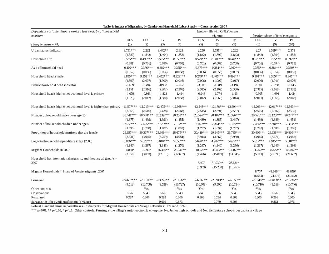
Table 4 presents the results for hours worked last week by all household members in

2007. OLS regression results, with or without controlling for various local development

variables, as shown in the first two columns, suggest that migrant-sending households

tend to work less than non-migrant households (also controlling for household size).

When we use historical migration networks as instruments for having a migrant in

2007, the above negative effect found in the OLS still hold (Columns 3 and 4), although

the size of the effect detected under the IV is larger. Migrant-sending household

members work 26 hours less per week, compared to the average 75 hours worked among

households without migrants.10

The impact of receiving remittances in 2007 is similar.

This estimate of the effect of migration and remittances on household labor supply has

both statistical and economic significance. As also shown in Table 4, the Sargan’s test

for over-identification of the instruments in the 2007 IV estimation does not reject the

10

The censored regression (tobit), under the assumption that hours worked are censored below zero, gives

similar results.

16

null hypothesis that both instruments are exogenous (p-values range from 0.619 to

0.976).

Considering the different effect by gender, we find that households with female

migrants do not reduce their work efforts while households with male migrants do.

Columns 5 to 10 of Table 4 show the differential impacts when households have more

female migrants compared to male migrants. As mentioned previously, there are two

ways we can define ―female migrant households‖: (i) dummy variable which denotes

households with only female migrants, the omitted category being those households with

at least one male migrant11

(columns 5-7); and (ii) the female share among migrants for

each household with migrants (columns 8-10).

The coefficient of interest is that of the interaction terms, interpreted as the

differential impact of migration between when the household has mostly female migrants

versus when it has mainly male migrants. This number is small and insignificant under

OLS regressions but rather large and significant under IV regressions. In column 7, for

example, the estimated coefficient is -33.402 for the Migrant Households term, and

31.939 for the interaction term ―Households has international migrants, and they are all

female.‖ Both of them are statistically significant and large. That means, while

households with predominantly male migrants work 33 hours less per week than non-

migrant households, this effect is reverted toward zero among households with female

migrants. Column 10 also tells a similar story. Households with all male migrants work

45 hours less than non-migrant households, but this effect is reverted toward zero as the

share of female migrants from the household increases. Again, the influence of receiving

remittances is very similar to the influence of having a migrant.

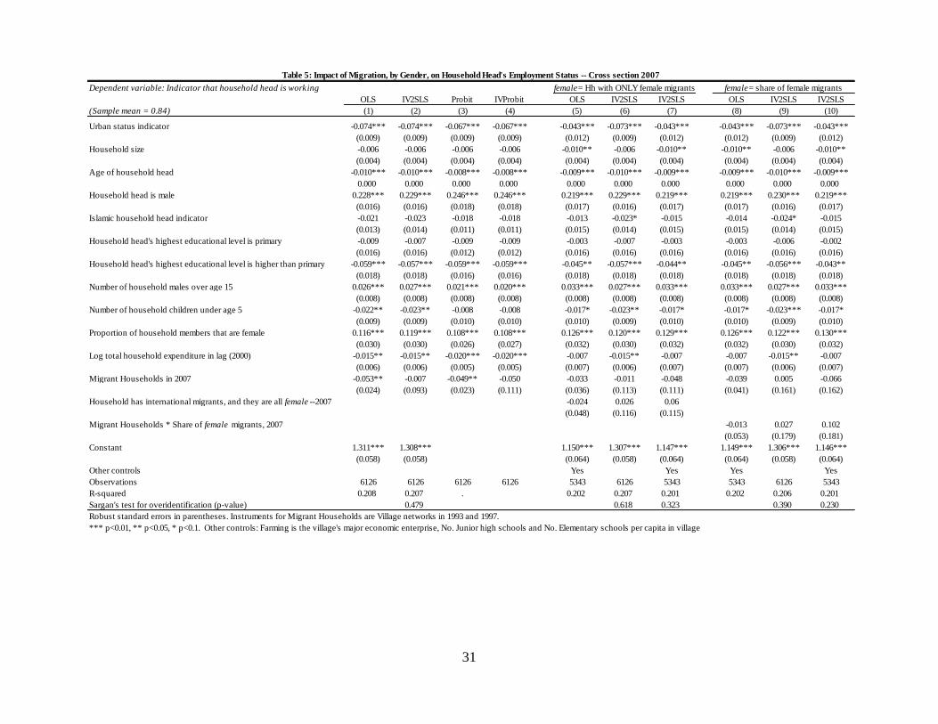
Does migration also affect the extensive margin of the decision to work, in addition to

how much to work? Table 5 analyzes factors affecting the probability that the household

head is currently working. The head is more likely to be working in rural households

(probably self-employed in agriculture), when the head is male, and when the household

is previously poor. Unconditional averages suggest that household heads with higher

11

There are very few households with migrants of both genders. We also have the results for all three

categories: female migrants only, male migrants only, and both genders. The results remain the same: any

differential impacts are between households with only female migrants and those with only male migrants.

17

education are slightly more likely to be working. However, this observation does not

hold in the regression results.

Regarding the impact of migration, while the OLS and probit regressions for this

outcome variable suggest that household heads in migrant-sending households are

significantly less likely to be employed, the instrumental variable approach shows that

this coefficient is insignificant. Column 4 reports the IV probit results since using 2SLS

for a binary outcome variable and binary endogenous variable might yield inconsistent

estimates. The zero effect on employment by the household head is observed regardless

of the migrant’s gender, as female interaction terms are small and indistinguishable from

zero. Migration does not appear to influence the household head’s likelihood of working,

even though it reduces the household head’s hours worked (not reported), similar to the

result on hours worked for all members.

6.2 Do Migration and Remittances Affect Children’s Schooling and Work Behavior?

The next set of outcome variables relates to children’s schooling and work behavior.

These regression analyses refer to children 6 to 18 years old, thus a smaller sample of

households with children.

First, as presented in Table 6, the dependent variable is the fraction of children 6-18

years old in the household that are in school in 2007. Children in urban and richer

households with a more educated household head, unsurprisingly, have higher

engagement in education.

While the OLS regression for this outcome variable (column 1) suggests that children

in migrant-sending households are more likely to be in school, the instrumental variable

approach shows that this coefficient is much smaller and insignificant. Migration has no

statistically significant effects on children’s school enrollment in Indonesia.12

The point

estimates of the ―migrant households‖ coefficient in the IV regressions (columns 3 and 4)

are closer to zero and with larger standard errors. This finding holds whether or not we

control for log of per capita expenditure or community-level development (including the

village school supply), and whether or not the household is in urban or rural areas.

Thus, only looking at OLS regressions would give a biased estimate of the effect of

12

The results do not depend on the gender of the children. They are similar for boys’ and girls’ enrollment.

18

migration. Even though the OLS regressions control for wealth and other pre-determined

characteristics, migrant-sending households might correlate with some unobservables

such as connectedness, which also affects investment in education.

Interaction terms with female migrants indicate that households with more female

migrants show almost no difference in explaining the fraction of all children enrolled in

school, as shown in columns 5-10. This finding holds for the indicator for households

with only female migrants, and the female share among migrants. Even though the sign is

oftentimes negative, the point estimates are small and insignificant.

Second, as presented in Table 7, the dependent variable is the fraction of children 6-

18 years old in the household that are working in the last 12 months of the 2007 survey.

The sample average indicates that 17% of children work, probably in family business or

informal jobs. Children in urban households with Islamic and educated head are less

likely to work in the labor market.

The OLS regression for this outcome variable suggests that children in migrant-

sending households are significantly less likely to work, whether or not controlling for

community variables. As shown in column 1, the share of children in migrant households

who work is 7 percentage points less than that in non-migrant households. This finding

becomes more nuanced when we use the instrumental variable approach. The

coefficients on the ―migrant households‖ variable, reported under columns 3 and 4, are

not distinguishable from zero.

Columns 5-10 of Table 7 show that the coefficient of the gender interaction term is

robustly negative. We find that children work less when it comes to households with

more female migrants. This finding holds for the indicator for households with only

female migrants, as well as the female share among migrants. To interpret column 6, for

example, households with only female migrants reduce the share of children working by

32 percentage points more than the impact of households with at least some male

migrants. The coefficients of ―Migrant Households‖ variable, reported in the IV

regressions (Columns 9 and 10), are positive but indistinguishable from zero. It is

inferred that migration has no statistically significant effect on child labor supply in

families with only male migrants. However, households with only female migrants

reduce the share of children working by 26.8 – 43.8 = 17 percentage points, as indicated

19

by the coefficients of the interaction terms in column 10. This effect is relatively large

and important given the sample average that 17% of children work on average in the full

sample of households.

6.3 Discussion of Robustness

Various exercises for robustness checks generally support the cross-sectional results

presented above. First, to address worries about household and community

characteristics omitted from the base regression, we checked additional specifications

controlling for these variables. The results are robust to controlling for land and house

ownership as proxies for asset holdings, indicator for having a bank in the village, village

home ownership rate (except the household in question), infrastructure such as road,

market access, access to clean water, and the presence of slums in a village. Taking into

account all fixed effects at the district level, by including district dummies, gives

qualitative similar results even though the standard errors tend to be larger due to smaller

sources of variation, unsurprisingly.13

Second, in an attempt to improve precision, additional analysis was performed in a

restricted sample of the major migrant-sending provinces. The small capture of migrant

households in the IFLS, 5% or less in the full sample, is a sample size concern and is

likely to lead to imprecise estimates. Restricting the analysis to major migration

provinces can bring the migration rate up to roughly 8% in 2007, but at the cost of a

much lower number of observations. In the end, most analysis in the restricted sample

turned out not to improve precision. The results for the restricted sample are available

upon request, but only those for the full sample are reported. In addition to robust

standard errors, bootstrapping standard errors gave similar results. Standard errors

clustered at the village level tend to be slightly larger, but also gave qualitative similar

results.

Third, the same analysis for 2000 suggests broadly similar results, except for those

about child labor supply. For 2000, only 1993 network could be used as an instrument

13

The only additional control that seems to affect some of the results is the fraction of households in the

village with electricity. This is a concern only to the extent that one argues electricity coverage affects

household labor supply and children’s school and work behavior, and is correlated with historical

migration. Even so, it is not clear if this is a good control variable since the relationship between access to

electricity and hours worked, for example, can be reversed causality.

20

for migration, and an over-identification test was not possible. Assuming the 2000 IV

specification is valid, the only difference in the 2000 results is that households with

female migrants in 2000 are not likely to lead to a reduction in child labor supply.

Finally, in addition to the cross-sectional analysis, panel analysis using household

fixed effects usually gives very high standard errors and thus imprecise, insignificant

point estimates. As one exception, assuming that there are no unobserved time-varying

determinants of the outcome variables, panel analysis does show that migration reduces

child labor supply.

6.4 Discussion of the Results

Consistent with income theory and with findings in other countries, we find that in

Indonesia, migration has a negative impact on the average labor supply of remaining

household members. This impact manifests through the intensive margin that remaining

members work fewer hours, rather than through the extensive margin that the household

head withdraws from the labor force. When disaggregated by region, Table 8 reports the

results of the IV estimations separately for urban and rural areas. In urban areas, we find

a negative effect of migration on total labor supply, regardless of the gender of the

migrant. However, the main findings about the gender influence in the whole sample

reflect closely what happens in rural areas since more migrants come from rural areas.

As indicated in column 2, male migrants tend to reduce remaining household members'

labor supply in rural areas, but female migrants do not. Moreover, the negative impact

of female migration on children’s work behavior is only observed in rural areas.

The negative impact of remittances on the labor supply of remaining household

members is not necessarily a concern unless work incentives are also distorted. The part

of the fall in labor supply due to an income effect, via increased leisure, represents a

private welfare gain. Alternatively, household members might substitute wage labor with

more time in parenting and home production, or increased capital and improved labor

productivity. On the other hand, remittances seen as conditional on low household

income can discourage work incentives of non-migrating members. It is, unfortunately,

difficult to empirically separate out the distortionary effect on labor supply. But we

know that a long-term impact on welfare may be limited if remittance recipients continue

21

to depend on external transfers and do not use remittance money for productive

investment that can bring returns in the future.

The difference in impacts on labor supply, as discussed earlier, seem to be driven by

the migrant’s gender, and his or her influence on household decisions, rather than who is

left to lead the household. Considering gender of the household head, we do not find

any evidence that the impact of migration varies significantly whether the head is male or

female. Thus, it is not the case that because women leave, the men manage the

household and use remittance money differently. One could expect that the physical

absence of and the remittances sent by migrants play a complex role in influencing their

say in household decision making. For that reason, male and female migrants may be

expected to have differential impacts on the work-leisure decision of remaining

household members.

Concerning children’s schooling, we find that migration has no statistically

significant effects on school enrollment in Indonesia. This finding is not likely explained

by supply factors. Inadequate supply of schools is not a serious concern in Indonesia at

the primary level, and to a lesser degree, at the secondary level. Our analysis shows that

even in urban areas, with better school supply, there is no evidence of impact of

migration on school enrollment. Estimated impacts on children’s school enrollment are

reported in columns 3 and 4 of Table 8. Then, is it possible that enrollment is not

responsive to migration and remittances, but school attendance may be? Column 4 of

Table 9 shows no statistically significant impact of migration on children’s hours in

school per week. In this context, the negative effect of an absent parent on childcare at

home and the ―signaling effect‖ about the returns to education may play a role in

offseting the income effects from remittances. Half of the migrants from Indonesia are

primary school graduates. And to the extent that the process and prospect of migration

leads families to revise their perceived returns to education, migration might not

necessarily increase school enrollment in the end in a country where the primary

enrollment rate is already more than 90 percent.

Does the lack of impact on education outcomes for the average household hide

differential effects among richer and poorer families? Migration and remittances can be

expected to influence poor households more due to the extent of credit constraints or

22

varying preferences for education. However, our analysis (not shown) does not find

heterogeneous effects for different levels of household expenditure.

Since the factors shaping education decisions for children in primary, secondary, and

tertiary school age can vary widely, additional analysis is conducted separately for

individuals in these age groups. The first three columns of Table 9 present these results

of impacts on enrollment. Even though the direction of the impact of migration on school

enrollment appears positive for all age groups (column 1), such a conclusion is not

evident since the empirical estimates cannot be distinguished from zero. Subject to this

caveat about imprecise estimation, the size of the impact tends to be larger among older

children aged 11 to 18 and smaller among children aged 6 to 10, whose initial enrollment

rate is already high. The positive sign of the estimated impacts reflect what happens

among households with male migrants rather than among those with female migrants, as

shown in columns 2 and 3 of Table 9. The type of families sending male migrants and

the type sending female migrants may be different for unobserved reasons, or

alternatively, male and female migrants themselves have different impacts. Since women

tend to be more involved than men in child care and monitoring children’s activities,

when a mother migrates for work overseas, this action can have worse consequences for

children’s schooling behavior than the father’s migration. In fact, columns 7-9 of Table 9

suggest that migration may increase children’s idle time among families with a migrating

female, particularly for young children aged 6-10.

These results are very similar to findings about female migration and child outcomes

in rural El Salvador. Acosta (2011) finds that male migration has null to slightly positive

effect on children’s school enrollment while female migration appears to have the

opposite effect. At the same time, female migration tends to reduce child labor, in

contrast to male migration from El Salvador. The results are also consistent with the

findings of Guzman et al. (2007) and Pfeiffer and Taylor (2007) that female migration, as

opposed to male migration, is associated with lower household expenditure on education

7. Conclusion

Using the large IFLS data, this paper is the first attempt to quantitatively assess the

impacts of migration, differentiated by gender, from Indonesia on labor supply and child

23

outcomes in sending households. We apply the instrumental variable method using

historical migration networks as instruments for migration and remittance receipts.

Overall, we find that the impacts of migration are likely to vary depending on the

gender of the migrants. Migration and remittances reduce the labor supply of remaining

members in sending households. However, this result reflects what happens in cases of

families with male migrants only. Families with female migrants may be different for

unobserved reasons, or female migrants may prefer a different use of their remittances

rather than increased leisure for adults. One possible use is to pull children out of the

labor force. Our analysis indeed shows that international migration reduces child labor

supply in households with female migrants.

Migration does not seem to significantly affect the school enrollment or attendance of

children of either gender or across age groups in Indonesia. This result is consistent with

the negative effect of an absent parent on childcare at home and the possible ―signaling

effect‖ about the returns to education that may offset the income effects from remittances.

The negative effect of an absent parent is likely to be more severe in the case of female

migrants since women tend to be more involved than men in child care and monitoring

children’s activities. Results show that migration increases children’s idle time among

families with a migrating female, particularly for young children aged 6-10, and probably

reverts any positive impact that migration may have on school enrollment.

More quality data on migration and policy evaluations would be needed to better

understand the exact mechanisms of how migration and remittances affect child

outcomes as well as other development outcomes. Given the different gender roles and

preferences in the household, further quantitative analysis is also required to obtain more

empirical evidence to understand and unpack the differential impacts by gender.

Assessing the net impact on welfare and the long-term consequences of migration and

remittances would require looking more comprehensively at other economic and social

outcomes likely affected by this process.

24

REFERENCES

Acosta, P. (2011). ―Female Migration and Child Occupation in Rural El Salvador.‖

Forthcoming in Population Research and Policy Review.

Acosta, P. (2006). ―Labor Supply, School Attendance, and Remittances from

International Migration: The Case of El Salvador.‖ World Bank Policy Research

Working Paper 3903.

Acosta, P., P. Fajnzylber and J. Humberto Lopez (2008). ―Remittances and Household

Behavior: Evidence for Latin America,‖ in P. Fajnzylber and J. Humberto Lopez

(eds) Remittances and Development: Lessons from Latin America. Washington, DC:

World Bank.

Adams, R. (2010) ―Evaluating the Economic Impact of International Remittances on

Developing Countries Using Household Surveys: A Literature Review.‖

Forthcoming in Journal of Development Studies.

Adams, Jr., R. (1998). ―Remittances, Investment and Rural Asset Accumulation in

Pakistan,‖ Economic Development and Cultural Change 47:1 (October): 155-173.

Adams, R. and A. Cuecuecha (2010). ―The Economic Impact of International Migration

and Remittances on Poverty and Household Consumption and Investment in

Indonesia.‖ World Bank, Washington DC.

Beaudouin, P. (2005). ―Economic Impact of Migration on a Rural Area in Bangladesh.‖

Mimeo, Centre d’Economie de la Sorbonne, Universite Paris 1.

Buchori, C. and M. Amalia (2006). ―Fact Sheet: Migration, Remittance and Female

Migrant Workers.‖ World Bank, Washington DC.

Cabegin, E. (2006). ―The Effect of Filipino Overseas Migration on the Non-Migrant

Spouse’s Market Participation and Labor Supply Behavior.‖ Institute for Study of

Labor (IZA) Discussion Paper 2240. Bonn, Germany.

Guzman, J., A. Morrison and M. Sjoblom (2008). ―The Impact of Remittances and

Gender on Household Expenditure Patterns: Evidence from Ghana‖ in A. Morrison,

M. Schiff, and M. Sjoblom (eds) The International Migration of Women. The World

Bank, Washington, DC.

Halliday, T. (2008). ―Migration, Risk and the Intra-Household Allocation of Labor in El

Salvador.‖ The University of Hawaii.

Hanson, G. (2008). ―International Migration and Development.‖ Working Paper #42,

Commission on Growth and Development, World Bank, Washington DC.

25

Mansuri, G. (2006a). ―Migration, School Attainment and Child Labor: Evidence from

Rural Pakistan.‖ World Bank Policy Research Working Paper 3945.

Mansuri, G. (2006b). ―Migration, Sex Bias, and Child Growth in Rural Pakistan.‖ World

Bank Policy Research Working Paper 3946.

Mansuri, G. (2007). ―Temporary Migration and Rural Development,‖ in C. Ozden and

M. Schiff (eds) International Migration Policy and Economic Development: Studies

Across the Globe. Washington, DC: World Bank.

McKenzie, D. and M. Sasin (2007). ―Migration, Remittances, Poverty, and Human

Capital: Conceptual and Empirical Challenges.‖ World Bank Policy Research

Working Paper 4272.

McKenzie, D. and H. Rapoport (2006). ―Can Migration Reduce Educational Attainment?

Evidence from Mexico.‖ World Bank Policy Research Working Paper 3952,

Washington DC.

National Commission for the Placement and Protection of Indonesian Migration Workers

(BNP2TKI), 2009.

Pfeiffer, L. and J.E. Taylor (2008). ―Gender and the Impacts of International Migration:

Evidence from Rural Mexico‖ in A. Morrison, M. Schiff, and M. Sjoblom (eds) The

International Migration of Women. The World Bank, Washington, DC.

World Bank (2008a). The International Migration of Women, edited by A. Morrison, M.

Schiff, and M. Sjoblom. Washington, DC.

World Bank (2008b). ―The Malaysia-Indonesia Remittance Corridor.‖ World Bank

Working Paper No. 149. Washington, DC.

Yang, D. (2008). "International Migration, Remittances and Household Investment:

Evidence from Philippine Migrants' Exchange Rate Shocks." Economic Journal,

Royal Economic Society, vol. 118(528), pages 591-630, 04.

Yang, D. and H. Choi (2007). ―Are Remittances Insurance? Evidence from Rainfall

Shocks in the Philippines.‖ The World Bank Economic Review (May).

26

Figure 1

Flow of number of migrant workers by sex

0

100000

200000

300000

400000

500000

600000

1994

1996

1998

2000

2002

2004

2006

Male

Female

Source: BNP2TKI

27

Male Female Total Male Female Total Male Female Total

Origin region

West Java 0.02 0.08 0.10 0.03 0.09 0.12 0.04 0.13 0.16

East Java 0.22 0.06 0.28 0.15 0.08 0.22 0.08 0.10 0.17

West Nusa Tenggara 0.25 0.04 0.29 0.22 0.06 0.28 0.18 0.09 0.27

Central Java 0.07 0.04 0.10 0.06 0.06 0.13 0.06 0.05 0.11

Other provinces 0.15 0.09 0.23 0.13 0.12 0.25 0.10 0.19 0.29

Education attainment

Elementary and lower 0.39 0.17 0.56 0.29 0.20 0.49 0.18 0.25 0.43

Junior High School 0.17 0.07 0.24 0.13 0.10 0.22 0.12 0.13 0.25

Senior High School 0.13 0.05 0.18 0.16 0.07 0.23 0.13 0.13 0.26

University 0.01 0.01 0.02 0.02 0.02 0.04 0.02 0.02 0.04

Don't know 0.01 0.00 0.01 0.00 0.01 0.01 0.00 0.01 0.02

Age

< 20 years 0.08 0.07 0.15 0.05 0.04 0.09 0.03 0.06 0.08

20-25 years 0.21 0.09 0.30 0.20 0.17 0.37 0.11 0.18 0.29

26-30 years 0.07 0.05 0.12 0.09 0.08 0.17 0.11 0.11 0.22

31-35 years 0.10 0.04 0.14 0.10 0.04 0.15 0.06 0.09 0.15

35-40 years 0.12 0.04 0.16 0.07 0.05 0.12 0.07 0.07 0.13

Above 40 years 0.12 0.01 0.13 0.10 0.01 0.11 0.07 0.05 0.12

Marital status

Single 0.29 0.14 0.42 0.26 0.14 0.39 0.19 0.19 0.38

Married 0.30 0.10 0.40 0.32 0.21 0.53 0.23 0.29 0.52

Widow/Divorcee 0.12 0.06 0.18 0.02 0.05 0.07 0.02 0.07 0.09

Origin HH Percapita expenditure

Quintile 1 0.18 0.07 0.25 0.13 0.08 0.22 0.14 0.12 0.26

Quintile 2 0.16 0.05 0.21 0.14 0.08 0.22 0.10 0.14 0.24

Quintile 3 0.18 0.08 0.26 0.14 0.07 0.22 0.08 0.09 0.17

Quintile 4 0.14 0.06 0.20 0.11 0.06 0.17 0.05 0.08 0.13

Quintile 5 0.04 0.04 0.08 0.07 0.11 0.18 0.06 0.08 0.14

Destination country

Malaysia N/A N/A N/A 0.52 0.16 0.68 0.34 0.17 0.51

Saudi Arabia N/A N/A N/A 0.03 0.18 0.21 0.05 0.23 0.27

Singapore N/A N/A N/A 0.00 0.02 0.03 0.00 0.04 0.04

Taiwan N/A N/A N/A 0.00 0.03 0.03 0.01 0.03 0.04

Hong Kong N/A N/A N/A 0.00 0.00 0.00 0.00 0.03 0.03

Other countries 0.04 0.01 0.05 0.05 0.05 0.11

N

Note: Table presents proportion of sub-sample from total sample for each year

Migrant 2000-2007 is defined as household member present in 2000 but abroad in 2007

1993-1997 1997-2000 2000-2007

291 446 826

Table 1: Migrants' Profiles

28

Non-migrant Migrant Non-migrant Migrant Male Female

Male and

Female Male Female

Male and

Female

Urban (%) 49.4 37.0 44.3 34.2 40.9 37.9 22.9 31.4 35.4 37.0

Household size 4.1 3.9 4.6 4.5 4.3 3.7 4.0 4.6 4.2 4.9

Age of Head 53.0 57.0 50.1 58.3 56.9 55.7 63.1 64.2 55.6 53.0

Male head (%) 78.6 69.8 83.2 72.0 63.4 76.5 57.1 62.8 76.8 79.6

Religion of head - Islam 88.0 96.4 88.0 95.0 96.8 96.7 94.3 95.3 96.3 92.6

Head with no schooling (%) 12.6 26.3 14.5 27.0 26.9 20.9 48.6 31.4 26.8 20.4

Head with elementary (%) 50.6 51.6 52.7 52.7 45.2 57.5 42.9 41.9 62.2 55.6

Head employed (%) 84.3 74.7 88.4 81.1 73.1 75.8 71.4 79.1 82.9 81.5

Per Capita expenditures (000 Rupiah/year - real) 1,149 878 769 663 747 1,028 568 574 745 682

Food Expenditures (000 Rupiah/year - real) 1,659 1,456 1,608 1,514 1,565 1,451 1,187 1,428 1,421 1,792

Non-food expenditures (000 Rupiah/year - real) 2,270 1,330 1,567 1,134 1,129 1,533 976 874 1,198 1,452

Housing expenditures (000 Rupiah/year - real) 646 410 342 262 298 522 219 196 320 279

Education expenditures (000 Rupiah/year - real) 44 28 35 23 25 31 24 19 28 22

Health expenditures (000 Rupiah/year - real) 25 25 21 14 17 28 37 13 15 13

Males over 15 years 1.5 1.4 1.5 1.4 1.3 1.4 1.3 1.3 1.5 1.5

Females over 15 years 1.6 1.5 1.7 1.7 1.8 1.3 1.5 1.8 1.4 1.9

Children under 5 years 0.3 0.3 0.4 0.4 0.4 0.3 0.4 0.5 0.3 0.5

Members 6-18 years 1.0 1.0 1.3 1.3 1.0 0.9 1.2 1.2 1.3 1.4

Wage earners in HH 1.2 0.9 1.2 1.0 0.9 0.9 0.8 1.0 1.0 1.3

Hours worked last week by all HH members 74.6 62.5 81.6 81.3 60.6 65.4 55.4 73.0 79.5 97.1

Hours worked last week by HH head 30.4 27.2 33.8 36.8 23.6 30.5 22.7 36.8 36.0 37.9

Members over 15 years with elementary 1.2 1.2 1.4 1.3 1.2 1.2 1.1 1.2 1.4 1.4

Members over 15 years with junior high 0.5 0.5 0.5 0.5 0.4 0.5 0.5 0.5 0.3 0.7

Members over 15 years with senior high 0.8 0.5 0.7 0.5 0.6 0.5 0.4 0.4 0.5 0.7

Members over 15 years with university 0.3 0.1 0.2 0.1 0.1 0.1 0.1 0.1 0.0 0.1

Males 6-18 years still in school 0.4 0.4 0.7 0.7 0.5 0.4 0.4 0.7 0.7 0.8

Females 6-18 years still in school 0.4 0.4 0.7 0.5 0.4 0.4 0.5 0.5 0.5 0.6

Males 6-18 years working in last 12 months 0.1 0.1 0.6 0.6 0.2 0.0 0.1 0.7 0.6 0.7

Females 6-18 years working in last 12 months 0.1 0.0 0.5 0.4 0.1 0.0 0.1 0.4 0.4 0.4

Used health facility when sick (%) 47.8 39.9 47.8 41.9 40.9 38.6 42.9 45.3 39.0 40.7

Own house (%) 91.2 95.7 91.6 95.9 98.9 93.5 97.1 100.0 93.9 92.6

Own land (%) 49.2 51.2 54.8 54.1 51.6 45.8 74.3 54.7 53.7 53.7

Borrow money in last 12 months (%) 17.9 8.2 23.9 16.7 8.6 8.5 5.7 17.4 18.3 13

N 5,847 281 5,906 222 93 153 35 86 82 54

Note: The figures are sample mean in each sub-sample, otherwise indicated. ** n < 10 households

* Mutually exclusive classification. Male = households with only male migrants, Female = households with only female migrants,

Male and Female = households with male and female migrants

Table 2: Basic characteristics of households with and without migrants

Panel A: By migrant status Panel B: By migrant gender*

2007 2000 2007 Migrants 2000 Migrants

29

Dependent variable: Dummy if household

has an international migrant

OLS OLS Probit Probit OLS OLS Probit Probit

(1) (2) (3) (4) (5) (6) (7) (8)

Urban status indicator -0.015** -0.014* -0.012** -0.011* -0.005 -0.009 -0.004 -0.005

(0.006) (0.008) (0.005) (0.006) (0.005) (0.007) (0.004) (0.006)

Household size 0.002 0.002 0 0.001 0.004* 0.004* 0.003 0.003**

(0.002) (0.003) (0.002) (0.002) (0.002) (0.002) (0.002) (0.002)

Age of household head 0.001*** 0.001*** 0.001*** 0.001*** 0.001*** 0.001*** 0.001*** 0.000***

0.000 0.000 0.000 0.000 0.000 0.000 0.000 0.000

Household head is male -0.020** -0.020** -0.019** -0.018** -0.025*** -0.025*** -0.022*** -0.023***

(0.008) (0.009) (0.008) (0.008) (0.009) (0.009) (0.008) (0.008)

Islamic household head indicator 0.020*** 0.020*** 0.023*** 0.024*** 0.013** 0.011** 0.013** 0.014**

(0.005) (0.006) (0.005) (0.006) (0.005) (0.005) (0.006) (0.006)

Household head's highest educational level is primary -0.030*** -0.028** -0.016*** -0.015** -0.015 -0.016* -0.009 -0.01

(0.011) (0.011) (0.006) (0.007) (0.009) (0.009) (0.006) (0.006)

Household head's highest educational level is higher than

primary -0.035*** -0.034*** -0.022*** -0.021*** -0.016 -0.015 -0.014** -0.009

(0.012) (0.012) (0.007) (0.007) (0.010) (0.010) (0.006) (0.007)

Number of household males over age 15 -0.013** -0.014** -0.009** -0.009** -0.009** -0.009** -0.008** -0.006*

(0.005) (0.005) (0.004) (0.004) (0.004) (0.004) (0.003) (0.003)

Number of household children under age 5 0.014** 0.015** 0.014*** 0.014** 0.006 0.006 0.004 0.004

(0.006) (0.007) (0.005) (0.005) (0.005) (0.006) (0.004) (0.004)

Proportion of household members that are female -0.079*** -0.085*** -0.061*** -0.063*** -0.060*** -0.062*** -0.048*** -0.047***

(0.019) (0.021) (0.013) (0.014) (0.017) (0.018) (0.013) (0.013)

Log total household expenditure in lag (2000 or 1997) 0.001 0 0 0 -0.003 -0.003 0 -0.004

(0.003) (0.004) 0.000 (0.003) (0.003) (0.003) 0.000 (0.003)

Fraction of hh in community that has a migrant in 1997 0.200** 0.183* 0.122*** 0.101**

(0.086) (0.095) (0.041) (0.045)

Fraction of hh in community that has a migrant in 1993 0.731*** 0.761*** 0.283*** 0.282*** 0.624*** 0.629*** 0.244*** 0.239***

(0.087) (0.093) (0.029) (0.032) (0.081) (0.085) (0.024) (0.025)

No. Elementary schools per capita in village -0.78 -4.201 -4.713 -5.452

(0.736) (5.813) (3.231) (4.403)

No. Junior high schools per capita in village -2.446** -5.998 0.792 0.134

(1.132) (5.385) (2.372) (3.273)

Farming is the village's major economic enterprise 0 0.004 -0.003 0.001

(0.008) (0.007) (0.007) (0.006)

Constant 0.056 0.061 0.061** 0.070**

(0.035) (0.040) (0.029) (0.032)

Observations 6126 5343 6126 5343 6078 5535 6116 5535

R-squared 0.068 0.072 . . 0.054 0.055 . .

F-statistic for test of joint significance of excluded instruments 41.240 37.990 58.830 55.180

Robust standard errors in parentheses. Probit results are presented as marginal effects.

*** p<0.01, ** p<0.05, * p<0.1

Table 3: Determinants of Households with International Migrants (First Stage)

2007 2000

30

Dependent variable: #hours worked last week by all household

members

OLS OLS IV IV OLS IV IV OLS IV IV

(Sample mean = 74) (1) (2) (3) (4) (5) (6) (7) (8) (9) (10)

Urban status indicator 3.791*** 2.232 3.442** 2.128 2.256 3.551** 2.262 2.27 3.599*** 2.378

(1.380) (1.842) (1.404) (1.852) (1.842) (1.392) (1.843) (1.842) (1.394) (1.852)

Household size 8.535*** 8.495*** 8.595*** 8.556*** 8.529*** 8.681*** 8.640*** 8.526*** 8.725*** 8.692***

(0.681) (0.701) (0.686) (0.705) (0.701) (0.689) (0.708) (0.701) (0.694) (0.713)

Age of household head -0.402*** -0.376*** -0.382*** -0.355*** -0.375*** -0.384*** -0.360*** -0.375*** -0.384*** -0.360***

(0.052) (0.056) (0.054) (0.058) (0.056) (0.053) (0.057) (0.056) (0.054) (0.057)

Household head is male 8.895*** 9.353*** 8.452*** 8.923*** 9.279*** 8.405*** 8.896*** 9.301*** 8.365*** 8.845***

(1.890) (2.007) (1.900) (2.016) (2.006) (1.902) (2.017) (2.006) (1.911) (2.026)

Islamic household head indicator -1.699 -3.494 -0.932 -2.762 -3.508 -1.319 -3.194 -3.501 -1.298 -3.145

(2.151) (2.316) (2.202) (2.365) (2.315) (2.169) (2.330) (2.315) (2.168) (2.328)

Household head's highest educational level is primary -1.079 -0.863 -1.823 -1.494 -0.948 -1.774 -1.454 -0.905 -1.696 -1.424

(1.923) (2.012) (1.980) (2.058) (2.012) (1.965) (2.044) (2.011) (1.965) (2.048)

Household head's highest educational level is higher than primary -11.577*** -12.213*** -12.475*** -12.968*** -12.248*** -12.178*** -12.694*** -12.203*** -12.017*** -12.563***

(2.365) (2.516) (2.428) (2.568) (2.515) (2.394) (2.537) (2.515) (2.392) (2.535)

Number of household males over age 15 20.441*** 20.548*** 20.139*** 20.253*** 20.524*** 20.189*** 20.326*** 20.521*** 20.125*** 20.247***

(1.375) (1.439) (1.391) (1.455) (1.439) (1.385) (1.447) (1.439) (1.389) (1.451)

Number of household children under age 5 -7.552*** -7.455*** -7.220*** -7.132*** -7.460*** -7.364*** -7.318*** -7.464*** -7.384*** -7.333***

(1.695) (1.798) (1.707) (1.810) (1.797) (1.697) (1.797) (1.797) (1.699) (1.796)

Proportion of household members that are female 29.957*** 30.367*** 28.309*** 28.675*** 30.419*** 29.245*** 29.735*** 30.430*** 29.338*** 29.810***

(3.631) (3.945) (3.759) (4.084) (3.944) (3.667) (3.980) (3.945) (3.671) (3.982)

Log total household expenditure in lag (2000) 5.036*** 5.623*** 5.040*** 5.650*** 5.620*** 4.987*** 5.625*** 5.617*** 4.945*** 5.604***

(1.140) (1.267) (1.143) (1.270) (1.267) (1.140) (1.266) (1.267) (1.140) (1.266)

Migrant Households in 2007 -4.858* -5.993* -26.450** -26.341** -10.527** -33.402** -31.166** -11.250** -45.582** -45.102**

(2.950) (3.093) (12.310) (12.607) (4.476) (15.019) (14.945) (5.113) (21.099) (21.692)

Household has international migrants, and they are all female --

2007 8.407 31.939** 28.631*

(5.939) (15.253) (15.263)

Migrant Households * Share of female migrants, 2007 8.707 48.366** 46.859*

(6.584) (24.376) (25.432)

Constant -24.682*** -25.911** -23.276** -25.156** -26.060** -23.913** -26.056** -26.046** -23.839** -26.236**

(9.513) (10.708) (9.538) (10.727) (10.708) (9.506) (10.714) (10.710) (9.518) (10.746)

Other controls Yes Yes Yes Yes Yes Yes

Observations 6126 5343 6126 5343 5343 6126 5343 5343 6126 5343

R-squared 0.297 0.306 0.292 0.300 0.306 0.294 0.303 0.306 0.291 0.300

Sargan's test for overidentification (p-value) 0.619 0.873 0.779 0.908 0.862 0.976

Robust standard errors in parentheses. Instruments for Migrant Households are Village networks in 1993 and 1997.

*** p<0.01, ** p<0.05, * p<0.1. Other controls: Farming is the village's major economic enterprise, No. Junior high schools and No. Elementary schools per capita in village

Table 4: Impact of Migration, by Gender, on Household Labor Supply -- Cross section 2007

female= Hh with ONLY female

migrants female= share of female migrants

31

Dependent variable: Indicator that household head is working

OLS IV2SLS Probit IVProbit OLS IV2SLS IV2SLS OLS IV2SLS IV2SLS

(Sample mean = 0.84) (1) (2) (3) (4) (5) (6) (7) (8) (9) (10)

Urban status indicator -0.074*** -0.074*** -0.067*** -0.067*** -0.043*** -0.073*** -0.043*** -0.043*** -0.073*** -0.043***

(0.009) (0.009) (0.009) (0.009) (0.012) (0.009) (0.012) (0.012) (0.009) (0.012)

Household size -0.006 -0.006 -0.006 -0.006 -0.010** -0.006 -0.010** -0.010** -0.006 -0.010**

(0.004) (0.004) (0.004) (0.004) (0.004) (0.004) (0.004) (0.004) (0.004) (0.004)

Age of household head -0.010*** -0.010*** -0.008*** -0.008*** -0.009*** -0.010*** -0.009*** -0.009*** -0.010*** -0.009***

0.000 0.000 0.000 0.000 0.000 0.000 0.000 0.000 0.000 0.000

Household head is male 0.228*** 0.229*** 0.246*** 0.246*** 0.219*** 0.229*** 0.219*** 0.219*** 0.230*** 0.219***

(0.016) (0.016) (0.018) (0.018) (0.017) (0.016) (0.017) (0.017) (0.016) (0.017)

Islamic household head indicator -0.021 -0.023 -0.018 -0.018 -0.013 -0.023* -0.015 -0.014 -0.024* -0.015

(0.013) (0.014) (0.011) (0.011) (0.015) (0.014) (0.015) (0.015) (0.014) (0.015)

Household head's highest educational level is primary -0.009 -0.007 -0.009 -0.009 -0.003 -0.007 -0.003 -0.003 -0.006 -0.002

(0.016) (0.016) (0.012) (0.012) (0.016) (0.016) (0.016) (0.016) (0.016) (0.016)

Household head's highest educational level is higher than primary -0.059*** -0.057*** -0.059*** -0.059*** -0.045** -0.057*** -0.044** -0.045** -0.056*** -0.043**

(0.018) (0.018) (0.016) (0.016) (0.018) (0.018) (0.018) (0.018) (0.018) (0.018)

Number of household males over age 15 0.026*** 0.027*** 0.021*** 0.020*** 0.033*** 0.027*** 0.033*** 0.033*** 0.027*** 0.033***

(0.008) (0.008) (0.008) (0.008) (0.008) (0.008) (0.008) (0.008) (0.008) (0.008)

Number of household children under age 5 -0.022** -0.023** -0.008 -0.008 -0.017* -0.023** -0.017* -0.017* -0.023*** -0.017*

(0.009) (0.009) (0.010) (0.010) (0.010) (0.009) (0.010) (0.010) (0.009) (0.010)

Proportion of household members that are female 0.116*** 0.119*** 0.108*** 0.108*** 0.126*** 0.120*** 0.129*** 0.126*** 0.122*** 0.130***

(0.030) (0.030) (0.026) (0.027) (0.032) (0.030) (0.032) (0.032) (0.030) (0.032)

Log total household expenditure in lag (2000) -0.015** -0.015** -0.020*** -0.020*** -0.007 -0.015** -0.007 -0.007 -0.015** -0.007

(0.006) (0.006) (0.005) (0.005) (0.007) (0.006) (0.007) (0.007) (0.006) (0.007)

Migrant Households in 2007 -0.053** -0.007 -0.049** -0.050 -0.033 -0.011 -0.048 -0.039 0.005 -0.066

(0.024) (0.093) (0.023) (0.111) (0.036) (0.113) (0.111) (0.041) (0.161) (0.162)

Household has international migrants, and they are all female --2007 -0.024 0.026 0.06

(0.048) (0.116) (0.115)

Migrant Households * Share of female migrants, 2007 -0.013 0.027 0.102

(0.053) (0.179) (0.181)

Constant 1.311*** 1.308*** 1.150*** 1.307*** 1.147*** 1.149*** 1.306*** 1.146***

(0.058) (0.058) (0.064) (0.058) (0.064) (0.064) (0.058) (0.064)

Other controls Yes Yes Yes Yes

Observations 6126 6126 6126 6126 5343 6126 5343 5343 6126 5343

R-squared 0.208 0.207 . 0.202 0.207 0.201 0.202 0.206 0.201

Sargan's test for overidentification (p-value) 0.479 0.618 0.323 0.390 0.230

Robust standard errors in parentheses. Instruments for Migrant Households are Village networks in 1993 and 1997.

*** p<0.01, ** p<0.05, * p<0.1. Other controls: Farming is the village's major economic enterprise, No. Junior high schools and No. Elementary schools per capita in village

Table 5: Impact of Migration, by Gender, on Household Head's Employment Status -- Cross section 2007

female= Hh with ONLY female migrants female= share of female migrants

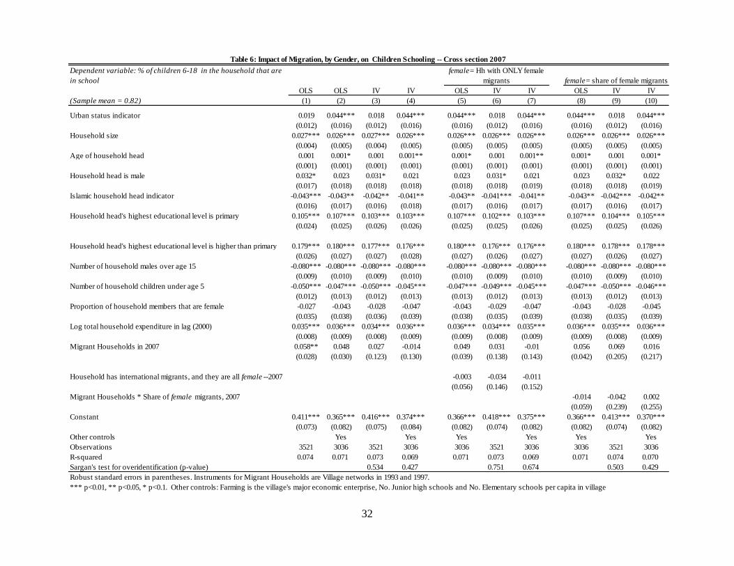
32

Dependent variable: % of children 6-18 in the household that are

in school

OLS OLS IV IV OLS IV IV OLS IV IV

(Sample mean = 0.82) (1) (2) (3) (4) (5) (6) (7) (8) (9) (10)

Urban status indicator 0.019 0.044*** 0.018 0.044*** 0.044*** 0.018 0.044*** 0.044*** 0.018 0.044***

(0.012) (0.016) (0.012) (0.016) (0.016) (0.012) (0.016) (0.016) (0.012) (0.016)

Household size 0.027*** 0.026*** 0.027*** 0.026*** 0.026*** 0.026*** 0.026*** 0.026*** 0.026*** 0.026***

(0.004) (0.005) (0.004) (0.005) (0.005) (0.005) (0.005) (0.005) (0.005) (0.005)

Age of household head 0.001 0.001* 0.001 0.001** 0.001* 0.001 0.001** 0.001* 0.001 0.001*

(0.001) (0.001) (0.001) (0.001) (0.001) (0.001) (0.001) (0.001) (0.001) (0.001)

Household head is male 0.032* 0.023 0.031* 0.021 0.023 0.031* 0.021 0.023 0.032* 0.022

(0.017) (0.018) (0.018) (0.018) (0.018) (0.018) (0.019) (0.018) (0.018) (0.019)

Islamic household head indicator -0.043*** -0.043** -0.042** -0.041** -0.043** -0.041*** -0.041** -0.043** -0.042*** -0.042**

(0.016) (0.017) (0.016) (0.018) (0.017) (0.016) (0.017) (0.017) (0.016) (0.017)

Household head's highest educational level is primary 0.105*** 0.107*** 0.103*** 0.103*** 0.107*** 0.102*** 0.103*** 0.107*** 0.104*** 0.105***

(0.024) (0.025) (0.026) (0.026) (0.025) (0.025) (0.026) (0.025) (0.025) (0.026)

Household head's highest educational level is higher than primary 0.179*** 0.180*** 0.177*** 0.176*** 0.180*** 0.176*** 0.176*** 0.180*** 0.178*** 0.178***

(0.026) (0.027) (0.027) (0.028) (0.027) (0.026) (0.027) (0.027) (0.026) (0.027)

Number of household males over age 15 -0.080*** -0.080*** -0.080*** -0.080*** -0.080*** -0.080*** -0.080*** -0.080*** -0.080*** -0.080***

(0.009) (0.010) (0.009) (0.010) (0.010) (0.009) (0.010) (0.010) (0.009) (0.010)

Number of household children under age 5 -0.050*** -0.047*** -0.050*** -0.045*** -0.047*** -0.049*** -0.045*** -0.047*** -0.050*** -0.046***

(0.012) (0.013) (0.012) (0.013) (0.013) (0.012) (0.013) (0.013) (0.012) (0.013)

Proportion of household members that are female -0.027 -0.043 -0.028 -0.047 -0.043 -0.029 -0.047 -0.043 -0.028 -0.045

(0.035) (0.038) (0.036) (0.039) (0.038) (0.035) (0.039) (0.038) (0.035) (0.039)

Log total household expenditure in lag (2000) 0.035*** 0.036*** 0.034*** 0.036*** 0.036*** 0.034*** 0.035*** 0.036*** 0.035*** 0.036***

(0.008) (0.009) (0.008) (0.009) (0.009) (0.008) (0.009) (0.009) (0.008) (0.009)

Migrant Households in 2007 0.058** 0.048 0.027 -0.014 0.049 0.031 -0.01 0.056 0.069 0.016

(0.028) (0.030) (0.123) (0.130) (0.039) (0.138) (0.143) (0.042) (0.205) (0.217)

Household has international migrants, and they are all female --2007 -0.003 -0.034 -0.011

(0.056) (0.146) (0.152)

Migrant Households * Share of female migrants, 2007 -0.014 -0.042 0.002

(0.059) (0.239) (0.255)

Constant 0.411*** 0.365*** 0.416*** 0.374*** 0.366*** 0.418*** 0.375*** 0.366*** 0.413*** 0.370***

(0.073) (0.082) (0.075) (0.084) (0.082) (0.074) (0.082) (0.082) (0.074) (0.082)

Other controls Yes Yes Yes Yes Yes Yes

Observations 3521 3036 3521 3036 3036 3521 3036 3036 3521 3036

R-squared 0.074 0.071 0.073 0.069 0.071 0.073 0.069 0.071 0.074 0.070

Sargan's test for overidentification (p-value) 0.534 0.427 0.751 0.674 0.503 0.429

Robust standard errors in parentheses. Instruments for Migrant Households are Village networks in 1993 and 1997.

*** p<0.01, ** p<0.05, * p<0.1. Other controls: Farming is the village's major economic enterprise, No. Junior high schools and No. Elementary schools per capita in village

Table 6: Impact of Migration, by Gender, on Children Schooling -- Cross section 2007

female= Hh with ONLY female

migrants female= share of female migrants

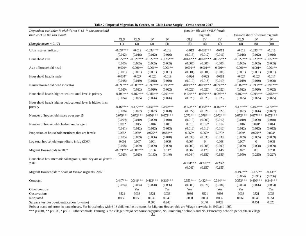
33

Dependent variable: % of children 6-18 in the household

that work in the last month

OLS OLS IV IV OLS IV IV OLS IV IV

(Sample mean = 0.17) (1) (2) (3) (4) (5) (6) (7) (8) (9) (10)

Urban status indicator -0.037*** -0.012 -0.033*** -0.012 -0.013 -0.035*** -0.013 -0.013 -0.035*** -0.015

(0.012) (0.016) (0.012) (0.016) (0.016) (0.012) (0.016) (0.016) (0.012) (0.016)

Household size -0.027*** -0.026*** -0.027*** -0.025*** -0.026*** -0.028*** -0.027*** -0.027*** -0.029*** -0.027***

(0.005) (0.005) (0.005) (0.005) (0.005) (0.005) (0.005) (0.005) (0.005) (0.005)

Age of household head -0.001* -0.001** -0.001** -0.001** -0.001** -0.001** -0.001** -0.001** -0.001* -0.001**

(0.001) (0.001) (0.001) (0.001) (0.001) (0.001) (0.001) (0.001) (0.001) (0.001)

Household head is male -0.034* -0.027 -0.026 -0.019 -0.024 -0.025 -0.018 -0.024 -0.024 -0.017

(0.018) (0.019) (0.018) (0.019) (0.019) (0.018) (0.019) (0.019) (0.019) (0.020)

Islamic household head indicator -0.090*** -0.088*** -0.097*** -0.095*** -0.087*** -0.092*** -0.090*** -0.087*** -0.093*** -0.091***

(0.020) (0.022) (0.020) (0.022) (0.022) (0.020) (0.022) (0.022) (0.020) (0.022)

Household head's highest educational level is primary -0.100*** -0.102*** -0.086*** -0.091*** -0.101*** -0.091*** -0.095*** -0.102*** -0.093*** -0.096***

(0.024) (0.025) (0.026) (0.026) (0.025) (0.025) (0.025) (0.025) (0.025) (0.025)

Household head's highest educational level is higher than

primary -0.163*** -0.172*** -0.151*** -0.160*** -0.172*** -0.158*** -0.167*** -0.173*** -0.160*** -0.170***

(0.026) (0.027) (0.027) (0.028) (0.027) (0.026) (0.027) (0.027) (0.026) (0.027)

Number of household males over age 15 0.075*** 0.072*** 0.076*** 0.073*** 0.072*** 0.076*** 0.072*** 0.072*** 0.077*** 0.073***

(0.009) (0.010) (0.009) (0.010) (0.010) (0.009) (0.010) (0.010) (0.009) (0.010)

Number of household children under age 5 0.021* 0.015 0.016 0.011 0.015 0.019* 0.014 0.016 0.020* 0.014

(0.011) (0.012) (0.012) (0.013) (0.012) (0.012) (0.012) (0.012) (0.012) (0.012)

Proportion of household members that are female 0.065* 0.069* 0.076** 0.082** 0.068* 0.068* 0.073* 0.069* 0.070** 0.074*

(0.035) (0.039) (0.036) (0.040) (0.039) (0.035) (0.039) (0.039) (0.035) (0.039)

Log total household expenditure in lag (2000) -0.001 0.007 0.001 0.009 0.007 0 0.008 0.007 0 0.008

(0.008) (0.009) (0.009) (0.009) (0.009) (0.008) (0.009) (0.009) (0.008) (0.009)

Migrant Households in 2007 -0.071*** -0.086*** 0.136 0.117 0.002 0.179 0.146 0.027 0.3 0.268

(0.025) (0.025) (0.133) (0.140) (0.044) (0.152) (0.156) (0.050) (0.215) (0.227)

Household has international migrants, and they are all female --

2007 -0.174*** -0.320** -0.286*

(0.046) (0.150) (0.155)

Migrant Households * Share of female migrants, 2007 -0.192*** -0.477** -0.438*

(0.054) (0.241) (0.256)

Constant 0.447*** 0.348*** 0.413*** 0.319*** 0.353*** 0.432*** 0.344*** 0.353*** 0.430*** 0.346***

(0.074) (0.084) (0.078) (0.086) (0.083) (0.076) (0.084) (0.083) (0.076) (0.084)

Other controls Yes Yes Yes Yes Yes Yes

Observations 3521 3036 3521 3036 3036 3521 3036 3036 3521 3036

R-squared 0.055 0.056 0.039 0.040 0.060 0.053 0.055 0.060 0.049 0.051

Sargan's test for overidentification (p-value) 0.500 0.248 0.140 0.055 0.451 0.320

Robust standard errors in parentheses. For households with 6-18 children. Instruments for Migrant Households are Village networks in 1993 and 1997.

*** p<0.01, ** p<0.05, * p<0.1. Other controls: Farming is the village's major economic enterprise, No. Junior high schools and No. Elementary schools per capita in village

Table 7: Impact of Migration, by Gender, on Child Labor Supply -- Cross section 2007

female= Hh with ONLY female

migrants female= share of female migrants

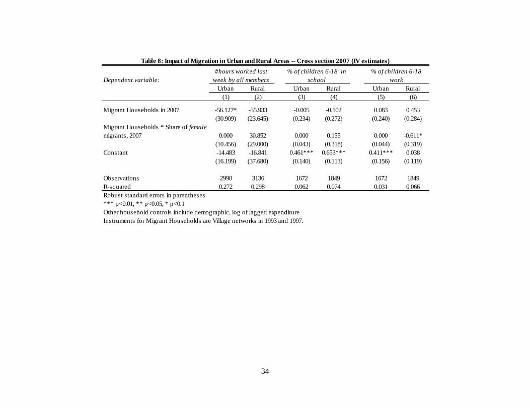
34

Dependent variable:

Urban Rural Urban Rural Urban Rural

(1) (2) (3) (4) (5) (6)

Migrant Households in 2007 -56.127* -35.933 -0.005 -0.102 0.083 0.453

(30.909) (23.645) (0.234) (0.272) (0.240) (0.284)

Migrant Households * Share of female

migrants, 2007 0.000 30.852 0.000 0.155 0.000 -0.611*

(10.456) (29.000) (0.043) (0.318) (0.044) (0.319)

Constant -14.483 -16.841 0.461*** 0.653*** 0.411*** 0.038

(16.199) (37.680) (0.140) (0.113) (0.156) (0.119)

Observations 2990 3136 1672 1849 1672 1849

R-squared 0.272 0.298 0.062 0.074 0.031 0.066

Robust standard errors in parentheses

*** p<0.01, ** p<0.05, * p<0.1

Other household controls include demographic, log of lagged expenditure

Instruments for Migrant Households are Village networks in 1993 and 1997.

Table 8: Impact of Migration in Urban and Rural Areas -- Cross section 2007 (IV estimates)

#hours worked last

week by all members

% of children 6-18 in

school

% of children 6-18

work

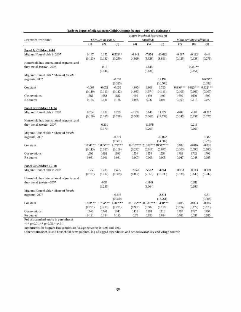
35

Dependent variable:

(1) (2) (3) (4) (5) (6) (7) (8) (9)

Panel A: Children 6-10

Migrant Households in 2007 0.147 0.152 0.503** -6.443 -7.854 -13.612 -0.087 -0.112 -0.44

(0.123) (0.132) (0.250) (4.929) (5.328) (8.811) (0.125) (0.133) (0.276)

Household has international migrants, and

they are all female --2007 -0.18 4.848 0.331**

(0.146) (5.634) (0.154)

Migrant Households * Share of female

migrants, 2007 -0.531 12.192 0.659**

(0.325) (10.506) (0.332)

Constant -0.064 -0.052 -0.055 4.035 3.808 3.755 0.846*** 0.825*** 0.832***

(0.110) (0.110) (0.112) (4.083) (4.074) (4.111) (0.106) (0.106) (0.107)

Observations 1682 1682 1682 1499 1499 1499 1699 1699 1699

R-squared 0.175 0.181 0.136 0.065 0.06 0.031 0.109 0.115 0.077

Panel B: Children 11-14

Migrant Households in 2007 0.204 0.182 0.289 -1.576 0.148 11.427 -0.09 -0.07 -0.212

(0.160) (0.165) (0.248) (9.368) (9.366) (12.532) (0.145) (0.151) (0.227)

Household has international migrants, and

they are all female --2007 -0.231 -11.578 0.218

(0.170) (9.299) (0.163)

Migrant Households * Share of female

migrants, 2007 -0.371 -21.872 0.382

(0.301) (14.502) (0.279)

Constant 1.034*** 1.085*** 1.077*** 18.267*** 20.318***18.517*** 0.032 -0.016 -0.001

(0.113) (0.107) (0.108) (6.272) (5.617) (5.677) (0.100) (0.096) (0.096)

Observations 1692 1692 1692 1554 1554 1554 1702 1702 1702

R-squared 0.081 0.091 0.081 0.007 0.003 0.005 0.047 0.048 0.035

Panel C: Children 15-18

Migrant Households in 2007 0.25 0.285 0.465 -7.041 -5.512 -4.864 -0.053 -0.113 -0.189

(0.181) (0.212) (0.339) (6.852) (7.355) (10.938) (0.130) (0.149) (0.242)

Household has international migrants, and

they are all female --2007 -0.33 -1.849 0.282

(0.235) (8.064) (0.186)

Migrant Households * Share of female

migrants, 2007 -0.516 -2.314 0.31

(0.390) (13.261) (0.308)

Constant 1.703*** 1.754*** 1.785*** 31.175*** 31.330***31.480*** 0.035 -0.003 -0.016

(0.221) (0.219) (0.221) (8.967) (8.982) (9.179) (0.174) (0.172) (0.173)

Observations 1740 1740 1740 1118 1118 1118 1797 1797 1797

R-squared 0.191 0.194 0.193 0.02 0.023 0.024 0.031 0.037 0.035

Robust standard errors in parentheses

*** p<0.01, ** p<0.05, * p<0.1

Instruments for Migrant Households are Village networks in 1993 and 1997.

Other controls: child and household demographics, log of lagged expenditure, and school availability and village controls

Enrolled in school

Hours in school last week (if

enrolled) Main activity is idleness

Table 9: Impact of Migration on Child Outcomes by Age -- 2007 (IV estimates)