impacts of nutrients on periphyton growth and periphyton-macroinvertebrates...

i

IMPACTS OF NUTRIENTS ON PERIPHYTON GROWTH AND PERIPHYTON-MACROINVERTEBRATES INTERACTIONS IN

SHALLOW LAKES: A MESOCOSM EXPERIMENT

A THESIS SUBMITTED TO

THE GRADUATE SCHOOL OF NATURAL AND APPLIED SCIENCES OF

MIDDLE EAST TECHNICAL UNIVERSITY

BY

NUR FİLİZ

IN PARTIAL FULFILLMENT OF THE REQUIREMENTS

FOR THE DEGREE OF MASTER OF SCIENCE

IN BIOLOGY

SEPTEMBER 2012

ii

Approval of the thesis:

IMPACTS OF NUTRIENTS ON PERIPHYTON GROWTH AND PERIPHYTON-

MACROINVERTEBRATES INTERACTIONS IN SHALLOW LAKES: A

MESOCOSM EXPERIMENT

submitted by NUR FİLİZ in partial fulfillment of the requirements for the

degree of Master of Science in Biology Department, Middle East

Technical University by,

Prof. Dr. Canan Özgen ______________

Dean, Graduate School of Natural and Applied Sciences

Prof. Dr. Musa Doğan ______________

Head of Department, Biology

Prof. Dr. Meryem Beklioğlu Yerli ______________

Supervisor, Biology Dept., METU

Examining Committee Members:

Assoc. Prof. Dr. Sertaç Önde _______________

Biology Dept., METU

Prof. Dr. Meryem Beklioğlu Yerli _______________

Biology Dept., METU

Prof. Dr. Ahmet Altındağ _______________

Biology Dept., Ankara University

Prof. Dr. Nilsun Demir _______________

Fisheries Engineering Dept., Ankara University

Assoc. Prof. Dr. Ayşegül Gözen _______________

Biology Dept., METU

Date: 14.09.2012

iii

I hereby declare that all information in this document has been

obtained and presented in accordance with academic rules and ethical

conduct. I also declare that, as required by these rules and conduct, I

have fully cited and referenced all material and results that are not

original to this work.

Name, Last Name : Nur Filiz

Signature :

iv

ABSTRACT

IMPACTS OF NUTRIENTS ON PERIPHYTON GROWTH AND

PERIPHYTON-MACROINVERTEBRATES INTERACTIONS IN

SHALLOW LAKES: A MESOCOSM EXPERIMENT

Filiz, Nur

M.Sc., Department of Biology

Supervisor : Prof. Dr. Meryem Beklioğlu Yerli

September 2012, 67 pages

Periphyton biomass on artificial strips was observed monthly to see the impacts

of nutrient differences on periphyton and periphyton-macroinvertebrates

interaction. The experiment was conducted for four months in a mesocosm

which were runned at six countries at the same time and with the same steps.

Eight enclosures at two meters depth were used that four of them had high

nutrient level and the other four had low nutrient level. Sediment, macrophyte,

fish, plankton, benthic invertebrates and water were added at the same time

and with the same way in all of the countries. Periphyton growth which formed

on artificial 32 cm2 strips for June, July, August and September were brushed to

filtered mesocosm water and dry mass, ash free dry mass, phosphorus content

and chlorophyl-a concentrations were measured. Grazer pressure on the

periphyton was observed with a laboratory experiment for July, August and

v

September months. At the end of the mesocosm experiment macrophytes and

fish were harvested. Macrophytes’ dry mass and fish’ abundance were

measured. Moreover at the end of the experiment epiphyton was also

measured. Three kajak cores were taken from sediment for macroinvertebrates

at the end of the experiment and identified. All physical features of mesocosm

enclosures and PVI data were recorded for every 2 weeks.

Periphyton biomass was higher concentrations in HN enclosures than LN tanks.

Only dry mass of periphyton biomass showed the opposite because of the marl

deposition in LN tanks. This finding was also reinforced by epiphyton samples

which was taken at the end of the experiment. LN enclosures had the more

abundance of macroinvertebrate. The groups we found in sediment which had

big grazer effect on periphyton such as gastropods and Chironomidae. Grazer

experiment showed that grazer effect on periphyton increased in time. Although

this raise, periphyton growth also increased in LN enclosures with nutrient

increasing. This may be indicate that nutrient effect has a stronger effect than

grazer pressure on periphyton.

As it is explained before in the beginning of the experiment all of the conditions

were the same except nutrient level. Thus, bottom-up effect changed the top-

down control and at the end of the experiment we saw the more periphyton

less macroinvertebrate and more fish in HN tanks while the opposite was seen

in LN tanks.

Keywords: periphyton, nutrient, grazing pressure, top-down bottom-up control,

mesocosm

vi

ÖZ

SIĞ GÖLLERDE BESİN TUZUNUN PERİFİTON VE PERİFİTON-

MAKROOMURGASIZ ETKİLEŞİMLERİ ÜZERİNE ETKİSİ: MEZOKOZM

DENEYİ

Filiz, Nur

Yüksek Lisans, Biyoloji Bölümü

Tez Yöneticisi : Prof. Dr. Meryem Beklioğlu Yerli

Eylül 2012, 67 sayfa

Bu çalışmada yapay substrat üzerindeki perifiton gelişimi besin tuzu

farklılıklarının perifiton gelişimi ve perifiton-makroomurgasız etkileşimi

üzerindeki etkisini görebilmek amacıyla incelendi. Deney aylık olarak dört ay

boyunca altı ülkede aynı anda başlayan ve aynı adımlarla devam eden bir

mezokozmda gerçekleştirildi. Deney için dört tanesi yüksek besin tuzuna geriye

kalan dört tanesi ise düşük besin tuzuna sahip iki metre derinliğindeki sekiz

adet tank kullanıldı. Dip çamuru, su içi bitkisi, balık, plankton, bentik

omurgasızları ve su her ülkede aynı zamanlarda aynı şekilde eklendi. Haziran,

Temmuz, Ağustos ve Eylül aylarında 32 cm2’lik yapay şeritler üzerinde oluşan

perifiton filtre edilmiş mezokozm suyuna fırçalanarak kuru ağırlık, organik

madde kuru ağırlığı, fosfor içeriği ve klorofil-a derişimi ölçüldü. Perifiton

üzerindeki avlanma baskısı Temmuz, Ağustos ve Eylül aylarında bir laboratuvar

deneyiyle gözlemlendi. Mezokozm deneyinin sonunda bitki ve balıklar toplandı.

Bitki kuru ağırlığı ve balık miktarı hesaplandı. Ayrıca deney sonunda epifiton

vii

miktarı da ölçüldü. Makroomurgasızlar için kajak koru ile üç adet çamur örneği

alındı ve sınıflandırma yapıldı. İki haftalık sürelerle tankların fiziksel özellikleri

kaydedildi ve PVI değerleri hesaplandı.

Perifiton miktarı yüksek besin tuzu derişimli tanklarda daha fazlaydı. Düşük

besin tuzu derişimli tanklarda meydana gelen marl oluşumu yüzünden sadece

perifiton kuru ağırlığı bunun tersi bir sonuç gösterdi. Bu bulgular deney sonunda

bitkiden alınan epifiton örnekleriyle de pekiştirildi. Makroomurgasızlar LN

tanklarında daha fazla miktarda bulundu. Gastropod ve Chironomidae gibi

bulduğumuz gruplar perifiton üzerinde oldukça fazla avlanma etkisine sahip

gruplardı. Laboratuvarda yapılan avlanma deneyi ise avlanmanın zaman

içerisinde arttığını gösterdi. Fakat bu artışa rağmen son ayda LN tanklarında

artan besin tuzu ile birlikte perifiton artışı görüldü. Bu belki de perifiton

üzerinde besin tuzu etkisinin avlanma etkisinden daha büyük olduğunu

göstermektedir.

Daha önce açıklandığı üzere deney başlangıcında besin tuzu miktarı hariç tüm

koşullar aynı idi. Başlangıçta aynı olan yukardan aşağı kontrol, besin tuzunun

aşağıdan yukarı etkisi ile deney sonunda değişmiştir ve HN tanklarda daha çok

balık, daha az omurgasız ve daha çok perifiton görürken, LN tanklarda tam

tersini gözlemledik.

Anahtar Kelimeler: perifiton, besin tuzu, otlanma baskısı, yukarıdan aşağıya

aşağıdan yukarıya kontrol, mezokozm

viii

To the 2 precious families;

First; Elfidan and Mehmet Filiz,

Second; Lab 204.

ix

ACKNOWLEDGMENTS

I would like to thank to my supervisor Prof. Dr. Meryem Beklioğlu Yerli for her

support, patience and understanding throughout my master study.

Special thanks to my lab friends for their valuable friendships Eti Levi, Gizem

Bezirci, Şeyda Erdoğan, Tuba Bucak, Arda Özen, Nihan Tavşanoğlu, Ayşe İdil

Çakıroğlu, Deniz Önal, Jan Coppens and former lab friend Ece Sarağlu.

I am really greatful for their great helps of maybe the sweetest girls in the

world Seval Özcan and Ümmühan Aslan from Denizli, Pamukkale University and

of course Gürçay Kıvanç Akyıldız for his guidance to me.

Statistically significant thanks goes to my real friend Sevgi Saraç who helped

me for statistic and answered my all questions patiently.

I would like to express my eternal gratitude to my family, especially

my parents, for everything.

Finally, I am thankful to TÜBİTAK for supporting my second year of master

study via Scholarship Programme for Postgraduate Study (2228) and Middle

East Technical University Scientific Research Projects Coordinatorship.

x

TABLE OF CONTENTS

ABSTRACT .............................................................................................. iv

ÖZ ......................................................................................................... iv

ACKNOWLEDGMENTS ............................................................................... ix

TABLE OF CONTENTS ................................................................................ x

LIST OF TABLES ..................................................................................... xiii

LIST OF FIGURES ................................................................................... xiv

LIST OF ABBREVATIONS ......................................................................... xvii

CHAPTERS

1. INTRODUCTION ......................................................................... 1

1.1 Shallow Lakes and Roles of Periphyton .................................... 1

1.2 Factors Affecting Periphyton .................................................. 5

1.2.1 Abiotic Factors .............................................................. 6

1.2.2 Biotic Factors ............................................................... 7

1.3 Aim of The Study ................................................................ 10

2. MATERIALS and METHODS ......................................................... 11

2.1 Mesocosm Experimental Design ........................................... 11

2.1.1 Study Site .................................................................. 16

2.1.2 Inoculums and Additions ............................................ 18

xi

2.1.3 Sampling ................................................................... 20

2.1.4 Laboratory Analyses .................................................... 20

2.2 Periphyton Experiment ........................................................ 21

2.2.1 Periphyton Experimental Design .................................. 22

2.2.2 Sampling ................................................................... 23

2.2.3 Laboratory analyses ................................................... 23

2.2.4 Grazer Experiment ...................................................... 24

2.3 Macrophyte and Macroinvertebrate Sampling and Analysis

Mesocosm Experimental Design ................................................. 27

2.4 Statistical Analyses............................................................. 28

3. RESULTS .................................................................................. 29

3.1 Physico-chemical Parameters ............................................. 29

3.2 Biological Parameters ........................................................ 35

3.2.1 Periphyton ................................................................. 35

3.2.1.1 Grazer Experiment .............................................. 38

3.2.2 Macrophytes .............................................................. 39

3.2.3. Macroinvertebrates ................................................... 42

4. DISCUSSION ............................................................................ 43

4.1 Physico-chemical Parameters ............................................. 43

4.2 Nutrient Effects ................................................................. 45

4.3 Macrophytes and Periphyton ............................................... 48

4.4 Macroinvertebrates and Periphyton ...................................... 51

4.5 Top-down, Bottom-up Effect ............................................... 53

xii

5. CONCLUSION ........................................................................................................ 55

REFERENCES ............................................................................................ 57

xiii

LIST OF TABLES

TABLES

Table 1.1 Pros and cons of various methods of periphyton biomass ................. 8

Table 2.1 Random distribution of the enclosures in the floating stage. ........... 14

Table 2.2 Lake selection criteria................................................................ 16

Table 2.3 Morphometric and hydrological characteristics of Dam Lake Yalıncak

............................................................................................................ 16

Table 2.4 Periphyton Strips Exposure Times ............................................... 23

Table 3.1 Mean value and standart deviation of phico-chemical parameters ... 34

Table 3.2 Mean value and standart errors of periphyton parameters ............ 37

Table 3.3 Mean value and standart error of macrophyte dry weight and

periphyton of macrophyte ........................................................................ 41

Table 3.4 Macroinvertebrates community of 3 kajak cores which was taken at

the end of the experiment from enclosures. ............................................... 42

xiv

LIST OF FIGURES

FIGURES

Figure 1.1 Alternative stable state .............................................................. 3

Figure 2.1 Joint countries to the mesocosm experiments in along an eastern

latitude gradient in Europe as part of a REFRESH project ............................. 12

Figure 2.2 Floating stage ......................................................................... 12

Figure 2.3 Before addition of the water to the tanks ................................... 14

Figure 2.4 After addition of water and sediment to the tanks ........................ 15

Figure 2.5 Different scenes of Dam Lake Yalıncak; a) a photo of the lake, b) the

bathymetry map of the lake, c) the contour map of the lake, d) Google Earth

scene of the lake .................................................................................... 17

Figure 2.6 Macrophyte and fish which were added to the enclosures; a)

Gasterosteus aculeatus, b) Myriophyllum spicatum .................................... 19

Figure 2.7 Strips before taking place in tanks. ............................................ 22

Figure 2.8 Grazer Experiment ................................................................... 26

Figure 3.1 Water levels of the enclosures during the experiment. ................. 30

Figure 3.2 Temperature degrees of the enclosures during the experiment ..... 30

Figure 3.3 Changes of secchi depth/water level ratio in high and low nutrient

level tanks in time. . ............................................................................... 30

Figure 3.4 Conductivity changes in time and with nutrient level. ................... 30

Figure 3.5 pH changes in time and with nutrient level. ................................ 31

xv

Figure 3.6 Changes of alkalinity in time and with nutrient level..................... 31

Figure 3.7 Dissolved oxygen change in time and with nutrient level. ............. 31

Figure 3.8 TP changes in time and with nutrient level. ................................. 33

Figure 3.9 SRP changes in time and with nutrient level.. .............................. 33

Figure 3.10 TN changes in time and nutrient level....................................... 33

Figure 3.11 Amonia changes in time and nutrient level. ............................... 33

Figure 3.12 Periphyton dry mass changings in time and with nutrient level. ... 36

Figure 3.13 Periphyton ash free dry mass changings in time and with nutrient

level...................................................................................................... 36

Figure 3.14 Periphyton TP changings in time and with nutrient level. ............. 36

Figure 3.15 Periphyton chlorophyll-a changings in time and with nutrient level.

............................................................................................................ 36

Figure 3.16 Changing of grazer pressure on periphyton .............................. 38

Figure 3.17 PVI% changings in time and with nutrient level. ........................ 39

Figure 3.18 Myriophyllum spicatum abundance in the HN and LN tanks at the

end of the experiment ............................................................................ 39

Figure 3.19 Chara contraria abundance in the HN and LN tanks at the end of

the experiment ...................................................................................... 39

Figure 3.20 Total plant abundance in the HN and LN tanks at the end of the

experiment ........................................................................................... 39

Figure 3.21 Chlorophyll-a concentrations of the periphyton on macrophyte. ... 40

Figure 4.1 Increasing the light intensity as a result decreasing of water level

above the periphyton strips with temperature. ........................................... 44

Figure 4.2 Marl development on the periphyton strips in LN tanks. ................ 46

Figure 4.3: a) PVI%, b) Periphyton chlorophyll-a concentrations, c) Periphyton AFDM, d)

Periphyton TP concentrations, e) Planktonic chlorophyll-a concentrations. ................ 50

xvi

Figure 4.4 Classical food web (Taken and adapted from Molles, 2010). .......... 50

Figure 4.5 The phosphorus concentrations of the tanks in the beginning of the

experiment ........................................................................................... 54

Figure 4.6 Fish abundance in HN and LN tanks at the end of the experiment. . 54

Figure 4.7 Macroinvertebrate abundance in HN and LN tanks at the end of the

experiment. ........................................................................................... 54

xvii

LIST OF ABBREVATIONS

AFDM Ash free dry mass

AM Ash mass

ANOVA Analysis of variance

ASS Alternative stable state

Chl-a Chlorophyll-a

DM Dry mass

DO Dissolved oxygen

HN High nutrient

LN Low nutrient

N Nitrogen

NH4 Amonia

NO3-NO2 Nitrite - Nitrate

P Phosphorus

PVI Plant volume inhabited

Rm-ANOVA Repeated measure of ANOVA

S/W Secchi disk depth/Water level

SRP Soleble reactive phosphorus

SS Suspended solids

TA Alkalinity

TDS Total dissolved solids

TN Total nitrogen

TP Total phosphorus

1

CHAPTER 1

INTRODUCTION

1.1 Shallow Lakes and Role of Periphyton

Although freshwaters consist a really small portion, approximately 0.01 %, of

the world water resources (Dudgeon et al., 2006; Wetzel, 2001), this tiny

portion has an essential role for all organisms via rich biodiversity and habitats

(Bailey et al., 2004; Naiman et al., 1995). Moreover freshwaters have

fundamental places in our lives in terms of providing us many goods, materials

and services. Lakes with rivers and wetlands are estimated to comprise over

25% of the total requirements of human societies and survival (Constanza et

al., 1997).

Considering the lakes in two main groups as shallow and deep, it is seen that

shallow lakes have not had the scientific attention until the second half of the

1980s as much as deep lakes. Deep lakes had the concentration of freshwater

ecology with their large basins containing a considerable volume of freshwater

and thermal stratification during summer (Wetzel, 2001; Meerhoff, 2010).

However almost 95% of world freshwater source is small (surface area <1 km)

and relatively shallow (mean depth <10 m) (Moss, 2010; Wetzel, 2001).

In contrast to deep lakes, shallow lakes have wider littoral zones with dense

submerged macrophytes and usually do not have thermal stratification

2

(Jeppesen et al., 1998). They have a larger littoral area for sediment-water

coupling which serve a rich habitat for organisms (Scheffer, 1998). Their depths

are sufficiently shallow to permit the light penetration from surface to the

bottom and reinforce photosynthesis of aquatic plants over the entire column

(Wetzel, 2001). Moreover they have a higher overall productivity of organisms

(Downing et al., 1990; Gasith and Hoyer, 1998).

Philips et al. (1978) revealed that nutrient amount changes linearly with turbid

water state and there is one possible community structure which is either

phytoplankton dominated clear water conditions or macrophyte dominated

turbid water conditions. However this hypothesis conflict with some

observations. Scheffer et al. (1993, 2001) showed that many ecosystems may

comprise more than one structures which are both phytoplankton dominated

turbid water state and macrophyte dominated clear water states and also

switches between those conditions based on stochastic events mediated by

some buffer mechanisms. These switchs named by alternative stable state

(ASS).

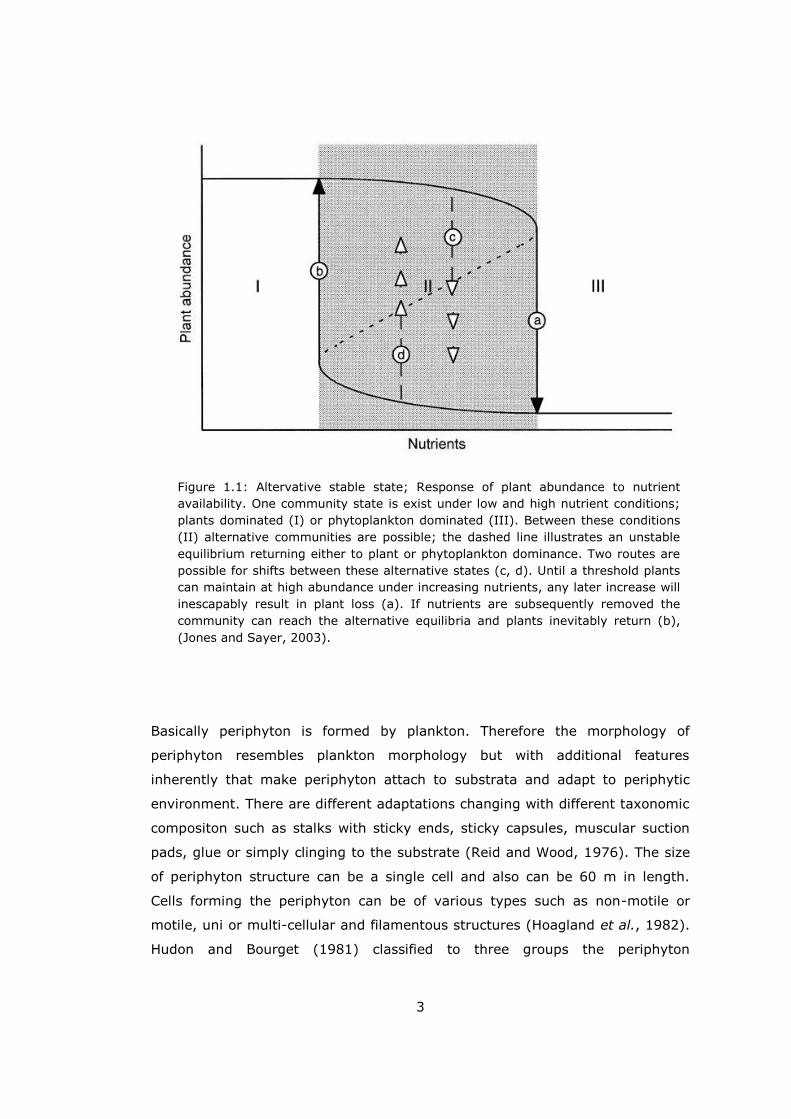
Figure 1.1 (Jones and Sayer 2003) showed the phytoplankton or macrophyte

dominated communities and the alternatives between them. Under low nutrient

conditions the lake will be macrophyte dominated, with increasing nutrients

plant loss may not be seen and this lead to the alternative equilibria. However

when the nutrient levels reach a threshold it will result with plant loss

eventually and lake will be phytoplankton dominated.

Periphyton refers to the entire community of sessile or fixed organisms on any

hard substrata (Azim et al., 2005). Van Dam et al., (2002) defined it as

composing of attached plant and animal organisms embedded in a

mucopolysaccharide matrix. ‘Attached algae’ or ‘attached microorganisms’ are

used by some authors as well however these terms are unsufficient to explain

the many other forms that lived on periphyton community. Moreover some

synonyms are used for periphyton based on the substrates (e.g epiphyton for

aquatic plant, epipelon for sediment, epixylon for wood etc., Azim et al., 2005;

Goldsborough, 2005) In this study, the term periphyton is used to refer to the

total complex of attached aquatic biota on plastic substrates.

3

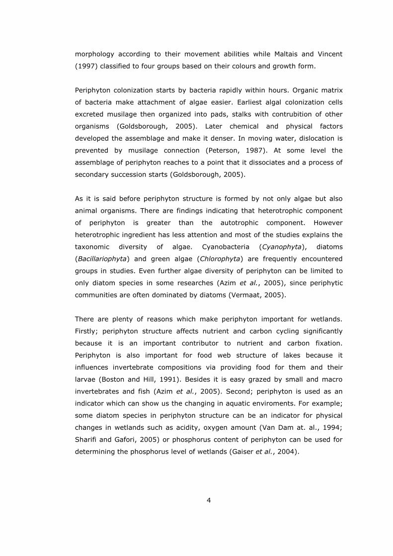
Basically periphyton is formed by plankton. Therefore the morphology of

periphyton resembles plankton morphology but with additional features

inherently that make periphyton attach to substrata and adapt to periphytic

environment. There are different adaptations changing with different taxonomic

compositon such as stalks with sticky ends, sticky capsules, muscular suction

pads, glue or simply clinging to the substrate (Reid and Wood, 1976). The size

of periphyton structure can be a single cell and also can be 60 m in length.

Cells forming the periphyton can be of various types such as non-motile or

motile, uni or multi-cellular and filamentous structures (Hoagland et al., 1982).

Hudon and Bourget (1981) classified to three groups the periphyton

Figure 1.1: Altervative stable state; Response of plant abundance to nutrient

availability. One community state is exist under low and high nutrient conditions;

plants dominated (I) or phytoplankton dominated (III). Between these conditions

(II) alternative communities are possible; the dashed line illustrates an unstable

equilibrium returning either to plant or phytoplankton dominance. Two routes are

possible for shifts between these alternative states (c, d). Until a threshold plants

can maintain at high abundance under increasing nutrients, any later increase will

inescapably result in plant loss (a). If nutrients are subsequently removed the

community can reach the alternative equilibria and plants inevitably return (b),

(Jones and Sayer, 2003).

4

morphology according to their movement abilities while Maltais and Vincent

(1997) classified to four groups based on their colours and growth form.

Periphyton colonization starts by bacteria rapidly within hours. Organic matrix

of bacteria make attachment of algae easier. Earliest algal colonization cells

excreted musilage then organized into pads, stalks with contrubition of other

organisms (Goldsborough, 2005). Later chemical and physical factors

developed the assemblage and make it denser. In moving water, dislocation is

prevented by musilage connection (Peterson, 1987). At some level the

assemblage of periphyton reaches to a point that it dissociates and a process of

secondary succession starts (Goldsborough, 2005).

As it is said before periphyton structure is formed by not only algae but also

animal organisms. There are findings indicating that heterotrophic component

of periphyton is greater than the autotrophic component. However

heterotrophic ingredient has less attention and most of the studies explains the

taxonomic diversity of algae. Cyanobacteria (Cyanophyta), diatoms

(Bacillariophyta) and green algae (Chlorophyta) are frequently encountered

groups in studies. Even further algae diversity of periphyton can be limited to

only diatom species in some researches (Azim et al., 2005), since periphytic

communities are often dominated by diatoms (Vermaat, 2005).

There are plenty of reasons which make periphyton important for wetlands.

Firstly; periphyton structure affects nutrient and carbon cycling significantly

because it is an important contributor to nutrient and carbon fixation.

Periphyton is also important for food web structure of lakes because it

influences invertebrate compositions via providing food for them and their

larvae (Boston and Hill, 1991). Besides it is easy grazed by small and macro

invertebrates and fish (Azim et al., 2005). Second; periphyton is used as an

indicator which can show us the changing in aquatic enviroments. For example;

some diatom species in periphyton structure can be an indicator for physical

changes in wetlands such as acidity, oxygen amount (Van Dam at. al., 1994;

Sharifi and Gafori, 2005) or phosphorus content of periphyton can be used for

determining the phosphorus level of wetlands (Gaiser et al., 2004).

5

Thirdly; periphyton is used for treating freshwaters and improve the water

quality (Azim et al., 2005). Milstein (2005) explains that introduction of hard

substrates to different habitats is resulted with periphyton development. This

enhances production of species and affects water quality. Periphyton is also

used for fish production management in fish ponds (e. g. van Dam et al., 2002;

van Dam and Verdegem, 2005; e. g. Azim 2004) or natural waters (Welcomme

R. L., 2005).

Lastly periphyton community contribute to primary production even as big as

phytoplankton do especially in lakes which are shallow and with large littoral

zones (Liboriussen and Jeppesen, 2003; Goldsborough and Robinson, 1996).

However it is generally taught that phytoplankton has the most important

portion for primary productivity. Researchs show that the significant and often

dominant contributers to the primary production are macrophytes and

periphyton (Loeb et al., 1983; Azim, 2001; Eminson ve Moss, 2007). Studies in

arctic, temperate and tropical regions show that periphyton is an important

contributor not only to primary production but also to higher trophic levels

(Hecky and Hesslein, 1995). Unfortunately there are not many studies on

perihyton-based food web (Lowe, 1996; Vadeboncoeur et al., 2002; Azim et al.,

2005) substantially the reason for that a number of methodological problems

(Goldsborough et al., 2005). According to Vadeboncoeur et al. (2002) from

91% of 193 studies measured only phytoplankton productivity, 4.5% measured

only periphyton productivity while 4.5% measured both of them. Moreover

there are wide studies on plant productivity but less is known about periphyton

effects to those systems (Goldsbourgh et al., 2005; Hecky and Hesslein, 1995).

1.2 Factors Affecting Periphyton

Abundance, diversity and productivity of periphytic community are affected by

several abiotic and biotic features. Understanding of the factors which

contribute to periphyton structure is critical for a full consideration of aquatic

ecosystem function. Here light, temperature, depth, water level and nutrient in

6

abiotic factors will take place and as biotic factors grazer effect and macrophyte

will be explained.

1.2.1 Abiotic Factors

Even though light had no important effect on abundance of periphyton,

different light intensities form different taxa in periphyton structure (Vermaat J.

E., 1995). For example if sufficient light is available, community will be

microalgae dominated. If there is light penetration, periphytic community will

be heterotroph dominated (Goldsborough, 1993). Although in very low light

regimes (12 µmol) periphytic growth is minimal (Hill and Fanta, 2008),

periphyton structure can support high irradiance (800 µmol) exposure

(Nofdianto, 2010). Photosynthesis occurs at levels far below maximum daily

irradiance and photoinhibition is typically rare (Goldsborough et al., 2005).

Temperature has effects on periphyton taxonomic structure like light regime

(Vermaat J. E., 2005). For example, while high temperatures make

Scenedesmus dominate, low temperatures favoured Navicula in Vermmat and

Hootsmans (1994)’ and Bothwell’s (1988) study. Besides it is same for season

differences that diatoms are dominant in spring and green algae or

cyanobacteria are dominant in summer (Meulemans and Roos, 1985).

Temperature and light often show strong parallelism because if there is

sunlight, it will provide light for phytosynthesis of macrophytes and warm up

the environment (Vermaat J. E., 2005). Therefore separation of temperature

and light interaction and impacts on periphyton growth is not very common

(Bothwell, 1988). Still there are some studies (Vermaat and Hootsmans, 1994;

Nofdianto, 2010) which showed the interaction of low temperature and high

irradiance or vice versa. Both of these studies determined the maximum growth

at 20°C and 200-225 µmol. This degree of temperature and light is optimum for

all organisms groups. Above or below these levels taxa and abundance is

changing.

7

Water level generally affects the periphyton structure because it affects the

light intensity directly and may cause turbidity indirectly by increasing the wind

impacts for wetlands (Goldsborough et al., 1995). Liboriussen and Jeppesen

(2006) studied the periphyton at different depths (0.1, 0.5, 0.9) and they did

not find a linear relationship between depth and periphyton abundance.

Nutrient effect on periphyton development has been studied many times

especially in streams (Vermaat, 2005). Biomass is the most used data for

periphyton growth among several methods (dry mass, ash free dry mass,

chlorophyll concentration, total phosphorus concentration and biovolume).

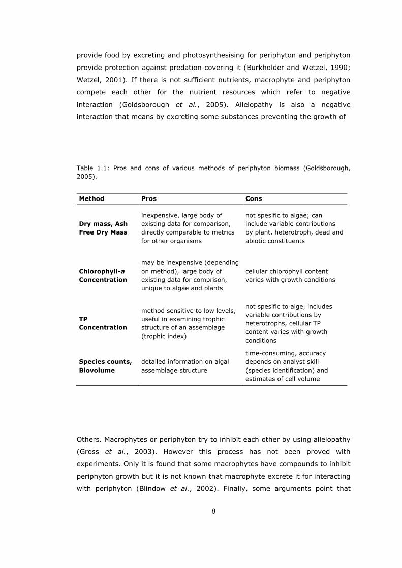
Goldsborough (2005) critisized the methods with their pros and cons (Table

1.1). These studies (Marcus, 1980; Hansson, 1992; Jones and Sayer, 2003;

Liboriussen et al., 2005, 2006; Smith and Lee, 2006; Becares et al., 2008;

Özkan et al., 2010; Rosemond et al., 1993, 2000; Chételat et al., 1999; Sharifi

and Ghafori, 2005; Greenwood and Rosemond, 2005; Bowes et al., 2010)

generally concluded that higher nutrient caused higher periphyton biomass in

both lakes and rivers.

Nutrient features of ecosystems, generally nitrogen and phosphorus, are also

determining the dominant algal taxa. For example like silicon for diatoms, some

goups need special requirements and some species can supply their need via

producing phosphatase (Kahlert and Pettersson, 2002) or nitrogenase

(Goldsborough et al., 2005) enzymes when the inorganic nutrients are scarse in

the environment.

1.2.2 Biotic Factors

Macrophyte and periphyton interaction is a unique relationship that has been

the focus of many studies in shallow lakes and wetlands. Their results can be

summarized to positive interactions (symbosis or mutualism), negative

interactions (competition and allelopathy) and no interaction (neutrality)

(Goldsborough et al., 2005). Symbosis interaction is explained as; macrophyte

8

provide food by excreting and photosynthesising for periphyton and periphyton

provide protection against predation covering it (Burkholder and Wetzel, 1990;

Wetzel, 2001). If there is not sufficient nutrients, macrophyte and periphyton

compete each other for the nutrient resources which refer to negative

interaction (Goldsborough et al., 2005). Allelopathy is also a negative

interaction that means by excreting some substances preventing the growth of

Table 1.1: Pros and cons of various methods of periphyton biomass (Goldsborough,

2005).

Method Pros Cons

Dry mass, Ash

Free Dry Mass

inexpensive, large body of

existing data for comparison,

directly comparable to metrics

for other organisms

not spesific to algae; can

include variable contributions

by plant, heterotroph, dead and

abiotic constituents

Chlorophyll-a

Concentration

may be inexpensive (depending

on method), large body of

existing data for comprison,

unique to algae and plants

cellular chlorophyll content

varies with growth conditions

TP

Concentration

method sensitive to low levels,

useful in examining trophic

structure of an assemblage

(trophic index)

not spesific to alge, includes

variable contributions by

heterotrophs, cellular TP

content varies with growth

conditions

Species counts,

Biovolume

detailed information on algal

assemblage structure

time-consuming, accuracy

depends on analyst skill

(species identification) and

estimates of cell volume

Others. Macrophytes or periphyton try to inhibit each other by using allelopathy

(Gross et al., 2003). However this process has not been proved with

experiments. Only it is found that some macrophytes have compounds to inhibit

periphyton growth but it is not known that macrophyte excrete it for interacting

with periphyton (Blindow et al., 2002). Finally, some arguments point that

9

macrophytes just have the surface periphyton need thus their relationship for

the most part is biologically neutral (Goldsborough et al., 2005).

Several researchers showing the interaction of macrophyte and periphyton

shading such as Neundorfer and Kemp (1993), Goldsborough et al. (2005),

Gross et al. (2003), Roberts et al. (2003), Phillips et al. (1978), and Köhler et

al. (2010) revealed that periphyton shading has a negative impact on

macrophyte abundance when nutrients increase in water. In these studies

water conditions were turbid, thus phytoplankton abundance and suspended

solids were also effective for the limitation of the light. Hillebrand and Kahlert

(2001) reported a linear relationship between periphyton and macrophyte.

While grazers are decreasing the periphyton biomass, they are increasing the

nutrient content of periphyton, significantly. This is caused with excreation of

nutrients, removal of older cells and finally more turbid water and plant loss.

Nevertheless it is accepted by some reseachers macrophyte may shade the

periphyton structure (Becares et al., 2008; Liboriussen and Jeppesen, 2003).

There are a broad variety of animals in freshwater which graze on periphyton.

The most important ones are gastropods, crustaceans, insect larvae and other

small size invertebrates (Vermaat, 2005; Jones et al., 2002). Besides

invertebrates, vertebrates can also feed on periphyton such as fish and

tadpoles. Grazers can be highly selective and like the other affecting factors

may alter the spatial pattern and structure of the periphyton community

(Vermaat, 2005). Hillebrand and Kahlert (2001) revealed that with nutrient

addition an increase occurs in grazer effects on periphyton composition.

Many studies (Mazumder et al., 1989; Liboriussen et al., 2003; Vadeboncoeur

et al., 2002; Jones and Sayer, 2003; Hillebrand, 2002) reported that

macroinvertebrates reduce periphyton biomass. Cattaneo and Mousseau (1995)

found that the most important impact on periphyton-macroinvertebrate

interaction is the grazer body size. Taxon of the grazer and the periphyton

algae composition are less important.

10

1.3 Aim of The Study

Periphyton growth has an important role in freshwater ecosystems and it is a

good indicator for changing conditions. Therefore it is crucial to understand its

interaction with biotic and abiotic factors in the shallow lakes. This study aimed

to reveal the relationships between nutrient and macroinvertebrates grazing

effects on periphyton. Also since this mesocosm study targeted to compare the

results with other countries which made the same experiment with the same

steps and which are at different latitudes, this study also aimed to provide data

for this comparison.

11

CHAPTER 2

MATERIALS and METHODS

2.1 Mesocosm Experimental Design

A mesocosm experiment was carried out in 6 EU-REFRESH participating

countries (Sweden, Estonia, Germany, the Czech Republic, Greece and Turkey)

at the same time with applying the same protocol to reveal the effects of water

level changes and nutrients on trophic structure, function and metabolisms in a

latitudinal gradient to show the relative importance of the benthic and pelagic

communities for production, respiration and nutrient dynamics in lakes (Figure

2.1).

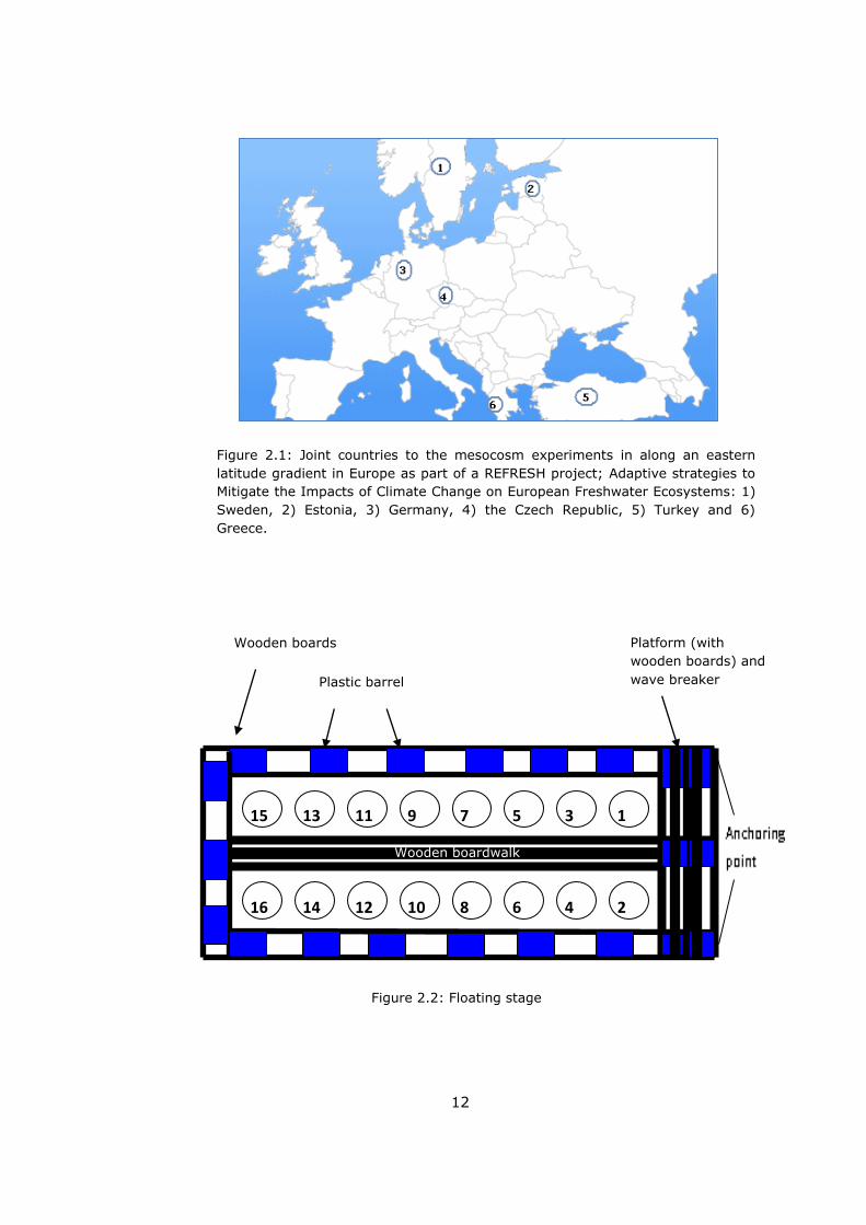
The experimental set-up was consisted of a floating stage (made of wooden

boards and floating devices like plastic barrels) which contained 16 enclosures

(two rows divided by a boardwalk). A platform and a boardwalk were built to

make working easier. Platform also took part as a wave breaker. The stage was

anchored from one side in order to limit its movement (Figure 2.2).

The enclosures were in cylindrical shape (R = 1.2 m), made of fibreglass (4

mm). Fibreglass is a strong material that prevents diffusion of O2 and CO2. The

enclosures were produced in İzmit, Turkey and were sent off the other

countries which were involved in the study.

12

Plastic barrel

Platform (with

wooden boards) and

wave breaker

Wooden boardwalk

Wooden boards

1 3 5 7 9 11 13 15

16 14 12 10 8 6 4 2

Figure 2.1: Joint countries to the mesocosm experiments in along an eastern

latitude gradient in Europe as part of a REFRESH project; Adaptive strategies to

Mitigate the Impacts of Climate Change on European Freshwater Ecosystems: 1)

Sweden, 2) Estonia, 3) Germany, 4) the Czech Republic, 5) Turkey and 6)

Greece.

Figure 2.2: Floating stage

13

Enclosures encompassed a 2x2x4 matrix (2 nutrients, 2 water levels, 4

replicates). Eight of them were 1.2 meters; four of these enclosures had high

(200 µg TP l-1) nutrient and the other four had low (25 µg TP l-1) nutrient level.

The other eight enclosures were 2.2 meters; similarly four of them had high

nutrient and the other four had low nutrient (Table 2.1).

The bottom of the tanks were covered by 10 cm lake sediment. The upper edge

of all tanks was attached to the stage 20 cm above the water surface in order

to provide a water depth in the 16 enclosures as 1 meter in shallows and 2

meters in high ones, respectively. A starting water volume (10 cm sediment, 90

cm water) was 1020 liters for 1.2 meters enclosures and (10 cm sediment, 190

cm water) was 2150 liters for 2,2 meters enclosures.

Ten percent (by volume) of the sediment that covered bottom of the enclosures

was oligotrophic local lake sediment and the remaining 90% was sand with a

grain size less than 1 mm. The local sediment was collected from 5 oligotrophic

lakes (Poyrazlar, Abant, Çubuk, İznik, Beyşehir) of Turkey. The collected mud

from five lakes was mixed, homogenised and sieved through a 10 mm mesh.

Large particles (>10 mm like plant fragments, mussels, stones etc.) were

removed.

Sediment was equilibrated to the desired nutrient level to adapt the mud to the

experimental conditions, enable easier creation and maintenance of phosphorus

(P) concentrations at two levels [25 (low tanks) and 250 (high tanks) µg TP l-1]

that took four months.

After establishment of placing the sediment to the tanks, enclosures were filled

with filtered (500 µm) lake water by the help of a water-pump. The date was

recorded as “day 0” and refered to May 9th 2011. To reduce the stirring of the

sediment a wooden disc was placed on top of the sediment during the addition

of water.

14

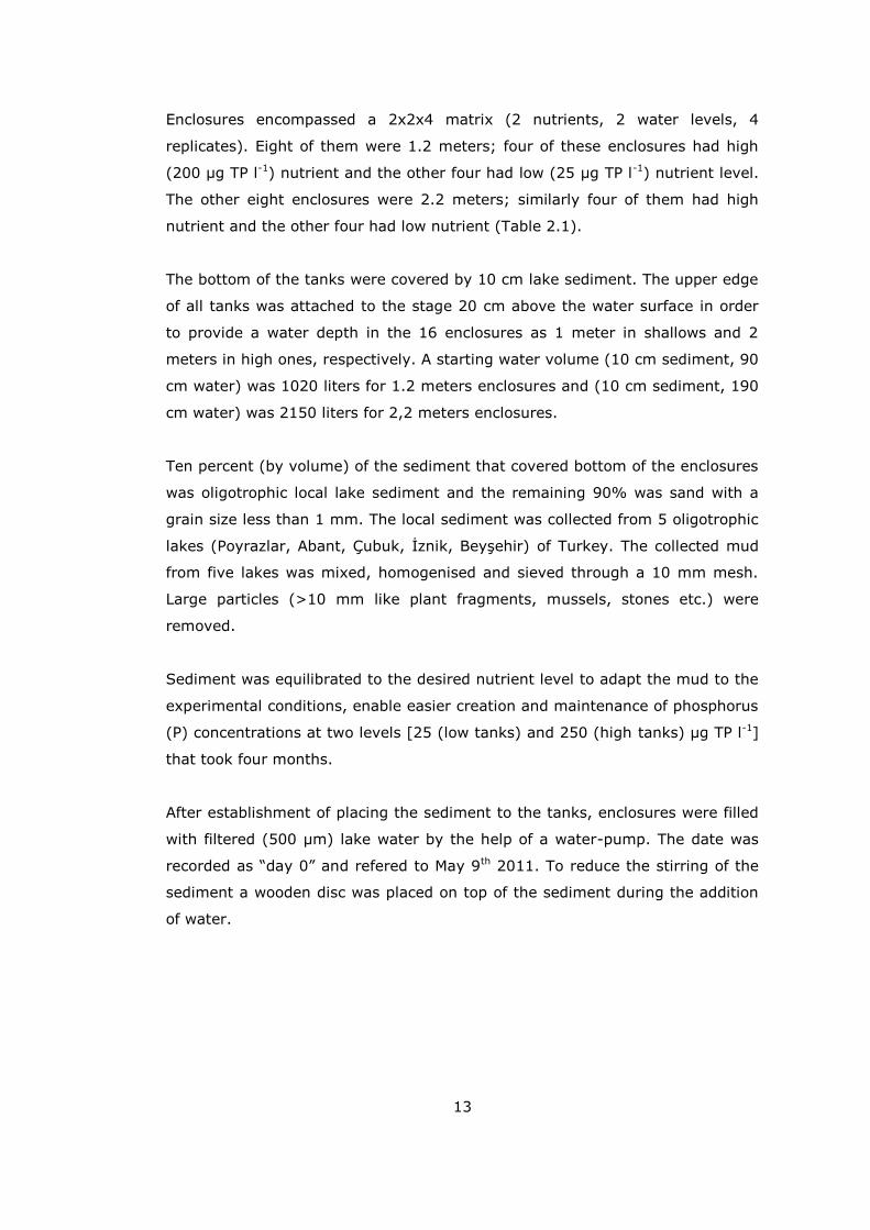
Table 2.1: Random distribution of the enclosures in the floating stage. Red ones were

used for the periphyton experiment and DH enclosures were labeled as high nutrient

(HN), DL enclosures were labeled low nutrient (LN). Shallow = 1 m, Deep = 2 m.

Enclosure number Depth Nutrient Enclosure name

1 Shallow High SH 1

2 Deep High DH 1 (HN 1)

3 Shallow High SH 2

4 Deep Low DL 1 (LN 1)

5 Shallow Low SL 1

6 Shallow High SH 3


8 Shallow Low SL 2

9 Shallow High SH 4


11 Shallow Low SL 3





16 Shallow Low SL 4

Figure 2.3: Before addition of the water to the tanks (METU limnology lab photo archive).

15

Stratification of the water column in the enclosures was avoided by water

pumps during the experiment. This process needed a continuous power suply.

Therefore a power cord from the shore was designed. Since there was no

electricity in study site exchangeable batteries were used as a power suply due

to make water pumps work and these batteries were changed every two or

three days, regularly. For circulation RS Electrical (RS-072A) 3 W filters were

used.

In addition a bird protecting net was used to prevent the birds to rest and

forage over the tanks.

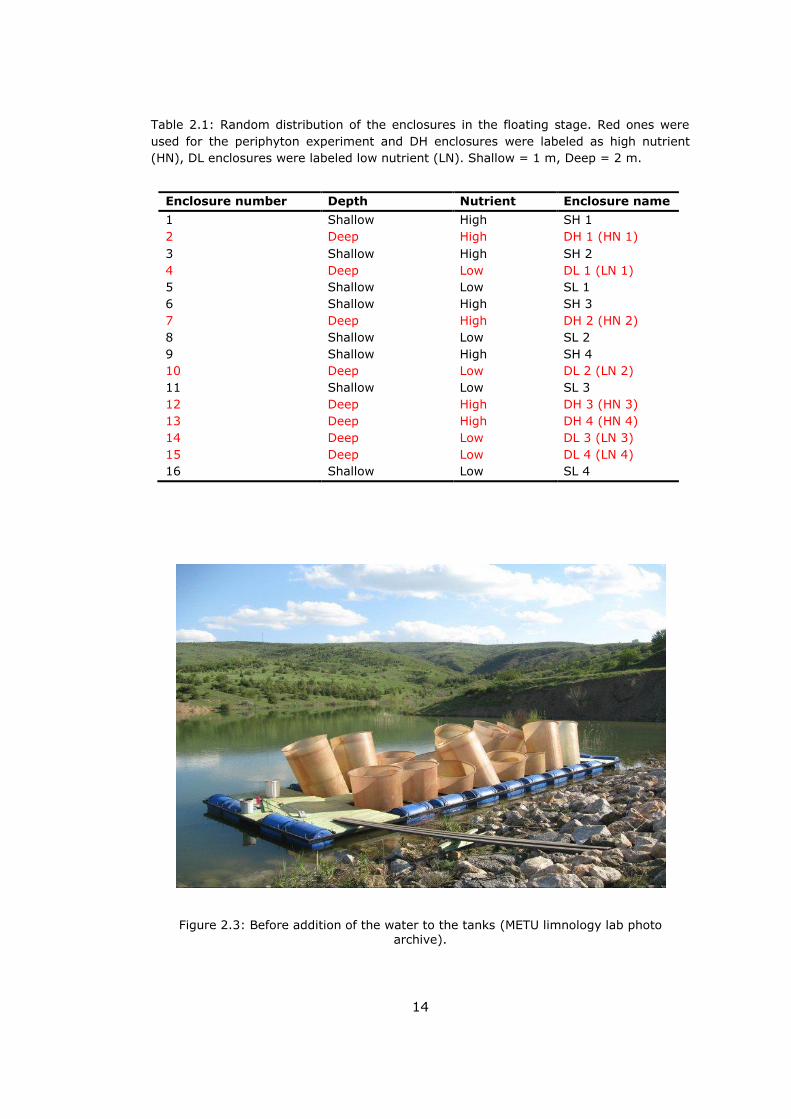
Figure 2.4: After addition of water and sediment to the tanks (METU limnology lab photo archive).

16

2.1.1 Study Site

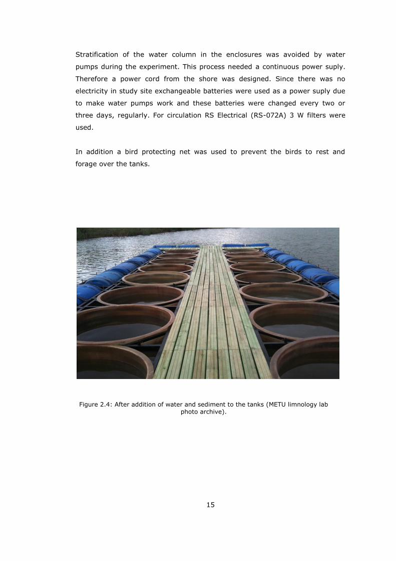
Yalıncak DSİ dam lake located at METU campus was selected for setting up

mesocosm experiment as it fullfilled some physical and chemical requirements

(Table 2.2) of the mesocosm experiment protocol according to which the

mesocosm experiments were set up and run in the 6 countries. Other

morphological and hydrological characterictics of the dam lake is summarized in

Table 2.3.

According to these conditions we selected Yalıncak Dam Lake which was made

by DSI in METU campus (39º52’N 32º46’ E, Figure 2.5). The closeness of the

lake to our department was also another reason for our choice. It’s building

started in 2002 however because of some financial problems ended in 2004. It

was made to prevent the flooding downstream and provide water for irrigation.

Table 2.2: Lake selection criteria.

Table 2.3: Morphometric and hydrological characteristics of Dam Lake Yalıncak.

Feature Values Feature Values

Area (ha) 1.96 TP (µg/l) 22.02

Max Depth (m) 11.3 Conductivity (µS/cm) 457.2

Oxygen (mg/l) 7.58 Secchi Depth (m) 168.75

TDS g/l 0.29 SRP (µg/l) 4.32

Chl-a µg/l 3.29 SS (mg) 3.34

pH 6.9

Feature Requested Values Dam Lake Yalıncak Values

Lake mean depth < 4 – 5 m 4.7 m

Lake alkalinity (TA) 1< TA < 4 meq/l 2.87 meq/l

Lake salinity < 1 ‰ 0.22 ‰

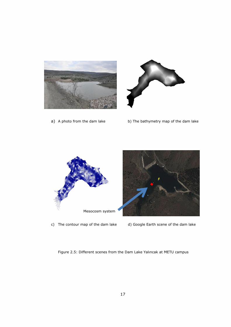
17

a) A photo from the dam lake b) The bathymetry map of the dam lake

c) The contour map of the dam lake d) Google Earth scene of the dam lake

Figure 2.5: Different scenes from the Dam Lake Yalıncak at METU campus

Mesocosm system

18

2.1.2 Inoculums and Additions

On the 4th day of the experiment (May 13rd 2011), in every countries, plankton

and a mixed sample of sediment collected from five other lakes (Poyrazlar,

Küçük Akgöl, Taşkısığı, Gölcük, Yeniçağ) were inoculated. They were collected

from these five lakes in order to enable potential development of a diverse flora

and fauna. Each of the five lakes was covering a nutrient gradient of 25 - 200

µg TP l-1. The sediment was collected from a low slope area and at a depth

corresponding to approximately mean depth of the lakes. In order to avoid fish

and large mussels sediment was filtered with a 10 mm mesh. The sediment was

mixed firmly and one litre of the inoculums sediment was added to each

enclosure by dispersing it evenly on top of the 10 cm sediment layer.

Zooplankton was collected from these five lakes through five vertical

zooplankton hauls covering the entire water column. Samples were kept

separately in 5 lt barrels filled with lake water from the sample lake. On the

addition day these five samples of plankton were mixed and a litre of the

plankton inoculated to each enclosure.

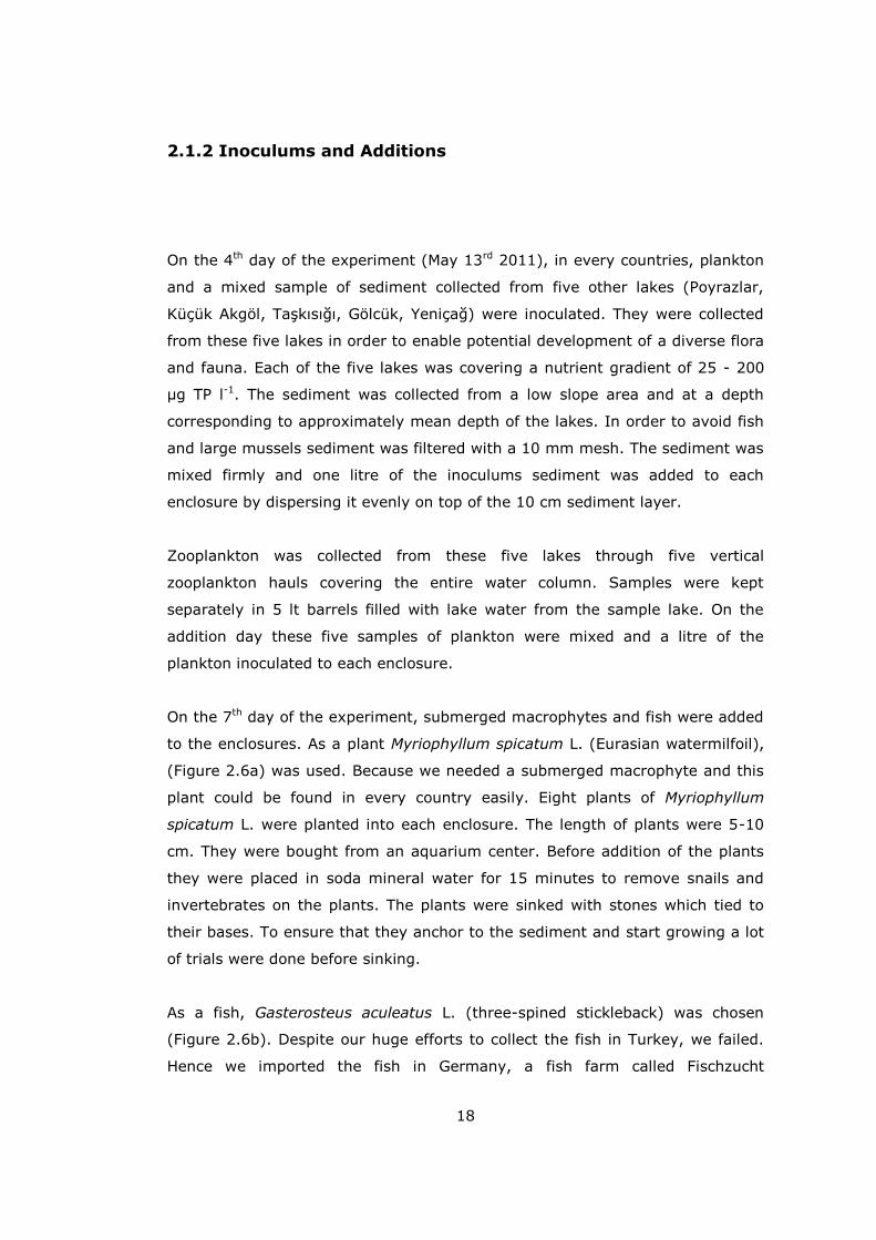
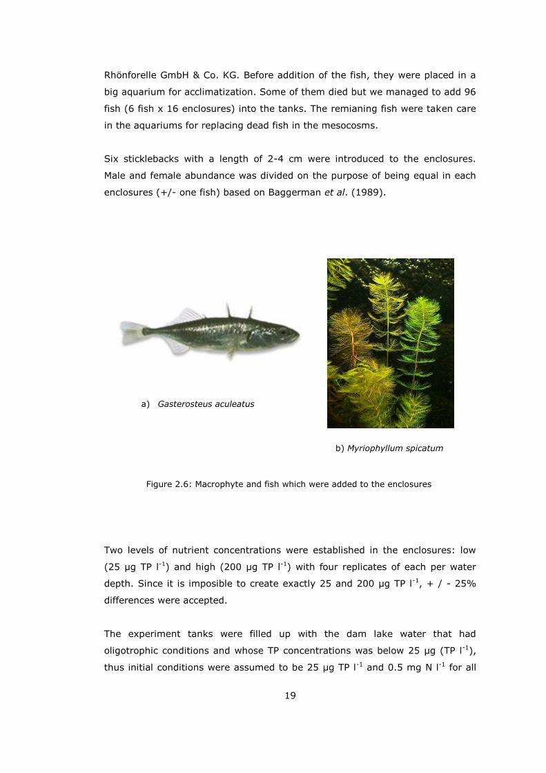
On the 7th day of the experiment, submerged macrophytes and fish were added

to the enclosures. As a plant Myriophyllum spicatum L. (Eurasian watermilfoil),

(Figure 2.6a) was used. Because we needed a submerged macrophyte and this

plant could be found in every country easily. Eight plants of Myriophyllum

spicatum L. were planted into each enclosure. The length of plants were 5-10

cm. They were bought from an aquarium center. Before addition of the plants

they were placed in soda mineral water for 15 minutes to remove snails and

invertebrates on the plants. The plants were sinked with stones which tied to

their bases. To ensure that they anchor to the sediment and start growing a lot

of trials were done before sinking.

As a fish, Gasterosteus aculeatus L. (three-spined stickleback) was chosen

(Figure 2.6b). Despite our huge efforts to collect the fish in Turkey, we failed.

Hence we imported the fish in Germany, a fish farm called Fischzucht

19

Rhönforelle GmbH & Co. KG. Before addition of the fish, they were placed in a

big aquarium for acclimatization. Some of them died but we managed to add 96

fish (6 fish x 16 enclosures) into the tanks. The remianing fish were taken care

in the aquariums for replacing dead fish in the mesocosms.

Six sticklebacks with a length of 2-4 cm were introduced to the enclosures.

Male and female abundance was divided on the purpose of being equal in each

enclosures (+/- one fish) based on Baggerman et al. (1989).

Figure 2.6: Macrophyte and fish which were added to the enclosures

Two levels of nutrient concentrations were established in the enclosures: low

(25 µg TP l-1) and high (200 µg TP l-1) with four replicates of each per water

depth. Since it is imposible to create exactly 25 and 200 µg TP l-1, + / - 25%

differences were accepted.

The experiment tanks were filled up with the dam lake water that had

oligotrophic conditions and whose TP concentrations was below 25 µg (TP l-1),

thus initial conditions were assumed to be 25 µg TP l-1 and 0.5 mg N l-1 for all

a) Gasterosteus aculeatus

b) Myriophyllum spicatum

20

tanks. So, there wasn’t any problem in the low nutrient enclosures but for the

high nutrient enclosures an initial addition was needed of both Phosphorus (P)

and Nitrogen (N) to provide the requirement of high TP and TN levels (200 µg

TP l-1, 2 mg N l-1). Since every country should have a standart for addition of

nutrients, eutrophic Danish Lakes were used as a base.

Moreover, because of the natural removal (like denitrification, sedimentation)

both N and P would decrease during the experiment. Hence, N and P were

added to all of the tanks every four weeks (+/- 2 days) in order to counteract

the natural removal and maintain the relative difference between low and high

nutrient levels in the enclosures. Na2HPO4 (4.60 g l-1) and Ca(NO3)2 (117.2 g l-1)

were used as P and N sources, respectively. The montly dosing of these

nutrients were carried out.

2.1.3 Sampling

Following the addition of fish and macrophytes the first sampling was made on

May 16th 2011. Thereafter we took samples from enclosures every two weeks. A

total of 2.75 lt were collected as 0.5 lt for water chemistry, 1.5 lt for chrophyl-

a, 0.5 lt for suspended solids, 0.25 lt for total nitrogen.

Temperature, dissolved oxygen, conductivity, total dissolved solids, salinity and

pH were measured by using YSI 556 MPS sensor from surface and 0.5 m

intervals through the water column monthly. In each sampling, water depth

and Secchi disc depth were recorded. Light also was measured at regular dates

by using LI-COR LI250A light meter.

21

2.1.4 Laboratory Analyses

Total phosphorus (TP), soluble reactive phosphorus (SRP) and alkalinity (TA)

were analysed on water chemistry samples. For determination of TP in water

sample, acid hydrolysis method was used (Mackereth et al., 1978). For SRP,

filtered water was processed with molybdate reaction method. TA analysis was

done with acid titration with phenolphtelene and BDH indicator (Mackereth et

al., 1978). Nitrogen analysis including total nitrogen (TN), ammonia (NH4) and

Nitrite-Nitrate (NO2,3) analysis were carried out using Scalar Autoanalyzer

Standart Methods (Houba et al., 1987; Krom, 1980; Kroon, 1993; Searle,

1984). Ethanol extraction method (Jespersen and Christoersen, 1987) was used

for determining the clorophyll-a with three replicates and measured at 663 and

750 nm spectrophotometer concentration.

2.2 Periphyton Experiment

In this mesocosm experiment, effects of nutrient levels on periphyton growth

was studied on an artificial substrate just in deep enclosures. As the water level

was assumed to have less effect in our set up, the artifical substrate periphyton

experiment was only carried out in the deep water enclosures. The tanks which

were deep and had the high nutrient level (DH) in the mesocosm experiment

will be hereafter regarded as high nutrient (HN) and the tanks which were deep

and had the low nutrient level (DL) will be regarded as low nutrient (LN).

22

2.2.1 Periphyton Experimental Design

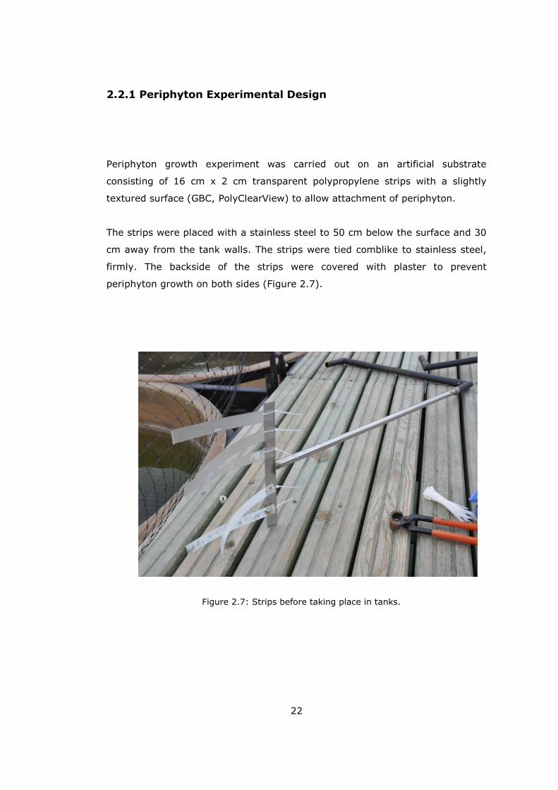
Periphyton growth experiment was carried out on an artificial substrate

consisting of 16 cm x 2 cm transparent polypropylene strips with a slightly

textured surface (GBC, PolyClearView) to allow attachment of periphyton.

The strips were placed with a stainless steel to 50 cm below the surface and 30

cm away from the tank walls. The strips were tied comblike to stainless steel,

firmly. The backside of the strips were covered with plaster to prevent

periphyton growth on both sides (Figure 2.7).

Figure 2.7: Strips before taking place in tanks.

23

2.2.2 Sampling

For four months periphyton strip samples were collected and strips were

changed with new ones monthly (Table 2.4).

Table 2.4: Periphyton Strips Exposure Times

1. month 18.06.2011 - 14.07.2011

2. month 15.07.2011 - 16.08.2011

3. month 16.08.2011 - 15.09.2011

4. month 16.09.2011 - 17.10.2011

After taking the strips out of the water, they were brushed with a toothbrush to

dislocate the sticky organisms into 150 ml filtered mesocosm water, mixed

firmly and taken to the laboratory for analyses.

2.2.3 Laboratory Analyses

The samples were used to determine of dry mass (DM), ash free dry mass

(AFDM), total phosphorus (TP) and chlorophyll-a (chl-a). Whatman 25 mm

GF/C filters were used to filter and analyse the suspension. Before the analyses

filters were always passed over pre-washed, pre-combusted, pre-weighed.

Firstly, 25 mg of suspension was filtered as two replicates then dried at 60ºC

overnight to determine dry mass (DM). Secondly, after measuring the DM filters

were combusted at 500ºC for 5 hours to determine ash mass (AM). After filters

24

were combusted, they placed in a desicator and waited for cooling off before

measuring the AM. AFDM was calculated by subtraction DM from AM (Roberts et

al. 2003).

For determination of total phosphorus (TP) in periphyton samples, acid

hydrolysis method was used (Mackereth et al., 1978). Since for this method 25

ml of sample is needed, 5 ml dense periphyton suspension diluted up to 25 ml

with distilled water and then analysed.

Lastly, 20 ml periphyton suspension with two replicates were filtered for

chlorophyl-a (chl-a) determination. Chl-a pigment content was determined with

ethanol extraction method (Jespersen and Christoersen, 1987) and the

absorbance was measured at 410, 430, 480, 663, 665 and 750 nm.

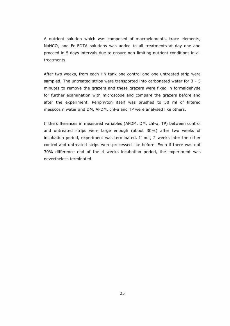
2.2.4 Grazer Experiment

A grazing laboratory experiment was also conducted to determine the effect of

invertebrate grazing pressure on periphyton biomass. Extra two strips (16 cm x

2 cm) were placed to high nutrient enclosures (HN) for the last three months of

the periphyton sampling (Table 2.4).

After these two strips were taken out of the mesocosms, they were cut into two

halves and transported to the lab immediately in a dark humid box. Thus there

were 4 piece (8 cm x 2 cm) of strips from each of HN enclosures (Figure 2.8).

In order to remove potential grazers which might have attached to the strips,

two strips from each enclosures were treated with CO2 for 3 - 5 minutes

(control strips). The other two were remained untreated. All strips were kept in

0.5 lt beakers under a light regime of 12 hours dark and 12 hours light and

constant temperature of 18ºC in the climate room. Throughout the incubation

of the strips the amount of water which was lost through evaporation was

replaced with filtered (Whatman GF/C filters) mesocosm water of the tank.

25

A nutrient solution which was composed of macroelements, trace elements,

NaHCO3 and Fe-EDTA solutions was added to all treatments at day one and

proceed in 5 days intervals due to ensure non-limiting nutrient conditions in all

treatments.

After two weeks, from each HN tank one control and one untreated strip were

sampled. The untreated strips were transported into carbonated water for 3 - 5

minutes to remove the grazers and these grazers were fixed in formaldehyde

for further examination with microscope and compare the grazers before and

after the experiment. Periphyton itself was brushed to 50 ml of filtered

mesocosm water and DM, AFDM, chl-a and TP were analysed like others.

If the differences in measured variables (AFDM, DM, chl-a, TP) between control

and untreated strips were large enough (about 30%) after two weeks of

incubation period, experiment was terminated. If not, 2 weeks later the other

control and untreated strips were processed like before. Even if there was not

30% difference end of the 4 weeks incubation period, the experiment was

nevertheless terminated.

26

Fig

ure

2.8

: G

razer

Experi

ment

27

2.3 Macrophyte and Macroinvertebrate Sampling and Analyses

On each sampling date and for each enclosure a species list was made for

macrophytes. Macrophyte percent plant volume inhabited (%PVI) was

calculated by visually estimating percentage coverage and measuring

macrophyte average plant height using the formula:

PVI = %coverage x average height / water depth (Canfield et al., 1984)

Coverage estimation was be performed by dividing the into quarters the

enclosures and estimating the area which covered by macrophyte by using the

scale:

0: no plants

1: 0-5% coverage

2: 5-25% coverage

3: 25-50% coverage

4: 25-75% coverage

5: 75-95% coverage

6: 95-100% coverage

If present, filamentous algae was included as part of the total macrophyte

coverage.

At the end of the experiment a piece of macrophyte were harvested from

enclosures in order to determine the periphyton content on the real plants. Dry

mass, ash free dry mass, cholorophyll-a and total phosphorus were measured.

Remaining of the macrophytes were all harvested, washed and dried at 105ºC

overnight to measure the dry weight of them.

For identification of macroinvertebrates three separate kajak cores were taken

from sediments of each enclosures at the end of the experiment. Samples are

pooled, rinsed, filtered on a 500 mm mesh and preserved in 96% ethanol. Their

identification was performed to familia level except Chironomidae. Since the

range of diversity was narrow and Chironomidae is a good indicator for nutrient

levels, Chironomidae familia was further identified to the species level with the

help from a specialist at the University of Pamukkale (Webb and Scholl 1985;

28

Şahin 1991; Epler, 2001 and Pilot and Vallenduk, 2002 keys were followed for

identification).

2.4 Statistical Analyses

SPSS 15.0 was used for all the statistics. Initial conditions tested with one-way

ANOVA to see if any difference existed among enclosures. Ln or sqrt

transformations were used to provide normality of data if necessary. Repeated

measure one-way ANOVA was used to see the changing nutrient and time

interaction. Bonferroni test was used to see the significant differences between

time periods. 95% confidence level was used for all statistical tests to show

statistical difference. For comparing the low and high nutrient level enclosures

of macrophyte dry weight, epiphyton parameters, macroinvertebrates and fish

abundance which was collected at the end of the experiment one way ANOVA

was used. Finally, linear regression analysis was used to see if there is any

important impact of physical conditions on periphyton biomass.

29

CHAPTER 3

RESULTS

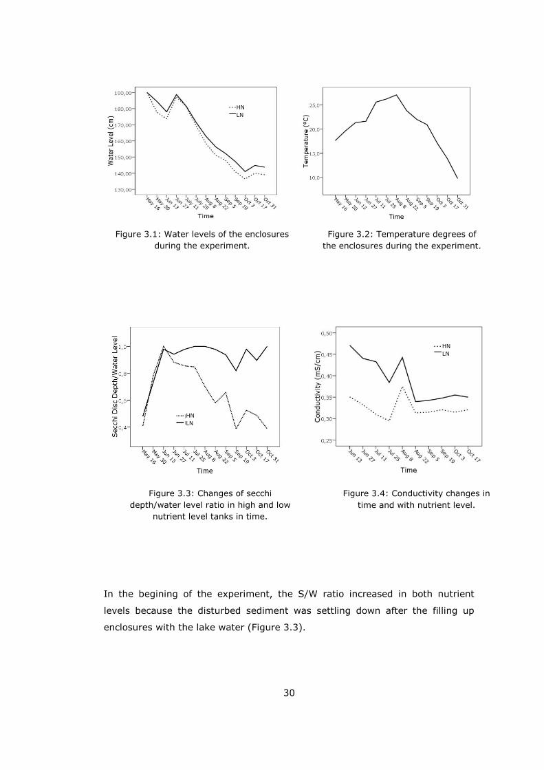
3.1 Physico-chemical Parameters

A major water level drop was observed for all of the enclosures throughout the

experiment. Only at the end of June water levels increased slightly because of

the precipitation. While water levels were 190 cm for all enclosures in the

begining, there were 0.51 ± 0.2 meter reduction in high nutrient level (HN) and

0.46 ± 0.1 meter reduction in low nutrient level (LN) enclosures at the end of

the experiment (Figure 3.1). A sharp decrease was observed after 11th July

when the enclosures’ water temparature reached to 25.57 ± 0.36 ºC. (Figure

3.2). Repeated measures of one-way ANOVA showed that there was not any

difference between HN and LN enclosures in terms of water temperature

(p=0.998) throughout the experiment (Table 3.1). In order to see how

temperature changing affected periphyton growth, linear regression analysis

was carried out. It showed that temperature did not have significant effect

neither on periphyton ash free dry mass, chlorophyll-a nor phosphorus amount.

Furthermore, stratification did not occur since we used water pumps to

stimulate mixing of water.

Secchi disc depth/water depth ratio (S/W) was used due to measure the clarity

of water which remained the same with the water depth in the LN tanks

whereas it significantly decreased through time in the HN ones (Table 3.1).

30

In the begining of the experiment, the S/W ratio increased in both nutrient

levels because the disturbed sediment was settling down after the filling up

enclosures with the lake water (Figure 3.3).

Figure 3.1: Water levels of the enclosures

during the experiment.

Figure 3.2: Temperature degrees of

the enclosures during the experiment.

Figure 3.3: Changes of secchi

depth/water level ratio in high and low

nutrient level tanks in time.

Figure 3.4: Conductivity changes in

time and with nutrient level.

HN

LN

HN

LN

HN

LN

31

One-way ANOVA was used if there was any difference between HN and LN

tanks for initial conditions. While water depth, temperature, Secchi disc

depth/water level ratio, pH, dissolved oxygen, nitrite-nitrate and amonnium

concentrations were no different initially; conductivity, alkalinity, total

Figure 3.5: pH changes in time and

with nutrient level.

Figure 3.6: Changes of alkalinity in

time and with nutrient level.

Figure 3.7: Dissolved oxygen change in time and with nutrient

level.

HN

LN

HN

LN

HN

LN

32

phosphorus, soluble reactive phosphorus and total nitrogen concentrations were

different for the beginning (Table 3.1).

Comparing the conductivity through all treatments repeated measure of ANOVA

(Rm-ANOVA) revealed that nutrient levels-time interaction was important on

conductivity (p<0.0001). It increased through time (p=0.001) and there were

significant differences between 4th (Jul 25) - 5th (Aug 8) and 5th - 6th (Aug 22)

samplings. Conductivity was higher in LN treatments than in HN tanks (Figure

3.4, Table 3.1).

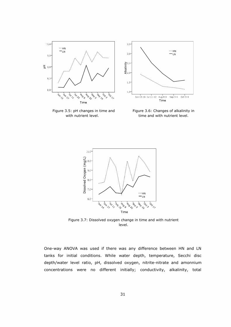
Rm-ANOVA showed that nutrient levels significantly affected pH, (p<0.0001).

pH of HN enclosures was greater than LN ones. Time also had important effect

on pH (p=0.007). It changed between 5th (Aug 8) - 6th (Aug 22) and 6th - 7th

(Sep 5) samplings (Figure 3.5, Table 3.1).

Rm-ANOVA indicated that alkalinity significantly changed with nutrient level and

time effect interaction (p=0.02). LN enclosures had higher alkalinity (Figure

3.6, Table 3.1).

Time and nutrient level interaction significantly affected (p<0.0001) dissolved

oxygen (DO). In the LN enclosures DO was lower than HN ones. However on 8th

August they were coming closer. 5th (Aug 8) and 6th (Aug 22) samplings were

different from each other, statistically (p=0.010, Figure 3.7, Table 3.1).

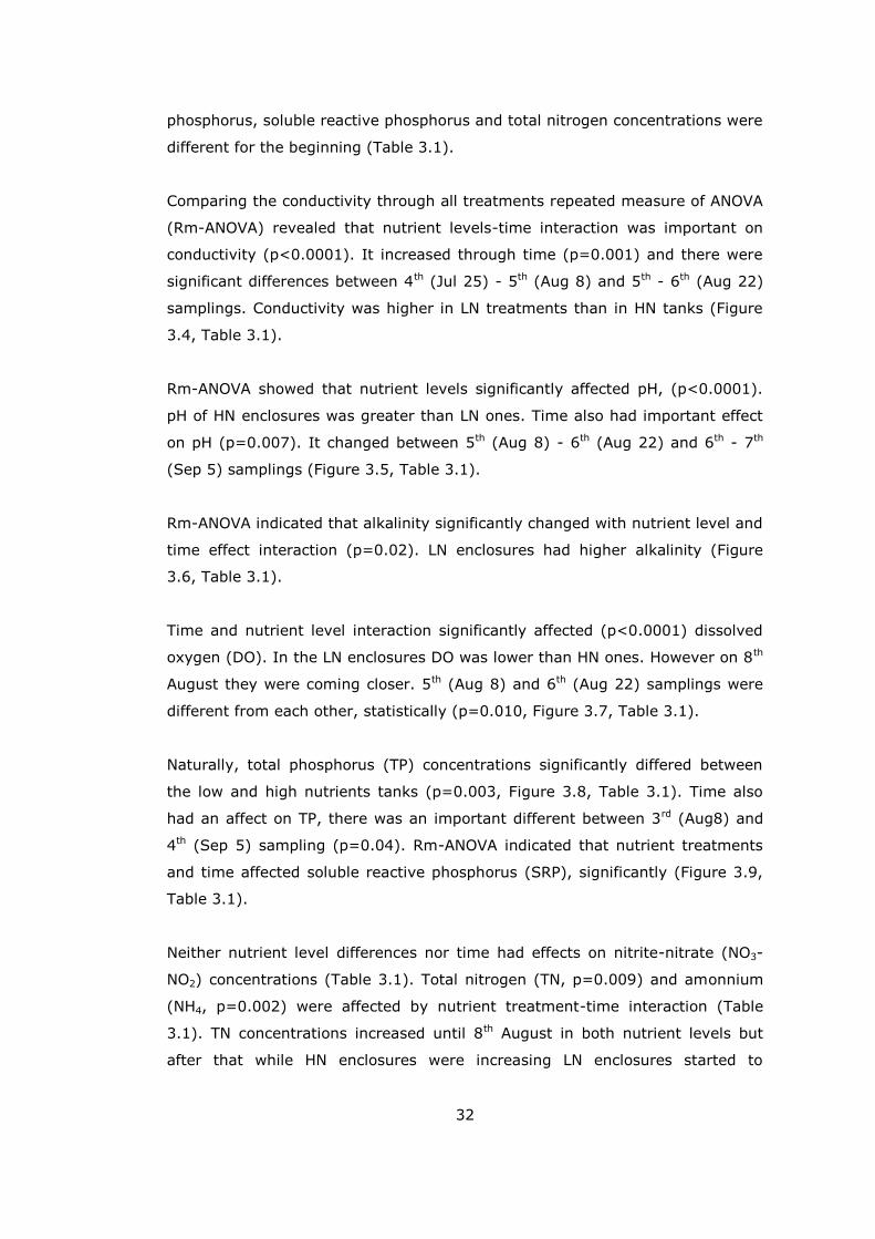
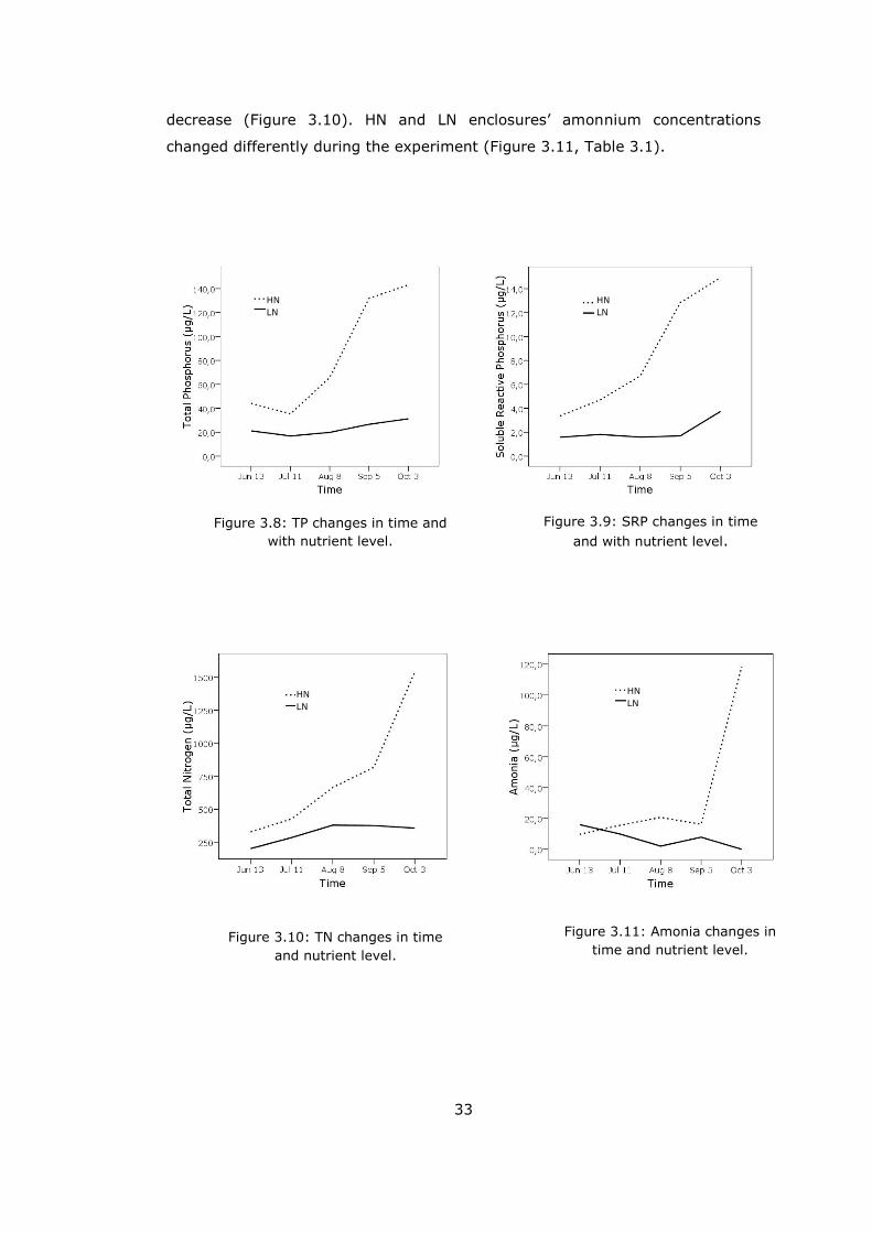
Naturally, total phosphorus (TP) concentrations significantly differed between

the low and high nutrients tanks (p=0.003, Figure 3.8, Table 3.1). Time also

had an affect on TP, there was an important different between 3rd (Aug8) and

4th (Sep 5) sampling (p=0.04). Rm-ANOVA indicated that nutrient treatments

and time affected soluble reactive phosphorus (SRP), significantly (Figure 3.9,

Table 3.1).

Neither nutrient level differences nor time had effects on nitrite-nitrate (NO3-

NO2) concentrations (Table 3.1). Total nitrogen (TN, p=0.009) and amonnium

(NH4, p=0.002) were affected by nutrient treatment-time interaction (Table

3.1). TN concentrations increased until 8th August in both nutrient levels but

after that while HN enclosures were increasing LN enclosures started to

33

decrease (Figure 3.10). HN and LN enclosures’ amonnium concentrations

changed differently during the experiment (Figure 3.11, Table 3.1).

Figure 3.9: SRP changes in time

and with nutrient level.

Figure 3.8: TP changes in time and

with nutrient level.

Figure 3.10: TN changes in time

and nutrient level.

Figure 3.11: Amonia changes in

time and nutrient level.

HN

LN

HN

LN

HN

LN HN

LN

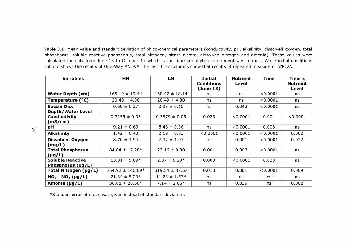
Table 3.1: Mean value and standart deviation of phico-chemical parameters (conductivity, pH, alkalinity, dissolved oxygen, total

phosphorus, soluble reactive phosphorus, total nitrogen, nitrite-nitrate, dissolved nitrogen and amonia). These values were

calculated for only from June 13 to October 17 which is the time periphyton experiment was runned. While initial conditions

column shows the results of One-Way ANOVA, the last three columns show that results of repeated measure of ANOVA.

*Standart error of mean was given instead of standart deviation.

Variables HN LN Initial

Conditions

(June 13)

Nutrient

Level

Time Time x

Nutrient

Level

Water Depth (cm) 165.19 ± 19.44 168.47 ± 18.14 ns ns <0.0001 ns

Temperature (ºC) 20.49 ± 4.86 20.49 ± 4.80 ns ns <0.0001 ns

Secchi Disc

Depth/Water Level

0.69 ± 0.27 0.95 ± 0.10 ns 0.043 <0.0001 ns

Conductivity

(mS/cm)

0.3255 ± 0.03 0.3879 ± 0.05 0.023 <0.0001 0.001 <0.0001

pH 9.21 ± 0.60 8.46 ± 0.36 ns <0.0001 0.008 ns

Alkalinity 1.42 ± 0.40 2.19 ± 0.73 <0.0001 <0.0001 <0.0001 0.002

Dissolved Oxygen

(mg/L)

8.70 ± 1.94 7.32 ± 1.07 ns 0.001 <0.0001 0.022

Total Phosphorus

(µg/L)

84.04 ± 17.28* 23.16 ± 9.30 0.001 0.003 <0.0001 ns

Soluble Reactive

Phosphorus (µg/L)

13.01 ± 5.09* 2.07 ± 0.29* 0.003 <0.0001 0.023 ns

Total Nitrogen (µg/L) 754.92 ± 140.69* 319.54 ± 87.57 0.010 0.001 <0.0001 0.009

NO3 - NO2 (µg/L) 21.34 ± 5.29* 11.23 ± 1.57* ns ns ns ns

Amonia (µg/L) 36.08 ± 20.66* 7.14 ± 2.05* ns 0.039 ns 0.002

35

3.2 Biological Parameters

3.2.1 Periphyton

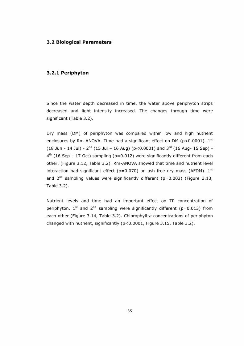
Since the water depth decreased in time, the water above periphyton strips

decreased and light intensity increased. The changes through time were

significant (Table 3.2).

Dry mass (DM) of periphyton was compared within low and high nutrient

enclosures by Rm-ANOVA. Time had a significant effect on DM (p<0.0001). 1st

(18 Jun - 14 Jul) - 2nd (15 Jul – 16 Aug) (p<0.0001) and 3rd (16 Aug- 15 Sep) -

4th (16 Sep – 17 Oct) sampling (p=0.012) were significantly different from each

other. (Figure 3.12, Table 3.2). Rm-ANOVA showed that time and nutrient level

interaction had significant effect (p=0.070) on ash free dry mass (AFDM). 1st

and 2nd sampling values were significantly different (p=0.002) (Figure 3.13,

Table 3.2).

Nutrient levels and time had an important effect on TP concentration of

periphyton. 1st and 2nd sampling were significantly different (p=0.013) from

each other (Figure 3.14, Table 3.2). Chlorophyll-a concentrations of periphyton

changed with nutrient, significantly (p<0.0001, Figure 3.15, Table 3.2).

36

Figure 3.12: Periphyton dry mass

changings in time and with nutrient

level.

Figure 3.13: Periphyton ash free dry

mass changings in time and with

nutrient level.

Figure 3.14: Periphyton TP changings

in time and with nutrient level.

Figure 3.15: Periphyton chlorophyll-a

changings in time and with nutrient

level.

HN

LN

HN

LN

HN

LN

HN

LN

HN

LN

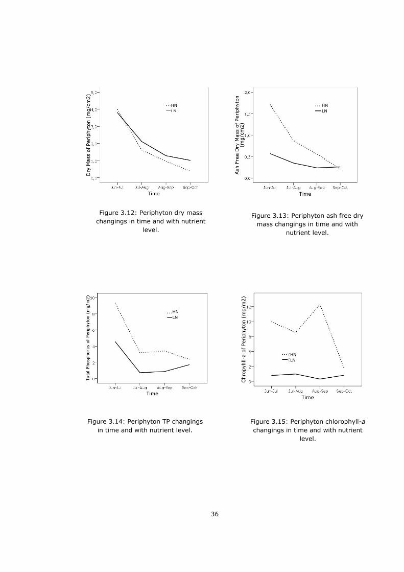
Table 3.2: Mean value and standart errors of periphyton parameters (dry mass, ash free dry mass, total phosphorus, chrophyll-

a, water levels above periphyton strips and light intensity) and PVI%. The last three columns showed the results of Rm-ANOVA.

Variables HN LN Nutrient Level Time Time x

Nutrient Level

Water Levels Above Periphyton

Strips

20.48 ± 2.92 23.46 ± 2.76 ns <0.0001 ns

Light Intensity Above Periphyton

Strips

983.9 ± 104.5 883.6 ± 75.7 ns <0.0001 ns

Dry Mass of Periphyton (mg/cm2) 1.74 ± 0.22 2.06 ± 0.29 ns <0.0001 ns

Ash Free Dry Mass of Periphyton

(mg/cm2)

0.84 ± 0.15 0.35 ± 0.05 0.015 <0.0001 0.007

Total Phosphorus of Periphyton

(mg/m2)

4.59 ± 1.12 1.97 ± 0.65 0.041 0.002 ns

Chrophyll-a of Periphyton (mg/m2) 8.47 ± 2.32 0.95 ± 0.18 <0.0001 0.046 ns

PVI% 25.29 ± 5.6 8.40 ± 1.29 0.010 <0.0001 0.005

38

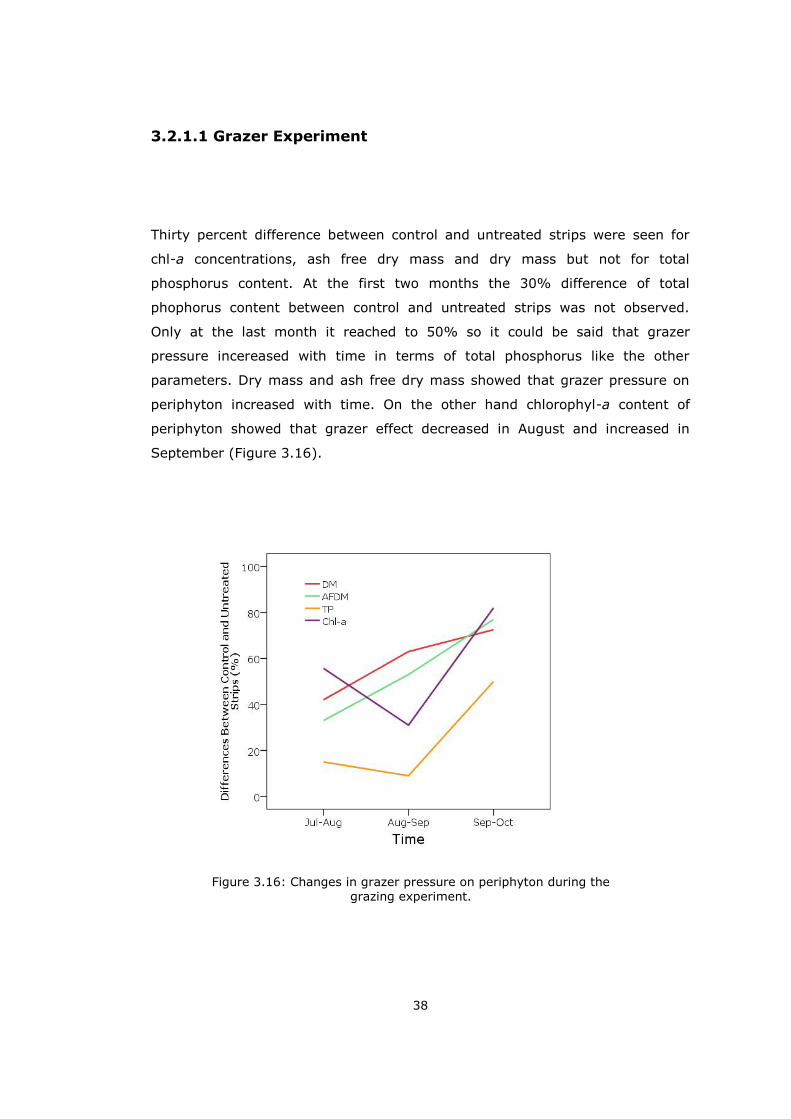
3.2.1.1 Grazer Experiment

Thirty percent difference between control and untreated strips were seen for

chl-a concentrations, ash free dry mass and dry mass but not for total

phosphorus content. At the first two months the 30% difference of total

phophorus content between control and untreated strips was not observed.

Only at the last month it reached to 50% so it could be said that grazer

pressure incereased with time in terms of total phosphorus like the other

parameters. Dry mass and ash free dry mass showed that grazer pressure on

periphyton increased with time. On the other hand chlorophyl-a content of

periphyton showed that grazer effect decreased in August and increased in

September (Figure 3.16).

Figure 3.16: Changes in grazer pressure on periphyton during the grazing experiment.

39

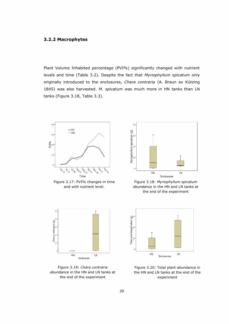
3.2.2 Macrophytes

Plant Volume Inhabited percentage (PVI%) significantly changed with nutrient

levels and time (Table 3.2). Despite the fact that Myriophyllum spicatum only

originally introduced to the enclosures, Chara contraria (A. Braun ex Kützing

1845) was also harvested. M. spicatum was much more in HN tanks than LN

tanks (Figure 3.18, Table 3.3).

Figure 3.17: PVI% changes in time

and with nutrient level.

Figure 3.18: Myriophyllum spicatum

abundance in the HN and LN tanks at

the end of the experiment

Figure 3.19: Chara contraria

abundance in the HN and LN tanks at

the end of the experiment

Figure 3.20: Total plant abundance in

the HN and LN tanks at the end of the

experiment

LN

HN

HN LN

HN HN

LN LN

40

None of the HN enclosures had C. contraria while LN tanks had considerable

amount which provided that LN enclosures had much more macrophyte at total

(Figure 3.19 and 3.20, Table 3.3). However PVI% graph showed us HN

enclosures had higher PVI% value. Since C. contraria was at the bottom of the

tanks they did not reflected the PVI% (Figure 3.17). The 4th high nutrient

enclosure (DH4 or HN4) had neither macrophyte nor filamenteous algae at the

end of the experiment.

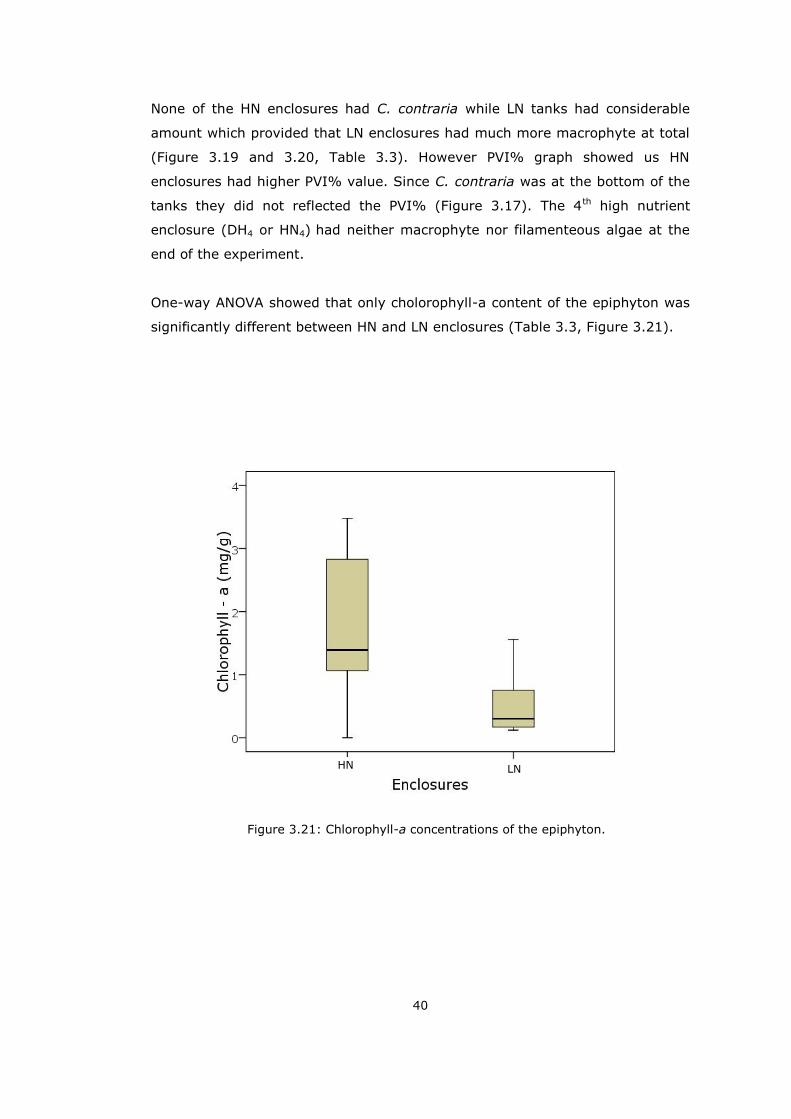
One-way ANOVA showed that only cholorophyll-a content of the epiphyton was

significantly different between HN and LN enclosures (Table 3.3, Figure 3.21).

Figure 3.21: Chlorophyll-a concentrations of the epiphyton.

HN LN

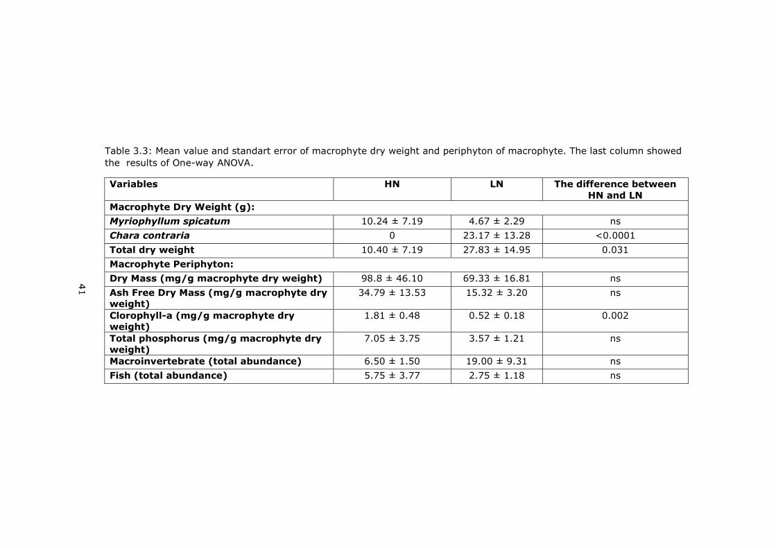
Table 3.3: Mean value and standart error of macrophyte dry weight and periphyton of macrophyte. The last column showed

the results of One-way ANOVA.

Variables HN LN The difference between

HN and LN

Macrophyte Dry Weight (g):

Myriophyllum spicatum 10.24 ± 7.19 4.67 ± 2.29 ns

Chara contraria 0 23.17 ± 13.28 <0.0001

Total dry weight 10.40 ± 7.19 27.83 ± 14.95 0.031

Macrophyte Periphyton:

Dry Mass (mg/g macrophyte dry weight) 98.8 ± 46.10 69.33 ± 16.81 ns

Ash Free Dry Mass (mg/g macrophyte dry

weight)

34.79 ± 13.53 15.32 ± 3.20 ns

Clorophyll-a (mg/g macrophyte dry

weight)

1.81 ± 0.48 0.52 ± 0.18 0.002

Total phosphorus (mg/g macrophyte dry

weight)

7.05 ± 3.75 3.57 ± 1.21 ns

Macroinvertebrate (total abundance) 6.50 ± 1.50 19.00 ± 9.31 ns

Fish (total abundance) 5.75 ± 3.77 2.75 ± 1.18 ns

42

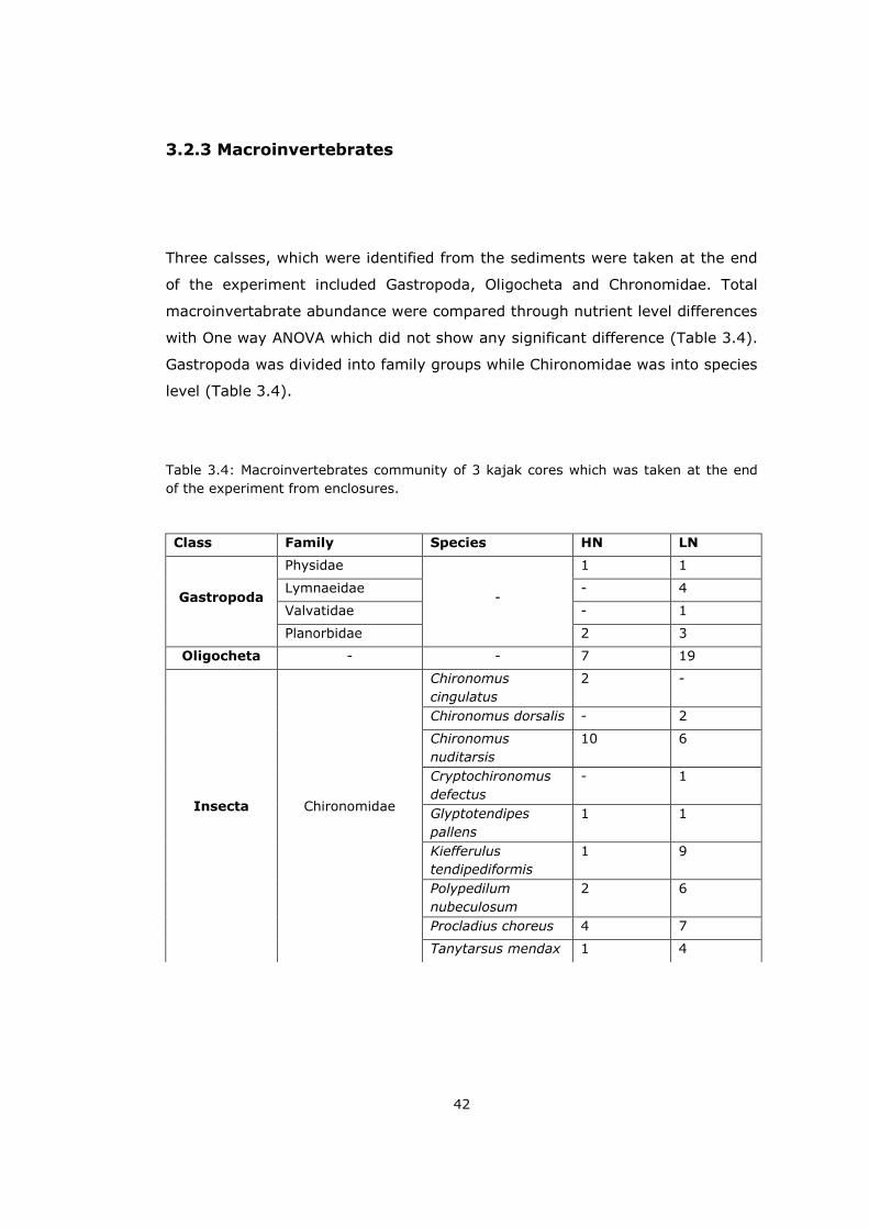
3.2.3 Macroinvertebrates

Three calsses, which were identified from the sediments were taken at the end

of the experiment included Gastropoda, Oligocheta and Chronomidae. Total

macroinvertabrate abundance were compared through nutrient level differences

with One way ANOVA which did not show any significant difference (Table 3.4).

Gastropoda was divided into family groups while Chironomidae was into species

level (Table 3.4).

Table 3.4: Macroinvertebrates community of 3 kajak cores which was taken at the end

of the experiment from enclosures.

Class Family Species HN LN

Gastropoda

Physidae

-

1 1

Lymnaeidae - 4

Valvatidae - 1

Planorbidae 2 3

Oligocheta - - 7 19

Insecta

Chironomidae

Chironomus

cingulatus

2 -

Chironomus dorsalis - 2

Chironomus

nuditarsis

10 6

Cryptochironomus

defectus

- 1

Glyptotendipes

pallens

1 1

Kiefferulus

tendipediformis

1 9

Polypedilum

nubeculosum

2 6

Procladius choreus 4 7

Tanytarsus mendax 1 4

43

CHAPTER 4

DISCUSSION

4.1 Physico-chemical Parameters

Water temperature of tanks changed significantly during experiment. Until 8th

August it increased ordinarily as considering the Mediterranean climate and the

maximum degree was observed at this date as 28ºC. In the end of the

September temperature decreased to approximately 20ºC. In present

experiment when periphyton strips were in tanks, temperature changed

between approximately 20 and 30ºC expect the last sampling (Sep 16 – Oct

17). It changed between approximately 20 - 13ºC (Table 3.2). Vermaat and

Hootsmans’ (1994) experiment showed that periphyton development changed

at three different temperatures (10, 15, 20 ºC), since temperature affects

enzymatic processes of periphyton community. At all these three level

periphyton growth increased but at 20ºC it reached to the carrying capacity in a

shorter time (30 days). According to DeNicola (1996) approximately a

temperature range of 0-30ºC increased the biomass of periphyton and 30-40ºC

decreased it. However, the temperatures that we observed in the current

experiment was most of the time above the critical temperature of their

experiment probably because of this we did not have major effect of

temperature on periphyton. Moreover linear regression analysis showed that

temperature did not have any significant effect on periphyton growth.

44

Usually temperature did not limit biomass in natural communities but it caused

an upper limit for production when other factors were optimal. If they were not,

primary productivity was limited by factors such as light, nutrients and grazing

depends on temperature (DeNicola, 1996).

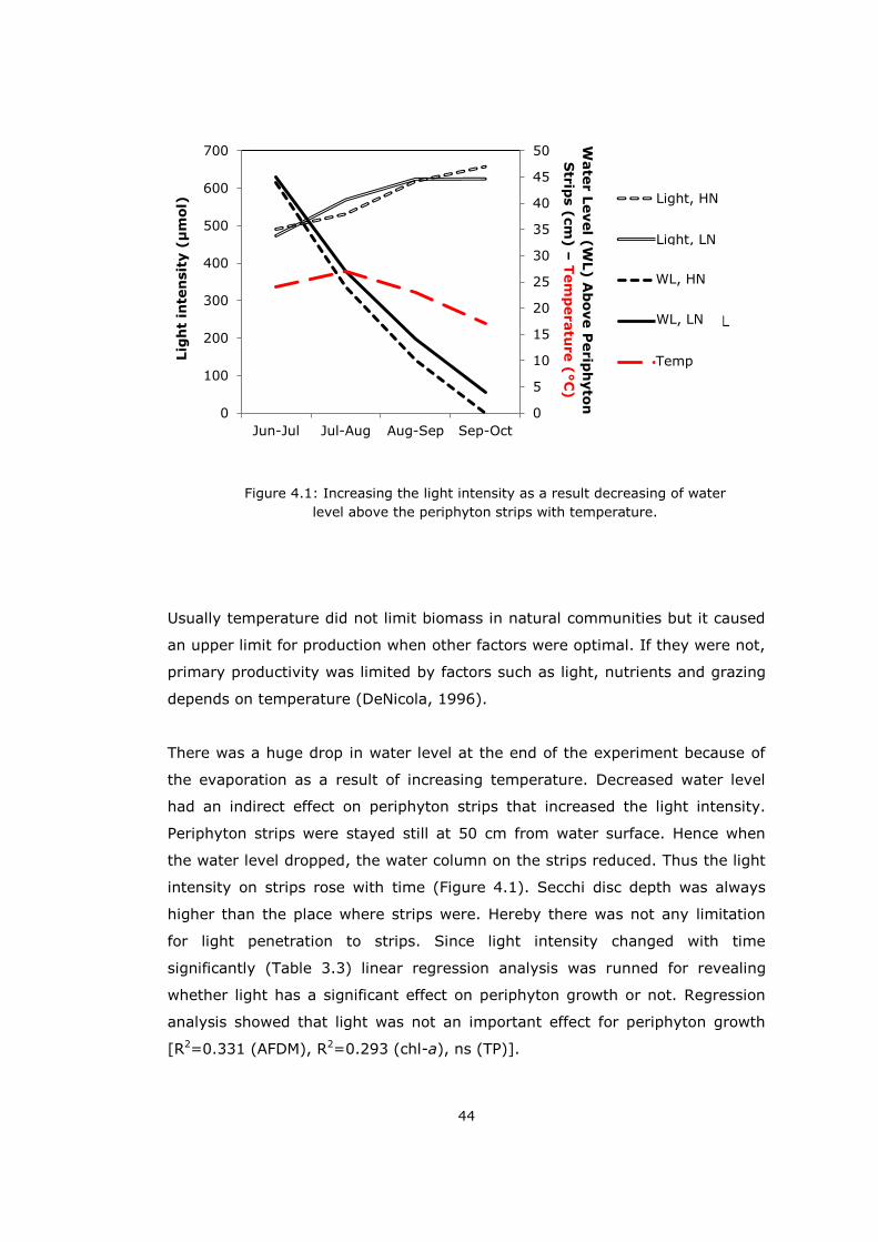
There was a huge drop in water level at the end of the experiment because of

the evaporation as a result of increasing temperature. Decreased water level

had an indirect effect on periphyton strips that increased the light intensity.

Periphyton strips were stayed still at 50 cm from water surface. Hence when

the water level dropped, the water column on the strips reduced. Thus the light

intensity on strips rose with time (Figure 4.1). Secchi disc depth was always

higher than the place where strips were. Hereby there was not any limitation

for light penetration to strips. Since light intensity changed with time

significantly (Table 3.3) linear regression analysis was runned for revealing

whether light has a significant effect on periphyton growth or not. Regression

analysis showed that light was not an important effect for periphyton growth

[R2=0.331 (AFDM), R2=0.293 (chl-a), ns (TP)].

0

5

10

15

20

25

30

35

40

45

50

0

100

200

300

400

500

600

700

Jun-Jul Jul-Aug Aug-Sep Sep-Oct

Light,DH

Light,DL

Depth,DH

Depth,DL

Temp

Figure 4.1: Increasing the light intensity as a result decreasing of water

level above the periphyton strips with temperature.

Lig

ht

inte

nsit

y (µ

mol)

Wate

r L

evel (

WL) A

bove P

erip

hyto

n

Str

ips (

cm

) –

Tem

peratu

re (°C

)

Light, HN

Light, LN

WL, HN

WL, LN

Temp

45

Light availability is a prior abiotic effect that high or low intensity of light causes

widely different taxa in periphyton structure and affects the dominant ones

(Loeb and Reuter, 1981). However, different light regimes had greatly similar

effects on growth curves and development of periphytic communities (Vermaat

and Hootsmans, 1994). Low light is sufficient for the periphyton community but

is also able to support high irradiance exposure (800 µmol; Nofdianto, 2010).

Only in very low level of light regime (15 µmol) periphytic algal development

will be minimal (Meulemans and Roos 1985; Liboriussen et al., 2005).

4.2 Nutrient Effects

Regarding the periphyton abundance on the strips; dry mass (DM), ash free dry

mass (AFDM), total phosphorus (TP) and chlorophyll-a (chl-a) content were

estimated. AFDM, chl-a and TP were greater in high nutrient level enclosures

(HN) than those of low ones (LN). On the other hand DM was greater in LN

tanks than HN tanks.

There are large number of researches showing the effects of nutrients on

periphyton which used chl-a parameter for periphyton biomass (Hansson, 1992;

Jones and Sayer, 2003; Liboriussen et al., 2005, 2006; Smith and Lee, 2006;

Becares et al., 2008; Özkan et al., 2010). Many of their results were similar

with the current experiment that chl-a content of periphyton was strongly

correlated with high nutrient levels in lakes. However Sánchez et al. (2010)

showed that periphyton chl-a amount was lower in the turbid lake (240 µg/L TP

and 1540 µg/L TN) than that of the clear lake (70 µg/L TP and 229 µg/L TN) in

Argentina. It was atributed to the light limitation imposed by planktonic

phytoplankton that took advantage of the nutrient availability in the water

column. Nevertheless, in our high nutrient enclosures light limitation was not

encountered for the periphyton strips because secchi disc depth were always

higher than 50 cm. Another experiment was concluded with an opposite result

is Hillebrand and Kahlert (2002) which was conducted for sediment periphyton

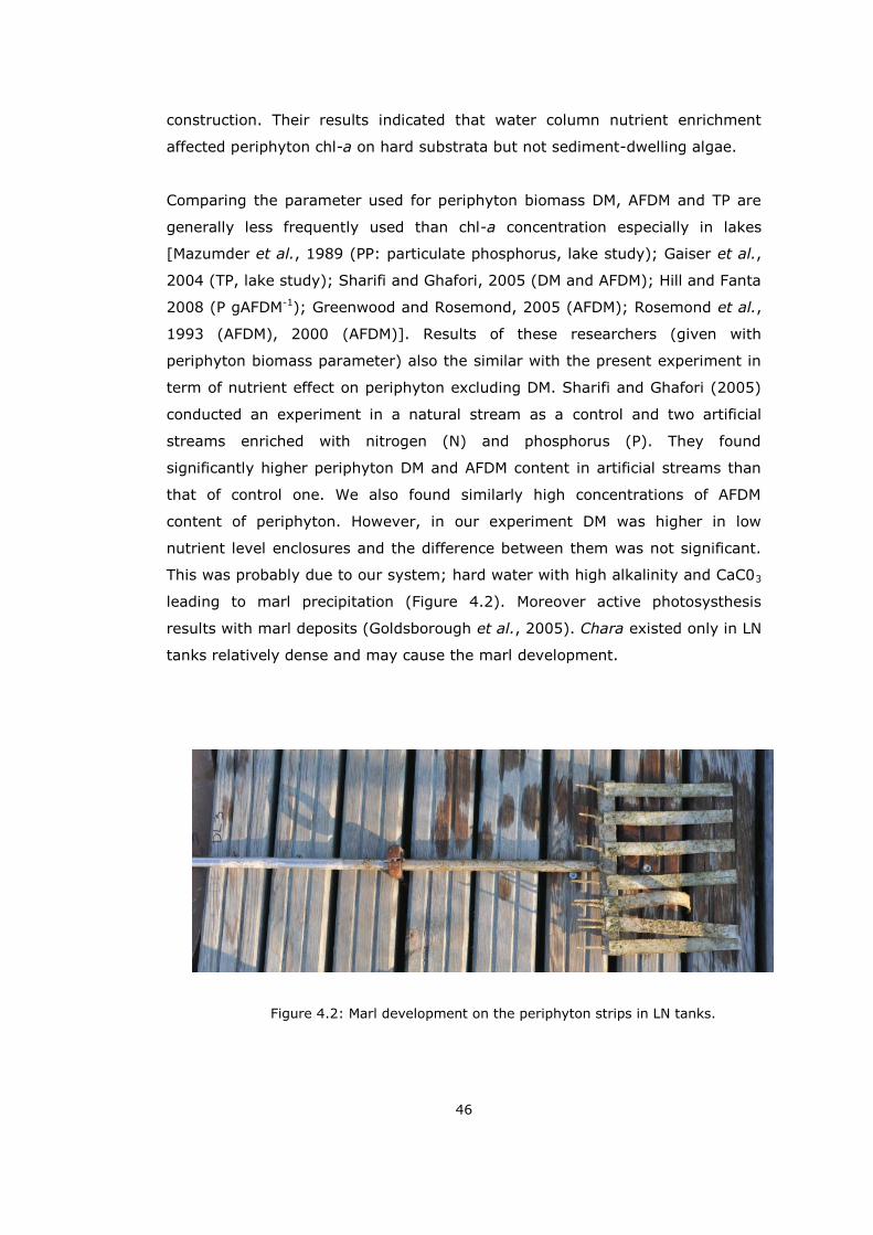
46

construction. Their results indicated that water column nutrient enrichment

affected periphyton chl-a on hard substrata but not sediment-dwelling algae.

Comparing the parameter used for periphyton biomass DM, AFDM and TP are

generally less frequently used than chl-a concentration especially in lakes

[Mazumder et al., 1989 (PP: particulate phosphorus, lake study); Gaiser et al.,

2004 (TP, lake study); Sharifi and Ghafori, 2005 (DM and AFDM); Hill and Fanta

2008 (P gAFDM-1); Greenwood and Rosemond, 2005 (AFDM); Rosemond et al.,

1993 (AFDM), 2000 (AFDM)]. Results of these researchers (given with

periphyton biomass parameter) also the similar with the present experiment in

term of nutrient effect on periphyton excluding DM. Sharifi and Ghafori (2005)

conducted an experiment in a natural stream as a control and two artificial

streams enriched with nitrogen (N) and phosphorus (P). They found

significantly higher periphyton DM and AFDM content in artificial streams than

that of control one. We also found similarly high concentrations of AFDM

content of periphyton. However, in our experiment DM was higher in low

nutrient level enclosures and the difference between them was not significant.

This was probably due to our system; hard water with high alkalinity and CaC03

leading to marl precipitation (Figure 4.2). Moreover active photosysthesis

results with marl deposits (Goldsborough et al., 2005). Chara existed only in LN

tanks relatively dense and may cause the marl development.

Figure 4.2: Marl development on the periphyton strips in LN tanks.

47

Hill and Fanta (2008) showed that soluble reactive phosphorus (SRP) and

periphyton phosphorus content was related in a nonlinear way. Here

phosphorus of periphyton reached a maximum at 82 µg l-1 SRP. Thereby

between the SRP range of our experiment (LN: 2.07, HN: 13.01 µg l-1) and

further TP of periphyton rose with increasing nutrient concentrations.

DM, AFDM, TP and chl-a of periphyton decreased with time in both HN and LN

enclosures. But, at the last sampling all periphyton parameters increased in LN

tanks and Bonferroni test showed that TP and chl-a amount of periphyton

statistically increased. Was it random or significant? Actually TP concentrations

of water column in enclosures (Figure 3.8) also increased and Bonferroni test

showed the raise of the last month was significant and it was coincided with the

raise of periphyton biomass of LN tanks. Thus, significant phosphorus increase

of enclosures might have affected the LN periphyton biomass. But then the

same effect was not observed in the HN tanks. It is probably because nutrient

addition to shallow lakes which had low nutrient level were more affected than

the lakes had high nutrient level and also in low nutrient levels, uptake of

nutrients and response to them is faster (Noe et. al.,2003; Hwang et al., 1998).

Moreover decreasing of grazing pressure might cause the raise of periphyton

biomass in LN tanks. Because of the decreasing temperature, chironomidae

larvae could decrease and reduce the grazing pressure on the periphyton

biomass (Liboriussen et al., 2003).

On the other hand grazer experiment showed that grazing pressure in HN tanks

increased through time. Since periphyton biomass in HN tanks decreased under

high nutrient and high grazing conditions, this observation might lead to an

understanding that grazing effect has more impact on periphyton growth than

nutrients have. While Phillips et al., (1978) revealed that nutrient effect is

stronger than gazer pressure on periphyton; Jones and Sayer (2003) found a

significant relationship between grazers and periphyton but not between

phosphorus concentration and periphyton.

48

4.3 Macrophytes and Periphyton

Studies (e. g. James et al., 2005; Baker, 2010) showed that macrophyte

abundance decreases with the increasing nutrients. However in our experiment

although the difference between LN and HN tanks was not important

significantly, the plant we used Myriophyllum spicatum was much more in HN

tanks. On the other hand while HN enclosures had only M. spicatum LN tanks

had not only it but also Chara contraria that is known as an indicator of low

nutrient conditions with a significant difference. Two main reasons can be

accounted for both nutrient level enclosures had likely the same abundance of

M. spicatum. Firstly; it was less in LN tanks because existence C. contraria

could cause a competition with M. spicatum for nutrient supply and limit its

growth, M. spicatum is a plant which also compete with other macrophytes for

nutrients (Smith et al.,2002). Blindow et al. (2002) observed that dense Chara

(app. half of the lake) caused a decrease in chlorophyll and phosphorus

concentrations. Secondly; it did not decrease with high nutrient levels in HN

tanks because the dropping water level increases light availability for

macrophytes and often coincides with a raise in residence time (Beklioğlu et al.,

2006, 2008; Bucak, 2012). Smith et al. (2002) revealed that while in low

nitrogen conditions autofragments and stems of M. spicatum developed more,

in high nutrient conditions stems and root parts developed greater. This may

lead to longer residence time in high nutrient levels.

In HN tanks despite the high nutrient, Myriophyllum spicatum grew in the

beginning of the experiment because planktonic chl-a was low and so water

was clear enough to allow early growth of the plant. However, the later growth

appeared to be controlled by the periphytopn growth as the macrophyte PVI%

and periphytic chl-a concentration showed the opposite trend such as in July

and August but more clearly and strongly in September. Despite the high level

of planktonic chl-a in the water column, macrophyte kept growing since M.

spicatum already grew until August, high level of planktonic chl-a itself did not

set a light limitation for the macrophyte (Figure 4.3).

49

In LN tanks, PVI% of M. spicatum increased to approx. 15% in September but

then it started to decrease probably as a response to increased periphyton

biomass. Furthermore, competition with Chara might have reinforced the

reduction. On the other hand, in LN tanks Chara grew well because of the low

nutrient and consequently clear water conditions during the experiment.

Though it was not easy to estimate Chara coverage and PVI% beacuse of the

depth induced visibility problem as well as the short stature of the plant

unabling measurement. Harvesting the plant at the end of the experiment

explicity showed that we had strong Chara growth (Figure 3.19, Table 3.3)).

Thus it appeared to be that for chara growth, periphyton did not have a major

effect prorbably because of allelopathy effect of Chara on periphyton via

excreting cupper sulphate (Figure 4.3).

The results of epiphyton which was taken at the end of our experiment from M.

Spicatum also supperted the periphyton biomass results of artificial substrates.

It showed that DM, AFDM and TP were not different significantly despite they

were much more in HN tanks. On the other hand chlorophyll-a concentrations

are significantly different. It is because periphyton experiment ended in October

however macrophytes were harvested in November at the end of the mesocosm

experiment. Thus dead cells increased on macrophytes and as it was shown in

Table 1.1, these parameters also include dead cells. On the other hand, since

chl-a is spesific to algae, there was a significant difference between HN and LN

tanks (Figure 3.21).

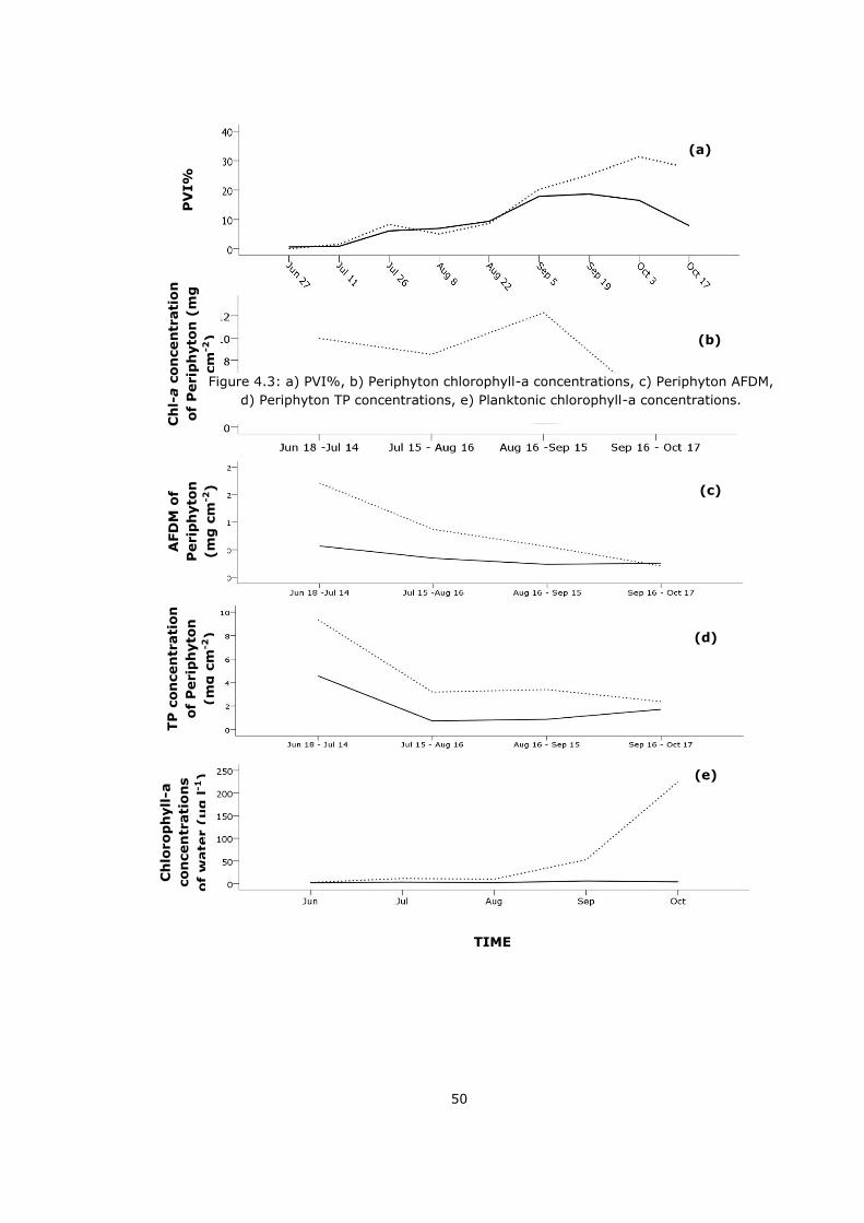
50

PV

I%

C

hl-

a c

on

cen

trati

on

of

Perip

hyto

n (

mg

cm

-2)

AFD

M o

f

Perip

hyto

n

(m

g c

m-2

)

TP

con

cen

trati

on

of

Perip

hyto

n

(m

g c

m-2

)

Ch

lorop

hyll

-a

con

cen

trati

on

s

of

wate

r (µ

g l

-1)

TIME

Figure 4.3: a) PVI%, b) Periphyton chlorophyll-a concentrations, c) Periphyton AFDM,

d) Periphyton TP concentrations, e) Planktonic chlorophyll-a concentrations.

(a)

(b)

(c)

(d)

(e)

51

4.4 Macroinvertebrates and Periphyton

Although difference of macroinvertebrate abundance was not significant

between HN and LN tanks, low nutrient level enclosures have more diverse and

more macroinvertebrates because of the fish grazer pressure (Mazumder et al.,

1989) and nutrient level differences (Liboriussen et al., 2005).

In our tanks we observed just three groups of macroinvertebrates which were

gastropod, oligacheta and chiromidae (Table 3.1). Periphyton is an important

resource for chironomids as a habitat and also as food (Liboriussen et al.,

2005). Also gastropods are one of the important grazers feeding on periphyton

(Hillebrand and Kahlert, 2001). Researchs show that oligochaeta concentrations

are increasing with increasing periphyton (Kilroy et al., 2009; Friberg et al.,

2003). In LN tanks these three groups were more abundant and it was resulted

with a lower concentrations of periphyton biomass.

There was not so many diverse macroinvertebrates in sediment samples.

Therefore Chironomidae family was identified to species level to compare the

nutrient levels better. However the species could not be compared with the

statistical programme because of insufficient data. We should have taken more

than 3 kajak cores. But considering the abundance of species, we may say that

Chironomus dorsalis, Cryptochironomus defectus and Kiefferulus

tendipediformis can not modify the high nutrient conditions. Besides

Chironomus nuditarsis may be an indicator for the increasing nutrient

conditions.

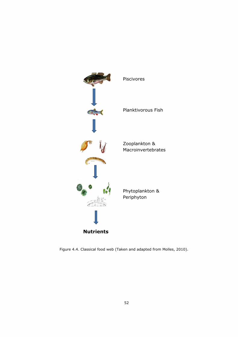
52

Figure 4.4. Classical food web (Taken and adapted from Molles, 2010).

Piscivores

Planktivorous Fish

Zooplankton &

Macroinvertebrates

Nutrients

Phytoplankton &

Periphyton

53

4.5 Top-down, Bottom-up Effect

All periphytic algae are not affected from grazers in the same way, all grazing

invertebrates are not a good prey for fish as well. Moreover invertebrates and

also periphytic algae can exhibit behavioral responses to predation. After all the

cascade between predators, herbivores and producers seem to be strong

(Figure 4.4), (Jones and Sayer, 2003).

In the beginning of our experiment all conditions were the same except nutrient

level (Figure 4.4). At the end of the experiment we saw more fish, less

macroinvertebrate and more periphyton abundance in LN tanks, while less fish,

more macroinvertebrates and less periphyton in HN tanks (Figure 4.5, 4.6,

3.13, 3.14, 3.15). Considering bottom-up effect high nutrient much more

increased primary production in HN enclosures via rising phytoplankton and

periphyton abundance than LN tanks. This raise increased macroinvertebrates

which feed on periphyton and increased fish which feed on macroinvertebrates.

In our enclosures there was planktivorous fish but not piscivorous fish. Hence

amount of planktivorus fish much more increased in HN enclosures than LN

ones (Table 3.3, 3.4). This had a strong cascading effect of fish on periphyton

via grazers that included macroinvertebrates and zooplankton. Thus we had

limited the grazer effect on periphyton and periphyton composition much more

increased in high nutrient level enclosures. Despite same number of fish

inoculum to every enclosure, HN tanks developed more fish. Hence, despite the

same top-down control effect at the start of the experiment, top down control

of fish via periphyton grazers also varied with nutrients reflecting the bottom-

up effect (Mazumder et al., 1989; Jones and Sayer, 2003).

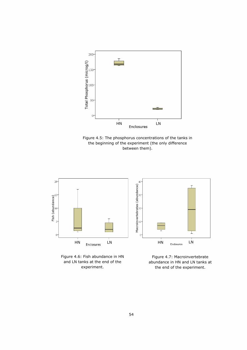
54

Figure 4.5: The phosphorus concentrations of the tanks in

the beginning of the experiment (the only difference

between them).

Figure 4.6: Fish abundance in HN

and LN tanks at the end of the

experiment.

Figure 4.7: Macroinvertebrate

abundance in HN and LN tanks at

the end of the experiment.

HN LN

HN HN LN LN

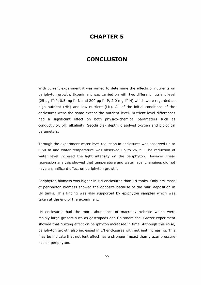
55

CHAPTER 5

CONCLUSION

With current experiment it was aimed to determine the effects of nutrients on

periphyton growth. Experiment was carried on with two different nutrient level

(25 µg l-1 P, 0.5 mg l-1 N and 200 µg l-1 P, 2.0 mg l-1 N) which were regarded as

high nutrient (HN) and low nutrient (LN). All of the initial conditions of the

enclosures were the same except the nutrient level. Nutrient level differences

had a significant effect on both physico-chemical parameters such as

conductivity, pH, alkalinity, Secchi disk depth, dissolved oxygen and biological

parameters.

Through the experiment water level reduction in enclosures was observed up to

0.50 m and water temperature was observed up to 26 ºC. The reduction of

water level incresed the light intensity on the periphyton. However linear

regression analysis showed that temperature and water level changings did not

have a sihnificant effect on periphyton growth.

Periphyton biomass was higher in HN enclosures than LN tanks. Only dry mass

of periphyton biomass showed the opposite because of the marl deposition in

LN tanks. This finding was also supported by epiphyton samples which was

taken at the end of the experiment.

LN enclosures had the more abundance of macroinvertebrate which were

mainly large grazers such as gastropods and Chironomidae. Grazer experiment

showed that grazing effect on periphyton increased in time. Although this raise,

periphyton growth also increased in LN enclosures with nutrient increasing. This

may be indicate that nutrient effect has a stronger impact than grazer pressure

has on periphyton.

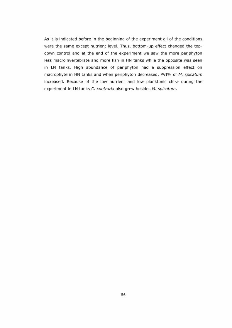
56

As it is indicated before in the beginning of the experiment all of the conditions

were the same except nutrient level. Thus, bottom-up effect changed the top-

down control and at the end of the experiment we saw the more periphyton

less macroinvertebrate and more fish in HN tanks while the opposite was seen

in LN tanks. High abundance of periphyton had a suppression effect on

macrophyte in HN tanks and when periphyton decreased, PVI% of M. spicatum

increased. Because of the low nutrient and low planktonic chl-a during the

experiment in LN tanks C. contraria also grew besides M. spicatum.

57

REFERENCES

Azim M. E. (2001), The potential of periphyton-based aquaculture production

systems. Doctoral Dissertation, Fish Culture and Fisheries Group, Wageningen

Institute of Animal Sciences (WIAS), Wageningen University, The Netherlands.

Azim M. E., Wahab M. A., Biswas P. K., Asaeda T., Fujino T. and Verdegem M.

C. J. (2004), The effecmt of periphyton substrate density on production in

freshwater polyculture ponds. Aquaculture, 232: 441-453.

Azim M. E. and Asaeda T. (2005), Periphyton structure, diversity and

colonization. In: Azim M. E., Verdegem M. C. J., van Dam A. A. And Beveridge

M. C. M. (eds), Periphyton: Ecology, Exploitation and Management, CABI Publ.,

UK, pp. 15-33.

Azim M. E., Beveridge M. C. M., van Dam A. A. and Verdegem M. C. J. (2005),

Periphyton and Aquatic Production: an Introduction. In: Azim M. E., Verdegem

M. C. J., van Dam A. A. And Beveridge M. C. M. (eds), Periphyton: Ecology,

Exploitation and Management, CABI Publ., UK, pp. 1-13.

Bachmann R. W., Horsburgh C. A., Hoyer M. V., Matazara L. K. and Canfield Jr.

D. E. (2002), Relations between trophic state indicators and plant biomass in

Florida lakes. Hydrobiologie, 470: 219-234.

Bailey R. C., Norris R. and Reynoldson T. (2004), Bioassessment of Freshwater

Ecosystems: Using the Reference Condition Approach. Kluwer Academic

Publishers, New York.

Bakker E. S., Donka E. V., Declercka S. A. J., Helmsinga N. R., Hiddinga B. and

Nolet B. A. (2010), Effect of macrophyte community composition and nutrient

58

enrichment on plant biomass and algal blooms. Basic and Applied Ecology, 11:

432–439.

Bécares E., Gomá J., Fernández-Aláez M., Fernández-Aláez C., Romo S., Miracle

M. R., Ståhl-Delbanco A., Hansson L., Gyllström M., Ven de Bund W. J., Donk E.

V., Kairesalo T., Hietala J., Stephen D., Balayla D. and Moss B. (2008), Effects

of nutrients and fish on periphyton and plant biomass across a European

latitudinal gradient. Aquatic Ecology, 42: 561-574.

Beklioglu M. and Tan C. O. (2008), Restoration of a shallow Mediterranean lake

by biomanipulation complicated by drought. Fundamental and Applied

Limnology, 171: 105–118.

Beklioglu M., Altinayar G. and Tan C. O. (2006), Water level control over

submerged macrophyte development in five shallow lakes of Mediterranean

Turkey. Archiv für Hydrobiologie, 166: 535–556.

Beresford A. L. and Jones J. I. (2010), Weedbeds and big bugs: the importance

of scale in detecting the influence of nutrients and predation on

macroinvertebrates in plant-dominated shallow lakes. Freshwater Biology, 55:

514–530.

Blindow I., Hargeby A. and Anderson G. (2002), Seasonal changes of

mechanisms maintaining clear water in a shallow lake with abundant Chara

vegetation. Aquatic Botany, 72: 315–334.

Boston H. L. and Hill W. R. (1991), Photosynthesis-light relations of stream

periphyton communities. Limnology and Oceanography, 36(4): 644-656.

Bothwell M. L. (1988), Growth-rate responses of lotic periphytic diatoms to

experimental phosphorus enrichment - the influence of temperature and light.

Canadian Journal of Fisheries and Aquatic Sciences, 45: 261-270.

Bowes M. J., Lehmann K., Jarvie H. And Singer A. C. (2010), Investigating

periphyton response to changing phosphorus concentrations in UK rivers using

59

within-river flumes. British Hydrological Society Managing Consequences of a

Changing Global Environment, Newcastle.

Bucak T., Saraoglu E., Levi E. E., Tavsanoglu Ü. N., Çakıroğlu A. İ., Jeppesen E.

and Beklioğlu M. (2012), The influence of water level on macrophyte growth

and trophic interactions in eutrophic Mediterranean shallow lakes: a mesocosm

experiment with and without fish. Freshwater Biology, 57: 1631–1642.

Burkholder J. M. and Wetzel R. G. (1990), Epiphytic alkaline phosphatase on

natural and artificial plants. Limnology and Oceanogrophy, 35(3): 736-747.

Cattaneo A. and Mousseau B. (1995), Empirical analysis of the removal rate of

periphyton by grazers. Oecologia, 103: 249–254.

Chételat J., Pick F. R., Morin A. and Hamilton P. B. (1999), Periphyton biomass

and community composition in rivers of different nutrient status. Canadian

Journal of Fisheries and Aquatic Sciences, 56: 560–569.

Costanza R., d’Arge R., de Groot R., Farber S., Grasso M., Hannon B., Limburg

K., Naeem S., O’neill R. V., Paruelo J., Raskin R. G., Sutton P. and van den Belt

M. (1997), The value of the world’s ecosystem services and natural capital.

Nature, 387: 253–260.

DeNicola D. M. (1996), Periphyton responses to temperature at different

ecological levels. In: Stevenson R. J., Bothwell M. L. And Lowe R. L. (Eds.),

Algal Ecology – Freshwater Benthic Ecosystems. Academic Press, San Diego,

California pp. 149–81.

Downing J. A., Plante C. and Lalonde S. (1990), Fish production correlated with

primart prioductivity and morpoedaphic index. Canadian Journal of Fisheries

and Aquatic Sciences, 47: 1929–1936.

Dudgeon D., Arthington A. H., Gessner M. O., Kawabata Z., Knowler D. J.,

Lévéque C., Naiman R. J., Prieur-Richard A. H., Soto D., Stiassny M. L. and

Sullivan C. A. (2006), Freshwater biodiversity: importance threats status and

conservation challenges. Biological Reviews, 81(02): 163–182.

60

Eminson D. and Moss B. (2007), The composition and ecology of periphyton

communities in freshwaters. British Phycological Journal, 15 (4): 429-446.

Friberg N., Lindstrøm M., Kronvang B. and Larsen S. E. (2003),

Macroinvertebrate/sediment relationships along a pesticide gradient in Danish

streams. Hydrobiologia, 494: 103–110, 2003.

Gaiser E. E., Scintoa L. J., Richards J. H., Jayachandran K., Childers D. L.,

Trexler J. C. and Jones R. D. (2004), Phosphorus in periphyton mats provides

the best metric for detecting low-level P enrichment in an oligotrophic wetland.

Water Research, 38: 507–516.

Gasith A. and Hoyer M.V. (1998), Structuring role of macrophytes in lakes:

changing influence along lake size and depth gradients. In Jeppesen E.,

Søndergaard Ma., Søndergaard Mo. and Christoffersen K. (eds), The Structuring

Role of Submerged Macrophytes in Lakes, pp. 381–392. Springer-Verlag New

York USA.

Goldsborough L. G. and Robinson G. G. C. (1996), Pattern in wetlands. In:

Stevenson R. J., Bothwell M. L. and Lowe R. L. (eds), Algal ecology: Freshwater

benthic ecosystems. Academic Press, New York, pp. 77-117.

Goldsborough L. G., McDougal R. L. and North A. K. (2005), Periphyton in

freshwater lakes and wetlands. In: Azim M. E., Verdegem M. C. J., van Dam A.

A. And Beveridge M. C. M. (eds), Periphyton: Ecology, Exploitation and

Management, CABI Publ., UK, pp. 71-89.

Greenwood J. L. And Rosemond A. D. (2005), Periphyton response to long-term

nutrient enrichment in a shaded headwater stream. Canadian Journal of

Fisheries and Aquatic Sciences, 62: 2033-2045.

Gross E. M, Feldbaum C. and Graf A. (2003), Epiphyte biomass and elemental

composition on submersed macrophytes in shallow eutrophic lakes.

Hydrobiologia, 506(509): 559-565.

61

Hansson L. A. (1992), Factors regulating periphyton biomass. Limnology and

Oceanogrophy, 37: 322-328.

Hecky R. E. and Hesslein R. H. (1995), Contributions of benthic algae to lake

food webs as revealed by stable isotope analysis. Journal of North Amer

Benthological Society, 14(4): 631-653.

Hill W. R. And Fanta S. E. (2008), Phosphorus and light colimit periphyton

growth at subsaturating irradiances. Freshwater Biology, 53: 215-225.

Hillebrand H. And Kahlert M. (2002), Effect of grazing and water column

nutrient supply on biomass and nutrient content of sediment microalgae.

Aquatic Botany, 72: 143-159.

Hoagland K. D., Roemer S. C. and Rosowski J. R. (1982), Colonization and

community structure of two periphyton assemblages with emphasis on the

diatoms (Bacillariophyceae), American Journal of Botany, 69: 188-213.

Hudon C. and Bourget E. (1981), Initial colonization of artificial substrate:

community development and structure studied by scanning electron

microscopy. Canadian Journal of Fisheries and Aquatic Sciences, 38: 449-457.

Hwang S., Havens K. E. and Steinman A. D. (1998), The use of aquatic

macrophytes in water-pollution control. Freshwater Biology, 40: 729-745.

James C., Fisher J., Russell V., Collings S. and Moss B. (2005), Nitrate

availability and hydrophyte species richness in shallow lakes. Freshwater

Biology, 50: 1049–1063.

Jeppesen E., Søndergaard Ma., Søndergaard Mo. and Christoffersen K. (1998),

The Structuring Role of Submerged Macrophytes in Lakes. Springer-Verlag, New

York Inc.

Jones J. I. and Sayer C. D. (2003), Does the fish-invertebrate-periphyton

cascade precipitate plant loss in shallow lakes? Ecology, 84(8): 2155-2167.

62

Kahlert M and Pettersson K. (2002), The impact of substrate and lake trophy on

the biomass and nutrient status of benthic algae. Hydrobiologia, 489: 161-169.

Kilroy C., Larned S. T. and Biggs B. J. F. (2009), The non-indigenous diatom

Didymosphenia geminata alters benthic communities in New Zealand rivers.

Freshwater Biology, 54: 1990–2002.

Köhler J., Hachoł J. and Hilt S. (2010), Regulation of submersed macrophyte

biomass in a temperate lowland river: Interactions between shading by bank

vegetation, epiphyton and water turbidity. Aquatic Botany 92: 129-136.

Liboriussen L. and Jeppesen E. (2003), Temporal dynamics in epipelic, pelagic

and epiphytic algal production in a clear and a turbid shallow lake. Freshwater

Biology, 48: 418-431.

Liboriussen L., Jeppesen E., Bramm M. E. and Lassen M. F. (2005), Periphyton-

macroinvertebrate interactions in light and fish manipulated enclosures in a

clear and a turbid shallow lake. Aquatic Ecology, 39: 23-39.

Liboriussen L. and Jeppesen E. (2006), Structure, biomass, production and

depth distribution of periphyton on artificial substratum in shallow lakes with

contrasting nutrient concentrations. Freshwater Biology, 52: 95-109.

Loeb S. L., Reuter J. E. and Goldman C. R. (1983), Littoral zone production of

oligotrophic lakes – the contributions of phytoplankton and periphyton. In:

Wetzel R. G. (eds), Periphyton of Freshwater Ecosystems. Developments in

Hydrobiology, Volume 17, Dr. Junk Publishers, The Hague, The Netherlands, pp.

161-167.

Loeb S. L. and Reuter J. E. (1981), The epilithic community: a five lake

comparative study of community productivity nitrogen metabolism and depth

distribution of standing crop. Verhandlungen internationale Vereinigung fur

theoretische und angewandte Limnologie, 21: 346-352.

63

Lowe R. L. (1996), Periphyton patterns in lakes. In: Stevenson R. J., Bothwell

M. L. and Lowe R. L. (eds), Algal ecology: Freshwater benthic ecosystems.

Academic Press, New York, pp. 57-76.

Marcus M. D. (1980), Perıphytic community response to chronic nutrient

enrichment by a reservoir discharge. Ecology, 61(2): 387-399.

Maltais M. J. And Vincent W. F. (1997), Periphyton community structure and

dynamics in a subarctic lake. Canadian Journal of Botany, 75: 1556-1569.

Mazumder A., Taylor W. D., McQueen J. and Lean D. R. S. (1989), Effects of

nutrient and grazers on periphyton phosphorus in lake enclosures. Freshwater

Biology, 22: 405-415.

Meerhoff M., Beklioglu M., Burks R., García-Rodríguez F., Mazzeo N. and Moss

B. (2010), Shallow lakes: preface. Hydrobiologia, 646: 1–3.

Meulemans J. T. and Roos P. J. (1985), Structure and architecture of the

periphyton community on dead reed stems in Lake Maarsseveen. Archiv für

Hydrobiologie, 102: 487–502.

Milstein A. (2005), Effect of periphyton on water quality. In: Azim M. E.,

Verdegem M. C. J., van Dam A. A. And Beveridge M. C. M. (eds), Periphyton:

Ecology, Exploitation and Management, CABI Publ., UK, pp. 179-190.

Moss B. (2010), Ecology of freshwaters: A view for the twenty-first century.

WileyScience, 4th edition.

Naiman R., Magnuson J., McKnight D. and Stanford J. (1995), The Freshwater

Imperative: A Research Agenda, Island Press Washington D.C.

Neundorfer J. V. and Kemp W. M. (1993), Nitrogen versus phosphorus

enrichment of brackish waters: responses of the submersed plant Potamogeton

perfoliatus and its associated algal community. Marine Ecology Progress Series,

94: 71-82.

64

Noe G. B., Scinto L. J., Taylor J., Childers D. L. and Ronal D. J. (2003),

Phosphorus cycling and partitioning in an oligotrophic Everglades wetland

ecosystem: a radioisotope tracing study. Freshwater Biology, 48: 1993-2008.

NOFDIANTO Research Center for Limnology Indonesian Institute of Sciences

(2011), Growth response of algal periphyton to light and temperature.

Oseanologi dan Limnologi di Indonesia, 37(1): 155–169.

Özkan K., Jeppesen E., Johansson L. S. And Beklioğlu M. (2010), The response

of periphyton and submerged macrophytes to nitrogen and phosphorus loading

in shallow warm lakes: a mesocosm experiment. Freshwater Biology, 55: 463-

475.

Peterson B. J. and Howarth R. (1987), Sulfur, carbon and nitrogen isotopes

used to trace organic matter flow in the salt-marsh estuaries of Sapelo Island,

Georgia. Limnology and Oceanography, 32: 1195-1213.

Phillips G. L., Eminson D. and Moss B. (1978), Mechanisms to account for

macrophyte decline in progressively eutrophicated freshwaters. Aquatic Botany,

4: 103–126.

Reid G. K. and Wood R. D. (1976), Ecology of Inland Waters and Estuarie, 2nd

edition, D. van Nostrand Company, New York.

Roberts E., Kroker J., Körner S. and Nicklisch A. (2003), The role of periphyton

during the re-colonization of a shallow lake with submerged macrophytes.

Hydrobiologia, 506(509): 525-530.

Rosemond A. D., Mulholland P. J. and Brawley S. H. (2000), Seasonally shifting

limitation of stream periphyton: response of algal populations and assemblage

biomass and productivity to variation in light, nutrients, and herbivores.

Canadian Journal of Fisheries and Aquatic Sciences, 57: 66-75.

Rosemond A. D., Mulholland P. J. and Elwood J. W. (1993), Top-down and

bottom-up control of stream periphyton: effects of nutrients and herbivores.

Ecology, 74: 1264–1280.

65

Sabater S. And Admiraal W. (2005), Periphyton as biological indicators in

managed aquatic ecosystems. In: Azim M. E., Verdegem M. C. J., van Dam A.

A. And Beveridge M. C. M. (eds), Periphyton: Ecology, Exploitation and

Management, CABI Publ., UK, pp. 159-177.

Scheffer M. (1998), Ecology of Shallow Lakes. Chapman and Hall, London.

Scheffer M., Carpenter S., Foley J. A., Folke C. and Walkerk B. (2001),

Catastrophic shifts in ecosystems. Nature, 413: 591–596.

Scheffer M., Hosper S., Meijer M. L., Moss B. and Jeppesen E. (1993),

Alternative equilibria in shallow lakes. TREE, 8: 257–278.

Sánchez M. L., Pizarro H. Tell G. and Izaguirre I (2010), Relative importance of

periphyton and phytoplankton in turbid and clear vegetated shallow lakes from

the Pampa Plain (Argentina): a comparative experimental study. Hydrobiologia,

646: 271–280.

Sharifi M. And Ghafori M. (2005), Effects of added nutrients on dry mass, ash

free dry mass, chlorophyll-a and biovolume of periphyton algae in aritificial

streams. Iranian Journal of Science and Technology, 29: 29-38.

Smith S. M. and Lee K. D. (2006) Responses of periphyton to artificial nutrient

enrichment in freshwater kettle ponds of Cape Cod National Seashore.

Hydrobiologia, 571: 201–211.

Smith D. H., Madsen J. D., Dickson K. L.and Beitinger T. L. (2002), Nutrient

effects on autofragmentation of Myriophyllum spicatum. Aquatic Botany, 74: 1–

17.

Vadeboncoeur Y., Zanden M. J. V. And Lodge D. M. (2002), Putting the Lake

Back Together: Reintegrating Benthic Pathways into Lake Food Web Models.

BioScience, 52(1): 44-54.

66

Van Dam A. A., Beveridge M. C. M., Azim M. E. and Verdegem M. C. J. (2002),

The potential of fish production based on periphyton, Reviews in Fish Biology

and Fisheries, 12: 1-31.

Van Dam A. A. and Verdegem M. C. J. (2005), Utilization of periphyton for fish

production in ponds: a system ecology perspective. In: Azim M. E., Verdegem

M. C. J., van Dam A. A. And Beveridge M. C. M. (eds), Periphyton: Ecology,

Exploitation and Management, CABI Publ., UK, pp. 91-111.

Van Dam H. M, Mertens A. and Sinkeldam J. (1994), A coded checklist and

ecological indicator values of freshwater diatoms from The Netherlands.

Netherland Journal of Aquatic Ecology, 28: 117-133.

Vermaat J. E. (2005), Periphyton dynamics and influencing Factors. In: Azim M.

E., Verdegem M. C. J., van Dam A. A. And Beveridge M. C. M. (eds),

Periphyton: Ecology, Exploitation and Management, CABI Publ., UK, pp. 35-49.

Vermaat J. E. and Hootsmans M. J. M. (1994), Periphyton dynamics in a

temperature-light gradient. In: van Vierssen W., Hootsmans M. J. M. and

Vermaat J. E. (eds) Lake Veluwe a Macrophytedominated System under

Eutrophication Stress. Kluwer Academic Publishers Dordrecht, The Netherlands

pp. 193–212.

Welcomme R. L. (2005), Traditional Brush Park Fisheries in natural waters. In:

Azim M. E., Verdegem M. C. J., van Dam A. A. And Beveridge M. C. M. (eds),

Periphyton: Ecology, Exploitation and Management, CABI Publ., UK, pp. 141-

157.

Wetzel R. G. (2001), Limnology: Lake and River Ecosystems. Academic Press,

San Diego, California, USA, 3rd edition.

Wetzel R. G. (2005), Periphyton in the aquatic ecosystem amd food webs. In:

Azim M. E., Verdegem M. C. J., van Dam A. A. And Beveridge M. C. M. (eds),

Periphyton: Ecology, Exploitation and Management, CABI Publ., UK, pp. 51-69.

67

Williamson C. E., Saros J. E. and Schindler D. W. (2009), Sentinels of change.

Science, 323(5916): 887–888.

impacts of nutrients on periphyton growth and periphyton-macroinvertebrates...

Documents