impacts of re-colonizing gray wolves on mule deer and
TRANSCRIPT
Impacts of Re-colonizing Gray Wolves
on Mule Deer and White-tailed Deer in North-Central Washington
Justin Aaron Dellinger
A dissertation
submitted in partial fulfillment of the
requirements for the degree of
Doctor of Philosophy
University of Washington
2018
Reading Committee:
Aaron Wirsing, Chair
James Anderson
Kurt Jenkins
Brian Kertson
Program Authorized to Offer Degree:
School of Environmental and Forest Sciences

©Copyright 2018
Justin Aaron Dellinger
University of Washington
Abstract
Impacts of Re-colonizing Gray Wolves
on Mule Deer and White-tailed Deer in North-Central Washington
Justin Aaron Dellinger
Chair of the Supervisory Committee:
Assistant Professor Aaron J. Wirsing
School of Environmental and Forest Sciences
Previous research on gray wolves (Canis lupus) in protected landscapes demonstrates these large
carnivores can have consumptive and non-consumptive effects on prey species which lead to
top-down trophic cascades. However, much remains to be known about impacts of gray wolves
on prey in managed landscapes as well as how these predators influence interactions between
prey species. Recent natural re-colonization of gray wolves to managed landscapes of
Washington state facilitated a natural experiment wherein we explored impacts of gray wolves
on multiple sympatric prey species – mule deer (Odocoileus hemionus) and white-tailed deer (O.
virginianus). We compared survival, habitat use, and resource partitioning of adult mule deer and
adult white-tailed deer in wolf present and wolf absent areas. Mule deer and white-tailed deer
survival rates were not negatively impacted by presence of gray wolves. Season was the primary
factor in explaining all predator and human-caused mortality. Our data suggests gray wolves may
not have consumptive effects on native prey populations in Washington state. Next, mule deer

and white-tailed deer experiencing gray wolf predation risk did exhibit shifts in habitat use
relative to conspecifics in areas without gray wolves. Shifts in habitat use by mule deer and
white-tailed occurred at coarse and fine-spatial scales, respectively, and were explained by
divergent escape tactics of each prey species and the landscape features that promote escape of
each deer species when facing gray wolf predation risk. It appears gray wolves can influence
habitat use of multiple prey species and potentially at differing spatial scales depending on
escape behavior of prey species and the landscape features that promote escape of prey from
predation. Our results suggest gray wolves could initiate multiple top-down trophic cascades via
prey species specific shifts in habitat use in response to gray wolf predation risk. Lastly, there
was increased resource partitioning between mule deer and white-tailed deer in areas with gray
wolves compared to resource partitioning between mule deer and white-tailed deer in areas
without gray wolves. Increased resource partitioning between mule deer and white-tailed deer
was again explained by divergent escape tactics of each prey species and the landscape features
promoting escape of each deer species subject to wolf predation risk. However, direction and
magnitude of resource partitioning between mule deer and white-tailed in areas with gray wolves
compared to areas without gray wolves varied with season and scale. Our findings demonstrate
that gray wolf predation risk can mediate interactions between co-occurring prey species but is
context-dependent. We suggest further research on consumptive and non-consumptive effects of
gray wolves on multiple prey species to better understand the potential for top-down trophic
cascades in managed landscapes.
i
Table of Contents
List of Figures……………………………………………………………………………………..ii
List of Tables…………………………………………………………………………….………..iv
General Introduction…………….………………………………………………………………...1
Literature Cited……………………………………………………………………………………6
Chapter 1: Impacts of recolonizing gray wolves on survival and mortality in two sympatric
ungulates…………………………………………………………………………………………..9
Abstract……………………………………………………………………………………9
Introduction………………………………………………………………………………10
Materials and Methods…………………………………………………………………...13
Study Area……………………………………………………………….……….13
Data Collection…………………………………………………………………...15
Analyses………………………………………………………………………….18
Results……………………………………………………………………………………20
Discussion………………………………………………………………………………..21
Literature Cited…………………………………………………………………………..28
Chapter 2: Escape behavior predicts divergent anti-predator responses of sympatric prey to
recolonizing gray wolves…………………………………………………………………………40
Abstract…………………………………………………………………………………..40
Introduction………………………………………………………………………………41
Materials and Methods…………………………………………………………………...44
Study Area………………………………………………………………………..44
Data Collection…………………………………………………………………...46
Analyses………………………………………………………………………….47
Results……………………………………………………………………………………50
Discussion………………………………………………………………………………..52
Literature Cited…………………………………………………………………………..60
Supplementary Material………………………………………………………………….65
Chapter 3: Do recolonizing gray wolves impact resource partitioning among sympatric prey
species? ………………………………………………………………………………………….79
Abstract…………………………………………………………………………………..79
Introduction………………………………………………………………………………80
Materials and Methods…………………………………………………………………...84
Study Area………………………………………………………………………..84
Data Collection…………………………………………………………………...84
Analyses………………………………………………………………………….85
Results……………………………………………………………………………………91
Discussion………………………………………………………………………………..94
Literature Cited…………………………………………………………………………104
ii
List of Figures
Figure 1.1. Location of the study area (11N 372208 E, 5389786 N) in Washington, USA, which
included two areas occupied by gray wolves (Canis lupus) that fell primarily within the Colville
Reservation and two wolf-free areas in the Okanogan-Wenatchee National Forest……………...38
Figure 1.2. Cumulative Incidence Functions (CIF) estimating cause-specific mortality rates for a)
white-tailed deer (Odocoileus virginianus) and b) mule deer (O. hemionus) in wolf (Canis lupus)
and non-wolf areas. The Y-axis presents time in Julian days within a year and the x-axis depicts
survival over time………………………………………………………………………………...39
Supplementary Material Figure 2.1. Comparison of mean and 95% confidence interval values
for landscape and habitat variables associated with gray wolf GPS locations and points regularly
spaced across the study area (i.e., the area defined by the two wolf pack territories). Regularly
spaced points indicated availability with respect to landscape and habitat variables. Asterisks
indicate variables with overlapping 95% confidence intervals. Road variable represents distance
in meters to nearest secondary road. Slope variable represents slope in degrees. Forest and Shrub
represent distance in meters to nearest forest and shrub-steppe habitat, respectively. All values
were scaled by subtracting the by mean and diving by the standard
deviation………………………………………………………………………………………….66
Supplementary Material Figure 2.2. Comparison of mean and 95% confidence interval values
for landscape and habitat variables associated with regularly spaced points across the wolf-present
and wolf-absent study areas. Regularly spaced points indicated availability with respect to
landscape and habitat variables. All 95% confidence intervals overlap, indicating no difference in
availability. Road variable represents distance in meters to nearest secondary road. Slope variable
represents slope in degrees. Forest and Shrub represent distance in meters to nearest forest and
shrub-steppe habitat, respectively. All values were scaled by subtracting the by mean and diving
by the standard deviation…………………………………………………………………………68
Supplementary Material Figure 2.3. Cross validation statistics for assessing performance of
model-averaged RSF coefficient estimates for mule deer and white-tailed deer at coarse and fine
spatial scales, respectively. Cross validation examined the proportion of used GPS locations versus
the proportion of expected number of random points in each of 10 ordinal classes for both deer
species and each spatial scale. For a model with strong predictive ability, y-intercept estimates (b)
should not be significantly different from zero and slope estimates (m) should not be significantly
different from 1. Further, Spearman correlation coefficients (rs) should be near 1 and significant
whereas chi-square coefficients (χ2) should be non-significant. Random selection of resources
would be displayed as observed values set to 0.1 (i.e., given there were k=10 number of bins for
cross-validation and maximum proportion of use [1] divided by k equals 0.1), whereas selection
of resources proportional to probability of selection (selected = expected) would occur along a line
with slope = 1 and y-intercept of 0. Linear regression results are represented by solid
lines………………………………………………………………………………………………71
Figure 2.1. Location of the study area in Washington, USA (UTM 11 N 372231 E 5589670),
which included the two study sites occupied by gray wolf packs primarily within the Colville
iii
Reservation (Nc’icn and Strawberry) and two nearby wolf-free areas in the Okanogan-Wenatchee
National Forest (Aeneas and Bonaparte)…………………………………………………………76
Figure 2.2. Mule deer relative probability of use (symbols connected by lines) and associated 95%
confidence intervals (gray shading bounded by lines) of landscape and habitat variables. Relative
probabilities of use of landscape and habitat variables are broken down by wolf presence/absence
and season, respectively, for coarse scale (a-d) and fine scale (f-h) habitat use patterns. Relative
probabilities were derived from coefficient estimates from resource selection functions in a
use/available framework. Distance to road variable represents distance in meters to nearest
secondary road. Slope variable represents slope in degrees. Distance to forest and shrub represent
distance in meters to nearest forest and shrub-steppe habitat, respectively. X-axes are the scaled
values of respective variables. Scaled values were derived by subtracting the mean from all values
and then diving by the standard deviation………………………………………………………...77
Figure 2.3. White-tailed deer relative probability of use (symbols connected by lines) and
associated 95% confidence intervals (gray shading bounded by lines) of landscape and habitat
variables. Relative probabilities of use of landscape and habitat variables are broken down by wolf
presence/absence and season, respectively, for coarse scale (a-d) and fine scale (f-h) habitat use
patterns. Relative probabilities were derived from coefficient estimates from resource selection
functions in a use/available framework. Distance to road variable represents distance in meters to
nearest secondary road. Slope variable represents slope in degrees. Distance to forest and shrub
represent distance in meters to nearest forest and shrub-steppe habitat, respectively. X-axes are the
scaled values of respective variables. Scaled values were derived by subtracting the mean from all
values and then diving by the standard deviation…………………………………........................78
Figure 3.1. Resource separation plots resulting from Latent Selection Difference (LSD) models
for understanding relative differences in resource use between mule deer and white-tailed deer at
a fine spatial scale (30 x 30 m). Resource separation plots correspond to data being subsetted by
season (winter: October – March; summer: April – September) and wolf presence/absence.
Resources include elevation (m; elev), Slope (°), Aspect (0-1 with 0 being NNE and 1 being SSW),
distance to secondary road (D2R), distance to year-round water (D2W), distance to forest cover
(D2F), distance to shrub steppe habitat (D2S)…………………………………………………..113
Figure 3.2. Cross-validation of the most parsimonious Latent Selection Difference (LSD) models
of mule deer and white-tailed deer fine-scale resource overlap derived from deer GPS location data
from northeastern Washington from 2013-2016. The most parsimonious LSD models were
projected in ArcMap using raster calculator to create predictive spatial maps ranging from 0-1 in
value. Values closer to 0 indicate increased probability of use by white-tailed deer relative to mule
deer while values closer to 1 indicate increased probability of use by mule deer relative to white-
tailed deer. Intermediate values (e.g., 0.3-0.7) indicate overlap in resource use by the two deer
species. Spatial maps were broken up into 10 equal sized bins based on value (e.g., bin 1 = 0-0.1;
bin 2 = 0.1-0.2, etc.). The GPS location data withheld in the LSD model building process were
intersected with the spatial maps above and binned accordingly. Models with good predictive
ability should have a high proportion of withheld mule deer GPS locations in the bins containing
higher values (i.e., 0.8-1) and a high proportion of withheld white-tailed deer GPS locations in the
bins containing lower values (i.e., 0.1-0.3)……………………..…………….............................114
iv
List of Tables
Table 1.1. Sample sizes of adult mule deer (Odocoileus hemionus) and white-tailed deer (O.
virginianus) that were GPS-collared and deer dying from different causes. Adult deer sample sizes
(numbers collared and succumbing to specific forms of mortality) are stratified by wolf (Canis
lupus) treatment (presence/absence), deer sex, and deer species…………………………….…..34
Table 1.2. Overall annual survival rates and cause-specific mortality rates for mule deer
(Odocoileus hemionus) and white-tailed deer (O. virginianus), derived from Kaplan-Meier
analyses and Cumulative Incidence Functions. Survival and cause-specific mortality rates are
broken out by treatment and species. Standard errors are in parentheses…………………………35
Table 1.3. Cause-specific hazard coefficient estimates for the two primary (competing) sources of
mortality influencing mule deer (Odocoileus hemionus) and white-tailed deer (O. virginianus)
mortality in northeastern Washington: non-human predators and humans. All variables were
binomial: the ‘Wolf’ variable distinguished between wolf (Canis lupus; 1) and non-wolf (0) areas;
the ‘Species’ variable contrasted mule deer (1) and white-tailed deer (0); and the ‘Winter’ and
‘Fall’ variables identified mortalities in those seasons, respectively……………………………..36
Table 1.4. Comparison of ∆AICc, AICc weights, and concordance (a measure of fit) of top cox
proportional hazards models for the two primary sources of mortality influencing mule deer
(Odocoileus hemionus) and white-tailed deer (O. virginianus) survival in northeastern
Washington: non-human predators and humans. All variables were binomial: the Wolf variable
distinguished between wolf (Canis lupus; 1) and non-wolf (0) areas; the species variable contrasted
mule deer (1) and white-tailed deer (0); and the Winter and Fall variables identified mortalities in
those seasons, respectively……………………………………………………………………….37
Table 2.1. Predicted and observed impacts of gray wolves on patterns of habitat selection by mule
and white-tailed deer across multiple spatial scales and seasons. Negative symbols signify either
1) an increasing relationship between selection and a distance variable or 2) an inverse relationship
between selection and slope for deer in wolf-present areas relative to deer in wolf-absent areas.
Positive symbols signify either 1) an inverse relationship between selection and a distance variable
or 2) an increasing relationship between selection and slope for deer in wolf-present areas relative
to deer in wolf-absent areas. Double arrows indicate no significant difference in selection for a
specified variable for deer in wolf-present areas relative to those in wolf-absent areas. Distance to
road variable represents distance in meters to nearest secondary road. Slope variable represents
slope in degrees. Distance to forest and shrub represent distance in meters to nearest forest and
shrub-steppe habitat, respectively………………………………………………………………..72
Table 2.2. Adult deer sample sizes and numbers of GPS locations by wolf presence/absence, sex,
and species……………………………………………………………………………………….74
Table 2.3. Model-averaged fixed effect coefficient estimates and standard errors for each set of
models grouped by deer species and spatial scale. Also included are model-averaged random effect
variance and standard deviations for each set of models grouped by deer species and spatial scale.
v
Coefficient estimates were derived from resource selection functions in a use/available framework.
Asterisks (*) indicate 95% confidence intervals include zero…………………………………….75
Table 3.1. Summary of redundancy analysis (RDA) for coarse-scale resource overlap between
mule deer and white-tailed, 2013-2016, and a suite of resource covariates in northeastern
Washington broken down by season (winter: October - March; summer: April - September) and
wolf presence/absence. Eigenvalues, percent total variance explained by constrained variance,
percent constrained variance explained by ordination axis, species scores, and coefficient estimates
of resource covariates are listed…………………………………………………………………109
Table 3.2. Graphical distance between species scores for mule deer and white-tailed deer,
respectively, and coefficient estimates for each resource covariate. Graphical distances were
determined from redundancy analysis (RDA) of mule deer and white-tailed deer presence using
GPS locations of each deer species collected from 2013-2016 in northeastern Washington. Data
was broken down by season (winter: October – March; summer: April – September) and wolf
presence/absence. Bold values indicate greater difference between each deer species score and
associated resource covariate relative to the opposite wolf treatment within the same season. For
example, there was greater resource partitioning between mule deer and white-tailed in wolf areas
in winter with respect to elevation and slope as compared to mule deer and white-tailed deer in
non-wolf areas…………………………………………………………………………………..110
Table 3.3. Top two most parsimonious latent selection difference (LSD) models for each season
by wolf treatment subset of data according to delta AICc scores ad AICc weights. LSD models
were built coding mule deer as 1 and white-tailed as 0 within a binary logistic regression
framework wherein deer GPS locations were regressed against resource covariates. LSD models
were built for understanding relative differences in fine-scale resource partitioning between the
two species. GPS locations of each deer species were collected from 2013-2016 in northeastern
Washington wherein data was broken down by season (winter: October - March; summer: April -
September) and wolf presence/absence. Resource covariates include: Elevation (Elev), Slope,
Aspect, distance to year-round water (D2W), distance to secondary road (D2R), distance to forest
cover (D2F), and distance to shrub habitat (D2S)……………………………………………….111
Table 3.4. Coefficient estimates, standard errors, and resource partitioning (RP) difference of the
most parsimonious latent selection difference (LSD) models comparing fine-scale resource
partitioning between mule deer and white-tailed deer in northeastern Washington, 2013-2016. GPS
location data for LSD models was subset by season (winter: October - March; summer: April -
September) and wolf presence/absence. Resource covariates include: Elevation (Elev), Slope,
Aspect, distance to secondary road (D2R), distance to year-round water (D2W), distance to forest
cover (D2F), and distance to shrub habitat (D2S). For coefficient estiamtes > 0, RP should be
interpreted as: with every unit increase in the resource or for every unit increase in distance to the
resource, the RP of such a resource by mule deer compared with white-tailed deer is increased by
x%. For coefficient estimates < 0, RP should be interpreted as: with every unit increase in the
resource or for every unit increase in distance to the resource, the RP of such a resource by mule
deer compared with white-tailed deer is decreased by x%. Bold values indicate increased resource
partitioning between the two deer species for the associated resource covariate relative to the
opposite wolf treatment within the same season. For example, there was greater resource
partitioning between mule and white-tailed deer in wolf areas in relation to distance to forest
relative to deer in non-wolf areas for both seasons……………………………...........................112

vi
ACKNOWLEDGEMENTS
This study received financial support from the National Science Foundation (DEB grants
1145902 and 1145522), Conservation Northwest, the Washington Department of Fish and
Wildlife, Safari Club International Foundation, the University of Washington Student
Technology Fee (STF) program, and the University of Washington USEED program. The
Washington Predator Ecology Lab, the United States Forest Service, and the Colville Tribes Fish
and Wildlife Department also provided support and logistical assistance.
I thank my committee, Aaron Wirsing, James Anderson, Kurt Jenkins, John Marzluff,
and Brian Kertson, who have provided valuable support and guidance while pushing me to
develop and grow professionally as a scientist. I thank Aaron Wirsing for seeing potential in me,
and giving me the opportunity to carry out a project for which he worked very hard to get
funding. I sincerely appreciate Aaron’s even-keeled approach to guiding me as a graduate
student, and positive perspective no matter what monkey-wrench I might bring about during the
course of the project. I thank John, Kurt, and James for pushing me to think critically throughout
my time as a graduate student. I thank Brian for thinking of me. If not for him I would not have a
dream job which enjoy greatly.
I am grateful to the Colville Tribes Fish and Wildlife Department, and especially Eric
Krausz, Donovan Antione, and Richard Whitney, for permission to access their lands, guidance,
and logistical support. I also thank Matt Marsh and the Okanogan-Wenatchee National Forest for
logistical support. I cannot say enough about the unwavering help provided by field assistants
Marcus Bianco, Kyle Ebenhoch, Jon Fournier, Aron Smethurst, Kameron Perensovich, Sam

vii
Stark, Claire Montgomerie, Bryce Woodruff, Ivar Hull, Chris Whitney, TC Walker. Further, I
am grateful for fellow lab members Carolyn Shores, and Apryle Craig, who together helped
grow this research beyond my abilities.
Lastly, I thank my family. My parents and grandparents helped to foster my interests and
aspirations as child regardless of how out of the ordinary they may have been. I thank my kids
Jude, Sadie, and Adah for being understanding in all the times I wanted to be there but could not.
When out in the field collecting data, it was their continual urge for me to come home that kept
me grounded and remembering why I set out on this path: to help ensure the next generation
could experience wildlife and wild places. Lastly, I thank my wife Nikki, whom I adore and am
forever indebted to. Any accomplishment of mine is due to her. None of this would have been
possible without her giving heart and unending devotion to see me reach my goals. I thank God
for her every day.

1
General Introduction
Trophic cascade theory can be traced back to the 1920’s when Aldo Leopold documented
an irruption in a deer population, and subsequent over grazing of the plant community, on the
Kiabab Plateau in Arizona following eradication of nearly all natural predators (Leopold 1943).
Leopold (1943) argued that lack of predators on a landscape allows prey populations to grow
beyond normal limits resulting in decreased available forage due to increased herbivory. Trophic
cascade theory took another leap forward in the 1960s, when Hairston et al. (1960) argued that
predators allow for the proliferation of plants by consuming herbivores. Paine (1966)
contributed to the idea of predators affecting ecological interactions by demonstrating that
community assemblages could be drastically altered by the presence and overall abundance of
top predators that directly impact competition at lower trophic levels. Initial research on trophic
cascades addressed direct effects of predation on prey species, which is the killing of prey by
predators (Estes and Palmisano 1974; Carpenter et al. 1985; Power 1990). More recently non-
consumptive effects of predation risk on prey has received considerable attention (Lima and Dill
1990; Schmitz et al. 1997; Ripple and Beschta 2004; Fortin et al. 2005). Non-consumptive
effects are a behavioral response by prey to perceived predation risk (Lima and Dill 1990) and
include, but are not limited to, changes in habitat use (Creel et al. 2005), activity budgets
(Wirsing and Heithaus 2012), diet composition (Schmitz 2003), competitive interactions
(Persson 1993), stress hormones (Creel et al. 2009), and overall body condition or nutritional
status (Creel et al. 2013) of an individual or entire prey population (Schmitz et al. 1997).
Research on non-consumptive effects has focused on behavior-mediated trophic cascades
(BMTC), where changes to prey behavior induced by predation risk transmit cascading effects to
lower trophic levels (Schmitz et al. 1997; Dill et al. 2003; Wilmers et al. 2003; Ripple and

2
Beschta 2004; Fortin et al. 2005). To date, there have been two main avenues for research
concerning BMTCs: microcosm experiments and larger scale natural experiments (Schmitz et al.
1997, 2000; Ripple and Beschta 2012). Microcosm experiments involving invertebrate food
webs have consistently demonstrated the ability of predation risk from top predators to shift
behavior of prey species and subsequently impact plant biomass and diversity (Beckerman et al.
1997; Schmitz et al. 2004; Schmitz 2008). Given the complexity of BMTCs, larger scale natural
experiments are difficult to carry out and account for all relevant variables. Few such
experiments have been carried out to date, which has contributed in part to much debate about
whether the top-down effects demonstrated in microcosm experiments scale up to the landscape
level (Kauffman et al. 2010; Beschta and Ripple 2013; Creel et al. 2013; Middleton et al. 2013).
Though no experimental design will ever fully control for all possible confounding variables,
more large scale natural experiments examining BMTCs could help to elucidate to the nature of
BMTCs at a landscape level.
To date, most large scale BMTC research conducted in terrestrial systems has focused on
a one-to-one predator-prey relationship with emphasis on potential linkages in top-down
behaviorally mediated trophic cascades (Schmitz et al. 1997, 2004; Schmitz 2003; Ripple and
Beschta 2004, 2006, 2008; Fortin et al. 2005; Kauffman et al. 2011; Creel et al. 2013; Middleton
et al. 2013); however, research in marine systems has investigated the indirect effects top-
predators have on multiple prey species (Dill et al. 2003; Wirsing et al. 2010, 2011; Heithaus et
al. 2012; Burkholder et al. 2013). In previous research the top-predator and primary prey species
are focused on while non-consumptive effects of predation on secondary prey species are not
addressed (Lima 2002, Ripple and Beschta 2004, 2006, 2008; Fortin et al. 2005; Wirsing et al.
2010, Kauffman et al. 2011; Creel et al. 2013; Middleton et al. 2013). This approach is
3
understandable but predator-prey research has demonstrated that secondary prey species can be
impacted by non-consumptive effects of predation, sometimes to an extent greater than the
primary prey species (Gervasi et al. 2013; Latombe et al. 2014). Thus, it seems logical that
BMTCs could arise from multiple predator-prey relationships including secondary prey species.
Studying parallel BMTCs could offer great insight into understanding the complete landscape
level effects of top-predators. For example, a BMTC involving one prey species could be
canceled out by the BMTC involving another prey species (in terms of effects on plants).
Alternatively, BMTCs involving multiple prey species might have additive or even
multiplicative effects. Therefore great insight on top-down trophic cascades could be gained if
research efforts attempted to assess non-consumptive effects of predation by studying multiple
prey species. Further, BMTCs could alter overlap in resource use by sympatric prey species,
therefore altering potential competitive interactions between the two prey species (Persson 1993;
Chase et al. 2002).
It is likely that the evolution of most prey species has been shaped in part by predation
risk from at least one predator. Each prey species must balance predation risk with various
needs, such as preferred habitat, such that the anti-predator behavior of the prey species
complements the terrain in which the prey species regularly occurs to minimize predation risk
(Lingle 2002). Because anti-predator behavior is the means by which prey minimize predation
risk, anti-predator behavior can likely serve as a possible mechanism for predicting non-
consumptive effects of predation risk with respect to a given linkage in a tri-trophic (predator →
prey → producer) food web (Lingle and Pellis 2002; Gervasi et al. 2013; Latombe et al. 2014).
For example, a more sure-footed prey species may seek out steep, rocky slopes while a more
fleet-footed prey species may seek out open terrain with high visibility to minimize predation
4
risk from the same top-predator (Lingle 2002). It can be hypothesized that there will be differing
cascading effects because differences in anti-predator behavior cause the prey species to occupy
different habitats. Thus focusing on a single predator-prey interaction might only reveal part of
the overall non-consumptive effects of the top-predator on productivity at lower trophic levels
(Lingle 2002). Currently, few studies have examined parallel BMTCs involving non-
consumptive effects of a top-predator on multiple prey species in a terrestrial landscape. This
represents a current gap in our understanding of the effects of top-predators in terrestrial
ecosystems and BMTCs in general.
Gray wolves (Canis lupus), absent from large portions of their historic range in Canada
and the United States since the 1930’s, are once again present in parts of their historic range due
to natural re-colonization and conservation efforts (Boitani 2003). This long absence, followed
by re-colonization, offers a great model system for exploring impacts of a top-predator on prey
and BMTCs due to the generalist nature of gray wolves (Ripple and Beschta 2012). Currently,
much of the research exploring impacts of re-colonizing gray wolves on prey and potential
BMTCs has taken place in protected areas, most notably Yellowstone and Banff National Parks
(Ripple and Beschta 2004; Hebblewhite et al. 2005). National parks, with their minimal human
impact and intact ecosystems, are inherently ideal places for conducting research to understand
fundamental ecological processes. However, given that large intact landscapes are necessary for
trophic cascades to occur regularly and with the natural level of top-down attenuation (Borer et
al. 2005), such landscape scale processes likely require areas larger than most protected areas
(Newmark 1987). It is possible that the debate over the existence of BMTCs is ongoing because
landscapes in which research efforts are trying to determine their existence are too small to
support the processes in a sustained manner (Newsome and Ripple 2014). Furthermore, given

5
that the majority of earth has been altered by humans, it is possible that findings of current
research efforts have little application to managed landscapes given that BMTCs may
prematurely attenuate at higher trophic levels due to human impacts (Rogala et al. 2011).
The goal of this research was to contrast top down effects of gray wolves on behavior of
sympatric mule deer (Odocoileus hemionus) and white-tailed deer (O. virginianus) as a first key
step of evaluating for parallel trophic cascades in a managed landscape. The research took place
in Washington State, where human activity is prevalent, and gray wolf recolonization allowed
for a treatment/control approach of wolf present and wolf absent areas. Through this
treatment/control design, we examined three potential avenues for how gray wolves might
impact mule deer and white-tailed deer. Though very similar, mule deer and white-tailed deer
have the potential to respond differently to gray wolf predation risk given their contrasting anti-
predator behavior (Lingle 2002). First, we compared survival rates and sources of mortality of
mule deer and white-tailed deer in areas with and without wolves. Further, we investigated what
factors drive survival of each deer species in areas with and without wolves. Second, we
examined seasonal shifts in habitat use of mule deer and white-tailed deer in areas with and
without wolves. We assessed how escape tactics of each deer species predicts shifts in seasonal
habitat use patterns in areas with and without wolves and at what spatial scale (coarse vs. fine)
each species potentially responds to wolf predation risk. Lastly, we compared seasonal resource
partitioning between mule deer and white-tailed deer in areas with versus without wolves. We
again assessed how escape tactics of each deer species predicts direction of seasonal shifts in
resource partitioning between deer species in areas with versus without wolves and at what
spatial scale certain resources might be partitioned in response to wolf predation risk.
6
Literature Cited
Beckerman AP, Uriarte M, Schmitz OJ (1997) Experimental evidence for a behavior-mediated
trophic cascade in a terrestrial food chain. Proceedings of the National Academy of
Sciences 94:10735-10738.
Beschta RL, Ripple WJ (2013) Are wolves saving Yellowstone’s aspen? A landscape-level test
of a behaviorally mediated trophic cascade: comment. Ecology 94:1420-1425.
Boitani L (2003) Wolf conservation and recovery in Mech LD, Bointani L, eds. Wolves:
Behavior, Ecology, and Conservation. University of Chicago Press. 317-340 pp.
Borer ET, Seabloom EW, Shurin JB, Anderson KE, Blanchette CA, Broitman B, Cooper SD,
Halpern BS (2005) What determines the strength of a trophic cascade? Ecology 86:528-
537.
Burkholder DA, Heithaus MR, Fourqurean JW, Wirsing AJ, Dill LM (2013) Patterns of top-
down control in a seagrass ecosystem: could a roving apex predator induce a behavior-
mediated trophic cascade? Journal of Animal Ecology 82:1192-1202.
Carpenter S, Kitchell J, Hodgson J (1985) Cascading trophic interactions and lake productivity.
BioScience 35:634-639.
Chase JM, Abrams PA, Grover JP, Diehl S, Chesson P, Holt RD, Richards SA, Nisbet RM, Case
TJ (2002) The interaction between predation and competition: a review and synthesis.
Ecology Letters 5:302-315.
Creel S, Winnie Jr JA, Christianson D (2009) Glucocorticoid stress hormones and the effect of
predation risk on elk reproduction. Proceedings of the National Academy of Sciences
106:12388-12393.
Creel S, Winnie Jr JA, Christianson D (2013) Underestimating the frequency, strength, and cost
of anti-predator responses with data from GPS collars: an example with wolves and elk.
Ecology and Evolution 3:5189-5200.
Creel S, Winnie Jr JA, Maxwell B, Hamlin K, Creel M (2005) Elk alter habitat selection as an
antipredator response to wolves. Ecology 86:3387-3397.
Dill LM, Heithaus MR, Walters CJ (2003) Behaviorally mediated indirect interactions in marine
communities and their conservation implications. Ecology 84:1151-1157.
Estes JA, Palmisano JF (1974) Sea otters: their role in structuring nearshore communities.
Science 185:1058-1060.
Fortin D, Beyer HL, Boyce MS, Smith DW, Duchesne T, Mao JS (2005) Wolves influence elk
movements: behavior shapes a trophic cascade in Yellowstone National Park. Ecology
86:1320-1330.

7
Gervasi V, Sand H, Zimmermann B, Mattisson J, Wabakken P, Linnell JDC (2013)
Decomposing risk: landscape structure and wolf behavior generate different predation
patterns in two sympatric ungulates. Ecological Applications 23:1722-1734.
Hairston NG, Smith FE, Slobodkin LB (1960) Community structure, population control, and
competition. The American Naturalist 94:421-425.
Hebblewhite M, White CA, Nietvelt CG, McKenzie JA, Hurd TE, Fryxell JM, Bayley SE,
Paquet PC (2005) Human activity mediates a trophic cascade caused by wolves. Ecology
86:2135-2144.
Heithaus MR, Wirsing AJ, Dill LM (2012) The ecological importance of intact top-predator
populations: a synthesis of 15 years of research in a seagrass ecosystem. Marine and
Freshwater Research 63:1039-1050.
Kauffman MJ, Brodie JF, Jules ES (2010) Are wolves saving Yellowstone’s aspen? A
landscape-level test of a behaviorally mediated trophic cascade. Ecology 91:2742-2755.
Latombe G, Fortin D, Parrott L (2014) Spatio-temporal dynamics in the response of woodland
caribou and moose to the passage of grey wolf. Journal of Animal Ecology 83:185-198.
Leopold A (1943) Deer irruptions. Transactions of the Wisconsin Academy of Science, Arts, and
Letters 35:351-366.
Lima SL (2002) Putting predators back into behavioral predator-prey interactions. Trends in
Ecology and Evolution 17:70-75.
Lima SL, Dill LM (1990) Behavioral decisions made under the risk of predation: a review and
prospectus. Canadian Journal of Zoology 68:619-640.
Lingle S (2002) Coyote predation and habitat segregation of white-tailed deer and mule deer.
Ecology 83:2037-2048.
Lingle S, Pellis S (2002) Fight or flight? Antipredator behavior and the escalation of coyote
encounters with deer. Oecologia 131:154-164.
Middleton AD, Kauffman MJ, McWhirter DE, Cook JG, Cook RC, Nelson AA, Jimenez MD,
Klaver RW (2013) Animal migration amid shifting patterns of phenology and predation:
lessons from a Yellowstone elk herd. Ecology 94:1245-1256.
Newmark WD (1987) A land-bridge island perspective on mammalian extinctions in western
North American parks. Nature 325:430-432.
Newsome TM, Ripple WJ (2014) A continental scale trophic cascade from wolves through
coyotes to foxes. Journal of Animal Ecology. doi: 10.1111/1365-2656.12258
Paine RT (1966) Food web complexity and species diversity. The American Naturalist 100:65-
75.
8
Persson L (1993) Predator-mediated competition in prey refuges: the importance of habitat
dependent prey resources. Oikos 68:12-22.
Power ME (1990) Effects of fish in river food webs. Science 250:811-814.
Ripple WJ, Beschta RL (2004) Wolves, elk, willows, and trophic cascades in the upper Gallatin
Range of southwestern Montana, USA. Forest Ecology and Management 200:161-181.
Ripple WJ, Beschta RL (2006) Linking a cougar decline, trophic cascade, and catastrophic
regime shift in Zion National Park. Biological Conservation 133:397-408.
Ripple WJ, Beschta RL (2008) Trophic cascades involving cougar, mule deer, and black oaks in
Yosemite National Park. Biological Conservation 141:1249-1256.
Ripple WJ, Beschta RL (2012) Trophic cascades in Yellowstone: the first 15 years after wolf
reintroduction. Biological Conservation 145:205-213.
Rogala JK, Hebblewhite M, Whittington J, White CA, Coleshill J, Musiani M (2011) Human
activity differentially redistributes large mammals in the Canadian Rockies national
parks. Ecology and Society 16:16.
Schmitz OJ (2008) Effects of predator hunting mode of grassland ecosystem functioning.
Science 319:952-954.
Schmitz OJ, Beckerman AP, O’Brien KM (1997) Behaviorally mediated trophic cascades:
effects of predation risk on food web interactions. Ecology 78:1388—1399.
Schmitz OJ (2003) Top predator control of plant biodiversity and productivity in an old-field
ecosystem. Ecology Letters 6:156-163.
Schmitz OJ, Krivan V, Ovadia O (2004) Trophic cascades: the primacy of trait-mediated indirect
interactions. Ecology Letters 7:153-163.
Wilmers CC, Crabtree RL, Smith DW, Murphy KM, Getz WM (2003) Trophic facilitation by
introduced top predators: grey wolf subsidies to scavengers in Yellowstone National
Park. Journal of Animal Ecology 72:909-916.
Wirsing AJ, Cameron KE, Heithaus MR (2010) Spatial responses to predators vary with prey
escape mode. Animal Behaviour 79:531-537.
Wirsing AJ, Heithaus MR (2012) Behavioural transition probabilities in dugongs change with
habitat and predator presence: implications for sirenian conservation. Marine and
Freshwater Research 63:1069-1076.
Wirsing AJ, Heithaus MR, Dill LM (2011) Predator-induced modifications to diving behavior
vary with foraging mode. Oikos 120:1005-1012.
9
Chapter 1: Impacts of recolonizing gray wolves on survival and mortality in two sympatric
ungulates
*In press as: Dellinger JA, Shores CR, Marsh M, Heithaus MR, Ripple, WJ, Wirsing AJ (2018)
Impacts of recolonizing gray wolves on survival and mortality in two sympatric ungulates.
Canadian Journal of Zoology.
Abstract: There is growing recognition that humans may mediate the strength and nature of the
ecological effects of large predators. We took advantage of ongoing gray wolf (Canis lupus
Linnaeus, 1758) recolonization in Washington to contrast adult survival rates and sources of
mortality for mule deer (Odocoileus hemionus Rafinesque, 1817) and white-tailed deer (O.
virginianus Zimmermann, 1780) in areas with and without wolf packs in a managed landscape
dominated by multiple human uses. We tested the hypothesis that the addition of wolves to the
existing predator guild would augment predator-induced mortality rates for both ungulates.
Source of mortality data from adult mule deer and white-tailed deer, respectively, revealed that
wolf related mortality was low compared to that inflicted by other predators or humans.
Predator-caused mortality was largely confined to winter. There was little effect of wolf presence
on adult deer mortality rates, and there was no difference in mortality between the two deer
species relative to wolf-free or wolf-occupied sites. Although this study occurred early in wolf
recovery in Washington, our results differ from those demonstrated for gray wolves in protected
areas. Thus, we encourage further investigation of effects of direct predation by recolonizing
large carnivores on prey in human-dominated landscapes.
10
Introduction
The potential for top-down effects initiated by large predators is widely recognized
(Terborgh et al. 2001; Estes et al. 2011; Ripple et al. 2014). Consequently, there is growing
concern about the ecosystem impacts of ongoing global declines in these species (Estes et al.
2011; Ripple et al. 2014; Ripple et al. 2016). Despite evidence that humans can attenuate the
effects of large predators (e.g., Hebblewhite et al. 2005; Rogala et al. 2011; Haswell et al. 2017;
Kuijper et al. 2016), most terrestrial studies of top-down forcing to date have occurred where the
anthropogenic footprint is minimal (i.e., protected areas and wilderness that still contain
adequate predator populations; Newsome and Ripple 2015). Thus, questions remain about the
extent to which our current understanding of the ecological roles of large predators applies to
managed landscapes that have been modified by human activity and, importantly, cover the
majority of the Earth’s terrestrial surface (Vucetich et al. 2005; Hamlin et al. 2008; Newsome
and Ripple 2015).
Over the past few decades, some large predator species have begun to recolonize portions
of their historical ranges, including many areas that are shared by humans (Chapron et al. 2014;
Ripple et al. 2014). This trend facilitates natural experiments along recolonization fronts that
quantify the impacts of large predator recovery on ecosystems through spatial and/or temporal
comparison of areas where predators are and are not present. For example, the recovery of
Eurasian lynx (Lynx lynx Linnaeus, 1758) in parts of Scandinavia has enabled comparative
studies revealing impacts on both prey species (roe deer, Caprelous capreolus Linnaeus, 1758;
Melis et al. 2009) and smaller mesocarnivores (red fox, Vulpes vulpes Linnaeus, 1758; Pasanen-
Mortensen et al. 2013). The recent eastward recovery of puma (Puma concolor Linnaeus, 1771)
populations in North America (LaRue et al. 2012; Mallory et al. 2013) offers a similar
11
opportunity to perform natural experiments examining the ability of this large predator to affect
hyperabundant prey (e.g., deer) populations and, in turn, influence plant recruitment, nutrient
dynamics, and habitat succession (Cote et al. 2004; Ripple and Beschta 2008; Ripple et al. 2014).
The gray wolf (Canis lupus Linnaeus, 1758) is currently recolonizing large portions of
western North America, and numerous studies have capitalized on this process to explore
interactions between these canid predators and prey species (Metz et al. 2016). Results from
these investigations are mixed, rendering it difficult to generalize about the impacts of
recolonizing wolves on prey population dynamics (Messier 1994; Ballard et al. 2001; Mech and
Peterson 2003; Garrott et al. 2005; Evans et al. 2006; Hamlin et al. 2008; Brodie et al. 2013,
Christianson and Creel 2014). In Yellowstone National Park, for example, White and Garrott
(2005) concluded that predation by wolves on adult elk (Cervus elaphus Erxleben, 1777) was
additive because it led to marked decreases in adult survival and subsequent elk population
declines. By contrast, Vucetich et al. (2005) found that gray wolf predation on adult elk in the
same system was largely compensatory and that human harvest and winter weather were largely
responsible for observed changes in adult elk survival. In Minnesota, factors such as winter
severity were linked to decreased body condition in white-tailed deer (Odocoileus virginianus
Zimmermann, 1780), suggesting that at least some of the mortalities attributed to recolonizing
gray wolves were compensatory (Nelson and Mech 1981). Finally, long-term research on Isle
Royale has led to the conclusion that food influences moose (Alces alces Linnaeus, 1758)
demography more than predation from gray wolves in the absence of other large carnivores
(Vucetich and Peterson 2004). Most of these studies, however, have occurred in protected rather
than managed landscapes, leaving open the question of whether the top-down effects of wolf
12
predation that have been observed also manifest in areas subject to more extensive human
modification. (Hebblewhite et al. 2005; Hurley et al. 2011; Brodie et al. 2013).
In 2008, gray wolves began naturally recolonizing Washington from northern Idaho and
southern British Columbia, and there are now 18 confirmed packs in the state (Jimenez and
Becker 2016; Maletzke et al. 2016). In areas of Washington colonized by gray wolves, average
home range size, average pack size, and pack density are similar to other managed landscapes in
neighboring states (Jimenez and Becker 2016; Maletzke et al. 2016), but pack size and pack
density in these managed areas is low relative to protected areas (Jimenez and Becker 2016). At
present, these packs are distributed heterogeneously across eastern Washington, setting the stage
for natural experiments examining the effects of wolf recovery on native prey populations. In
this region, mule deer (Odocoileus hemionus Rafinesque, 1817) and white-tailed deer dominate
the ungulate prey guild (Robinson et al. 2002). Gray wolves are known to readily take both
species (Nelson and Mech 1981; McNay and Voller 1995). Mule deer and white-tailed deer may
differ in their vulnerability to predation by gray wolves, however, because of inherent
differences in their resource selection patterns. Namely, mule deer use rocky uneven terrain
whereas white-tailed deer use more rolling riparian habitat (Lingle and Pellis 2002). As coursing
predators, gray wolves generally tend to select for relatively gentle terrain while hunting (Mech
and Peterson 2003; Oakleaf et al. 2006). Thus, gray wolves could exert larger consumptive
effects on white-tailed deer compared to mule deer because of greater overlap in habitat use
patterns.
In this study we investigated effects of gray wolves on sympatric mule deer and white-
tailed deer in a managed landscape in eastern Washington affected by multiple human activities
such as hunting, logging, and ranching. Specifically, taking advantage of spatial heterogeneity in
13
wolf presence, we contrasted survival rates and sources of mortality for adult mule deer and
white-tailed deer in areas with and without established packs. Under the hypothesis that the
extent to which gray wolves influence prey survival is mediated by habitat overlap, we predicted
that any observed differences in prey mortality rates and overall survival between wolf-occupied
and wolf-free areas would be exhibited by white-tailed deer to a greater extent than by mule
deer. Alternatively, gray wolf predation could have little impact on ungulate survival in managed
landscapes if wolf density and/or predation efficiency are limited by anthropogenic activity
(Pimlott 1967; Messier 1994; Vucetich et al. 2005; Kuijper et al. 2016). Under this latter
scenario, the presence of wolves would not be expected to correlate with differences in rates of
predator-induced mortality and overall survival in prey populations.
Materials and Methods
Study area
The study took place from 2013-2016 in an area of eastern Washington spanning
Okanogan and Ferry counties and including portions of the Okanogan-Wenatchee and Colville
National Forests and the Colville Reservation (Fig. 1.1). National Forest and Colville
Reservation lands cover 3,282 km2 (28%) and 5,657 km2 (47%), respectively, with the remaining
2,993 km2 (25%) being privately owned. Human density averaged 2.25/km2 (range: 0-179/km2)
over the entirety of the study area (U.S. Census Bureau 2016). Road density averaged 1.12
km/km2 (range: 0-3.76/km2) for primary and secondary roads combined (U.S. Census Bureau
2016).
The study area contains the Okanogan Highlands and Kettle River Range, which create a
topography composed of predominantly moderate slopes on mountainous and hilly terrain with
14
broad round summits. The Okanogan Highlands and Kettle River Range are bisected by the
Sanpoil River. Elevations range from 300 to 2,065 m. Average temperatures range from 28°C
during summer to -8°C in winter. Average precipitation ranges from 21 cm in summer in the
form of rain to 105 cm in winter in the form of snow. Habitat types range from shrub steppe
composed primarily of sagebrush (Artemisia tridentate Nuttall, 1841) and bitterbrush (Purshia
tridentate Pursh) at lower elevations to ponderosa pine (Pinus ponderosa Lawson), Douglas-fir
(Pseudotsuga menziesii Mirbel), and subalpine fir (Abies lasiocarpa Hooker) forest at higher
elevations. Riparian areas, dominated by poplars (Populus spp. Linnaeus), are regularly
dispersed along drainages that flow into the Okanogan and Sanpoil River valleys, respectively
(Clausnitzer and Zamora 1987). Mule deer, white-tailed deer, elk, and moose comprise the
resident ungulate community, though each deer species was ~20 and 50 times more abundant
than moose and elk, respectively (Spence 2017). Coyotes (Canis latrans Say, 1823), bobcats
(Lynx rufus Schreber, 1777), American black bears (Ursus americanus Pallas, 1780), and
cougars represented the mammalian predators present at all four sites, whereas gray wolves were
only present in the ‘wolf’ sites.
The study area was broken up into four sites, two occupied by gray wolf packs and two
lacking wolves. The four sites encompassed an average of 613 km2 (range = 550-680 km2). The
two ‘wolf’ sites were defined by an amalgamated 95% kernel density home range from multiple
adult radio-collared wolves in each pack. The two ‘non-wolf’ sites were defined based on
National Forest boundaries. Wolf packs first colonized the region in summer of 2010 and, over
the course of the investigation, used the Colville National Forest and Colville Reservation but
not the adjacent Okanogan-Wenatchee National Forest (Fig. 1.1). Specifically, wolf-occupied
areas occurred on either side of the Sanpoil River. One non-wolf site was immediately south of
15
Aeneas Valley and north of the Colville Reservation. The other non-wolf site was located north
of the other non-wolf area near Bonaparte Lake (Fig. 1.1). All four sites were consisted of
similar topography and habitat types, and experience similar levels of human use in the form of
cattle ranching, logging, and hunting. Cattle were present on the landscape in each year of the
investigation from mid-June to mid-October. Logging occurred year round.
Hunting of both deer species on the National Forests occurs in autumn and length of
season varies depending on Game Management Unit (GMU) and weapon-type. Generally, no
GMU is hunted more than two full months in a year. During the study period 844 (range: 648-
966) deer were harvested each year with >80% being antlered individuals. Further, an average of
4 (range: 1-7) cougars and 116 (range: 103-147) American black bears were harvested each year.
Note that these cougar and bear data come from game management units that are larger than our
study area (harvest data obtained from: https://wdfw.wa.gov/hunting/harvest/). Hunting of both
species on the Colville Reservation occurs from June 1st to December 31st each year. There was
no reporting of harvest of any kind on reservation lands. It is possible that overall harvest is
comparable to off reservation lands given less people hunted the reservation but did so for a
longer period of time but we cannot be certain.
Data Collection
We monitored gray wolf activity in all four sites within the study area in three ways.
First, we deployed sixteen motion-activated game cameras (M880 by Moultrie®, Calera, AL,
USA) year round as a grid along logging roads and game trails (1 per 5 km2) at each site and
checked the cameras every three months. Game cameras were deployed for an average of 18,173
(range: 16,409 – 19,564) trap nights over all four sites. Second, we conducted weekly track
16
surveys along logging roads and game trails during winter months (mid-December to mid-
March) using snowmobiles. Specifically, track surveys covered a minimum of 60 km each week
in each site. The surveys did not always cover the same roads and trails each week; rather, we
surveyed the same general area each week and the same roads and trails every two weeks. Third,
GPS radio-collars deployed on at least one member of each wolf pack occupying the designated
wolf areas by the Colville Confederated Tribes Fish and Wildlife Department aided in
monitoring wolf presence and movements. Wolves were captured using aerial net gunning in
winter and #7 double long spring rubber jawed foothold traps in summer. Foothold traps were
checked mid-morning and early afternoon. Captured wolves were outfitted with Global
Positioning System (GPS) radio-collars (Globalstar Survey Collars, Vectronic Aerospace Gmbh,
Berlin, Germany), sexed, and weighed. To ensure only adults were collared, we did not trap
<400 m from a den or rendezvous site with pups <6 months of age. The GPS collars were
programmed to obtain a location every 5 hours. Combined, these three methods enabled
continuous and intensive monitoring of presence/absence and the overall number of wolves
present in each site. Neither non-wolf site had any documented gray wolf activity during the
course of this study. Both the wolf sites were occupied continuously by individual packs, each
ranging in size from 3-8 individuals throughout the study with a mean of 5 individuals for each
pack for an average wolf density of 8.6/1,000 km2. This mean pack size and wolf density is
similar to that of wolves in other managed landscapes in the northwestern United States where
mean pack size is ~5.7 and density is 6.3/1,000 km2 (Jimenez and Becker 2016).
To determine survival rates and sources of mortality of mule deer and white-tailed deer,
we captured individuals of each species over four winters (December – March) using aerial net
gunning and baited clover trapping (Haulton et al. 2001). We outfitted clover traps with trap
17
transmitters to alert us to captures. Trap transmitter signals were checked in the early morning
and late afternoon. Captured deer were outfitted with GPS radio-collars (Globalstar Survey
Collars, Vectronic Aerospace Gmbh, Berlin, Germany), ear tagged, aged, sexed, and weighed.
To ensure only adults were collared, we did not collar any individual weighing < 30 kg. The GPS
collars were programmed to obtain a location every 12 hours and switch to mortality mode if the
deer wearing the collar exhibited no movement for a 12-hour period. GPS collars had the
potential to last 4-5 years with this location fix rate but three years was the longest any deer was
monitored. An individual deer was assigned to the wolf present treatment if its 95% kernel home
range was completely contained within the 95% kernel home range of a wolf pack, otherwise
deer were assigned to the non-wolf treatment. Given most trapping in the wolf present areas
occurred within the core home range of the wolf packs (as determined from GPS collars,
cameras, and track surveys) very few (n = 4) deer only partially overlapped with a wolf pack
home range. After 12 consecutive hours of inactivity, GPS collars sent a mortality notification
via email detailing the location of the likely mortality. We attempted to get to GPS-collared deer
within 24 hours after receiving mortality notification to aid in identifying the proximate cause of
death. We used the most recent GPS fix and VHF telemetry equipment to navigate to the site
where a potential mortality took place. We used puncture marks, scat, tracks, and other signs to
determine cause of death and, if predation, the species of predator (Barber-Meyer et al. 2008;
Hurley et al. 2011). None of the deer that partially overlapped with wolf pack home ranges were
killed by wolves. Human-related mortality included take from firearm and archery seasons as
well as tribal hunts and illegal harvest. Other causes of death included accidents (e.g., falls),
injury, and disease. If death could not be attributed to a specific cause, it was categorized as
unknown. Individuals were censored from survival analyses following emigration from a given
18
study site (> 10 km), collar failure, or termination of the study. All animal captures and collar
deployments were conducted under the University of Washington Institutional Animal Care and
Use Committee (IACUC) protocol number 4226-01 and wildlife collection permits from the
Washington Department of Fish and Wildlife and the Colville Tribes Fish and Wildlife
Department.
Analyses
We recorded time to mortality events or loss of contact such that the date the animal was
collared was zero and every day after was additive. Accordingly, an animal monitored for
exactly one year would have a monitoring period of 365 days. We used Kaplan-Meier (KM)
estimates of annual survival and non-parametric cumulative incidence functions (CIF) to
estimate cause-specific mortality rates of both deer species in areas with and without wolf packs
(Murray 2006). We estimated CIF using a competing risks framework, whereby mortality from
one source precluded mortality from other sources, to characterize the impacts of non-human
predators on adult deer survival while separately accounting for the influence of human hunters
(Heisey and Patterson 2006).
We also evaluated a variety of factors potentially affecting deer survival using Cox
proportional hazards (CPH) regression. This approach enables rigorous evaluation of covariate
effects on the instantaneous rate of death experienced by individuals due to two or more
mutually exclusive sources of mortality, and can incorporate time-varying explanatory variables
including time itself (Murray 2006; Hosmer et al. 2008; Murray et al. 2010). Our analysis
compared hazard ratios from two competing sources of mortality, human and non-human
predators, and focused on adult deer. We created multiple records for each adult deer monitored
19
such that the number of records matched the number of competing risks. Causes of death not
accounted for in the competing risks of interests were censored (Murray et al. 2010). We derived
regression coefficient estimates for the competing risks based on explanatory variables
considered likely to influence survival patterns: wolf presence, deer species, and season. We
treated wolf presence, species, and season as binary variables. We expressed season as binary
variables for autumn and winter, respectively, whereby it was 1/0 for autumn versus the rest of
the year and likewise for winter. Seasonal variation was expressed this way because human-
caused mortality was confined to autumn (i.e., September-November, during the hunting season)
and predator-caused mortality was primarily confined to late autumn and winter (n = 17, 77.3%;
November-March).
Following multiple regression we built global CPH models for each competing risk based
on all of the variables above, and all potential interactions therein, with foremost interest in the
main effect of wolf presence. We were also particularly interested in the interaction between
wolf treatment and deer species as evidence for the hypothesis that predation by wolves would
be more pronounced in white-tailed deer than mule deer. Specifically, because mule deer were
assigned a ‘1’ whereas white-tailed deer were assigned a ‘0’, a negative coefficient for the deer
X wolf interaction would support this hypothesis. Furthermore, significant interactions between
wolf treatment and season would indicate that wolf impacts on deer survival were confined
largely to a particular time of year for one or both prey species. We initially included individual
site variables to test for differences between sites within a wolf treatment type; however,
preliminary analyses revealed no significant difference between sites nested within wolf
treatment types so sites within wolf treatment types were pooled. Causes of death not accounted
for when individually assessing each competing risk of interest were censored. Global models
20
initially included variables for wolf treatment, deer species, autumn, winter, and interactions
between wolf treatment and deer species and all other variables, respectively. We used Akaike
Information Criteria corrected for small sample size (AICc) to select the most parsimonious
model (Heisey and Patterson 2006) for each competing risk, and restricted consideration of the
most parsimonious models to those with a ∆AICc ≤ 2 relative to the top model (Hosmer et al.
2008). Sample sizes for AICc calculations were based on number of related mortalities. Finally,
we verified the proportional hazards assumption for all top models by first calculating
Schoenfield residuals and then performing a chi-square test to check for correlation (α ≤ 0.05;
Therneau and Grambsch 2000).
Results
Across our four study sites over the course of three years, we collared 120 individual
adult mule deer (n = 61) and white-tailed deer (n = 59). We based survival analyses on a total of
38 mortalities out of the 120 individuals (Table 1). The largest mortality factor was predation (n
= 22, 53.7%), followed by hunting (n = 16, 39.0%) and unknown causes (n = 3, 7.3%). Of the 22
mortalities due to predation, cougars were the predominant predator (n = 12, 54.5%), followed
by coyotes (n = 7, 31.8%), gray wolves (n = 2, 9.2%), and American black bears (n = 1, 4.5%).
Overall annual survival probability from KM analysis was 0.69 (SE = 0.04; Table 2).
Annual survival for adults of both deer species was greater in the areas with versus without
wolves (Table 2). Deer mortality rates due to predators were more than twice as high as human-
related mortality in areas with wolves. Mortality rates due to humans were four times higher in
areas without wolves compared to areas with wolves (Table 2). Cumulative Incidence Functions
revealed that human-related mortality was greater than predator-related mortality for all deer
species and treatment combinations except for mule deer in the non-wolf areas (Fig. 1.2). We
21
acknowledge that the large standard errors in these and subsequent analyses potentially indicate a
lack of power which could be due to low occurrence of deer being eaten by wolves.
Multiple regression coefficient estimates derived using a competing risks framework
revealed that there was no significant difference in hazard ratios due to predation between wolf
and non-wolf areas (Table 3). Hazard ratios due to human predation were significantly higher in
autumn compared to spring and summer, whereas hazard ratios due to non-human predation
were significantly higher in winter compared to all other seasons. Cox proportional hazards
modeling for each competing risk demonstrated that the most parsimonious model for
determining the overall and relative influences of factors driving white-tailed deer and mule deer
mortality for each risk type were different (Table 4). Namely, the winter season was the main
factor driving risk to deer dying because of non-human predation (CE = 2.90; SE = 0.412; p <
0.001). Support for this model was nearly six times greater than the next best model based on
comparison of AICc weights (Table 4). By implication, deer were more at risk from non-human
predation in winter than any other season. It is important to note that deer species did not show
up in any of the top predator models, indicating that adults of both species experienced similar
levels of risk for predator-caused mortality.
Discussion
In terrestrial ecosystems, the top-down impacts of large predators are now widely
recognized and yet have received relatively little attention in managed landscapes where human
modification is pervasive (Vucetich et al. 2005; White and Garrott 2005; Hamlin et al. 2008;
Dorresteijn et al. 2015). Accordingly, questions remain about the extent to which our
understanding of the consumptive impacts of large predators in wilderness and protected areas
22
applies to areas with a deeper human footprint (Kuijper et al. 2016). Our results are not
consistent with the idea that wolves exert strong effects on prey survival in managed landscapes,
at least during the early phases of recolonization, nor do they support the hypothesis that wolves
in these systems alter patterns of adult deer mortality to a degree that coincides with species-
specific habitat use patterns. Rather, non-human predation hazard rates for adult mule and white-
tailed deer were primarily influenced by season, with both sexes of both deer species
experiencing elevated predator-caused mortality in winter irrespective of wolf treatment (Table
3; 4).
Why was the impact of wolf predation on adult deer survival so weak in our study
system? One possible answer is that, in managed landscapes, gray wolves tend to be sparsely
distributed relative to conspecifics in protected areas because of low pack size and/or some
territories not being occupied (Jimenez and Becker 2016; Borg et al. 2015). This disparity in
wolf distribution could arise from wolves avoiding anthropogenic features (e.g., roads, trails,
livestock grazing allotments; Muhly et al. 2011). As a result, human-modified landscapes may
offer greater amounts of wolf-free, or at least low-risk, space for prey to occupy (Mech et al.
1980; Haight et al. 1998; Kuijper et al. 2016). Indeed, recent research has demonstrated support
for the ‘predator shelter hypothesis’, under which prey take refuge from predators in areas of
increased human activity (Shannon et al. 2014). Another possible answer is that, despite overall
habitat similarity between the study sites, it is possible that subtle habitat differences between
sites may have contributed to differences in survival. We also acknowledge that low power
owing to the small number (n = 2) of deer killed by wolves over the course of the investigation
may have hindered our ability to detect an effect of wolves on deer survival. Importantly,
23
however, the paucity of wolf predation events in our study is itself evidence of the weak impact
of these predators on deer demography.
The wolf packs in our study region did not suffer any anthropogenic mortalities over the
course of the investigation as determined from regular and close monitoring of each pack. For
managed landscapes in general, however, humans are the primary driver of wolf mortality, and
the combination of anthropogenic and natural mortality in these areas can result in lower overall
survival than would be observed in systems where humans are not a major cause of death
(Murray et al. 2010). Accordingly, another non-mutually exclusive driver of attenuated wolf
impact might be increased rates of breeder loss in managed landscapes due to potentially
increased likelihood of human-related mortality (e.g., vehicle strike, hunting, poaching, etc.).
Such losses can fracture pack dynamics and reduce denning and recruitment rates, which are key
for population growth (Brainerd et al. 2008), and may also affect pack hunting success (Borg et
al. 2015).
Mule deer and white-tailed deer were not the only ungulates in the study area. Moose and
elk were also present but in relatively small numbers (Washington Department of Fish and
Wildlife 2014). It is therefore also possible that gray wolves selected for moose and elk given
their larger body size and greater nutritional payout relative to either deer species (Griffiths
1980), rendering additive effects of wolf predation on our focal prey species less likely.
However, given their generalist diet (Newsome et al. 2016), wolves would not be expected to
preferentially target prey species whose relative availability is low (Huggard 1993). Furthermore,
past research has shown that gray wolves often target smaller species where sympatric ungulates
exist (Potvin et al. 1988; Paquet 1992; Dale et al. 1994). Indeed, a contemporary investigation of
gray wolf foraging behavior using GPS clusters from collared individuals in our study system
24
found deer at over 50% of gray wolf kill sites compared to 36% for moose and elk combined
(Spence 2017).
Gray wolves in British Columbia were shown to subsist primarily on moose and
secondarily on caribou (Rangifer tarandus Linnaeus, 1758), with which they had reduced spatial
overlap relative to moose (Seip 2001). Furthermore, previous studies have revealed that patterns
of predator-prey spatial overlap explain why mule deer and white-tailed deer exhibit differing
levels of susceptibility to another coursing canid, the coyote (Lingle 2002; Atwood et al. 2009).
Accordingly, we predicted that wolves would affect the survival of sympatric mule and white-
tailed deer differentially (Lingle 2002; Gervasi et al. 2013). Specifically, we expected that white-
tailed deer, which favor escape terrain that is shared by wolves, and are disproportionately
preyed on by wolves in other systems (Nelson and Mech 1981; Lingle and Pellis 2002), would
be more susceptible to wolf predation than mule deer. Instead, the presence of gray wolves did
not result in a significant difference in mortality rates due to predation between the two deer
species, either within or between treatments (Table 3). By implication, the intensity of wolf
predation in managed landscapes may need to reach a certain density threshold beyond that
found in our study area (8.6 wolves/1,000 km2) and other managed landscapes (6.3 wolves/1,000
km2 in areas of Idaho and Montana; Jimenez and Becker 2016) before manifesting differentially
across prey species. By comparison, wolf densities in protected areas can exceed 40/1,000 km2
(Smith et al. 2003). In our system, then, diminished wolf effectiveness and/or widespread low-
risk gaps may have enabled white-tailed deer to avoid heavy predation in areas occupied by wolf
packs despite similar habitat use patterns (Lingle and Pellis 2002; Mech and Peterson 2003;
Oakleaf et al. 2006).

25
In our system it is interesting to note that overall deer mortality from predators and
humans was nearly equal and that human-caused mortality was greater than that caused by
predators for each species in each treatment with the exception of mule deer in wolf areas (Table
2). Accordingly, our results add to a growing literature implying that human-caused mortality
may rival or even exceed wolf predation as a driver of ungulate survival and population trends in
landscapes where human activities include hunting (White and Garrott 2005; Wright et al. 2006;
Brodie et al. 2013; Dorresteijn et al. 2015). Notably, for example, a recent review of ecosystems
in the western United States found that human-related factors were the primary influence on
adult elk mortality, regardless of predator assemblage (Brodie et al. 2013). The relative influence
of human and non-human predation on ungulate dynamics in any particular situation, however, is
likely to depend on myriad factors including human density, interactions between predator
species, predator and ungulate management, and landscape configuration (Kuijper et al. 2016).
Thus, a more comprehensive understanding of how ungulate populations are shaped by predation
in human-dominated ecosystems will require studies that rigorously address these drivers of
context dependency.
Seasonal patterns of adult deer mortality, especially in relation to large carnivores, are
well documented (Ballard et al. 2001; DeLGiudice et al. 2002; White and Garrott 2005; Wright
et al. 2006). During summer, adult deer tend to be in relatively good condition because of access
to high-quality forage and are not impeded by snow accumulation, making them hard for
predators to catch and bring down. As winter approaches, however, adult deer are rendered
easier to catch and bring down because their body condition decreases along with forage quality
and availability and snow accumulates (Mech et al. 2001). Accordingly, wolves in the Greater
Yellowstone Ecosystem were found to primarily take juvenile and older elk (Mech et al. 2001;
26
Wright et al. 2006), but as winter severity increased this pattern attenuated and reliance on
prime-aged individuals increased (Mech et al. 2001). By inference, severe winter conditions
could compound the effects of humans and wolves on ungulate populations by allowing wolves
to increasingly rely on the healthy and prime-aged individuals that are typically harvested by
human hunters (Brodie et al. 2013). Our study occurred over a three-year period during which
winters were relatively mild. Thus, the effects of wolf predation on deer populations in our study
area could grow in concert with increasing winter severity.
Collectively, our findings suggest that direct wolf predation on adult deer in ecosystems
where human activity is pervasive may be too weak to markedly affect ungulate population
dynamics (Gervasi et al. 2013; Kuijper et al. 2016). Accordingly, they raise questions about the
extent to which results from studies of wolf-prey interactions in wilderness and protected areas
apply to managed landscapes with an extensive human footprint (Hebblewhite et al. 2005;
Andersen et al. 2006; Hamlin et al. 2008; Dorresteijn et al. 2015). Other studies of wolf re-
colonization have revealed large and immediate impacts of wolves on prey survival and numbers
(Hebblewhite et al. 2002, 2005; Christianson and Creel 2014). Given our work started several
years after wolves appeared on the landscape in our study area, these studies suggest that had
wolves had an impact on ungulate demography, we should have been able to detect it.
We would caution, however, that we did not investigate the impacts of gray wolves on
neonate survival, which can greatly impact ungulate population dynamics (Nelson and Mech
1986). Furthermore, predator-prey interactions can vary markedly over time (Gaillard et al.
1998; Owen-Smith et al. 2005; Vucetich et al. 2005), partly because they are modified by a suite
of dynamic environmental factors including catastrophic wildfires, severe winters, and drought
(Vucetich et al. 2005; Barber-Meyer et al. 2008). For example, severe winters have been shown
27
to exacerbate the effects of wolf predation on both white-tailed deer (Fuller 1991) and elk
(Brodie et al. 2013). Lastly, given the brevity of our investigation, small sample size may have
limited the scope of our inference and, moreover, top-down impacts on prey in our system could
strengthen as wolves become more established. Thus, there remains need for longitudinal studies
of consumptive predator-prey interactions in managed landscapes in general and studies capable
of exploring relationships between variability in predator-prey population dynamics and abiotic
and biotic conditions (Vucetich et al. 2005; Nelson et al. 2011; Brodie et al. 2013).
28
Literature Cited
Atwood TC, Gese EM, Kunkel KE (2009) Spatial partitioning of predation risk in a multiple
predator-multiple prey system. Journal of Wildlife Management 73:876-884.
Ballard WB, Lutz D, Keegan TW, Carpenter LH, deVos Jr JC (2001) Deer-predator
relationships: a review of recent North American studies with emphasis on mule and
black-tailed deer. Wildlife Society Bulletin 29:99-115.
Barber-Meyer S, Mech LD, White PJ (2008) Elk calf survival and mortality following wolf
restoration to Yellowstone National Park. Wildlife Monographs 169:1-30.
Borg BL, Brainerd SM, Meier TJ, Prugh LR (2015) Impacts of breeder loss on social structure,
reproduction and population growth in a social canid. Journal of Animal Ecology 84:177-
187.
Brainerd SM, Andren H, Bangs EE, Bradley EH, Fontaine JA, Hall W, Lliopoulos Y, Jiminez
MD, Jozwiak EA, Liberg O, Mack CM (2008) The effects of breeder loss on wolves.
Journal of Wildlife Management 72:89-98.
Brodie J, Johnson H, Mitchell M, Zager P, Proffitt K, Hebblewhite M, Kauffman M, Johnson B,
Bissonette J, Bishop C, Gude J, Herbert J, Hersey K, Hurley M, Lukacs PM,
McCorquodale S, McIntire E, Nowak J, Sawyer H, Smith D, White PJ (2013) Relative
influence of human harvest, carnivores, and weather on female elk survival across
western North America. Journal of Applied Ecology 50:295-305.
Chapron G, Kaczensky P, Linnell JDC, von Arx M, Huber D, Andren H, Lopez-Bao JV,
Adamec M, Alvares F, Anders O, Balciauskas L (2014) Recovery of large carnivores in
Europe’s modern human-dominated landscapes. Science 346:1517-1519.
Christianson D, Creel S (2014) Ecosystem scale declines in elk recruitment and population
growth with wolf colonization: a before-after-control-impact approach. PloS One
9.7:e102330.
Clausnitzer RR, Zamora BA (1987) Forest Habitat Types of the Colville Indian Reservation.
Department of Forestry and Range Management, Washington State University, Pullman,
Washington, USA.
Cote SD, Rooney TP, Tremblay JP, Dussault C, Waller DM (2004) Ecological impacts of deer
overabundance. Annual Review of Ecology and Systematics 35:113-147.
Dale BW, Adams LG, Bowyer RT (1994) Functional response of wolves preying on barren-
ground caribou in a multiple-prey ecosystem. Journal of Animal Ecology 63:644-652.
DeLGiudice GD, Riggs MR, Joly P, Pan W (2002) Winter severity, survival, and cause-specific
mortality of female white-tailed deer in north-central Minnesota. Journal of Wildlife
Management 66:698-717.
29
Dorresteijn I, Schultner J, Nimmo DG, Fischer J, Hanspach J, Kuemmerle T, Kehoe L, Ritchie
EG (2015) Incorporating anthropogenic effects into trophic ecology: predator-prey
interactions in a human-dominated landscape. Proceedings of the Royal Society London
B Biological Sciences 282:20151602.
Estes JA, Terborgh J, Brashares JS, Power ME, Berger J, Bond WJ, Carpenter SR, Essington TE,
Holt RD, Jackson JBC, Marquis RJ, Oksanen L, Oksanen T, Paine RT, Pikitch EK,
Ripple WJ, Sandin SA, Scheffer M, Schoener TW, Shurin JB, Sinclair ARE, Soule ME,
Virtanen R, Wardle DA (2011) Trophic downgrading of planet earth. Science 333:301-
306.
Evans SB, Mech LD, White PJ, Sargeant GA (2006) Survival of adult female elk in
Yellowstone following wolf restoration. Journal of Wildlife Management 70:1372-1378.
Fuller TK (1991) Effect of snow depth on wolf activity and prey selection in north central
Minnesota. Canadian Journal of Zoology 69:283-287.
Gaillard J, Festa-Bianchet M, Yoccoz N (1998) Population dynamics of large herbivores:
variable recruitment with constant adult survival. Trends in Ecology and Evolution
13:58-63.
Garrott RA, Gude JA, Bergman EJ, Gower C, White PJ, Hamlin KL (2005) Generalizing wolf
effects across the Greater Yellowstone Area: a cautionary note. Wildlife Society Bulletin
33:1245-1255.
Gervasi V, Nilsen EB, Sand H, Panzacchi M, Rauset GR, Pedersen HC, Kindberg J, Wabakken
P, Zimmermann B, Odden J, Liberg O, Swenson JE, Linnell JDC (2013) Predicting the
potential demographic impact of predators on their prey: a comparative analysis of two
carnivore-ungulate systems in Scandinavia. Journal of Animal Ecology 81:443-454.
Griffiths D (1980) Foraging costs and relative prey size. American Naturalist 116:743-752.
Haight RG, Mladenoff DJ, Wydeven AP (1998) Modeling disjunct gray wolf populations in
semi-wild landscapes. Conservation Biology 12:879-888.
Hamlin,KL, Garrott RA, White PJ, Cunningham JA (2008) Contrasting wolf-ungulate
interactions in the Greater Yellowstone Ecosystem. Terrestrial Ecology 3:541-577.
Haswell PM, Kusak J, Hayward MW (2017) Large carnivore impacts are context-dependent.
Food Webs 12:3-13.
Haulton SM, Porter WF, Rudolph BA (2001) Evaluating 4 methods to capture white-tailed deer.
Wildlife Society Bulletin 29:255-264.
Hebblewhite M, Pletscher DH, Paquet PC (2002) Elk population dynamics in areas with and
without predation by recolonizing wolves in Banff National Park, Alberta. Canadian
Journal of Zoology 80:789-799.
30
Hebblewhite M, White CA, Nietvelt CG, McKenzie JA, Hurd TE, Fryxell JM, Bayley SE,
Paquet PC (2005) Human activity mediates a trophic cascade caused by wolves. Ecology
86:2135-2144.
Heisey DM, Patterson BR (2006) A review of methods to estimate cause-specific mortality in
presence of competing risks. Journal of Wildlife Management 70:1544-1555.
Hosmer Jr. DW, Lemeshow S, May S (2008) Applied survival analysis: regression modeling of
time-to-event data. Wiley Publishing, Hoboken, New Jersey, USA.
Huggard DJ (1993) Prey selectivity of wolves in Banff National Park. 1. Prey species. Canadian
Journal of Zoology 71:130-139.
Hurley MA, Unsworth JW, Zager P, Hebblewhite M, Garton EO, Montgomery DM, Skalski JR,
Maycock CL (2011) Demographic response of mule deer to experimental reduction of
coyotes and mountain lions in southeastern Idaho. Wildlife Monographs 178:1-33.
Jimenez MD, Becker SA (2016) Northern Rocky Mountain Wolf Recovery Program 2015
Interagency Annual Report. U.S. Fish and Wildlife Service, Ecological Services, 585
Shepard Way, Helena, Montana, 59601.
Kuijper DPJ, Sahlen E, Elmhagen B, Chamaille-Jammes S, Sand H, Lone K, Cromsigt JPGM
(2016) Paws without claws? Ecological effects of large carnivores in anthropogenic
landscapes. Proceedings of the Royal Society London B Biological Sciences
283:20161625.
LaRue MA, Nielsen CK, Dowling M, Miller K, Wilson B, Shaw H, Anderson CR (2012)
Cougars are recolonizing the Midwest: analysis of cougar confirmations during 1990-
2008. Journal of Wildlife Management 76:1364-1369.
Lingle S (2002) Coyote predation and habitat segregation of white-tailed deer and mule deer.
Ecology 83:2037-2048.
Lingle S, Pellis S (2002) Fight or flight? Antipredator behavior and the escalation of coyote
encounters with deer. Oecologia, 131:154-164.
Maletzke BT, Wielgus RB, Pierce DJ, Martorello DA, Stenson DW (2016) A meta-population
model to predict occurrence and recovery of wolves. Journal of Wildlife Management
80:368-376.
Mallory FF, Carter RA, Fortier JL, Kenn IS, Weis L, White BN (2013) Pumas, Puma concolor,
in Ontario: additional evidence. Canadian Field-Naturalist 126:320-323.
McNay RS, Voller JM (1995) Mortality causes and survival estimates for adult female
Columbian black-tailed deer. Journal of Wildlife Management 59:138-146.
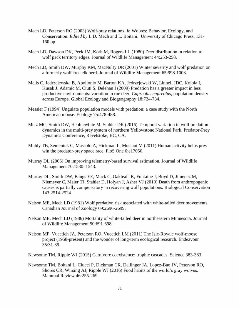
31
Mech LD, Peterson RO (2003) Wolf-prey relations. In Wolves: Behavior, Ecology, and
Conservation. Edited by L.D. Mech and L. Boitani. University of Chicago Press. 131-
160 pp.
Mech LD, Dawson DK, Peek JM, Korb M, Rogers LL (1980) Deer distribution in relation to
wolf pack territory edges. Journal of Wildlife Management 44:253-258.
Mech LD, Smith DW, Murphy KM, MacNulty DR (2001) Winter severity and wolf predation on
a formerly wolf-free elk herd. Journal of Wildlife Management 65:998-1003.
Melis C, Jedrzejewska B, Apollonio M, Barton KA, Jedrzejewski W, Linnell JDC, Kojola I,
Kusak J, Adamic M, Ciuti S, Delehan I (2009) Predation has a greater impact in less
productive environments: variation in roe deer, Capreolus capreolus, population density
across Europe. Global Ecology and Biogeography 18:724-734.
Messier F (1994) Ungulate population models with predation: a case study with the North
American moose. Ecology 75:478-488.
Metz MC, Smith DW, Hebblewhite M, Stahler DR (2016) Temporal variation in wolf predation
dynamics in the multi-prey system of northern Yellowstone National Park. Predator-Prey
Dynamics Conference, Revelstoke, BC, CA.
Muhly TB, Semeniuk C, Massolo A, Hickman L, Musiani M (2011) Human activity helps prey
win the predator-prey space race. PloS One 6:e17050.
Murray DL (2006) On improving telemetry-based survival estimation. Journal of Wildlife
Management 70:1530–1543.
Murray DL, Smith DW, Bangs EE, Mack C, Oakleaf JK, Fontaine J, Boyd D, Jimenez M,
Niemeyer C, Meier TJ, Stahler D, Holyan J, Asher VJ (2010) Death from anthropogenic
causes is partially compensatory in recovering wolf populations. Biological Conservation
143:2514-2524.
Nelson ME, Mech LD (1981) Wolf predation risk associated with white-tailed deer movements.
Canadian Journal of Zoology 69:2696-2699.
Nelson ME, Mech LD (1986) Mortality of white-tailed deer in northeastern Minnesota. Journal
of Wildlife Management 50:691-698.
Nelson MP, Vucetich JA, Peterson RO, Vucetich LM (2011) The Isle-Royale wolf-moose
project (1958-present) and the wonder of long-term ecological research. Endeavour
35:31-39.
Newsome TM, Ripple WJ (2015) Carnivore coexistence: trophic cascades. Science 383-383.
Newsome TM, Boitani L, Ciucci P, Dickman CR, Dellinger JA, Lopez-Bao JV, Peterson RO,
Shores CR, Wirsing AJ, Ripple WJ (2016) Food habits of the world’s gray wolves.
Mammal Review 46:255-269.
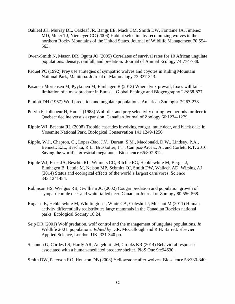
32
Oakleaf JK, Murray DL, Oakleaf JR, Bangs EE, Mack CM, Smith DW, Fontaine JA, Jimenez
MD, Meier TJ, Niemeyer CC (2006) Habitat selection by recolonizing wolves in the
northern Rocky Mountains of the United States. Journal of Wildlife Management 70:554-
563.
Owen-Smith N, Mason DR, Ogutu JO (2005) Correlates of survival rates for 10 African ungulate
populations: density, rainfall, and predation. Journal of Animal Ecology 74:774-788.
Paquet PC (1992) Prey use strategies of sympatric wolves and coyotes in Riding Mountain
National Park, Manitoba. Journal of Mammalogy 73:337-343.
Pasanen-Mortensen M, Pyykonen M, Elmhagen B (2013) Where lynx prevail, foxes will fail –
limitation of a mesopredator in Eurasia. Global Ecology and Biogeography 22:868-877.
Pimlott DH (1967) Wolf predation and ungulate populations. American Zoologist 7:267-278.
Potvin F, Jolicoeur H, Huot J (1988) Wolf diet and prey selectivity during two periods for deer in
Quebec: decline versus expansion. Canadian Journal of Zoology 66:1274-1279.
Ripple WJ, Beschta RL (2008) Trophic cascades involving cougar, mule deer, and black oaks in
Yosemite National Park. Biological Conservation 141:1249-1256.
Ripple, W.J., Chapron, G., Lopez-Bao, J.V., Durant, S.M., Macdonald, D.W., Lindsey, P.A.,
Bennett, E.L., Beschta, R.L., Bruskotter, J.T., Campos-Arceiz, A., and Corlett, R.T. 2016.
Saving the world’s terrestrial megafauna. Bioscience 66:807-812.
Ripple WJ, Estes JA, Beschta RL, Wilmers CC, Ritchie EG, Hebblewhite M, Berger J,
Elmhagen B, Letnic M, Nelson MP, Schmitz OJ, Smith DW, Wallach AD, Wirsing AJ
(2014) Status and ecological effects of the world’s largest carnivores. Science
343:1241484.
Robinson HS, Wielgus RB, Gwilliam JC (2002) Cougar predation and population growth of
sympatric mule deer and white-tailed deer. Canadian Journal of Zoology 80:556-568.
Rogala JK, Hebblewhite M, Whittington J, White CA, Coleshill J, Musiani M (2011) Human
activity differentially redistributes large mammals in the Canadian Rockies national
parks. Ecological Society 16:24.
Seip DR (2001) Wolf predation, wolf control and the management of ungulate populations. In
Wildlife 2001: populations. Edited by D.R. McCullough and R.H. Barrett. Elsevier
Applied Science, London, UK. 331-340 pp.
Shannon G, Cordes LS, Hardy AR, Angeloni LM, Crooks KR (2014) Behavioral responses
associated with a human-mediated predator shelter. PloS One 9:e94630.
Smith DW, Peterson RO, Houston DB (2003) Yellowstone after wolves. Bioscience 53:330-340.
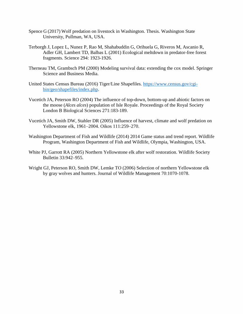
33
Spence G (2017) Wolf predation on livestock in Washington. Thesis. Washington State
University, Pullman, WA, USA.
Terborgh J, Lopez L, Nunez P, Rao M, Shahabuddin G, Orihuela G, Riveros M, Ascanio R,
Adler GH, Lambert TD, Balbas L (2001) Ecological meltdown in predator-free forest
fragments. Science 294: 1923-1926.
Therneau TM, Grambsch PM (2000) Modeling survival data: extending the cox model. Springer
Science and Business Media.
United States Census Bureau (2016) Tiger/Line Shapefiles. https://www.census.gov/cgi-
bin/geo/shapefiles/index.php.
Vucetich JA, Peterson RO (2004) The influence of top-down, bottom-up and abiotic factors on
the moose (Alces alces) population of Isle Royale. Proceedings of the Royal Society
London B Biological Sciences 271:183-189.
Vucetich JA, Smith DW, Stahler DR (2005) Influence of harvest, climate and wolf predation on
Yellowstone elk, 1961–2004. Oikos 111:259–270.
Washington Department of Fish and Wildlife (2014) 2014 Game status and trend report. Wildlife
Program, Washington Department of Fish and Wildlife, Olympia, Washington, USA.
White PJ, Garrott RA (2005) Northern Yellowstone elk after wolf restoration. Wildlife Society
Bulletin 33:942–955.
Wright GJ, Peterson RO, Smith DW, Lemke TO (2006) Selection of northern Yellowstone elk
by gray wolves and hunters. Journal of Wildlife Management 70:1070-1078.
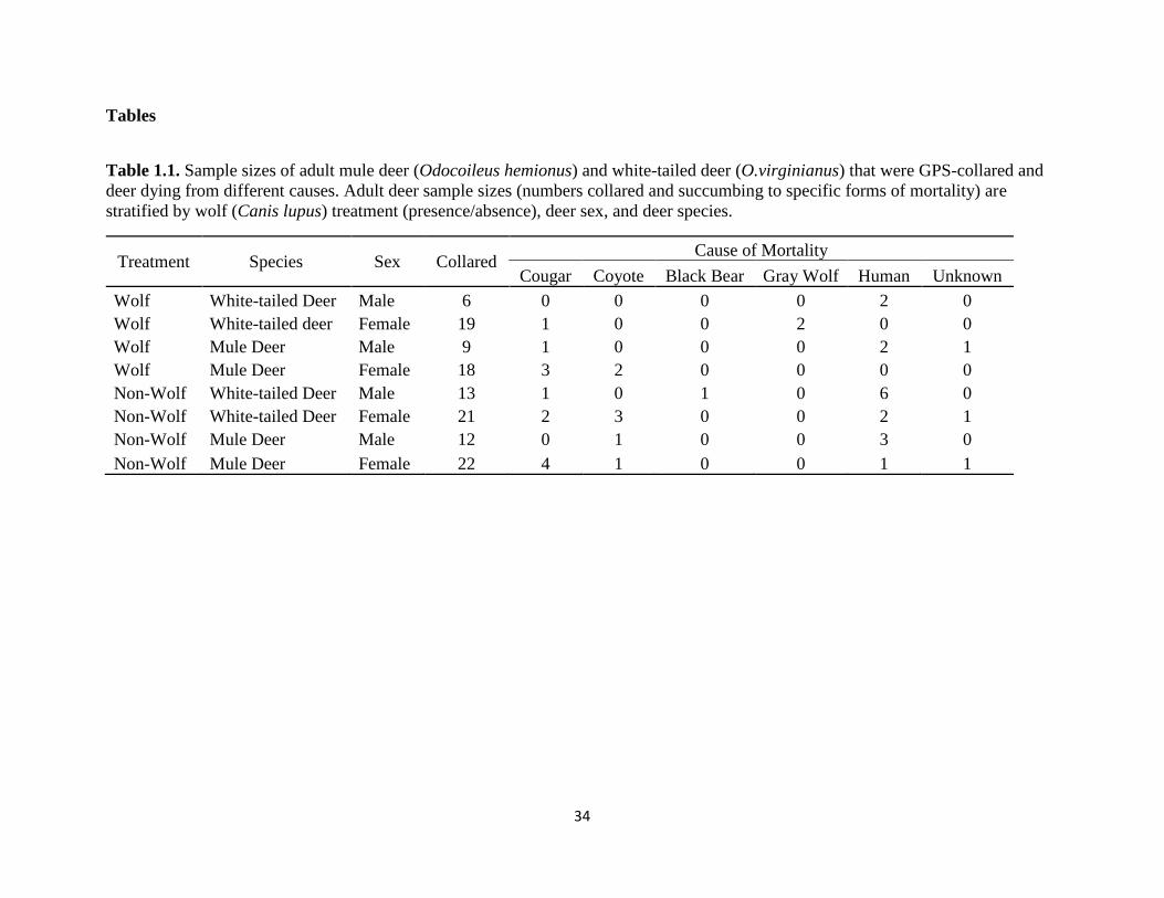
34
Tables
Table 1.1. Sample sizes of adult mule deer (Odocoileus hemionus) and white-tailed deer (O.virginianus) that were GPS-collared and
deer dying from different causes. Adult deer sample sizes (numbers collared and succumbing to specific forms of mortality) are
stratified by wolf (Canis lupus) treatment (presence/absence), deer sex, and deer species.
Treatment Species Sex Collared Cause of Mortality
Cougar Coyote Black Bear Gray Wolf Human Unknown
Wolf White-tailed Deer Male 6 0 0 0 0 2 0
Wolf White-tailed deer Female 19 1 0 0 2 0 0
Wolf Mule Deer Male 9 1 0 0 0 2 1
Wolf Mule Deer Female 18 3 2 0 0 0 0
Non-Wolf White-tailed Deer Male 13 1 0 1 0 6 0
Non-Wolf White-tailed Deer Female 21 2 3 0 0 2 1
Non-Wolf Mule Deer Male 12 0 1 0 0 3 0
Non-Wolf Mule Deer Female 22 4 1 0 0 1 1
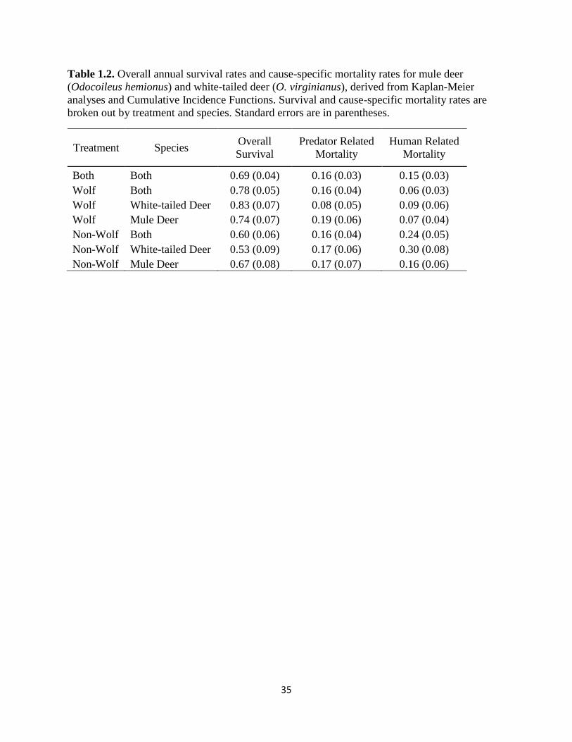
35
Table 1.2. Overall annual survival rates and cause-specific mortality rates for mule deer
(Odocoileus hemionus) and white-tailed deer (O. virginianus), derived from Kaplan-Meier
analyses and Cumulative Incidence Functions. Survival and cause-specific mortality rates are
broken out by treatment and species. Standard errors are in parentheses.
Treatment Species Overall
Survival
Predator Related
Mortality
Human Related
Mortality
Both Both 0.69 (0.04) 0.16 (0.03) 0.15 (0.03)
Wolf Both 0.78 (0.05) 0.16 (0.04) 0.06 (0.03)
Wolf White-tailed Deer 0.83 (0.07) 0.08 (0.05) 0.09 (0.06)
Wolf Mule Deer 0.74 (0.07) 0.19 (0.06) 0.07 (0.04)
Non-Wolf Both 0.60 (0.06) 0.16 (0.04) 0.24 (0.05)
Non-Wolf White-tailed Deer 0.53 (0.09) 0.17 (0.06) 0.30 (0.08)
Non-Wolf Mule Deer 0.67 (0.08) 0.17 (0.07) 0.16 (0.06)
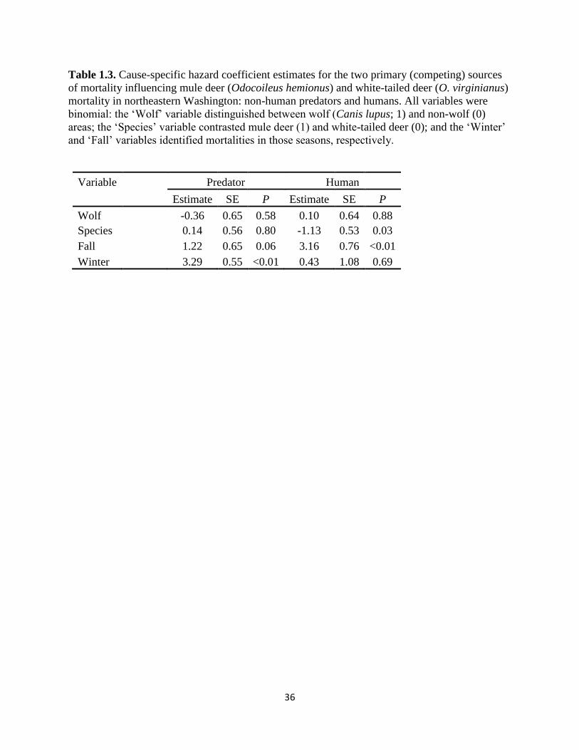
36
Table 1.3. Cause-specific hazard coefficient estimates for the two primary (competing) sources
of mortality influencing mule deer (Odocoileus hemionus) and white-tailed deer (O. virginianus)
mortality in northeastern Washington: non-human predators and humans. All variables were
binomial: the ‘Wolf’ variable distinguished between wolf (Canis lupus; 1) and non-wolf (0)
areas; the ‘Species’ variable contrasted mule deer (1) and white-tailed deer (0); and the ‘Winter’
and ‘Fall’ variables identified mortalities in those seasons, respectively.
Variable Predator Human
Estimate SE P Estimate SE P
Wolf -0.36 0.65 0.58 0.10 0.64 0.88
Species 0.14 0.56 0.80 -1.13 0.53 0.03
Fall 1.22 0.65 0.06 3.16 0.76 <0.01
Winter 3.29 0.55 <0.01 0.43 1.08 0.69
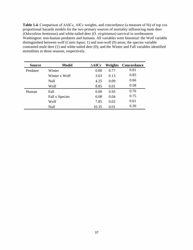
37
Table 1.4. Comparison of ∆AICc, AICc weights, and concordance (a measure of fit) of top cox
proportional hazards models for the two primary sources of mortality influencing mule deer
(Odocoileus hemionus) and white-tailed deer (O. virginianus) survival in northeastern
Washington: non-human predators and humans. All variables were binomial: the Wolf variable
distinguished between wolf (Canis lupus; 1) and non-wolf (0) areas; the species variable
contrasted mule deer (1) and white-tailed deer (0); and the Winter and Fall variables identified
mortalities in those seasons, respectively.
Source Model ∆AICc Weights Concordance
Predator Winter 0.00 0.77 0.81
Winter x Wolf 3.63 0.13 0.85
Null 4.25 0.09 0.66
Wolf 8.85 0.01 0.58
Human Fall 0.00 0.93 0.76
Fall x Species 6.08 0.04 0.75
Wolf 7.85 0.02 0.61
Null 10.35 0.01 0.30
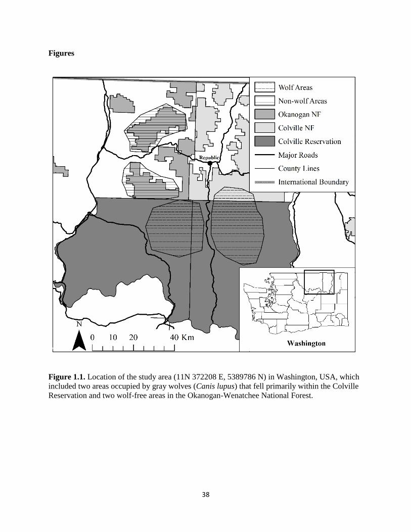
38
Figures
Figure 1.1. Location of the study area (11N 372208 E, 5389786 N) in Washington, USA, which
included two areas occupied by gray wolves (Canis lupus) that fell primarily within the Colville
Reservation and two wolf-free areas in the Okanogan-Wenatchee National Forest.
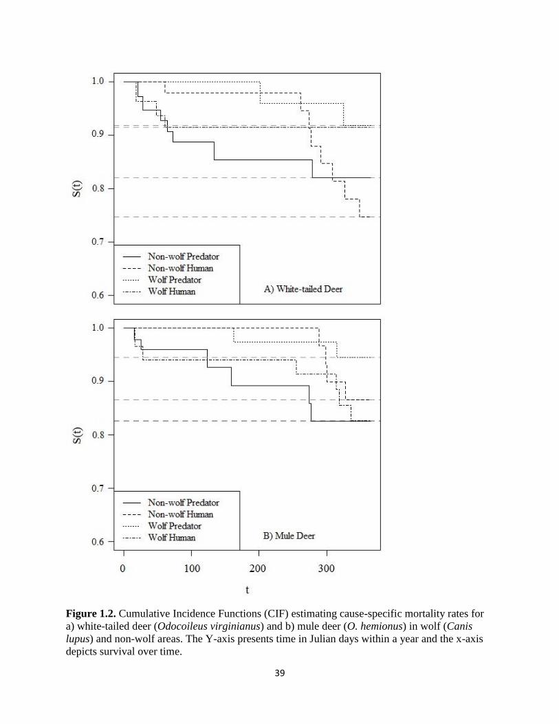
39
Figure 1.2. Cumulative Incidence Functions (CIF) estimating cause-specific mortality rates for
a) white-tailed deer (Odocoileus virginianus) and b) mule deer (O. hemionus) in wolf (Canis
lupus) and non-wolf areas. The Y-axis presents time in Julian days within a year and the x-axis
depicts survival over time.
40
Chapter 2: Escape behavior predicts divergent anti-predator responses of sympatric prey
to recolonizing gray wolves
*In review as: Dellinger JA, Shores CR, Craig A, Heithaus MR, Ripple, WJ, Wirsing AJ. Escape
behavior predicts divergent anti-predator responses of sympatric prey to recolonizing gray
wolves.
Abstract: There is growing appreciation for the role prey escape behavior can play in shaping
non-consumptive effects of predators. We took advantage of ongoing gray wolf recolonization in
eastern Washington, USA to contrast habitat use patterns of two sympatric prey species with
different escape tactics – mule and white-tailed deer – at sites with and without established wolf
packs. Under the hypothesis that the nature and scale of responses by these ungulates to wolf
predation risk hinge on their escape behavior, we predicted that (1) mule deer would avoid
encounters with wolves with coarse-scale spatial shifts to rugged terrain, where their stotting
(bounding) and active-defense escape tactics are most effective; and that (2) white-tailed deer
would not seek to avoid wolves but rather manage wolf risk with fine-scale spatial shifts toward
gentle terrain facilitating their sprinting escape mode. Resource selection functions based on 61
mule deer and 59 white-tailed deer equipped with GPS radio-collars from 2013-2016 revealed
that habitat use patterns for each species were altered by wolf presence, but in divergent ways
that supported our predictions. More broadly, our findings add to a growing literature
highlighting escape behavior as a key driver of contingency in prey responses to predation risk
across multiple ecosystem types and, consequently, suggest that predators could initiate multiple
direct and indirect non-consumptive effects (trophic cascades) in the same ecosystem that are
transmitted by divergent responses of sympatric prey with different escape modes.
41
Introduction
Behavioral responses of prey to predators often take the form of shifts in habitat use,
which in turn may influence how prey exploit resources and interact with co-occurring species
(Lima and Dill 1990; Fortin et al. 2005; Thaker et al. 2011; Latombe et al. 2014). Prey
individuals are typically assumed to avoid their predators (Laundre et al. 2010), diminishing their
ecological effects (e.g., foraging pressure) where predators are more numerous, while increasing
their impacts where predators are relatively scarce (Ripple and Beschta 2012). A growing
literature, however, suggests that prey responses to predators hinge on key features of the
interaction such as predator hunting mode and landscape context and, as a result, that anti-
predator habitat shifts and their consequences will not always follow this pattern (Schmitz 2008;
Heithaus et al. 2009; Wirsing et al. 2010). For example, Schmitz (2008) found that the hunting
mode of sympatric spider predators (sit-and-wait versus active) dictated whether herbivorous
grasshoppers (Melanopuls femurrubrum) foraged in refuge or exposed grassland habitat and, as a
result, promoted either increased or reduced plant diversity. Working in a coral reef ecosystem,
Catano et al. (2016) observed that landscape heterogeneity mediated avoidance of a predator
decoy by herbivorous fishes, with reef complexity apparently enhancing avoidance because it
impedes both predator detection and escape. By implication, efforts to identify the factors that
determine how prey use space when threatened with predation are crucial to the development of
a general framework for predicting the effects of predators on their prey and, ultimately,
ecosystems.
Escape behavior has been proposed as an important driver of context dependence in
predator-prey relationships that interacts with predator hunting mode and landscape features to
determine prey spatial responses to predation risk (Lingle 2002; Heithaus et al. 2009; Wirsing et
42
al. 2010). Overall predation risk can be decomposed into the probability of encountering a
predator (pre-encounter risk) and the probability of death as a result of the encounter (post-
encounter risk) (Lima and Dill 1990; Hebblewhite et al. 2005). Thus, prey individuals with
certain escape tactics might actually benefit from minimizing post-encounter risk by using space
where predators are relatively abundant but less lethal, whereas prey species with escape
behaviors that do not facilitate surviving an encounter with a predator should seek to minimize
pre-encounter risk by avoiding the predator altogether (Heithaus et al. 2009; Wirsing et al. 2010).
In a given ecosystem, the hunting mode of the predator and the structure of the landscape will
determine the spatial pattern of predator lethality experienced by each prey species and,
consequently, which prey species might benefit from managing pre- versus post-encounter risk
(Heithaus et al. 2009; Wirsing et al. 2010). This framework has implications for the spatial scale
at which prey species should respond to the risk of predation. Namely, prey species whose
escape behavior facilitates surviving an encounter should be expected to manifest fine-scale
habitat shifts when exposed to the threat of predation, whereas those seeking to minimize pre-
encounter risk should exhibit coarse-scale shifts in habitat use in response to the predator
(Kauffman et al. 2007). To date, few studies have tested whether escape behavior can predict
contrasting spatial responses of different prey species to a shared predator in the same landscape.
Accordingly, we examined the possibility that recolonizing gray wolves (Canis lupus) in eastern
Washington, USA elicit divergent habitat shifts by two sympatric herbivores – mule deer
(Odocoileus hemionus) and white-tailed deer (O. virginianus) – with different modes of escape.
In 2008, gray wolves began naturally recolonizing Washington from southern British
Columbia, Canada and northern Idaho, and there are now 20 confirmed packs in the state
(Jimenez and Becker 2016). At present, these packs are distributed heterogeneously across
43
eastern Washington, setting the stage for natural experiments examining the effects of gray wolf
recolonization on prey populations, including habitat use patterns, by contrasting areas with and
without resident wolves. In this region, mule deer and white-tailed deer dominate the ungulate
guild (Robinson et al. 2002), and gray wolves are known to primarily consume both species
(making up ≥50% of wolf diet depending on the pack) within this region (Spence 2017). Mule
deer and white-tailed deer may differ in their responses to presence of wolves, however, because
their respective escape tactics are most effective in different habitat types (Lingle and Pellis
2002). Specifically, mule deer stot (i.e., bound) and exhibit active defense, and both of these
escape tactics are facilitated by uneven terrain, especially against coursing canid predators
(Lingle 2002). White-tailed deer, by contrast, are better equipped to escape canids on relatively
gentle terrain because they flee predators and rely on early detection (Lingle and Pellis 2002). As
coursing predators, gray wolves tend to select for relatively gentle terrain while hunting (
Supplementary Material 2.1; Mech and Peterson 2003; Oakleaf et al. 2006). Thus, we might
expect mule deer to exhibit coarse-scale habitat shifts from gentle to rugged terrain that reduce
the likelihood of encounters with gray wolves (i.e., pre-encounter risk) while also promoting
escape in the event of an attack. Conversely, white-tailed deer exposed to wolves should be more
likely to remain in areas dominated by gentle terrain, given the presumed lethality associated
with encountering predators in rugged areas, and exhibit finer-scale shifts in habitat use that
enhance the possibility of escaping a predator encounter.
Here, taking advantage of spatial heterogeneity in wolf presence, we contrasted both
coarse- and fine-scale habitat use patterns of adult mule deer and white-tailed deer in areas with
and without established packs. We hypothesized that the nature and scale of anti-predator
responses of these two deer species to wolves are mediated by escape behavior. Under this
44
hypothesis, we expected mule deer to seek to avoid wolf encounters by increasing their use of
rugged terrain and, consequently, that differences in habitat use patterns of this prey species in
wolf-present and wolf-absent areas would be greatest at a relatively coarse spatial scale (Wirsing
et al. 2010). Specifically, we predicted that, relative to conspecifics in wolf-absent areas, mule
deer in wolf-present areas would exhibit increased use of space: 1) with greater slope (Lingle and
Pellis 2002); 2) farther from roads (due to roads being graded/flatter surfaces that facilitate
coursing movements; Whittington et al. 2011); and 3) closer to cover (i.e., more forested habitat
to avoid detection; Hernandez and Laundre 2005) (Table 1). By contrast, because escape success
of white-tailed deer has been shown to correlate spatially with terrain that is typically hunted by
wolves, we predicted that differences in habitat use patterns of this prey species in wolf-present
and wolf-absent areas would be greatest at relatively fine spatial scales (Heithaus et al. 2009;
Wirsing et al. 2010). Specifically, we predicted that, relative to conspecifics in wolf-absent areas,
white-tailed deer in wolf-present areas would show increased use of space: 1) with reduced slope
(Lingle and Pellis 2002); 2) closer to roads (fewer obstacles on roads to inhibit escape; Kunkel
and Pletscher 2001); and 3) farther from cover (i.e., more open shrub habitat to aid in early
detection; Kittle et al. 2008; Table 1).
Materials and methods
Study area
This study took place from 2013-2016 in an area of eastern Washington spanning
Okanogan and Ferry Counties and including portions of the Okanogan-Wenatchee and Colville
National Forests and the Colville Reservation (Fig. 2.1). The study area contains the Okanogan
Highlands and Kettle River Range. These areas are composed of similar topography with
45
predominantly moderate slopes on mountainous and hilly terrain (Supplementary Material 2.2).
The Sanpoil River is the main drainage that bisects the Okanogan Highlands and Kettle River
Range. Elevation in the area ranges from 300 to 2,065 m. Shrub steppe habitats composed
primarily of sagebrush (Artemisia tridentata) and bitterbrush (Purshia tridentata) makeup most
of the habitat at lower elevations, whereas ponderosa pine (Pinus ponderosa), Douglas-fir
(Pseudotsuga menziesii), and subalpine fir (Abies lasiocarpa) forest dominate at higher
elevations. Riparian areas, composed primarily of poplars (Populus spp.), are regularly dispersed
along drainages (Clausnitzer and Zamora 1987). Mule deer, white-tailed deer, elk (Cervus
elaphus), and moose (Alces alces) comprise the resident ungulate community, though each deer
species is 20 and 50 times more abundant than moose and elk, respectively (Spence 2017).
Coyotes (Canis latrans), bobcats (Lynx rufus), American black bears (Ursus americanus), and
cougars (Puma concolor) represent the larger mammalian predators present throughout the study
area.
We broke the study area into four separate sites, two occupied by gray wolf packs and
two lacking wolves. The four sites encompassed an average of 613 km2 (range = 550-680 km2).
In areas of Washington that have been recolonized by gray wolves, average home range size,
average pack size, and pack density are similar to those documented in other managed
landscapes in neighboring states (Jimenez and Becker 2016), but pack size and pack density in
all of these managed areas are low relative to protected areas (Jimenez and Becker 2016). Wolf
packs were first detected in the region in the summer of 2010 and, over the course of the
investigation, were found to occupy the Colville National Forest and Colville Reservation but not
the adjacent Okanogan-Wenatchee National Forest (Fig. 2.1). Specifically, wolf-present areas
were situated immediately east (Nc’icn Pack) and west (Strawberry Pack) of the Sanpoil River

46
and State Highway 21. One wolf-absent site, named ‘Aeneas’, was immediately south of Aeneas
Valley and State Highway 20, and north of the Colville Reservation. The other wolf-absent site,
named ‘Bonaparte’, was located near Bonaparte Lake and north of State Highway 20 (Fig. 2.1).
No site was more than 30 km from the three other sites. All four sites experience similar levels of
human use in the form of cattle ranching, logging, and hunting. Cattle grazed freely on the
landscape in each year of the investigation from approximately mid-June to mid-October.
Logging occurred year round with variable harvest intensity and cut block size. Hunting of both
deer species on the National Forests occurs in autumn and length of season varies depending on
Game Management Unit (GMU) and weapon-type. Generally, no GMU is hunted more than two
full months in a year during autumn. Both wolf-absent areas primarily occurred in GMU 204.
Hunting of both species on the Colville Reservation primarily occurs during the autumn months.
Data Collection
We monitored gray wolf activity in all four sites within the study area in three ways. First, we
deployed sixteen motion-activated game cameras (M880 by Moultrie®, Calera, AL, USA) year
round as a grid (1 per 5 km2) along logging roads and game trails at each site, and checked the
cameras every three months. Second, we conducted weekly track surveys at each study site along
logging roads and game trails during winter months (mid-December to mid-March) using
snowmobiles. Third, radio-collars deployed on at least two members of each wolf pack
occupying the designated wolf areas by the Colville Confederated Tribes Fish and Wildlife
Department aided in monitoring wolf presence, movements, and pack size. Combined, these
three methods enabled continuous and intensive monitoring of occupancy and overall number of
wolves present in each site. Neither wolf-absent site had any documented gray wolf activity
47
during the course of this study, whereas both of the wolf-present sites were occupied by packs
ranging in size from 3-8 individuals over the course of the investigation.
To determine habitat use patterns of mule and white-tailed deer, we captured individuals
of each species over three consecutive winters (December – March) using aerial net gunning and
baited clover trapping (Haulton et al. 2001). We outfitted clover traps with trap transmitters to
alert us to captures. Trap transmitter signals were checked daily in the early morning and late
afternoon. Captured deer were equipped with Global Positioning System (GPS) radio-collars
(Globalstar Survey Collars, Vectronic Aerospace Gmbh, Berlin, Germany), ear tagged, aged,
sexed, and weighed. To ensure that only adults were collared, we did not instrument any
individual weighing < 30 kg (Haulton et al. 2001). The GPS collars were programmed to obtain a
location every 12 hours and five minutes, in the interest of obtaining an even distribution of
locations throughout the day, and to switch to mortality mode if the instrumented deer exhibited
no movement for a 24-hour period. All animal captures and collar deployments were conducted
under University of Washington Institutional Animal Care and Use Committee (IACUC)
protocol number 4226-01 and wildlife collection permits from the Washington Department of
Fish and Wildlife and the Colville Tribes Fish and Wildlife Department.
Analyses
We used GPS data from radio-collared mule deer and white-tailed deer to examine
patterns of resource use with a use-availability framework that compared landscape attributes
associated with used locations to those at regularly generated available locations (Benson 2013).
We analyzed resource use at two spatial scales. First, we created a 95% minimum convex
polygon (MCP) home range estimate for each radio-collared deer. Regularly spaced points

48
occurring every 30 m (minimum pixel size of spatial data used in analyses) within each 95%
MCP home range served as used locations. Then we created a 95% MCP encompassing all deer
GPS locations to represent available habitat for a second-order resource use analysis examining
the drivers of home range establishment across the landscape by mule and white-tailed (Johnson
1980). Regularly spaced points occurring every 30 m within the study area, but not within
individual deer home ranges, served as available locations for this coarse-scale analysis (Johnson
1980; Benson 2013). We then compared regularly spaced points within individual deer home
ranges to regularly spaced points within the study area to quantify any differences in home range
establishment (i.e., coarse-scale habitat use) for both deer species in wolf-present and wolf-
absent areas. Second, we used the 95% MCP home range estimates for each radio-collared deer
above as the basis for a third-order resource use analysis that explored drivers of space use
within the home range (Johnson 1980). Regularly spaced points occurring every 30 m within
each individual deer home range served as available locations for this relatively fine-scale habitat
use analysis (Johnson 1980; Benson 2013). We then compared GPS fix locations to available
locations within each individual home range to determine differences in resource use patterns of
both deer species in wolf-present and wolf-absent areas at a fine spatial scale. We developed
resource selection functions (RSFs) for both deer species, at both spatial scales, by estimating
coefficients for landscape attributes from a binomial logistic regression of used versus available
locations (Manly et al. 2002; Johnson et al. 2006). We accounted for the influence of GPS fix
success on RSF estimates by including weights for detection depending on habitat type (Nielson
et al. 2009). We included a random effect for individual in the model building process to account
for among-individual variance in habitat use patterns that we could not specifically address with
fixed effects. RSFs resulting from this approach yield coefficient estimates that can be used to
49
understand relative probability of use of areas along a gradient of habitat attributes for species of
interest (Boyce et al. 2002).
We included the following landscape attributes as explanatory variables in the global
RSFs (i.e., the base models from which the above predictions were tested) for each deer species
and spatial scale combination (four total): 1) distance to habitat type in meters (forest and shrub);
2) landscape attributes (slope and distance to nearest road); 3) wolf presence/absence; and 4)
season. We classified season by noting the date of each GPS location and then using binary
coding (0/1), with winter (October – March) set as the reference season (0). Binary classification
of season allowed for simplistic representation of snow presence (present versus absent) on the
landscape. Wolf presence was also expressed as a binary effect (0/1), whereby radio-collared
deer in areas without wolves present served as the reference treatment. We included a two-way
interaction between wolf and season to investigate differences in deer behavior among various
combinations of treatment (wolf-present and wolf-absent) and season (summer and winter). We
also included two-way interactions between wolf and season, respectively, and each other
variable (habitat types and landscape attributes). If deer in wolf-present and wolf-absent areas
behaved divergently, then both the binary wolf presence/absence variable and at least one of the
two-way interactions including the wolf variable would be significant. Furthermore, we included
three-way interactions involving wolf presence/absence, season, and each other variable. These
three-way interactions allowed for discerning potential differences in habitat use between mule
deer and white-tailed deer as a function of various combinations of treatment (wolf-present and
wolf-absent) and season (summer and winter). We obtained raw data for habitat types from the
Washington GAP (Geospatial Analysis Project) raster habitat layer (United States Geological
Survey 2011), and for secondary roads and landscape attributes from the Washington State GIS
50
data clearinghouse (https://wagda.lib.washington.edu/data/geography/wa_state/; accessed
11/15/2016). We analyzed all spatial data at a 30 x 30 m resolution. We assessed habitat type and
landscape attributes using a Euclidean Distance Analysis (EDA) framework (Benson 2013).
Briefly, we estimated the straight-line distance from each pixel (at 30 x 30 m resolution) to the
nearest secondary road, forest cover, or shrub habitat. We then standardized these EDA distance
values by subtracting each value by the mean and then dividing by the standard deviation to
render coefficient estimates derived from these variables easier to interpret (Benson 2013).
Initially, we also included deer sex for both ungulate species as a fixed effect in our RSFs.
However, preliminary analyses revealed little effect of sex on differences in habitat use patterns
between deer of either species in wolf-present and wolf-absent areas and between seasons at
either spatial scale. Accordingly, in order to maximize sample size, we pooled the sexes in
subsequent models (Table 2). We assessed performance of RSFs using cross-validation
procedures (Supplementary Material 2.3; Johnson et al. 2006; Benson 2013; Dellinger et al.
2013).
We used Program R version 3.1.2 (R Core Team, 2014) for all statistical analyses, and
ArcView GIS version 10.2 Geographic Information System (GIS; ESRI, Redlands, California)
and Geospatial Modeling Environment version 0.7.4.0 (Beyer 2015) for spatial analyses. In all
analyses, we considered P ≤ 0.05 to be statistically significant.
Results
Across our four study sites over the course of three years, we collared 120 adult deer (n =
61 mule deer, n = 59 white-tailed deer; Table 2). We collected an average of 700 locations (±
51
562 sd) per radio-collared individual, with an average successful GPS fix rate of 81% (75-88%).
Individuals were monitored for an average of 433 days (± 275 sd).
Overall, model-averaged coefficient estimates for mule deer demonstrated greater
disparity in resource use patterns as a function of wolf presence at a coarse spatial scale (i.e.,
with respect to second-order resource use; Table 3; Fig. 2). Furthermore, differences in use of
particular resources by mule deer in wolf-present and wolf-absent areas generally supported the
prediction that this species would manage wolf predation risk with habitat shifts that facilitate
encounter avoidance (Tables 1, 3). Specifically, relative to conspecifics in wolf-absent areas,
mule deer in wolf-present areas exhibited (i) a lower probability of using areas close to
secondary roads at the coarse-scale of analysis; (ii) a lower probability of using areas with low
slope at the coarse-scale; and (iii) a higher probability of using areas close to forested habitat at
the coarse-scale. Mule deer in wolf-present and wolf-absent areas selected shrub habitat in a
similar manner at both coarse and fine spatial scales. Mule deer exhibited some seasonality in
habitat use patterns at the coarse-scale. Namely, use of space relative to roads varied between
seasons, with mule deer manifesting increased use of areas close to roads in wolf-absent areas
during winter and the opposite pattern in the wolf-present areas. Furthermore, at the coarse-scale
mule deer in wolf-present areas selected for forest more in winter compared to summer. Fine-
scale habitat use patterns of mule deer in wolf-present versus wolf-absent areas were more
similar in summer than in winter. For example, mule deer in wolf-present areas more readily
avoided areas as distance to forest and shrub cover increased, respectively, compared to mule
deer in wolf-absent areas during winter (Fig. 2).
Overall, model-averaged coefficient estimates of white-tailed deer demonstrated greater
disparity in resource use patterns as a function of wolf presence at a relatively fine spatial scale
52
(i.e., with respect to third-order resource use; Table 3; Fig. 3). Moreover, differences in use of
particular resources by white-tailed deer in wolf-present and wolf-absent areas generally
supported the prediction that this species would manage predation risk from wolves with habitat
shifts that facilitate post-encounter escape (Table 1, 3). Specifically, relative to conspecifics in
wolf-absent areas, white-tailed deer in wolf-present areas exhibited (i) a higher probability of
using areas close to secondary roads at the fine spatial scale of analysis; (ii) a higher probability
of using areas with low slope at the fine spatial scale; and (iii) a higher probability of using areas
close to shrub habitat at the fine spatial scale. White-tailed deer in wolf-present and wolf-absent
areas selected forested habitat similarly at both the coarse and fine spatial scales of analysis.
White-tailed deer exhibited some seasonality in habitat use patterns. Namely, in all study areas
white-tailed deer selected areas with lower slope in summer compared to winter at the fine
spatial scale. Coarse-scale habitat use patterns of white-tailed deer in wolf-present areas versus
white-tailed deer in wolf-absent areas were more similar in summer than in winter (Fig. 2). For
example, at the coarse spatial scale white-tailed deer in wolf-present areas responded more to
increasing distance from shrub cover during winter relative to summer compared to conspecifics
in wolf-absent areas (Fig. 3). Cross-validation of model-averaged coefficient estimates revealed
good predictive ability of resource use by mule and white-tailed deer at both coarse and fine
spatial scales (Supplementary Material 2.3).
Discussion
There is now broad agreement that predators can influence prey populations and
community dynamics by eliciting anti-predator behavior (Lima 2002; Hernandez and Laundre
2005; Creel and Christianson 2008). Yet, predicting the responses of prey to particular predators,
and by extension the nature of non-consumptive predator indirect effects in communities,

53
remains a challenge (Heithaus et al. 2009). Predator recolonization events set the stage for
natural experiments that contrast responses of sympatric prey in areas with and without the
returning predator and thereby allow examination of the factors driving divergent anti-predator
responses both within and among prey species (Wirsing et al. 2010; Dorresteijn et al. 2015).
Taking advantage of the return of grey wolves to a multi-prey landscape in eastern Washington,
USA, we found support for the hypothesis that the nature and scale of prey responses to
predation risk are mediated by escape behavior. Specifically, mule deer at risk from wolves
exhibited coarse-scale spatial shifts that suited their escape tactic (stotting) and resulted in wolf
avoidance, whereas white-tailed deer manifested fine-scale shifts that facilitated their escape
mode (sprinting) but resulted in spatial overlap with wolves. Our results offer new insights into
the way these ungulates manage their risk of predation from wolves both spatially and
temporally. More broadly, they validate the use of escape behavior in conjunction with predator
hunting mode and landscape structure to predict prey responses to predation risk (Heithaus et al.
2009; Wirsing et al. 2010) and suggest that predators with certain hunting modes could trigger
multiple indirect non-consumptive effects in the same ecosystem owing to divergent responses of
sympatric prey with different escape tactics.
Mule deer exhibit active defense and stotting as anti-predator behaviors (Lingle 2002),
both of which are fostered by sloped, uneven terrain with obstacles (Lingle and Pellis 2002).
Namely, obstacles and broken ground can reduce angles of attack, in-turn helping to focus
defensive behavior, and favor bounding over running around impediments to movement for
quickly and efficiently covering ground (Lingle 2002). Given that the anti-predator behaviors of
mule deer putatively inhibit escaping wolves in areas that these canids frequent (i.e., areas with
gentle and rolling terrain), we predicted that this prey species would avoid encounters with and
54
reduce the probability of being detected by wolves (Atwood et al. 2009; Wirsing and Ripple
2011) by manifesting coarse-scale shifts toward more rugged uplands with increased slopes (i.e.,
uneven ground; Wirsing et al. 2010; Whittington et al. 2011; Table 1). In accord with this
prediction, differences in resource use by mule deer were best captured by the coarse-scale
analysis, and individuals exhibited patterns of use that are consistent with encounter avoidance.
Specifically, when exposed to wolf predation risk, mule deer shifted into forest cover where
detection by cursorial predators like wolves was less likely (Fortin et al. 2005). Mule deer at risk
from wolves also avoided areas with gentle terrain, which wolves use heavily for hunting (Mech
and Peterson 2003; Oakleaf et al. 2006), and roads and trails, which wolves often use as travel
routes (Supplementary Material 2.1; Kunkel and Pletscher 2001). We also predicted that at the
coarse-scale mule deer in wolf-present areas would avoid areas close to shrub habitat to a greater
extent than conspecifics in wolf-absent areas because shrub habitat facilitates being detected by
wolves. We found, however, that mule deer in wolf-present areas showed no significant
difference in use of areas close to shrub habitat compared to mule deer in wolf-absent areas,
perhaps indicating the foraging benefits of shrub habitat for mule deer (Pierce et al. 2004).
Nevertheless, our results overall are strikingly consistent with the idea that mule deer anti-
predator responses to wolves are governed by their escape mode. In accord with our study,
Lingle (2002) found that mule deer at risk from coyotes on the Alberta prairie responded by
shifting to rugged terrain, and Bowyer (1987) suggested that mule deer fawns select steeper
slopes to avoid coyotes. Notably, however, all of these studies were conducted in areas
characterized by topographical complexity. Accordingly, the manner in which mule deer respond
to the threat of predation from coursing canids in areas with less topographical variation remains
to be determined. We also recognize that mule deer use of more gentle terrain and areas closer to
55
roads in the non-wolf areas relative to the wolf areas may be an attempt to decrease predation
risk from cougars (Pierce et al. 2004), whereas the habitat use pattern we observed in the wolf
areas could reflect risk from both predators (Atwood et al. 2009). We were unable to explore
these possibilities, underscoring the value of future studies capable of discriminating between the
effects of these two predators on mule deer.
White-tailed deer use flight and early detection as anti-predator tactics (Lingle 2002), and
both of these countermeasures are generally facilitated by gentle, open terrain with good
visibility and few obstacles (Lingle and Pellis 2002). Given that the anti-predator behaviors of
white-tailed deer actually promote escaping wolves in areas where wolves hunt, we predicted
that this species would not avoid wolves but rather exhibit fine-scale shifts facilitating running
and vigilance (Wirsing et al. 2010; Wirsing and Ripple 2011; Table 1). In accord with this
prediction, differences in resource use by white-tailed deer were best captured by the fine-scale
analysis (Kuijper et al. 2015), and individuals exhibited patterns of use that are consistent with
facilitating post-encounter escape (Lingle 2002). Namely, white-tailed deer at risk from wolves
selected areas close to roads, which in our study area bisect relatively flat areas with few
obstacles to hinder escape, areas with little to no slope (i.e., areas characterized by level ground
that facilitate sprinting), and more open habitats offering greater visibility. (Kunkel and Pletscher
2001; Lingle and Pellis 2002). Our results agree with previous research suggesting that white-
tailed deer minimize predation risk from coursing predators by relying on early detection, which
is facilitated by use of open habitats and avoidance of dense cover (e.g., Kunkel and Pletscher
2001). They are also consistent with work by Kittle et al. (2008), who found that white-tailed
deer in Ontario, Canada selected for sheltered deer yards with low snowfall in winter that placed
them in close proximity to hunting wolves, and with previous studies demonstrating that,

56
following detection, white-tailed deer are more vulnerable to coursing predators where escape is
impeded by obstacles (e.g., deep snow) or not facilitated via use of roads or established trails
(Nelson and Mech 1991). Collectively, these investigations support the notion that, rather than
avoiding canids like mule deer, white-tailed deer at risk from these coursing predators select
resources that promote their sprinting mode of escape.
Mule deer and white-tailed deer in areas with wolves exhibited greater seasonality in
resource use patterns at the predicted spatial scales of their responses to wolves than conspecifics
in areas without wolves. Specifically, at the coarse-scale mule deer in wolf-present areas had a
higher probability of selecting areas close to forest cover in winter versus summer (Table 1; Fig.
2). This pattern might be the result of adult mule deer making more of an effort to avoid
encounters with wolves in winter, the season during which cervid vulnerability to predation tends
to be greatest (Nelson and Mech 1991). At the fine-scale, white-tailed deer in wolf areas showed
a higher probability of selecting areas close to open shrub in winter versus summer, possibly as a
means of more efficiently detecting and escaping wolves during the most dangerous time of year.
Adult white-tailed deer and mule deer in other systems have been found to exhibit seasonal
differences in habitat use patterns in relation to predation risk, most notably in response to
hunting whereby both deer species selected for cover to decrease detection by human hunters
(Swenson 1982; Kilgo et al. 1998). To date, however, seasonal differences in habitat use patterns
of either species in relation to non-human predation risk remain largely unexplored. Our results
highlight the seasonality that can characterize mule and white-tailed deer responses to wolves
and, by extension, imply that studies with limited temporal scope may underestimate or miss
effects of predators on these ungulates. More broadly, they show that consideration of
spatiotemporal patterning can strengthen insights into predator-prey interactions by revealing
57
context specific processes that influence how prey behaviorally manage predation risk (Padie et
al. 2015).
The conceptual framework underlying this study was originally developed as a result
cross-fertilization of research in aquatic and terrestrial environments (Lima 2002; Heithaus et al.
2009; Wirsing et al. 2010) and then invoked in a marine ecosystem (Heithaus et al. 2012; Catano
et al. 2016). Our findings add to a growing literature (e.g., Crowell et al. 2016; Martin and
Owen-Smith 2016) showing that it also applies in terrestrial settings. Accordingly, they
underscore the value, irrespective of eco-domain, of considering the three-way interaction
between prey escape behavior, predator hunting mode, and landscape structure when predicting
or explaining prey responses to predation risk. For example, large roving predators such as gray
wolves (Middleton et al. 2013) and African wild dogs (Lycaon pictus; Thaker et al. 2011) have
been posited as having weak non-consumptive impacts on prey relative to ambush predators
because their spatially diffuse risk signature minimizes the effectiveness of anti-predator
behaviors such as habitat shifts. Other studies, however, have found that roving predators can
influence prey behavior to a greater extent than their ambushing counterparts (e.g., Creel et al.
2014). Insofar as they bear out predictions from the aforementioned framework, our findings
suggest that this disparity likely owes to context dependence. That is, rather than exerting
uniformly weak non-consumptive effects, roving predators like wolves may elicit marked
behavioral changes when and where the setting allows members of prey species with certain
escape tactics the scope to manage their risk. More broadly, our results suggest that at least some
aspects of predator-prey interactions in aquatic and terrestrial systems operate under a similar set
of ecological ‘rules’, the recognition of which could foster a more general understanding of
58
predator-prey interactions that encompasses a diversity of systems and taxa (Terborgh and Estes
2010; Wirsing and Ripple 2011; Wirsing et al. 2014).
A growing literature suggests that the effects of top predators can be attenuated in
human-dominated ecosystems (Hebblewhite et al. 2005; Gervasi et al. 2013; Ripple et al. 2014;
Kuijper et al. 2016). Indeed, we found that wolves in our study system, where human activity is
pervasive, had weak effects on survival of adult mule and white-tailed deer (Chapter 1). Yet,
here we detected marked behavioral responses in both deer species to recolonizing wolves. By
implication, wolves in our human-managed system might not be numerous enough to kill many
prey individuals (Jimenez and Becker 2016), but their presence may still be sufficient to cause
prey to invest in defensive behavior. Microcosm experiments with invertebrate predator-prey
systems have demonstrated that even when the ability of predators to consume prey is removed
(i.e., consumptive effects equal zero), prey may maintain defensive countermeasures similar
those exhibited by conspecifics exposed to predators capable of killing them (Schmitz et al.
1997; Nelson et al. 2004). Building on these small-scale experiments, our findings add support to
the idea that non-consumptive predator effects can operate even when direct predation is
negligible (Schmitz et al. 1997; Nelson et al. 2004; Creel and Christianson 2008). Our results are
also relevant to the debate over whether recolonizing predators can trigger cascading effects to
lower trophic levels by imposing risk in managed landscapes (Hebblewhite et al. 2005; Gervasi
et al. 2013; Dorresteijn et al. 2015; Kuijper et al. 2016). The mule and white-tailed deer anti-
predator responses we observed mean that wolves have the potential to exert behavior-mediated
indirect effects on plant communities in our system. There remains need, however, for studies
asking whether these responses are strong enough to affect lower trophic levels and examining
the possibility that the effects of wolves on deer in managed landscapes could be superseded in
59
some circumstances by risk effects imposed by human predators (Lone et al. 2014; Dorresteijn et
al. 2015).
In conclusion, our results demonstrate that escape behavior influences the nature and
spatial scale of prey responses to predation risk and thereby highlight the potential for top
predators to impact multiple sympatric prey species at varying spatial scales via risk effects
because of differences in prey escape behavior (Latombe et al. 2014; Padie et al. 2015; Catano et
al. 2016; Makin et al. 2017). By implication, top predators could trigger multiple indirect non-
consumptive effects in the same ecosystem by inducing divergent responses of sympatric prey
with different escape tactics (Wirsing et al. 2010). Accordingly, we encourage further
exploration of direct and indirect effects of predators with shared prey that exhibit divergent
escape behavior in the interest of better understanding the non-consumptive pathways by which
top-down forcing can occur in ecosystems. Given that prey escape responses can depend on
predator hunting mode and landscape context (Lingle 2002; Heithaus et al. 2009; Wirsing et al.
2010; Latombe et al. 2014), studies in systems with multiple predator and prey species
interacting across heterogeneous landscapes are likely to be especially revealing. Finally, from a
conservation standpoint our findings emphasize the important roles played by predators in all
landscapes rather than just protected areas (Heithaus et al. 2012; Dorresteijn et al. 2015; Kuijper
et al. 2016). In particular, our results suggest that even if predators do not inflict much mortality
in human-modified ecosystems, their recovery might at least partly restore key processes such as
defensive investment by prey species (Kuijper et al. 2016) with the potential to generate multiple
trophic cascades (Ripple and Beschta 2012).
60
Literature Cited
Atwood TC, Gese EM, Kunkel KE (2009) Spatial partitioning of predation risk in a multiple
predator-multiple prey system. Journal of Wildlife Management 73:876-884.
Benson JF (2013) Improving rigour and efficiency of use-availability habitat selection analyses
with systematic estimation of availability. Methods in Ecology and Evolution 4:244-251.
Beyer HL (2015) Geospatial Modelling Environment (Version 0.7.4.0). URL:
http://www.spatialecology.com/gme.
Bowyer RT (1987) Coyote group size relative to predation on mule deer. Mammalia 51:515-526.
Boyce MS, Vernier PR, Nielsen SE, Schmiegelow FK (2002) Evaluating resource selection
functions. Ecological Modelling 157:281-300.
Catano LB, Rojas MC, Malossi RJ, Peters JR, Heithaus MR, Fourqurean JW, Burkepile DE
(2016) Reefscapes of fear: predation risk and reef hetero-geneity interact to shape
herbivore foraging behavior. Journal of Animal Ecology 85:146-156.
Clausnitzer RR, Zamora BA (1987) Forest Habitat Types of the Colville Indian Reservation.
Department of Forestry and Range Management, Washington State University, Pullman,
Washington, USA.
Creel S, Christianson D (2008) Relationships between direct predation and risk effects. Trends in
Ecology and Evolution 23:194-201.
Creel S, Schutte P, Christianson D (2014) Effects of predation risk on group size, vigilance, and
foraging behavior in an African ungulate community. Behavioral Ecology 25:773-784.
Crowell MM, Shipley LA, Camp MJ, Rachlow JL, Forbey JS, Johnson TR (2016) Selection of
food patches by sympatric herbivores in response to concealment and distance from a
refuge. Ecology and Evolution 6:2865-2876.
Dellinger JA, Proctor C, Steury TD, Kelly MJ, Vaughan MR (2013) Habitat selection of a large
carnivore, the red wolf, in a human-altered landscape. Biological Conservation 157:324-
330.
Dorresteijn I, Schultner J, Nimmo DG, Fischer J, Hanspach J, Kuemmerle T, Kehoe L, Ritchie
EG (2015) Incorporating anthropogenic effects into trophic ecology: predator-prey
interactions in a human-dominated landscape. Proceedings of the Royal Society B
282:20151602.
Fortin D, Beyer HL, Boyce MS, Smith DW, Duchesne T, Mao JS (2005) Wolves influence elk
movements: behavior shapes a trophic cascade in Yellowstone National Park. Ecology
86:1320-1330.

61
Gervasi V, Sand H, Zimmermann B, Mattisson J, Wabakken P, Linnell JDC (2013)
Decomposing risk: landscape structure and wolf behavior generate different predation
patterns in two sympatric ungulates. Ecological Applications 23:1722-1734.
Haulton SM, Porter WF, Rudolph BA (2001) Evaluating 4 methods to capture white-tailed deer.
Wildlife Society Bulletin 29:255-264.
Hebblewhite M, Merrill EH, McDonald TL (2005) Spatial decomposition of predation risk using
resource selection functions: an example in a wolf-elk predator-prey system. Oikos
111:101-111.
Heithaus MR, Wirsing AJ, Dill LM (2012) The ecological importance of intact top-predator
populations: a synthesis of 15 years of research in a seagrass ecosystem. Marine and
Freshwater Research 63:1039-1050.
Heithaus MR, Wirsing AJ, Burkholder D, Thomson J, Dill LM (2009) Towards a predictive
framework for predator risk effects: the interaction of landscape features and prey escape
tactics. Journal of Animal Ecology 78:556-562.
Hernandez L, Laundre JW (2005) Foraging in the landscape of fear and its implications for
habitat use and diet quality of elk Cervus elaphus and bison Bison bison. Wildlife
Biology 11:215-220.
Jimenez MD, Becker SA (2016) Northern Rocky Mountain Wolf Recovery Program 2015
Interagency Annual Report. U.S. Fish and Wildlife Service, Ecological Services, 585
Shepard Way, Helena, Montana, 59601.
Johnson CJ, Nielsen SE, Merrill EH, McDonald TL, Boyce MS (2006) Resource selection
functions based on use-availability data: theoretical motivation and evaluation methods.
Journal of Wildlife Management 70:347-357.
Johnson DH (1980) The comparison of usage and availability measurements for evaluating
resource preference. Ecology 61:65-71.
Kauffman MJ, Varley N, Smith DW, Stahler DR, MacNulty DR, Boyce MS (2007) Landscape
heterogeneity shapes predation in a newly restored predator-prey system. Ecology Letters
10:690-700.
Kilgo JC, Labisky RF, Fritzen DE (1998) Influences of hunting on the behavior of white-tailed
deer: implications for conservation of the Florida panther. Conservation Biology
12:1359-1364.
Kittle AM, Fryxell JM, Desy GE, Hamr J (2008) The scale-dependent impact of wolf predation
risk on resource selection by three sympatric ungulates. Oecologia 157:163-175.
Kuijper DPJ, Sahlen E, Elmhagen B, Chamaille-Jammes S, Sand H, Lone K, Cromsigt JPGM
(2016) Paws without claws? Ecological effects of large carnivores in anthropogenic
landscapes. Proceedings of the Royal Society B 283:1625
62
Kuijper DPJ, Bubnicki JW, Churski M, Mols B, Van Hooft P (2015) Context dependence of risk
effects: wolves and tree logs create patches of fear in an old-growth forest. Behavioral
Ecology 26:1558-1568.
Kunkel K, Pletscher DH (2001) Winter hunting patterns of wolves in and near Glacier National
Park, Montana. Journal of Wildlife Management 65:520-530.
Latombe G, Fortin D, Parrott L (2014) Spatio-temporal dynamics in the response of woodland
caribou and moose to the passage of grey wolf. Journal of Animal Ecology 83:185-198.
Laundré JW, Hernández L, Ripple WJ (2010) The landscape of fear: ecological implications of
being afraid. Open Ecology J 3:1-7.
Lima SL (2002) Putting predators back into behavioral predator-prey interactions. Trends in
Ecology and Evolution 17:70-75.
Lima SL, Dill LM (1990) Behavioral decisions made under the risk of predation: a review and
prospectus. Canadian Journal of Zoology 68:619-640.
Lingle S (2002) Coyote predation and habitat segregation of white-tailed deer and mule deer.
Ecology 83:2037-2048.
Lingle S, Pellis S (2002) Fight or flight? Antipredator behavior and the escalation of coyote
encounters with deer. Oecologia 131:154-164.
Manly BFJ, McDonald LL, Thomas DL, McDonald TL, Erickson WP (2002) Resource selection
by animals: statistical analysis and design for field studies. 2nd ed., Kluwer, Boston,
Massachusetts, USA.
Martin J, Owen-Smith N (2016) Habitat selectivity influences the reactive responses of African
ungulates to encounters with lions. Animal Behavior 116:163-170.
Mech LD, Peterson RO (2003) Wolf-prey relations. In Wolves: Behavior, Ecology, and
Conservation. Edited by L.D. Mech and L. Boitani. University of Chicago Press. 131-
160 pp.
Middleton AD, Kauffman MJ, McWhirter DE, Cook JG, Cook RC, Nelson AA, Jimenez MD,
Klaver RW (2013) Animal migration amid shifting patterns of phenology and predation:
lessons from a Yellowstone elk herd. Ecology 94:1245-1256.
Nelson EH, Matthews CE, Rosenheim JA (2004) Predators reduce prey population growth by
inducing changes in prey behavior. Ecology 85:1853-1858.
Nelson ME, Mech LD (1991) Wolf predation risk associated with white-tailed deer movements.
Canadian Journal of Zoology 69:2696-2699.
Nielson RM, Manly BFJ, McDonald LL, Sawyer H, McDonald TL (2009) Estimating habitat
selection when GPS fix success is less than 100%. Ecology 90:2956-2962.
63
Oakleaf JK, Murray DL, Oakleaf JR, Bangs EE, Mack CM, Smith DW, Fontaine JA, Jimenez
MD, Meier TJ, Niemeyer CC (2006) Habitat selection by recolonizing wolves in the
northern Rocky Mountains of the United States. Journal of Wildlife Management 70:554-
563.
Padie S, Morellet N, Hewison AJ, Martin JL, Bonnot N, Cargnelutti B, Chamaille-Jammes S
(2015) Roe deer at risk: teasing apart habitat selection and landscape constraints in risk
exposure at multiple scales. Oikos 124:1536-1546.
Pierce BM, Bowyer RT, Bleich VC (2004) Habitat selection by mule deer: forage benefits or risk
of predation? Journal of Wildlife Management 68:533-541.
R Core Team (2016) R: A language and environment for statistical computing. R Foundation for
Statistical Computing, Vienna, Austria. URL: https://www.R-project.org/.
Ripple WJ, Beschta RL (2012) Trophic cascades in Yellowstone: the first 15 years after wolf
reintroduction. Biological Conservation 145:205-213.
Ripple WJ, Estes JA, Beschta RL, Wilmers CC, Ritchie EG, Hebblewhite M, Berger J,
Elmhagen B, Letnic M, Nelson MP, Schmitz OJ, Smith DW, Wallach AD, Wirsing AJ
(2014) Status and ecological effects of the world’s largest carnivores. Science
343:1241484.
Robinson HS, Wielgus RB, Gwilliam JC (2002) Cougar predation and population growth of
sympatric mule deer and white-tailed deer. Canadian Journal of Zoology 80:556-568.
Schmitz OJ (2008) Effects of predator hunting mode on grassland ecosystem functioning.
Science 319:952-954.
Schmitz OJ, Beckerman AP, O’Brien KM (1997) Behaviorally mediated trophic cascades:
effects of predation risk on food web interactions. Ecology 78:1388-1399.
Spence G (2017) Wolf predation on livestock in Washington. Thesis. Washington State
University, Pullman, WA, USA.
Swenson JE (1982) Effects of hunting on habitat use by mule deer on mixed-grass prairie in
Montana. Wildlife Society Bulletin 10:115-120.
Terborgh J, Estes JA (2010) Trophic cascades: predators, prey, and the changing dynamic of
nature. Island Press, Washington D.C., USA.
Thaker MA, Vanak T, Owen CR, Ogden MB, Niemann SM, Slotow R (2011) Minimizing
predation risk in a landscape of multiple predators: effects on the spatial distribution of
African ungulates. Ecology 92:398-407.
United States Geological Survey. 2011. National gap analysis program:
www.gapanalysis.usgs.gov.

64
Whittington J, Hebblewhite M, DeCesare NJ, Neufield L, Bradley M, Wilmshurst J, Musiani M
(2011) Caribou encounters with wolves increase near roads and trails: a time-to-event
approach. Journal of Applied Ecology 48:1535-1542.
Wirsing AJ, Ripple WJ (2011) A comparison of shark and wolf research reveals similar
behavioral responses by prey. Frontiers in Ecology and Environment 9:335-341.
Wirsing AJ, Cameron KE, Heithaus MR (2010) Spatial responses to predators vary with prey
escape mode. Animal Behavior 79:531-537.
Wirsing AJ, Heithaus MR, Frid A (2014) Cross-fertilizing aquatic and terrestrial research to
understand predator risk effects. WIREs Water 1:439-448.
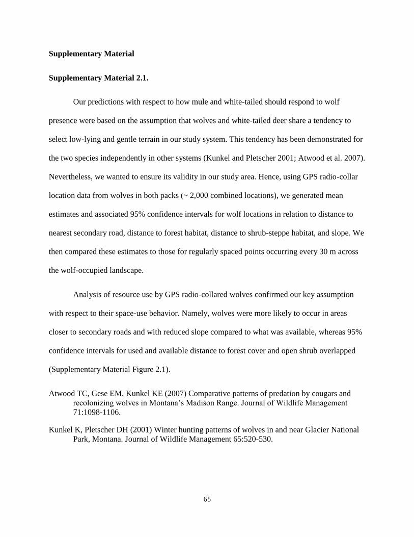
65
Supplementary Material
Supplementary Material 2.1.
Our predictions with respect to how mule and white-tailed should respond to wolf
presence were based on the assumption that wolves and white-tailed deer share a tendency to
select low-lying and gentle terrain in our study system. This tendency has been demonstrated for
the two species independently in other systems (Kunkel and Pletscher 2001; Atwood et al. 2007).
Nevertheless, we wanted to ensure its validity in our study area. Hence, using GPS radio-collar
location data from wolves in both packs (~ 2,000 combined locations), we generated mean
estimates and associated 95% confidence intervals for wolf locations in relation to distance to
nearest secondary road, distance to forest habitat, distance to shrub-steppe habitat, and slope. We
then compared these estimates to those for regularly spaced points occurring every 30 m across
the wolf-occupied landscape.
Analysis of resource use by GPS radio-collared wolves confirmed our key assumption
with respect to their space-use behavior. Namely, wolves were more likely to occur in areas
closer to secondary roads and with reduced slope compared to what was available, whereas 95%
confidence intervals for used and available distance to forest cover and open shrub overlapped
(Supplementary Material Figure 2.1).
Atwood TC, Gese EM, Kunkel KE (2007) Comparative patterns of predation by cougars and
recolonizing wolves in Montana’s Madison Range. Journal of Wildlife Management
71:1098-1106.
Kunkel K, Pletscher DH (2001) Winter hunting patterns of wolves in and near Glacier National
Park, Montana. Journal of Wildlife Management 65:520-530.
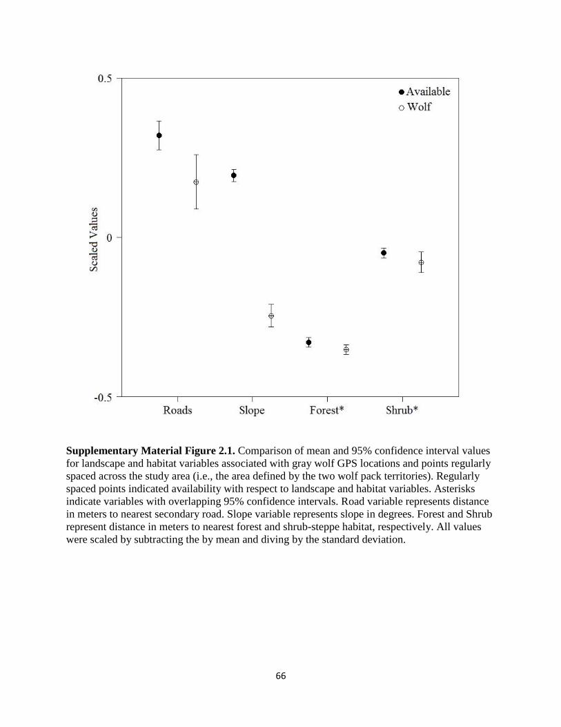
66
Supplementary Material Figure 2.1. Comparison of mean and 95% confidence interval values
for landscape and habitat variables associated with gray wolf GPS locations and points regularly
spaced across the study area (i.e., the area defined by the two wolf pack territories). Regularly
spaced points indicated availability with respect to landscape and habitat variables. Asterisks
indicate variables with overlapping 95% confidence intervals. Road variable represents distance
in meters to nearest secondary road. Slope variable represents slope in degrees. Forest and Shrub
represent distance in meters to nearest forest and shrub-steppe habitat, respectively. All values
were scaled by subtracting the by mean and diving by the standard deviation.
67
Supplementary Material 2.2.
We wanted to verify that deer of both species in wolf-present and wolf-absent areas had
access to the same range of habitat and landscape variables. Accordingly, we compared mean
values and associated 95% confidence intervals between the wolf-present and wolf-absent sites
for all habitat and landscape variables used in the RSFs based on measures from the regularly
spaced points occurring every 30 m (minimum pixel size of spatial data used in analyses) within
the study area.
The wolf-present and wolf-absent study areas were similar with respect to the habitat and
landscape variables used in the analyses of deer space use (distance to roads, distance to forest,
distance to open shrub, and slope; Supplementary Material 2.2).
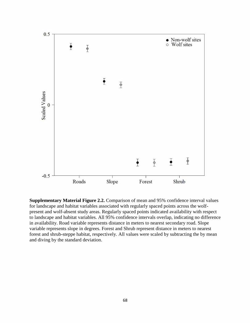
68
Supplementary Material Figure 2.2. Comparison of mean and 95% confidence interval values
for landscape and habitat variables associated with regularly spaced points across the wolf-
present and wolf-absent study areas. Regularly spaced points indicated availability with respect
to landscape and habitat variables. All 95% confidence intervals overlap, indicating no difference
in availability. Road variable represents distance in meters to nearest secondary road. Slope
variable represents slope in degrees. Forest and Shrub represent distance in meters to nearest
forest and shrub-steppe habitat, respectively. All values were scaled by subtracting the by mean
and diving by the standard deviation.
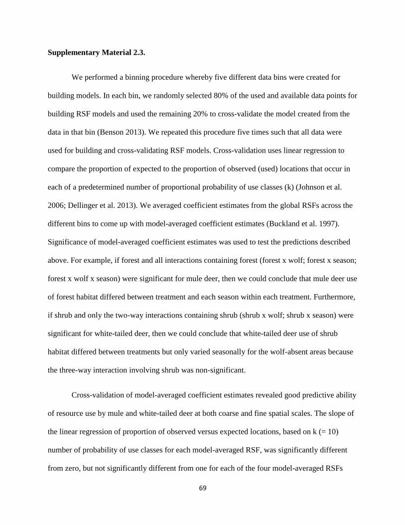
69
Supplementary Material 2.3.
We performed a binning procedure whereby five different data bins were created for
building models. In each bin, we randomly selected 80% of the used and available data points for
building RSF models and used the remaining 20% to cross-validate the model created from the
data in that bin (Benson 2013). We repeated this procedure five times such that all data were
used for building and cross-validating RSF models. Cross-validation uses linear regression to
compare the proportion of expected to the proportion of observed (used) locations that occur in
each of a predetermined number of proportional probability of use classes (k) (Johnson et al.
2006; Dellinger et al. 2013). We averaged coefficient estimates from the global RSFs across the
different bins to come up with model-averaged coefficient estimates (Buckland et al. 1997).
Significance of model-averaged coefficient estimates was used to test the predictions described
above. For example, if forest and all interactions containing forest (forest x wolf; forest x season;
forest x wolf x season) were significant for mule deer, then we could conclude that mule deer use
of forest habitat differed between treatment and each season within each treatment. Furthermore,
if shrub and only the two-way interactions containing shrub (shrub x wolf; shrub x season) were
significant for white-tailed deer, then we could conclude that white-tailed deer use of shrub
habitat differed between treatments but only varied seasonally for the wolf-absent areas because
the three-way interaction involving shrub was non-significant.
Cross-validation of model-averaged coefficient estimates revealed good predictive ability
of resource use by mule and white-tailed deer at both coarse and fine spatial scales. The slope of
the linear regression of proportion of observed versus expected locations, based on k (= 10)
number of probability of use classes for each model-averaged RSF, was significantly different
from zero, but not significantly different from one for each of the four model-averaged RSFs

70
(Supplementary Material Figure 2.3). By implication, the model-averaged coefficient estimates
for each RSF were proportional to the probability of habitat use by both deer species, and both
deer species did not use resources in proportion to availability but rather demonstrated habitat
selection Furthermore, the y-intercept of the linear regression was not significantly different
from zero for each of the four model-averaged RSFs (Supplementary Material Figure 2.3), again
indicating that the model-averaged RSFs were proportional to the probability of habitat use by
both deer species and at each spatial scale. Agreement between the proportions of observed and
expected locations within each probability of use class was high, with all Spearman rank
correlation coefficient values ≥ 0.95 (p < 0.01), demonstrating that each model-averaged RSF
was able to predict habitat use for the respective deer species and spatial scale for individual deer
other than those used to build the RSFs.
Benson JF (2013) Improving rigour and efficiency of use-availability habitat selection analyses
with systematic estimation of availability. Methods in Ecology and Evolution 4:244-251.
Buckland ST, Burnham KP, Augustin NH (1997) Model selection: an integral part of inference.
Biometrics 53:603-618.
Dellinger JA, Proctor C, Steury TD, Kelly MJ, Vaughan MR (2013) Habitat selection of a large
carnivore, the red wolf, in a human-altered landscape. Biological Conservation 157:324-
330.
Johnson CJ, Nielsen SE, Merrill EH, McDonald TL, Boyce MS (2006) Resource selection
functions based on use-availability data: theoretical motivation and evaluation methods.
Journal of Wildlife Management 70:347-357.
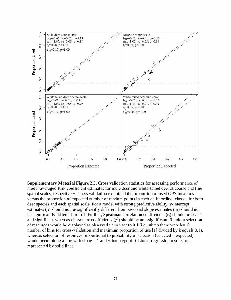
71
Supplementary Material Figure 2.3. Cross validation statistics for assessing performance of
model-averaged RSF coefficient estimates for mule deer and white-tailed deer at coarse and fine
spatial scales, respectively. Cross validation examined the proportion of used GPS locations
versus the proportion of expected number of random points in each of 10 ordinal classes for both
deer species and each spatial scale. For a model with strong predictive ability, y-intercept
estimates (b) should not be significantly different from zero and slope estimates (m) should not
be significantly different from 1. Further, Spearman correlation coefficients (rs) should be near 1
and significant whereas chi-square coefficients (χ2) should be non-significant. Random selection
of resources would be displayed as observed values set to 0.1 (i.e., given there were k=10
number of bins for cross-validation and maximum proportion of use [1] divided by k equals 0.1),
whereas selection of resources proportional to probability of selection (selected = expected)
would occur along a line with slope = 1 and y-intercept of 0. Linear regression results are
represented by solid lines.
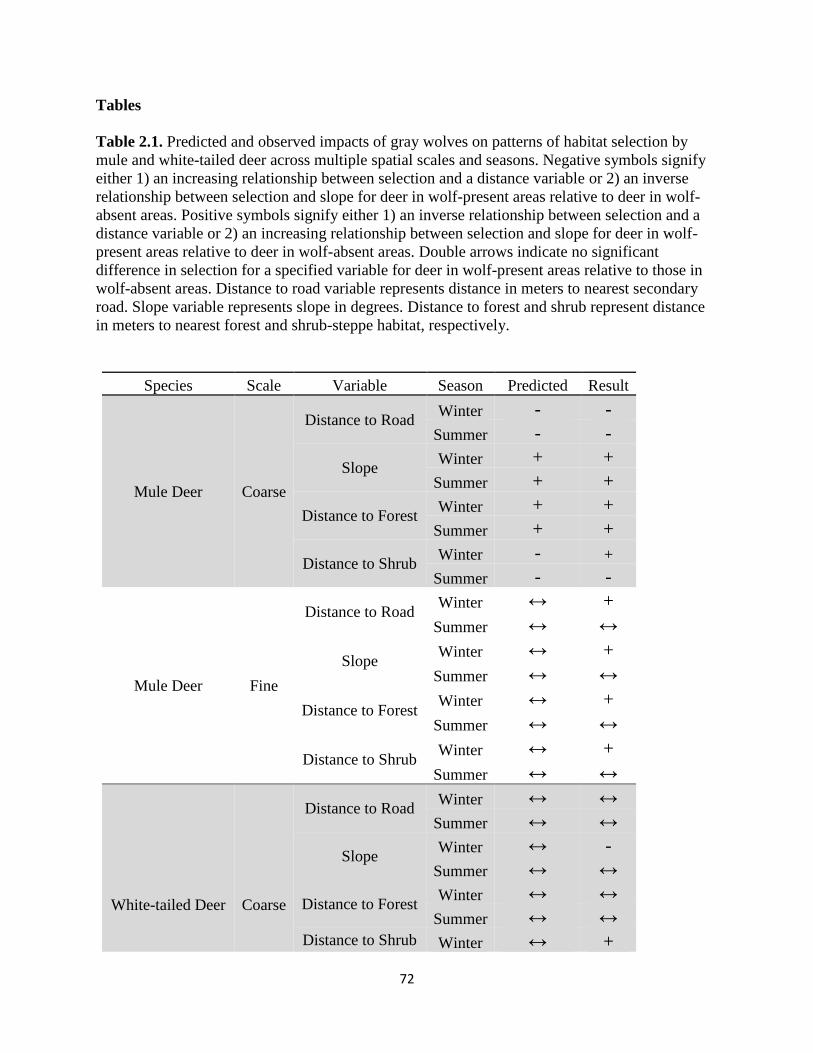
72
Tables
Table 2.1. Predicted and observed impacts of gray wolves on patterns of habitat selection by
mule and white-tailed deer across multiple spatial scales and seasons. Negative symbols signify
either 1) an increasing relationship between selection and a distance variable or 2) an inverse
relationship between selection and slope for deer in wolf-present areas relative to deer in wolf-
absent areas. Positive symbols signify either 1) an inverse relationship between selection and a
distance variable or 2) an increasing relationship between selection and slope for deer in wolf-
present areas relative to deer in wolf-absent areas. Double arrows indicate no significant
difference in selection for a specified variable for deer in wolf-present areas relative to those in
wolf-absent areas. Distance to road variable represents distance in meters to nearest secondary
road. Slope variable represents slope in degrees. Distance to forest and shrub represent distance
in meters to nearest forest and shrub-steppe habitat, respectively.
Species Scale Variable Season Predicted Result
Mule Deer Coarse
Distance to Road Winter - -
Summer - -
Slope Winter + +
Summer + +
Distance to Forest Winter + +
Summer + +
Distance to Shrub Winter - +
Summer - -
Mule Deer Fine
Distance to Road Winter ↔ +
Summer ↔ ↔
Slope Winter ↔ +
Summer ↔ ↔
Distance to Forest Winter ↔ +
Summer ↔ ↔
Distance to Shrub Winter ↔ +
Summer ↔ ↔
White-tailed Deer
Coarse
Distance to Road Winter ↔ ↔
Summer ↔ ↔
Slope Winter ↔ -
Summer ↔ ↔
Distance to Forest Winter ↔ ↔
Summer ↔ ↔
Distance to Shrub Winter ↔ +
73
Summer ↔ ↔
White-tailed Deer Fine
Distance to Road Winter + +
Summer + +
Slope Winter - -
Summer - -
Distance to Forest Winter - -
Summer - -
Distance to Shrub Winter + +
Summer + +
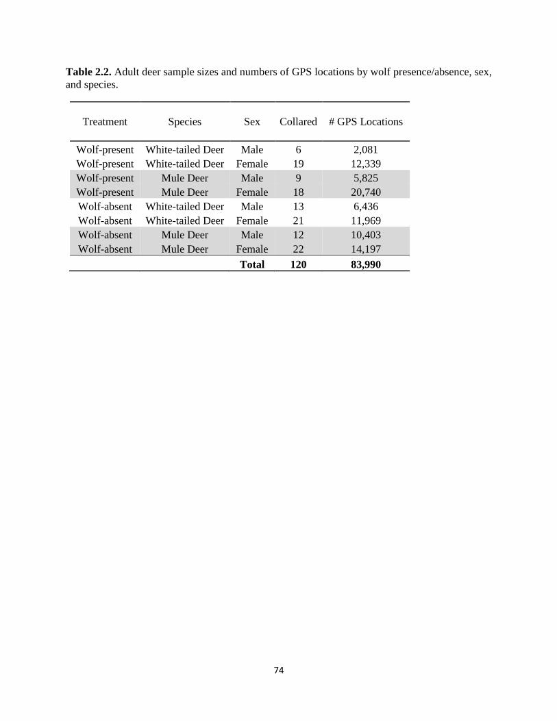
74
Table 2.2. Adult deer sample sizes and numbers of GPS locations by wolf presence/absence, sex,
and species.
Treatment Species Sex Collared # GPS Locations
Wolf-present White-tailed Deer Male 6 2,081
Wolf-present White-tailed Deer Female 19 12,339
Wolf-present Mule Deer Male 9 5,825
Wolf-present Mule Deer Female 18 20,740
Wolf-absent White-tailed Deer Male 13 6,436
Wolf-absent White-tailed Deer Female 21 11,969
Wolf-absent Mule Deer Male 12 10,403
Wolf-absent Mule Deer Female 22 14,197
Total 120 83,990
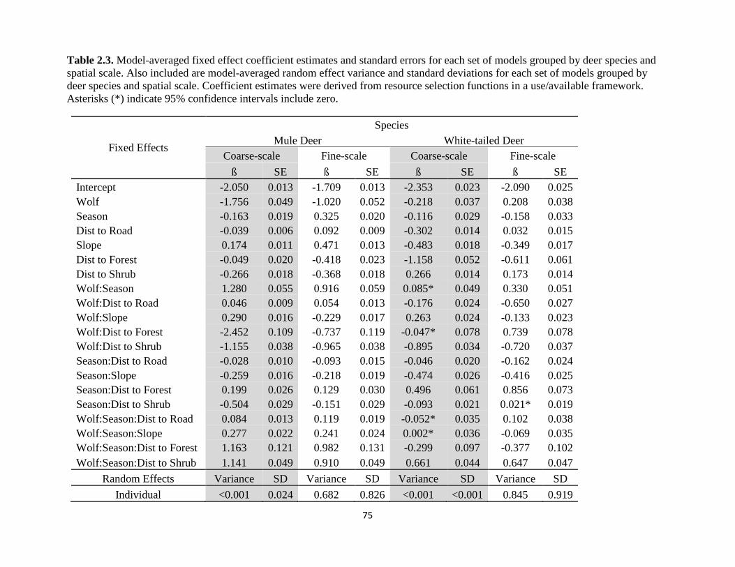
75
Table 2.3. Model-averaged fixed effect coefficient estimates and standard errors for each set of models grouped by deer species and
spatial scale. Also included are model-averaged random effect variance and standard deviations for each set of models grouped by
deer species and spatial scale. Coefficient estimates were derived from resource selection functions in a use/available framework.
Asterisks (*) indicate 95% confidence intervals include zero.
Fixed Effects
Species
Mule Deer White-tailed Deer
Coarse-scale Fine-scale Coarse-scale Fine-scale
ß SE ß SE ß SE ß SE
Intercept -2.050 0.013 -1.709 0.013 -2.353 0.023 -2.090 0.025
Wolf -1.756 0.049 -1.020 0.052 -0.218 0.037 0.208 0.038
Season -0.163 0.019 0.325 0.020 -0.116 0.029 -0.158 0.033
Dist to Road -0.039 0.006 0.092 0.009 -0.302 0.014 0.032 0.015
Slope 0.174 0.011 0.471 0.013 -0.483 0.018 -0.349 0.017
Dist to Forest -0.049 0.020 -0.418 0.023 -1.158 0.052 -0.611 0.061
Dist to Shrub -0.266 0.018 -0.368 0.018 0.266 0.014 0.173 0.014
Wolf:Season 1.280 0.055 0.916 0.059 0.085* 0.049 0.330 0.051
Wolf:Dist to Road 0.046 0.009 0.054 0.013 -0.176 0.024 -0.650 0.027
Wolf:Slope 0.290 0.016 -0.229 0.017 0.263 0.024 -0.133 0.023
Wolf:Dist to Forest -2.452 0.109 -0.737 0.119 -0.047* 0.078 0.739 0.078
Wolf:Dist to Shrub -1.155 0.038 -0.965 0.038 -0.895 0.034 -0.720 0.037
Season:Dist to Road -0.028 0.010 -0.093 0.015 -0.046 0.020 -0.162 0.024
Season:Slope -0.259 0.016 -0.218 0.019 -0.474 0.026 -0.416 0.025
Season:Dist to Forest 0.199 0.026 0.129 0.030 0.496 0.061 0.856 0.073
Season:Dist to Shrub -0.504 0.029 -0.151 0.029 -0.093 0.021 0.021* 0.019
Wolf:Season:Dist to Road 0.084 0.013 0.119 0.019 -0.052* 0.035 0.102 0.038
Wolf:Season:Slope 0.277 0.022 0.241 0.024 0.002* 0.036 -0.069 0.035
Wolf:Season:Dist to Forest 1.163 0.121 0.982 0.131 -0.299 0.097 -0.377 0.102
Wolf:Season:Dist to Shrub 1.141 0.049 0.910 0.049 0.661 0.044 0.647 0.047
Random Effects Variance SD Variance SD Variance SD Variance SD
Individual <0.001 0.024 0.682 0.826 <0.001 <0.001 0.845 0.919
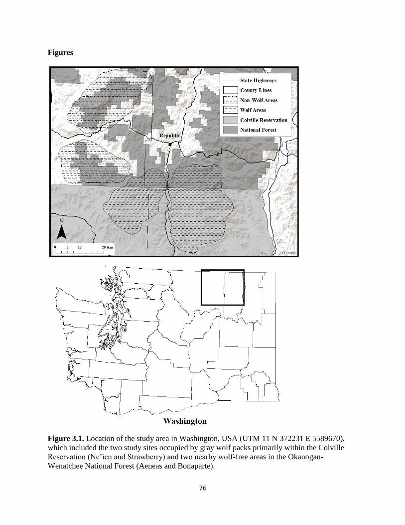
76
Figures
Figure 3.1. Location of the study area in Washington, USA (UTM 11 N 372231 E 5589670),
which included the two study sites occupied by gray wolf packs primarily within the Colville
Reservation (Nc’icn and Strawberry) and two nearby wolf-free areas in the Okanogan-
Wenatchee National Forest (Aeneas and Bonaparte).
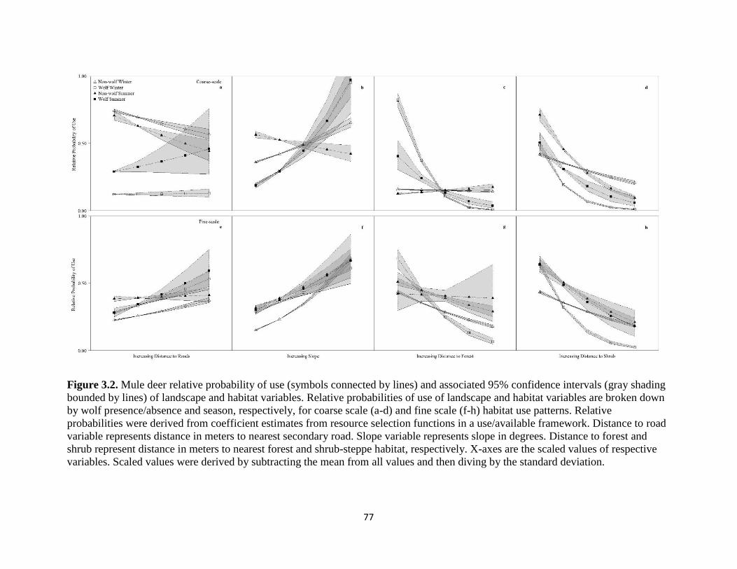
77
Figure 3.2. Mule deer relative probability of use (symbols connected by lines) and associated 95% confidence intervals (gray shading
bounded by lines) of landscape and habitat variables. Relative probabilities of use of landscape and habitat variables are broken down
by wolf presence/absence and season, respectively, for coarse scale (a-d) and fine scale (f-h) habitat use patterns. Relative
probabilities were derived from coefficient estimates from resource selection functions in a use/available framework. Distance to road
variable represents distance in meters to nearest secondary road. Slope variable represents slope in degrees. Distance to forest and
shrub represent distance in meters to nearest forest and shrub-steppe habitat, respectively. X-axes are the scaled values of respective
variables. Scaled values were derived by subtracting the mean from all values and then diving by the standard deviation.

78
Figure 3.3. White-tailed deer relative probability of use (symbols connected by lines) and associated 95% confidence intervals (gray
shading bounded by lines) of landscape and habitat variables. Relative probabilities of use of landscape and habitat variables are
broken down by wolf presence/absence and season, respectively, for coarse scale (a-d) and fine scale (f-h) habitat use patterns.
Relative probabilities were derived from coefficient estimates from resource selection functions in a use/available framework.
Distance to road variable represents distance in meters to nearest secondary road. Slope variable represents slope in degrees. Distance
to forest and shrub represent distance in meters to nearest forest and shrub-steppe habitat, respectively. X-axes are the scaled values of
respective variables. Scaled values were derived by subtracting the mean from all values and then diving by the standard deviation.
79
Chapter 3: Do recolonizing gray wolves impact resource partitioning among sympatric
prey species?
*Pending submission
Abstract: There is increasing recognition of the role predators can play in shaping patterns of
prey resource use. Yet, our understanding of the impacts of predation risk on resource overlap
between co-occurring prey species remains limited, despite the long-appreciated potential for
these impacts to influence patterns of competition and biodiversity. Here, we took advantage of
ongoing gray wolf (Canis lupus) recolonization in northeastern Washington, USA, to contrast
patterns of resource partitioning between sympatric mule deer (Odocoileus hemionus) and white-
tailed deer (O. virginianus) at sites with and without resident wolf packs. Mule and white-tailed
deer have different modes of escaping canid predation (stotting and running, respectively) whose
disparate efficacy on flat terrain appears to contribute to species-specific shifts in resource use in
response to wolf predation risk. Thus, under the hypothesis that wolf exposure influences their
resource overlap, we predicted that features of the landscape relating divergently to the
probability of escaping wolves for the two deer species (e.g., slope, proximity to roads) would be
partitioned to the greatest degree. Given that resource partitioning can manifest at multiple
spatial scales, our analysis employed complimentary approaches to explore partitioning between
the prey species as a function of wolf presence at coarse and fine scales. Redundancy analysis
based on 61 mule deer and 59 white-tailed deer outfitted with GPS radio-collars from 2013-2016
revealed that wolf presence corresponded with the greatest reductions in coarse-scale overlap
along gradients of slope, distance to water, distance to secondary roads, and distance to forest
cover during both summer and winter. Moreover, the ways in which resources were partitioned
at this scale were largely consistent with the two prey species seeking to promote their chances
80
of escape. Latent selection difference models revealed greater fine-scale partitioning of forest
cover in wolf versus non-wolf areas during both seasons, and the manner in which this resource
was partitioned was consistent with species-specific escape facilitation. Thus, our findings
support the idea that wolf predation risk mediates resource partitioning between sympatric deer
species and, insofar as coarse-scale partitioning of slope was especially strong in the wolf-
impacted areas, suggest that escape behavior may play an important role in shaping how
predators alter patterns of resource overlap among their prey. Yet, the magnitudes and directions
of difference in resource overlap between the wolf-affected and wolf-free areas depended on the
resource, season, and scale. By implication, our understanding of the relationship between
predation risk and prey resource partitioning will benefit from a framework that accounts for
these sources of context-dependency.
Introduction
Predators have the potential to promote biodiversity by altering competition among co-
occurring species at lower trophic levels (Paine 1966; Hall et al. 1970; Caswell 1978; Holt 1984;
Sivy et al. 2017). Paine (1966) highlighted the capacity of predators to mediate competition
between sympatric prey species under field conditions. Namely, by experimentally manipulating
the presence of the top predator, the ochre starfish (Pisaster ochraceus), in an intertidal
invertebrate community, he showed that predator removal reduced prey species diversity by
releasing competitively dominant California mussels (Mytilus californianus). Beyond this
pioneering work, however, most field studies of predator effects on interspecific interactions
among sympatric prey species have focused on apparent competition, whereby one relatively
abundant prey species facilitates increased predation on a less common prey species by
supporting increased abundance and distribution of a shared predator (Robinson et al. 2002;
81
DeCesare et al. 2010; Johnson et al. 2013; Wittmer et al. 2013). Accordingly, there remains need
for studies examining how predators shape other types of competitive interactions between co-
occurring prey species under field conditions.
Owing to the challenge of measuring competition directly, most studies seeking to
examine competition instead use resource overlap as a proxy (Colwell and Futuyama 1971;
Pianka 1974; Abrams 1980; Jenkins and Wright 1988). In a classic study, MacArthur (1958)
inferred that five congeneric warbler species are able to coexist despite the potential for strong
interspecific competition by dividing up shared resources. Similarly, Pianka (1974) used indices
of resource overlap to draw inferences about how competition between lizard species was
mediated by environmental variability. More recently, Smith et al. (2018) demonstrated how
human activity mediated competition between co-occurring coyotes (Canis latrans), bobcats
(Lynx rufus), and gray foxes (Urocyon cinereoargenteus) by comparing habitat use and dietary
overlap along a gradient of human activity. Accordingly, we examined patterns of resource
overlap between co-occurring mule deer (Odocoileus hemionus) and white-tailed deer (O.
virginianus) in Washington, USA, to understand how their competitive relationship might be
influenced by recolonizing gray wolves (Canis lupus).
Interactions between gray wolves and their prey in temperate regions of North America
and Europe are well explored (e.g., Mech and Peterson 2003; Ripple and Beschta 2012; Garrott
et al. 2013; Fleming et al. 2017; Winnie and Creel 2017). Only a few studies, however, have
examined their effects on competition between co-occurring prey. In Yellowstone National Park,
for example, direct predation by wolves significantly reduced the abundance and altered the
behavior of elk (Cervus elaphus; Fortin et al. 2005; Evans et al. 2006), resulting in a decrease in
forage overlap between elk and bison (Bison bison) that subsequently appears to have allowed
82
bison numbers to increase (Ripple et al. 2011). Wolf predation risk was also shown to alter
spatial distribution and foraging behavior of elk (Creel et al. 2005; Hernandez and Laundre
2005) and foraging behavior of bison (Laundre et al. 2001), resulting in decreased overlap in
resource use (i.e., food and space) between the two ungulate prey species. In this system,
however, the ability of gray wolves to mediate overlap in resource use between elk and bison
hinges on elk predation (Hernandez et al. 2005) because bison are primarily killed by wolves
when elk are scarce or absent (Smith et al. 2000) and generally only react to wolf predation risk
when under immediate threat (Carbyn and Trottier 1987). By contrast, few studies to date have
examined the capacity of gray wolves to mediate competitive interactions between sympatric
prey species whose susceptibility to predation is more equivalent (e.g., species with more similar
body size and defensive armament).
Previous research shows that mule and white-tailed deer can exhibit considerable forage
and spatial overlap where they co-occur (Kramer 1973; Whittaker and Lindzey 2004; Brunjes et
al. 2006). However, mule deer tend to select for more open terrain at higher elevations whereas
white-tailed deer are more strongly associated with lower elevation habitats that offer greater
concealment (Brunjes et al. 2006). Thus, co-occurrence of the two species is thought to be
promoted by a mosaic of open and dense cover (Brunjes et al. 2006). In regions where
population sizes of the two deer species are asymmetrical, the more abundant species typically
occurs in areas primarily utilized by the other (Whittaker and Lindzey 2004). Under these
circumstances, it is possible that the more abundant species might out compete the other because
of exploitation of shared resources (Kramer 1973) and, further, that wolves could mediate this
process by modifying the extent of prey resource partitioning. To date, however, the impact of
83
wolves on the competitive relationship between mule deer and white-tailed deer has not been
addressed.
Gray wolves began naturally recolonizing Washington state, USA, from northern Idaho
and southern British Columbia, Canada, in 2008. There are currently more than 20 confirmed
packs that are distributed heterogeneously across eastern Washington (Washington Department
of Fish and Wildlife et al. 2017). This patchy wolf distribution enables natural experiments that
contrast prey traits in proximal areas with and without resident packs. Taking advantage of this
opportunity, we quantified patterns of resource overlap between adult mule deer and white-tailed
deer in areas with and without established wolf packs. Mule deer and white-tailed deer have
different escape gaits – stotting (bounding) and running, respectively – whose efficacy is
believed to be promoted by divergent sets of landscape characteristics (Lingle 2002). Namely,
stotting by mule deer is thought to best facilitate predator evasion in areas featuring obstacles
and broken, uneven terrain (Geist 1981), whereas running is believed to allow white-tailed deer
to flee most effectively from predators in areas with gentle terrain that facilitate unobstructed
movement (Kunkel and Pletscher 2001; Kittle et al. 2008). Accordingly, in a previous analysis
we found that mule and white-tailed deer in our study system appear to use space differently in
response to the presence of wolves (Chapter 2). Specifically, relative to conspecifics in wolf-free
areas, mule deer increased their use of two landscape features - steep slopes and areas removed
from roads – that would be expected to enhance the effectiveness of (or reduce the costs
associated with employing) stotting as a means of escape. By contrast, white-tailed deer at risk
from wolves selected gentler slopes and areas more proximal to roads, both of which would be
expected to facilitate fleeing. Given the putative link between these contrasting space use
patterns and gray wolf predation risk, we hypothesized that the presence of wolves might

84
mediate patterns of resource overlap between sympatric mule and white-tailed deer populations,
with landscape features relating divergently to the probability of escaping wolves for the two
prey species being partitioned to the greatest degree. Under this hypothesis, we predicted that
increases in partitioning between mule and white-tailed deer in wolf-occupied versus wolf-free
areas would be most pronounced along gradients of slope and proximity to roads, with mule deer
at risk from wolves shifting away from gentle terrain and roads and the opposite pattern
characterizing white-tailed deer.
Materials and Methods
Study Area
This study took place from 2013-2016 in Okanogan and Ferry Counties of eastern
Washington and included portions of the Okanogan-Wenatchee and Colville National Forests
and the Colville Indian Reservation (See Fig. 1 from Chapter 1). We divided the study area into
four sites, two occupied by gray wolf packs and two that had yet to be colonized, as described in
Chapters 1 and 2. Patterns of habitat composition, human activity, and plant and wildlife species
assemblages within the study area are described in detail in Chapters 1 and 2 and were similar
across the four sites.
Data Collection
We monitored gray wolf activity in all four sites within the study area as described in
Chapters 1 and 2. Briefly, we regularly surveyed roads and game trails for sign, deployed remote
cameras in grid fashion across the landscape (16 cameras per site), and took advantage of
positional data from GPS radio-collars deployed within known wolf packs by the Colville Indian
Reservation Fish and Wildlife Department. None of these monitoring methods revealed any gray
85
wolf pack activity in either wolf-absent site during the course of the study, though we did detect
lone wolves intermittently on our remote game cameras (n = 5 individual detections) that likely
represented dispersing individuals.
To determine coarse- and fine-scale resource partitioning between mule and white-tailed
deer, we captured individuals using a combination of aerial net gunning and baited clover traps
(Haulton et al. 2001) and then outfitted them with GPS radio-collars as described in Chapters 1
and 2. All GPS data were stratified into temporal bins for winter (October-March; i.e., months
with snow cover) and summer (April-September) and spatial bins representing areas where wolf
packs were present versus absent. All animal captures and collar deployments were conducted
under University of Washington Institutional Animal Care and Use Committee (IACUC)
protocol number 4226-01 and wildlife collection permits from the Washington Department of
Fish and Wildlife and the Colville Tribes Fish and Wildlife Department.
Analyses
We estimated mule deer and white-tailed deer partitioning of a number of covariates
serving as potential resources based on previous work (Whittaker and Lindzey 2004; Brunjes et
al. 2006) and matching those we used in Chapter 2. These covariates included elevation
(measured in meters, m), slope (measured in degrees), aspect, distance to nearest secondary road
(m), distance to water (m), and distance to habitat type (m; forest and shrub steppe). Spatial data
on the covariates were obtained from pertinent online data warehouses as described in Chapter 2.
We originally compiled all resource data at a 30 x 30 m resolution (finest resolution possible in a
GIS). We assessed habitat type, secondary roads, and water using a Euclidean Distance Analysis
(EDA) framework (Benson 2013). We estimated the straight-line distance from each pixel (at 30
86
x 30 m resolution) to the nearest secondary road, year-round water source, forest cover, or shrub
steppe habitat. We then standardized these EDA distance values, as well as elevation and slope,
by subtracting each value by the mean and then dividing by the standard deviation to render
coefficient estimates derived from these variables easier to interpret (Benson 2013). We did not
standardize aspect because this covariate ranged from 0 to ≤1.
We anticipated that wolves might mediate patterns of resource overlap between the deer
species at multiple spatial scales based on the results presented in Chapter 2. Thus, we first
examined resource overlap between mule deer and white-tailed deer in wolf and non-wolf areas
at a coarse spatial scale (i.e., 1 km2 cells; the scale of home range establishment; Peters et al.
2013). We examined large-scale overlap as a function of a suite of resource covariates by
analyzing mule deer and white-tailed deer GPS locations across the study area using the
ordination method of redundancy analysis (RDA; Bowman et al. 2010; Peters et al. 2013).
Examination of coarse-scale resource overlap corresponds to measuring inter-specific overlap
between habitat use patterns at the second order scale described by Johnson (1980). Given that
we subsetted the GPS data according to season (summer/winter) and wolf presence/absence,
there were four separate RDA analyses. We classified winter as October-March (i.e., months
with snow cover) and summer as April-September. In RDA, the ordination axes for the species
matrices are constrained linear combinations of the independent variable matrices that result in
the best linear combination of resource covariates that maximize resource partitioning between
the species (ter Braak 1995). Thus, in our case RDA revealed where the two deer species
occurred along gradients of the resource covariates under investigation and attempted to define a
niche space for each within the study area. The RDA analysis resulted in two ordination axes.
The first represented resource covariates that explained separation between species whereas the
87
second represented resource covariates that explained association between species (Bowman et
al. 2010; Peters et al. 2013). Negative coefficient estimates on either ordination axis for any
subset were interpreted such that increasing values of those resource covariates were associated
with mule deer. Conversely, positive coefficient estimates on either ordination axis for any
subset were interpreted such that increasing values of those resource covariates were associated
with white-tailed deer (Peters et al. 2013). Thus, within each treatment subset the deer species
with the smallest difference between their own species score and the coefficient estimates for any
particular resource covariate (Table 1) primarily utilized that resource compared to the other deer
species (Peters et al. 2013). A resource covariate derived using EDA was interpreted such that an
increasing value actually meant getting farther from the resource of interest (e.g., higher values
for distance to secondary road mean increasing distance to secondary road; Benson 2013).
Therefore, the deer species with the largest difference between their own species score and an
EDA-derived coefficient estimate for a resource covariate was positioning itself closer to the
resource.
We conducted RDA analyses by overlaying a 1 x 1 km sampling grid onto our study
region and determining presence and number of GPS locations of each deer species in each grid
cell for each season and wolf treatment. We excluded null values resulting from grid cells that
did not contain any GPS locations. Because all resource covariates were continuous, we
averaged values for each resource variable within each grid cell. We used Monte Carlo
permutation tests to assess the significance of each deer species being constrained to a linear
combination of the resource covariates (999 permutations, α = 0.05; ter Braak 1995). Because
RDA species matrices are constrained to be linear combinations of independent variable
matrices, we evaluated the degree to which the constrained variance accounted for all the
88
variance between the two deer species and the resource covariates. We report the coefficient
estimate of each resource covariate as it relates to each deer species and the scores for each
species (Bowman et al. 2010; Peters et al. 2013). Lastly, we calculated the graphical distance
between scores for each deer species and coefficient estimates for each resource covariate,
respectively. We compared these differences between the two deer species to determine whether
they increased or decreased along coarse-scale resource gradients as a function of wolf treatment
within each season (Ramette 2007). For example, an increased difference between each species’
score and distance to forest cover, respectively, in wolf versus non-wolf areas would indicate
increased partitioning of forest cover in the wolf-occupied areas.
We next examined fine-scale resource partitioning between mule deer and white-tailed
deer in wolf and non-wolf areas by using logistic regression (Hosmer and Lemeshow 2000) to
estimate coefficients for latent selection difference (LSD) functions (Mueller et al. 2004; Latham
et al. 2011; Peters et al. 2013). Examination of fine-scale resource partitioning corresponds to
exploring differences in resource overlap at the third-order scale (i.e., use of resources within the
home range) described by Johnson (1980). For this analysis, we coded mule deer used locations
as 1 and white-tailed deer used locations as 0 (Latham et al. 2011) and intersected locations with
spatial data at the 30 x 30 m resolution. As with RDA analyses, we subsetted the data according
to season (summer/winter) and wolf presence/absence to examine impacts of wolf presence on
seasonal resource partitioning. Given that we subsetted the data, there were four separate LSD
functions modeled. We estimated degree of resource partitioning using the β coefficients from
LSD functions. Negative coefficients indicated greater use by white-tailed deer compared to
mule deer and positive coefficients indicated greater resource use by mule deer compared to
white-tailed deer (Latham et al. 2011). For example, a positive coefficient estimate for elevation
89
would indicate greater use of higher elevations by mule deer relative to white-tailed deer.
However, EDA derived coefficients had to be interpreted differently. Namely, a negative
coefficient estimate for distance to secondary road would indicate greater use of areas farther
from secondary roads by white-tailed deer relative to mule deer. Once coefficient estimates were
derived, the resulting value of 𝑒𝛽 for each positive coefficient estimate indicated that with every
unit increase in the value of or distance to a given resource, the amount of partitioning of that
resource between mule deer and white-tailed deer increased or decreased, respectively, by x%.
Conversely, negative coefficient estimates were transformed using -[1-𝑒𝛽] x 100 and quantified
the extent of partitioning of resources between white-tailed deer and mule deer (Czetwertynski
2007). We plotted these χ% relative resource partitioning differences to visually assess seasonal
differences in fine-scale resource partitioning between mule deer and white-tailed deer in wolf
and non-wolf areas. A potential outcome supporting our main prediction would be an increase in
percent resource partitioning of sloped terrain or areas close to roads between mule deer and
white-tailed deer in wolf-occupied areas relative to non-wolf areas.
Using 80% of the GPS locations, we built global LSD functions for each of the four data
subsets according to season and wolf treatment using all individual resource covariates
mentioned above at a 30 x 30m resolution (i.e., the finest resolution possible). We screened all
resource covariates for collinearity using the Pearson’s correlation coefficient threshold of r >
0.5, retaining the collinear variable with the higher log-likelihood and lowest p-value as
determined using univariate logistic regression analysis. We then used Akaike’s Information
Criterion corrected for small sample size (AICc) to determine the most parsimonious LSD
models (Anderson and Burnham 2002). Following model building, we used the remaining 20%
of the GPS locations to test the predictive capabilities of LSD models for mule deer and white-
90
tailed deer resource overlap (Boyce et al. 2002; Johnson et al. 2006; Benson 2013; Dellinger et
al. 2013). To complete this step, we translated coefficient estimates of our most parsimonious
LSD models predicting mule deer and white-tailed deer fine-scale resource overlap into spatial
predictive maps (Hirzel and Le Lay 2008) using Raster Calculator in ArcMap (ESRI, Redlands,
California). We used the raster layers of resource covariates mentioned above to aid in deriving
the spatial predictive maps of resource partitioning. The resulting maps contained pixels with
values ranging from 0-1, which represented predicted resource partitioning by mule deer or
white-tailed deer. In our predictive maps, values closer to 1 indicated increased resource
partitioning with mule deer primarily utilizing the resources at the given area and, conversely,
values closer to 0 indicated increased resource partitioning with white-tailed deer primarily
utilizing the resources at the given area. Thus, extreme values (i.e., near 1 or 0) indicated areas of
little resource overlap between the two deer species whereas intermediate values (e.g., 0.3-0.7)
indicated areas of increased resource overlap between the two deer species (Peters et al. 2013).
We then classified the predicted probabilities of mule and white-tailed deer use across the study
area into 10 equal-sized bins (0-0.1, 0.1-0.2, etc.; Boyce et al. 2002), and used the test data to
assess Spearman’s correlation between expected and observed number of GPS locations of each
deer species in each bin (Johnson et al. 2006). Lastly, we counted the frequency of GPS locations
by each species in each bin. This served as cross-validation of the most parsimonious LSD
models (Peters et al. 2013). Predictive ability of the most parsimonious models should result in:
1) high correlation between expected and observed numbers of GPS locations of each deer
species in each bin; 2) a high proportion of mule deer GPS locations in the bins containing
higher values (i.e., 0.8-1); and 3) a high proportion of white-tailed deer GPS locations in the bins
containing lower values (i.e., 0.1-0.3).
91
We used Program R version 3.1.2 (R Core Team 2017) for all statistical analyses, and
ArcView GIS version 10.2 Geographic Information System (GIS; ESRI, Redlands, California)
and Geospatial Modeling Environment version 0.7.4.0 (Beyer 2015) for spatial analyses. In all
analyses, we considered P ≤ 0.05 to be statistically significant.
Results
Over the course of three years, we collared 120 adult deer (n = 61 mule deer, n = 59
white-tailed deer). We collected an average of 700 locations (± 562 sd) per radio-collared
individual and monitored individuals for an average of 433 days (± 275 sd).
Using RDA analysis, we found that the suite of resources covariates significantly defined
coarse-scale resource overlap between mule deer and white-tailed deer. The relationship between
the resource overlap of mule deer and white-tailed deer and the resources covariates was
significant for all season by wolf treatment subsets (wolf winter: F8, 1031 = 12.22, p < 0.01; non-
wolf winter: F7, 1217 = 7.84, p < 0.01; wolf summer: F8, 1203 = 9.59, p < 0.01; non-wolf summer:
F7,1424 = 14.38, p < 0.01). The first RDA ordination axis primarily explained the constrained
variance of the linear species-resource covariate relationship for each subset of data (Table 1),
whereas the second RDA ordination axis explained relatively little. Thus, the resource covariates
we used better explained resource partitioning between the two species rather than their
association (Peters et al. 2013).
For each season by wolf treatment subset, RDA analyses revealed coarse-scale resource
partitioning between mule deer and white-tailed deer. In each instance, relative species scores for
first ordination axes were largely opposite one another, indicating resource partitioning between
the two prey species. Coefficient estimates for elevation, slope, proximity to water, and roads
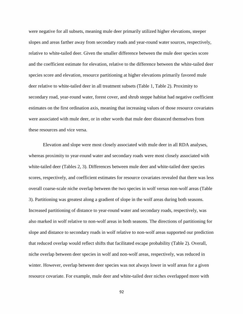
92
were negative for all subsets, meaning mule deer primarily utilized higher elevations, steeper
slopes and areas farther away from secondary roads and year-round water sources, respectively,
relative to white-tailed deer. Given the smaller difference between the mule deer species score
and the coefficient estimate for elevation, relative to the difference between the white-tailed deer
species score and elevation, resource partitioning at higher elevations primarily favored mule
deer relative to white-tailed deer in all treatment subsets (Table 1, Table 2). Proximity to
secondary road, year-round water, forest cover, and shrub steppe habitat had negative coefficient
estimates on the first ordination axis, meaning that increasing values of those resource covariates
were associated with mule deer, or in other words that mule deer distanced themselves from
these resources and vice versa.
Elevation and slope were most closely associated with mule deer in all RDA analyses,
whereas proximity to year-round water and secondary roads were most closely associated with
white-tailed deer (Tables 2, 3). Differences between mule deer and white-tailed deer species
scores, respectively, and coefficient estimates for resource covariates revealed that there was less
overall coarse-scale niche overlap between the two species in wolf versus non-wolf areas (Table
3). Partitioning was greatest along a gradient of slope in the wolf areas during both seasons.
Increased partitioning of distance to year-round water and secondary roads, respectively, was
also marked in wolf relative to non-wolf areas in both seasons. The directions of partitioning for
slope and distance to secondary roads in wolf relative to non-wolf areas supported our prediction
that reduced overlap would reflect shifts that facilitated escape probability (Table 2). Overall,
niche overlap between deer species in wolf and non-wolf areas, respectively, was reduced in
winter. However, overlap between deer species was not always lower in wolf areas for a given
resource covariate. For example, mule deer and white-tailed deer niches overlapped more with

93
respect to aspect and proximity to shrub steppe in non-wolf versus wolf areas in both seasons
(Table 2).
Using LSD analysis, we found that the suite of resource covariates significantly
predicted fine-scale resource partitioning between mule deer and white-tailed deer. All resource
covariates were included in the most parsimonious models for wolf sites in winter and non-wolf
sites in summer (Table 3). Distance to secondary roads was not in the most parsimonious model
for non-wolf sites in winter and aspect was not in the most parsimonious model for wolf sites in
summer. Resource partitioning of higher elevations, steeper slopes, and areas closer to year-
round water and shrub steppe habitat, respectively, favored mule deer relative to white-tailed
deer in all subsets. Resource partitioning between the deer species varied with wolf treatment
and season. In non-wolf areas, resource partitioning of more exposed aspects (i.e., south-
southwest) favored mule deer and partitioning of more sheltered aspects (i.e., north-northeast)
favored white-tailed deer, respectively, in both seasons. This relationship was opposite in wolf
areas in winter such that resource partitioning of exposed aspects favored white-tailed deer
whereas partitioning of sheltered aspects favored mule deer. Furthermore, in non-wolf areas
resource partitioning of areas farther from forest cover favored mule deer in both seasons. Again,
that relationship was opposite in wolf areas in both seasons, with mule deer selecting for areas
close to forest cover relative to white-tailed deer, which shifted into the open. Fine-scale
partitioning of slope revealed that mule deer utilized steeper slopes relative to white-tailed deer
in all treatments and seasons. However, increased partitioning of slope in wolf relative to non-
wolf areas only occurred in summer and the difference in overlap during this season was modest
(i.e., it increased from 3.50% to 3.95% as a function of wolf presence; Fig. 1, Table 4). Lastly,
fine-scale partitioning of secondary roads revealed that mule deer utilized areas farther from

94
secondary roads relative to white-tailed deer in all treatments and seasons except non-wolf areas
in summer. Increased partitioning of secondary roads in wolf relative to non-wolf areas only
occurred in winter and the difference in overlap during this season was modest (i.e., it increased
from 1.02% to 3.31% as a function of wolf presence; Fig. 1, Table 4). Thus, fine-scale directions
and magnitudes of partitioning of slope and distance to secondary roads in wolf relative to non-
wolf areas did not support our prediction of escape facilitation (Table 4). In winter, overall fine-
scale resource partitioning between mule deer and white-tailed deer was greater in wolf versus
non-wolf sites. In summer, overall fine-scale resource portioning between mule deer and white-
tailed deer was more similar between wolf treatments but the amount of partitioning of
individual resources between the two deer species varied between wolf treatments (Fig. 1, Table
4).
The most-parsimonious LSD models for each data subset had good predictive ability. All
of the most-parsimonious LSD models had high Spearman correlation coefficients (wolf winter:
average rs = 0.97, p < 0.01; non-wolf winter: average rs = 0.99, p < 0.01; wolf summer: average rs
= 0.99, p < 0.01; non-wolf summer: average rs = 0.98, p < 0.01). By implication, withheld GPS
location data agreed with expected number of GPS locations in each bin derived from the most
parsimonious LSD models. Furthermore, high proportions of mule deer and white-tailed deer
GPS locations from the test data were contained within the bins containing higher and lower
probability of use values, respectively (Fig. 2), demonstrating a high ability to predict resource
partitioning between the two deer species in wolf present/absent areas and season.
Discussion
95
Taking advantage of the return of grey wolves to a multi-prey landscape in the American
west, we found support for the hypothesis that wolf predation risk mediates patterns of resource
overlap between sympatric ungulate prey. Specifically, during winter, coarse-scale resource
partitioning between mule deer and white-tailed deer increased in areas with gray wolves relative
to wolf-free sites for all resources except aspect and distance to shrub steppe, and fine-scale
resource partitioning increased in the presence of wolves for all resources save slope.
Accordingly, our results suggest that gray wolves may structure competitive interactions among
prey in large-mammal communities. Moreover, the direction of partitioning of some resources in
the wolf-impacted areas, notably slope and roads at the coarse spatial scale of analysis, putatively
facilitated the respective escape modes of the two deer species, suggesting that prey escape
behavior could play an important role in shaping how predators alter patterns of resource overlap
among their prey. Yet, in summer, both coarse- and fine-scale resource partitioning between the
prey species did not change markedly in response to wolf presence, and the magnitude and
direction of differences in resource partitioning between the wolf-occupied and wolf-free areas
varied with spatial scale. Indeed, partitioning of some resources such as shrub-steppe habitat and
aspect was unchanged or even decreased in the presence of wolves at the coarse-scale. By
implication, the relationship between predation risk and prey resource partitioning is resource-
specific and hinges on spatiotemporal context.
A number of studies have demonstrated the ability of bottom-up and abiotic processes
like seral stage and fire to mediate resource overlap between ungulates (Brunjes et al. 2006;
Sittler et al. 2015). Along with research in the Greater Yellowstone Ecosystem (e.g., Laundre et
al. 2001; Creel et al. 2005; Hernandez and Laundre 2005), our findings suggest that top-down
processes like predation risk from wolves can also mediate resource overlap between co-
96
occurring ungulate prey. To the extent that patterns of resource overlap reflect competition, then,
wolves may help to structure large mammal communities by influencing competition among
their ungulate prey species. Notably, the wolves in our study system existed at densities that are
comparable to other human-modified ecosystems and lower than those more typical of protected
areas (Jimenez and Becker 2016). Nevertheless, we detected an apparent relationship between
wolf predation risk and resource overlap between mule and white-tailed deer, hinting at the
potential for even stronger wolf impacts on prey competition where their numbers and
distribution are not constrained by humans (Kuijper et al. 2015). We acknowledge, however, that
our results are correlative, preventing us from controlling for other possible environmental
drivers of resource partitioning between the prey species. Accordingly, there remains need for
studies capable of simultaneously examining bottom-up and top-down forcing of prey resource
partitioning and, by extension, competition.
Previous research in eastern Washington revealed that white-tailed deer exhibit higher
survival and population growth rates than sympatric mule deer (Robinson et al. 2002). Moreover,
in a case of apparent competition, increasing spatial overlap between mule and white-tailed deer
with expansion of the latter species has apparently led to elevated cougar (Puma concolor)
predation on mule deer (Robinson et al. 2002). Thus, high resource overlap between the two
species could negatively affect mule deer populations in Washington. Insofar as wolves drive
resource partitioning between mule and white-tailed deer, then, continued expansion of this top
predator in Washington could not only alter competition between these two deer species but also
reduce cougar predation on mule deer stemming from apparent competition. It is also possible,
however, that mule deer shifts away from low-lying areas hunted by wolves could place them at
greater risk of predation by cougars, which tend to target prey in areas offering stalking cover
97
and rugged terrain (Atwood et al. 2009). Thus, there is need for studies aimed at discriminating
between these two possible scenarios.
We predicted that mule and white-tailed deer at risk from wolves would be especially
likely to increase their partitioning of landscape features with divergent effects on their modes of
escape. For example, we expected mule and white-tailed deer in the presence of wolves to
increase their partitioning of slope because steeper slopes inhibit wolf travel and white-tailed
deer sprinting but facilitate mule deer stotting (Lingle 2002; Mech and Peterson 2003; Oakleaf et
a. 2006). In support of this expectation, mule deer and white-tailed deer increased their
partitioning of slope in wolf versus non-wolf areas except during winter at the fine spatial scale.
When faced with wolf predation risk, mule deer utilized steeper slopes and white-tailed deer
utilized more gentle terrain (Table 2, Table 4). Similarly, we expected that mule and white-tailed
deer at risk from wolves would increase their partitioning of roaded areas because roads tend to
be established in gentle, low-lying areas that facilitate sprinting by white-tailed deer but reduce
the effectiveness of stotting (Kunkel and Pletscher 2001; Lingle 2002). Again supporting this
expectation, mule deer and white-tailed deer increased their partitioning of roaded areas in wolf
versus non-wolf areas save during summer at the fine spatial scale. Specifically, mule deer
utilized areas farther from roads whereas white-tailed deer utilized areas closer to roads in wolf
relative to non-wolf areas (Tables 2, 4). In general, therefore, we suggest that a framework
incorporating the relationship between prey escape behavior and landscape features should aid in
predicting how patterns of prey resource partitioning are likely to be shaped by spatiotemporal
variation in predation risk.
In a previous analysis (Chapter 2), we found that only mule deer altered their use of
forest cover when at risk from wolves relative to conspecifics in wolf-free areas. Here, therefore,
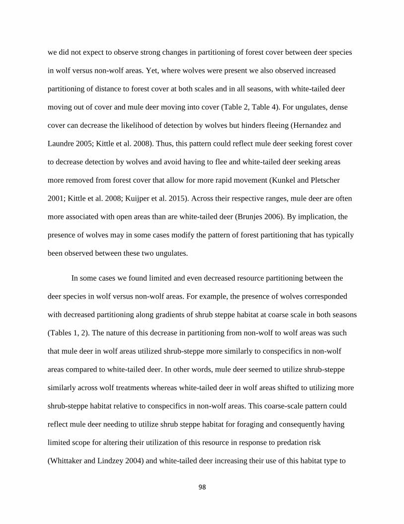
98
we did not expect to observe strong changes in partitioning of forest cover between deer species
in wolf versus non-wolf areas. Yet, where wolves were present we also observed increased
partitioning of distance to forest cover at both scales and in all seasons, with white-tailed deer
moving out of cover and mule deer moving into cover (Table 2, Table 4). For ungulates, dense
cover can decrease the likelihood of detection by wolves but hinders fleeing (Hernandez and
Laundre 2005; Kittle et al. 2008). Thus, this pattern could reflect mule deer seeking forest cover
to decrease detection by wolves and avoid having to flee and white-tailed deer seeking areas
more removed from forest cover that allow for more rapid movement (Kunkel and Pletscher
2001; Kittle et al. 2008; Kuijper et al. 2015). Across their respective ranges, mule deer are often
more associated with open areas than are white-tailed deer (Brunjes 2006). By implication, the
presence of wolves may in some cases modify the pattern of forest partitioning that has typically
been observed between these two ungulates.
In some cases we found limited and even decreased resource partitioning between the
deer species in wolf versus non-wolf areas. For example, the presence of wolves corresponded
with decreased partitioning along gradients of shrub steppe habitat at coarse scale in both seasons
(Tables 1, 2). The nature of this decrease in partitioning from non-wolf to wolf areas was such
that mule deer in wolf areas utilized shrub-steppe more similarly to conspecifics in non-wolf
areas compared to white-tailed deer. In other words, mule deer seemed to utilize shrub-steppe
similarly across wolf treatments whereas white-tailed deer in wolf areas shifted to utilizing more
shrub-steppe habitat relative to conspecifics in non-wolf areas. This coarse-scale pattern could
reflect mule deer needing to utilize shrub steppe habitat for foraging and consequently having
limited scope for altering their utilization of this resource in response to predation risk
(Whittaker and Lindzey 2004) and white-tailed deer increasing their use of this habitat type to
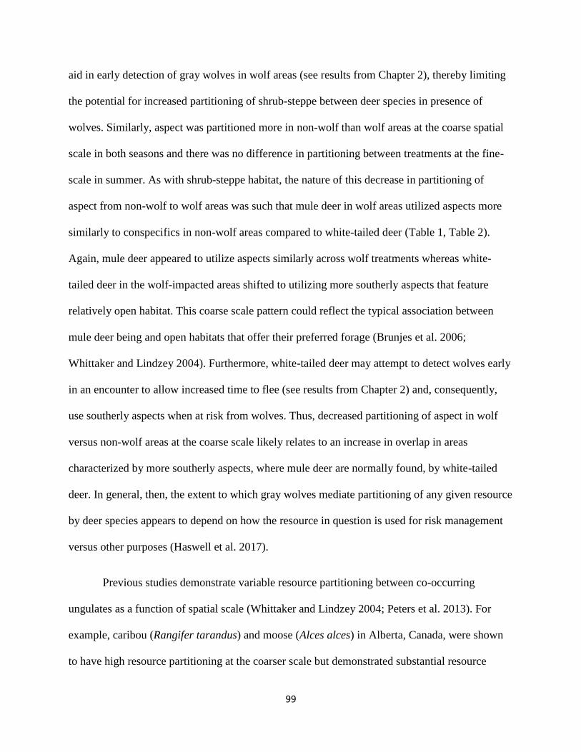
99
aid in early detection of gray wolves in wolf areas (see results from Chapter 2), thereby limiting
the potential for increased partitioning of shrub-steppe between deer species in presence of
wolves. Similarly, aspect was partitioned more in non-wolf than wolf areas at the coarse spatial
scale in both seasons and there was no difference in partitioning between treatments at the fine-
scale in summer. As with shrub-steppe habitat, the nature of this decrease in partitioning of
aspect from non-wolf to wolf areas was such that mule deer in wolf areas utilized aspects more
similarly to conspecifics in non-wolf areas compared to white-tailed deer (Table 1, Table 2).
Again, mule deer appeared to utilize aspects similarly across wolf treatments whereas white-
tailed deer in the wolf-impacted areas shifted to utilizing more southerly aspects that feature
relatively open habitat. This coarse scale pattern could reflect the typical association between
mule deer being and open habitats that offer their preferred forage (Brunjes et al. 2006;
Whittaker and Lindzey 2004). Furthermore, white-tailed deer may attempt to detect wolves early
in an encounter to allow increased time to flee (see results from Chapter 2) and, consequently,
use southerly aspects when at risk from wolves. Thus, decreased partitioning of aspect in wolf
versus non-wolf areas at the coarse scale likely relates to an increase in overlap in areas
characterized by more southerly aspects, where mule deer are normally found, by white-tailed
deer. In general, then, the extent to which gray wolves mediate partitioning of any given resource
by deer species appears to depend on how the resource in question is used for risk management
versus other purposes (Haswell et al. 2017).
Previous studies demonstrate variable resource partitioning between co-occurring
ungulates as a function of spatial scale (Whittaker and Lindzey 2004; Peters et al. 2013). For
example, caribou (Rangifer tarandus) and moose (Alces alces) in Alberta, Canada, were shown
to have high resource partitioning at the coarser scale but demonstrated substantial resource

100
overlap at the finer scale because of similar utilization of open early seral stage habitat (Peters et
al. 2013). We also found that partitioning of particular resources by mule and white-tailed deer in
wolf versus non-wolf sites was not consistent across the two scales of analysis. For example, at
the coarse-scale, increased resource partitioning between the deer species in the wolf areas
occurred along gradients of slope, distance to year-round water, secondary roads, and forest
cover in all seasons. However, at the finer scale, increased resource partitioning in wolf versus
non-wolf areas only occurred for distance to forest cover in all seasons (Fig. 1, Table 4). This
disparity could owe to the different scales at which the two deer species make resource use and
anti-predator decisions. Namely, mule deer have been shown to prioritize foraging needs over
predation risk (Pierce et al. 2004). Like other ungulates, mule deer feeding decisions are
normally made at fine spatial scales because energetic benefit and palatability vary from plant to
plant (Whittaker and Lindzey 2004). Furthermore, in our study system, mule deer appear to
manage predation risk from wolves at the coarse scale (Chapter 2). Conversely, white-tailed deer
are thought to prioritize predation risk over foraging needs (Whittaker and Lindzey 2004) and, in
our system, appear to account for predation risk by wolves at the fine scale (Chapter 2). Thus, we
might expect wolf-mediated partitioning patterns at the coarse scale to reflect mule deer anti-
predator adjustments and overlap patterns at the finer scale to be more a product of the interplay
between mule deer feeding choices and white-tailed deer risk management. More broadly,
because many sympatric prey species likely prioritize foraging needs differently and respond to
predation risk at differing spatial scales, our findings suggest that studies addressing a single
spatial scale may miss key predator effects on prey resource partitioning. Accordingly, future
research should consider multiple scales simultaneously when investigating impacts of predators
on competitive interactions between multiple co-occurring prey species.
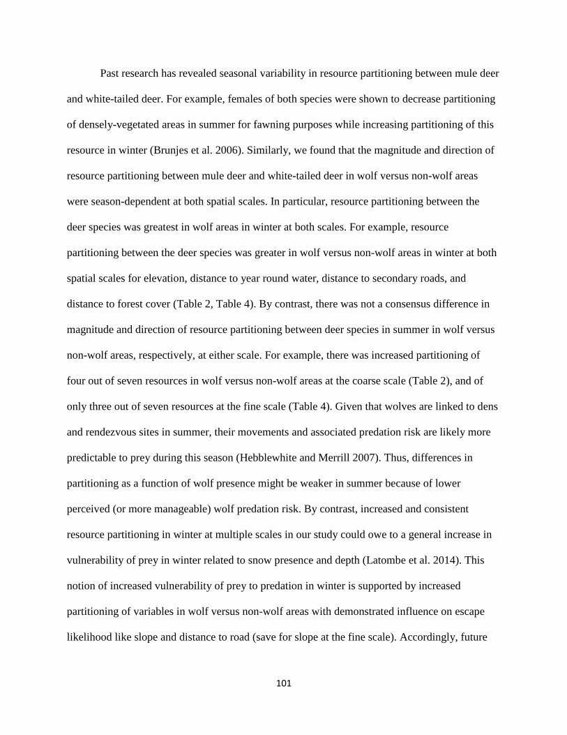
101
Past research has revealed seasonal variability in resource partitioning between mule deer
and white-tailed deer. For example, females of both species were shown to decrease partitioning
of densely-vegetated areas in summer for fawning purposes while increasing partitioning of this
resource in winter (Brunjes et al. 2006). Similarly, we found that the magnitude and direction of
resource partitioning between mule deer and white-tailed deer in wolf versus non-wolf areas
were season-dependent at both spatial scales. In particular, resource partitioning between the
deer species was greatest in wolf areas in winter at both scales. For example, resource
partitioning between the deer species was greater in wolf versus non-wolf areas in winter at both
spatial scales for elevation, distance to year round water, distance to secondary roads, and
distance to forest cover (Table 2, Table 4). By contrast, there was not a consensus difference in
magnitude and direction of resource partitioning between deer species in summer in wolf versus
non-wolf areas, respectively, at either scale. For example, there was increased partitioning of
four out of seven resources in wolf versus non-wolf areas at the coarse scale (Table 2), and of
only three out of seven resources at the fine scale (Table 4). Given that wolves are linked to dens
and rendezvous sites in summer, their movements and associated predation risk are likely more
predictable to prey during this season (Hebblewhite and Merrill 2007). Thus, differences in
partitioning as a function of wolf presence might be weaker in summer because of lower
perceived (or more manageable) wolf predation risk. By contrast, increased and consistent
resource partitioning in winter at multiple scales in our study could owe to a general increase in
vulnerability of prey in winter related to snow presence and depth (Latombe et al. 2014). This
notion of increased vulnerability of prey to predation in winter is supported by increased
partitioning of variables in wolf versus non-wolf areas with demonstrated influence on escape
likelihood like slope and distance to road (save for slope at the fine scale). Accordingly, future
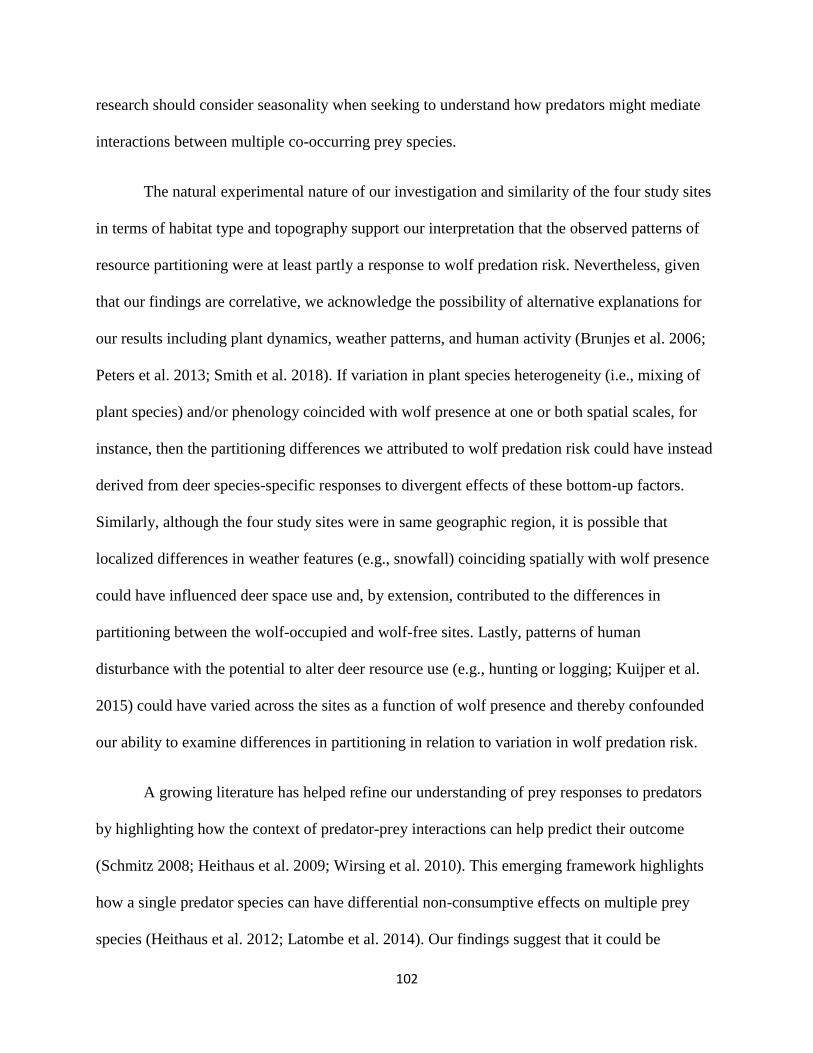
102
research should consider seasonality when seeking to understand how predators might mediate
interactions between multiple co-occurring prey species.
The natural experimental nature of our investigation and similarity of the four study sites
in terms of habitat type and topography support our interpretation that the observed patterns of
resource partitioning were at least partly a response to wolf predation risk. Nevertheless, given
that our findings are correlative, we acknowledge the possibility of alternative explanations for
our results including plant dynamics, weather patterns, and human activity (Brunjes et al. 2006;
Peters et al. 2013; Smith et al. 2018). If variation in plant species heterogeneity (i.e., mixing of
plant species) and/or phenology coincided with wolf presence at one or both spatial scales, for
instance, then the partitioning differences we attributed to wolf predation risk could have instead
derived from deer species-specific responses to divergent effects of these bottom-up factors.
Similarly, although the four study sites were in same geographic region, it is possible that
localized differences in weather features (e.g., snowfall) coinciding spatially with wolf presence
could have influenced deer space use and, by extension, contributed to the differences in
partitioning between the wolf-occupied and wolf-free sites. Lastly, patterns of human
disturbance with the potential to alter deer resource use (e.g., hunting or logging; Kuijper et al.
2015) could have varied across the sites as a function of wolf presence and thereby confounded
our ability to examine differences in partitioning in relation to variation in wolf predation risk.
A growing literature has helped refine our understanding of prey responses to predators
by highlighting how the context of predator-prey interactions can help predict their outcome
(Schmitz 2008; Heithaus et al. 2009; Wirsing et al. 2010). This emerging framework highlights
how a single predator species can have differential non-consumptive effects on multiple prey
species (Heithaus et al. 2012; Latombe et al. 2014). Our findings suggest that it could be
103
extended beyond bilateral predator-prey relationships to include more complex non-consumptive
interactions between prey species responding to a shared predator. For example, resource overlap
between two sympatric prey species with a shared predator is likely to depend on similarity in
their escape behavior, which dictates how prey will position themselves spatially to reduce
predation risk (Laundre et al. 2014). Furthermore, the presence of multiple shared predators with
different hunting modes could influence resource partitioning between sympatric prey species to
the extent that different landscape features facilitate prey escape/capture and predator
success/failure. Accordingly, we encourage further work that explores prey resource partitioning
under predation risk while explicitly accounting for drivers of context dependence including how
specific resources relate to escape behavior, scale, and temporal heterogeneity.

104
Literature Cited
Anderson DR, Burnham KP (2002) Avoiding pitfalls when using information theoretic methods.
Journal of Wildlife Management 66:912-918.
Atwood TC, Gese EM, Kunkel KE (2009) Spatial partitioning of predation risk in a multiple
predator-multiple prey system. Journal of Wildlife Management 73:876-884.
Benson JF (2013) Improving rigour and efficiency of use-availability habitat selection analyses
with systematic estimation of availability. Methods in Ecology and Evolution 4:244-251.
Beyer HL (2015) Geospatial Modelling Environment (Version 0.7.4.0). URL:
http://www.spatialecology.com/gme.
Bowman J, Ray JC, Magoun AJ, Johnson DS, Dawson FN (2010) Roads, logging, and large-
mammal community of an eastern Canadian boreal forest. Canadian Journal of Zoology
88:454–467.
Boyce MS, Vernier PR, Nielsen SE, Schmiegelow FK (2002) Evaluating resource selection
functions. Ecological Modelling 157:281-300.
Brunjes KJ, Ballard WB, Humphrey MH, Harwell F, McIntyre NE, Krausman PR, Wallace MC
(2006) Habitat use by sympatric mule and white-tailed deer in Texas. Journal of Wildlife
Management 70:1351-1359.
Carbyn LN, Trottier T (1987) Responses of bison on their calving grounds to predation by
wolves in Wood Buffalo National Park. Canadian Journal of Zoology 65:2072-2078.
Creel S, Winnie Jr JA, Maxwell B, Hamlin K, Creel M (2005) Elk alter habitat selection as an
antipredator response to wolves. Ecology 86:3387-3397.
Czetwertynski SM (2007) Effects of hunting on the demographics, movement, and habitat
selection of American black bears (Ursus americanus). Ph.D. thesis. Department of
Renewable Resources, University of Alberta, Edmonton.
Dellinger JA, Proctor C, Steury TD, Kelly MJ, Vaughan MR (2013) Habitat selection of a large
carnivore, the red wolf, in a human-altered landscape. Biological Conservation 157:324-
330.
DeCesare NJ, Hebblewhite M, Robinson HS, Musiani M (2010) Endangered, apparently: the role
of apparent competition in endangered species conservation. Animal Conservation
13:353-362.
Evans SB, Mech LD, White PJ, Sargeant GA (2006) Survival of adult female elk in
Yellowstone following wolf restoration. Journal of Wildlife Management 70:1372-1378.
105
Fortin D, Beyer HL, Boyce MS, Smith DW, Duchesne T, Mao JS (2005) Wolves influence elk
movements: behavior shapes a trophic cascade in Yellowstone National Park. Ecology
86:1320-1330.
Garrott RA, White P, Waston FGR (2013) The ecology of large mammals in central
Yellowstone: Sixteen years of integrated field studies. Academic Press, New York.
Geist V (1981) Behavior: adaptive strategies in mule deer. In: Wallmo, O. C., editor. Mule and
black-tailed deer of North America. University of Nebraska Press, Lincoln. Pp. 157–224.
Haswell PM, Kusak J, Hayward MW (2017) Large carnivore impacts are context-dependent.
Food Webs 12:3-13.
Haulton SM, Porter WF, Rudolph BA (2001) Evaluating 4 methods to capture white-tailed deer.
Wildlife Society Bulletin 29:255-264.
Hebblewhite M, Merrill EH (2007) Multiscale wolf predation risk for elk: does migration reduce
risk? Oecologia 152:377-387.
Heithaus MR, Wirsing AJ, Dill LM (2012) The ecological importance of intact top-predator
populations: a synthesis of 15 years of research in a seagrass ecosystem. Marine and
Freshwater Research 63:1039-1050.
Heithaus MR, Wirsing AJ, Burkholder D, Thomson J, Dill LM (2009) Towards a predictive
framework for predator risk effects: the interaction of landscape features and prey escape
tactics. Journal of Animal Ecology 78:556-562.
Hernandez L, Laundre JW (2005) Foraging in the landscape of fear and its implications for
habitat use and diet quality of elk Cervus elaphus and bison Bison bison. Wildlife
Biology 11:215-220.
Hirzel AH, Le Lay G (2008) Habitat suitability modelling and niche theory. Journal of Applied
Ecology 45:1372–1381.
Hosmer DW, Lemeshow S (2000) Applied logistic regression. Wiley Publishing, New York.
Jimenez MD, Becker SA (2016) Northern Rocky Mountain Wolf Recovery Program 2015
Interagency Annual Report. U.S. Fish and Wildlife Service, Ecological Services, 585
Shepard Way, Helena, Montana, 59601.
Johnson CJ, Nielsen SE, Merrill EH, McDonald TL, Boyce MS (2006) Resource selection
functions based on use-availability data: theoretical motivation and evaluation methods.
Journal of Wildlife Management 70:347-357.
Johnson HE, Hebblewhite M, Stephenson TR, German DW, Pierce BM, Bleich VC (2013)
Evaluating apparent competition in limiting the recovery of an endangered ungulate.
Oecologia 171:295-307.
106
Johnson DH (1980) The comparison of usage and availability measurements for evaluating
resource preference. Ecology 61:65-71.
Kittle AM, Fryxell JM, Desy GE, Hamr J (2008) The scale-dependent impact of wolf predation
risk on resource selection by three sympatric ungulates. Oecologia 157:163-175.
Kuijper DPJ, Sahlen E, Elmhagen B, Chamaille-Jammes S, Sand H, Lone K, Cromsigt JPGM
(2016) Paws without claws? Ecological effects of large carnivores in anthropogenic
landscapes. Proceedings of the Royal Society B 283:1625
Kuijper DPJ, Bubnicki JW, Churski M, Mols B, Van Hooft P (2015) Context dependence of risk
effects: wolves and tree logs create patches of fear in an old-growth forest. Behavioral
Ecology 26:1558-1568.
Kunkel K, Pletscher DH (2001) Winter hunting patterns of wolves in and near Glacier National
Park, Montana. Journal of Wildlife Management 65:520-530.
Latham ADM, Latham MC, Boyce MS (2011) Habitat selection and spatial relationships of
black bears (Ursus americanus) with woodland caribou (Rangifer tarandus caribou) in
northeastern Alberta. Canadian Journal of Zoology 89:267-277.
Latombe G, Fortin D, Parrott L (2014) Spatio-temporal dynamics in the response of woodland
caribou and moose to the passage of grey wolf. Journal of Animal Ecology 83:185-198.
Laundre JW, Hernandez L, Altendorf KB (2001) Wolves, elk, and bison: reestablishing the
landscape of fear in Yellowstone National Park, USA. Canadian Journal of Zoology
79:1401-1409.
Laundre JW, Hernandez L, Medina PL, Campanella A, Lopez-Portillo J, Gonzalez-Romero A,
Grajales-Tam K, Burke AM, Gronmeyer P, Browning DM (2014) The landscape of fear:
the missing link to understand top-down and bottom-up controls of prey abundance?
Ecology 95:1141-1152.
Lingle S (2002) Coyote predation and habitat segregation of white-tailed deer and mule deer.
Ecology 83:2037-2048.
Mech LD, Peterson RO (2003) Wolf-prey relations. In Wolves: Behavior, Ecology, and
Conservation. Edited by L.D. Mech and L. Boitani. University of Chicago Press. 131-160
pp.
Mueller C, Herrero S, Gibeau ML (2004) Distribution of subadult grizzly bears in relation to
human development in the Bow River watershed, Alberta. Ursus 15:35-47.
Oakleaf JK, Murray DL, Oakleaf JR, Bangs EE, Mack CM, Smith DW, Fontaine JA, Jimenez
MD, Meier TJ, Niemeyer CC (2006) Habitat selection by recolonizing wolves in the
northern Rocky Mountains of the United States. Journal of Wildlife Management 70:554-
563.

107
Paine RT (1966) Food web complexity and species diversity. The American Naturalist 100:65-
75.
Peters W, Hebblewhite M, DeCesare N, Cagnacci F, Musian M (2013) Resource separation
analysis with moose indicates threats to caribou in human altered landscapes. Ecography
36:487-498.
Pierce BM, Bowyer RT, Bleich VC (2004) Habitat selection by mule deer: forage benefits or risk
of predation? Journal of Wildlife Management 68:533-541.
R Core Team (2017) R: A language and environment for statistical computing. R Foundation for
Statistical Computing, Vienna, Austria. URL: https://www.R-project.org/.
Ramette A (2007) Multivariate analyses in microbial ecology. FEMS Microbiology Ecology
62:142-160.
Ripple WJ, Painter LE, Beschta RL, Gates CC (2011) Wolves, elk, bison, and secondary trophic
cascades in Yellowstone National Park. Open Ecology Journal 3:31-37.
Ripple WJ, Beschta RL (2012) Trophic cascades in Yellowstone: the first 15 years after wolf
reintroduction. Biological Conservation 145:205-213.
Robinson HS, Wielgus RB, Gwilliam JC (2002) Cougar predation and population growth of
sympatric mule deer and white-tailed deer. Canadian Journal of Zoology 80:556-568.
ter Braak C (1995) Chapter 5: ordination. In: Jongman, R. et al. (eds), Data analysis in
community and landscape ecology. Cambridge Univ. Press, pp. 91–173.
Schmitz OJ (2008) Effects of predator hunting mode on grassland ecosystem functioning.
Science 319:952-954.
Smith DW, Mech LD, Meagher M, Clark WE, Jaffe R, Phillips MK, Mack JA (2000) Wolf-
bison interactions in Yellowstone National Park. Journal of Mammalogy 81:1128-1135.
Smith JA (2018) Human activity reduces niche partitioning among three widespread
mesocarnivores. Oikos doi:10.1111/oik.04592.
Washington Department of Fish and Wildlife, Confederated Colville Tribes, Spokane Tribe of
Indians, USDA-APHIS Wildlife Services, and U.S. Fish and Wildlife Service. 2017.
Washington Gray Wolf Conservation and Management 2016 Annual Report. Washington
Department of Fish and Wildlife, Colville, WA, USA.
Whittaker DG, Lindzey FG (2004) Habitat use patterns of sympatric deer species on Rocky
Mountain Arsenal, Colorado. Wildlife Society Bulletin 32:1114-1123.
Winnie J, Creel S (2017) The many effects of carnivores on their prey and their implications for
trophic cascades, and ecosystem structure and function. Food Webs 12:88-94.

108
Wirsing AJ, Cameron KE, Heithaus MR (2010) Spatial responses to predators vary with prey
escape mode. Animal Behavior 79:531-537.
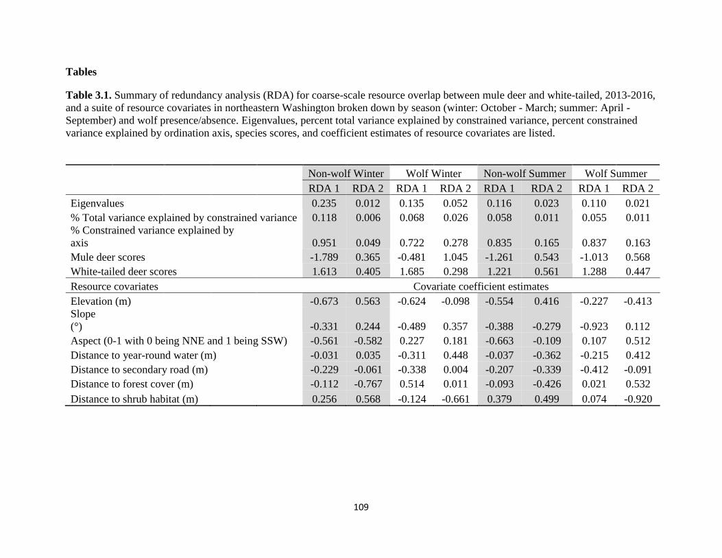
109
Tables
Table 3.1. Summary of redundancy analysis (RDA) for coarse-scale resource overlap between mule deer and white-tailed, 2013-2016,
and a suite of resource covariates in northeastern Washington broken down by season (winter: October - March; summer: April -
September) and wolf presence/absence. Eigenvalues, percent total variance explained by constrained variance, percent constrained
variance explained by ordination axis, species scores, and coefficient estimates of resource covariates are listed.
Non-wolf Winter Wolf Winter Non-wolf Summer Wolf Summer
RDA 1 RDA 2 RDA 1 RDA 2 RDA 1 RDA 2 RDA 1 RDA 2
Eigenvalues 0.235 0.012 0.135 0.052 0.116 0.023 0.110 0.021
% Total variance explained by constrained variance 0.118 0.006 0.068 0.026 0.058 0.011 0.055 0.011
% Constrained variance explained by
axis 0.951 0.049 0.722 0.278 0.835 0.165 0.837 0.163
Mule deer scores -1.789 0.365 -0.481 1.045 -1.261 0.543 -1.013 0.568
White-tailed deer scores 1.613 0.405 1.685 0.298 1.221 0.561 1.288 0.447
Resource covariates Covariate coefficient estimates
Elevation (m) -0.673 0.563 -0.624 -0.098 -0.554 0.416 -0.227 -0.413
Slope
(°) -0.331 0.244 -0.489 0.357 -0.388 -0.279 -0.923 0.112
Aspect (0-1 with 0 being NNE and 1 being SSW) -0.561 -0.582 0.227 0.181 -0.663 -0.109 0.107 0.512
Distance to year-round water (m) -0.031 0.035 -0.311 0.448 -0.037 -0.362 -0.215 0.412
Distance to secondary road (m) -0.229 -0.061 -0.338 0.004 -0.207 -0.339 -0.412 -0.091
Distance to forest cover (m) -0.112 -0.767 0.514 0.011 -0.093 -0.426 0.021 0.532
Distance to shrub habitat (m) 0.256 0.568 -0.124 -0.661 0.379 0.499 0.074 -0.920
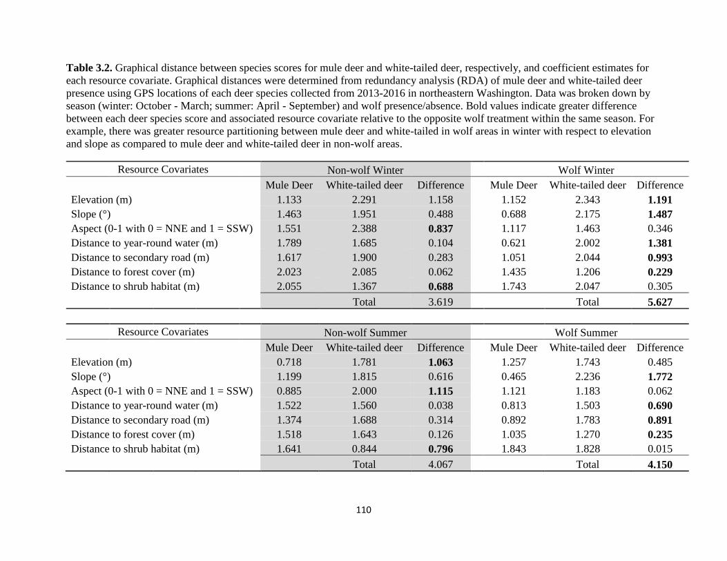
110
Table 3.2. Graphical distance between species scores for mule deer and white-tailed deer, respectively, and coefficient estimates for
each resource covariate. Graphical distances were determined from redundancy analysis (RDA) of mule deer and white-tailed deer
presence using GPS locations of each deer species collected from 2013-2016 in northeastern Washington. Data was broken down by
season (winter: October - March; summer: April - September) and wolf presence/absence. Bold values indicate greater difference
between each deer species score and associated resource covariate relative to the opposite wolf treatment within the same season. For
example, there was greater resource partitioning between mule deer and white-tailed in wolf areas in winter with respect to elevation
and slope as compared to mule deer and white-tailed deer in non-wolf areas.
Resource Covariates Non-wolf Winter Wolf Winter
Mule Deer White-tailed deer Difference Mule Deer White-tailed deer Difference
Elevation (m) 1.133 2.291 1.158 1.152 2.343 1.191
Slope (°) 1.463 1.951 0.488 0.688 2.175 1.487
Aspect (0-1 with 0 = NNE and 1 = SSW) 1.551 2.388 0.837 1.117 1.463 0.346
Distance to year-round water (m) 1.789 1.685 0.104 0.621 2.002 1.381
Distance to secondary road (m) 1.617 1.900 0.283 1.051 2.044 0.993
Distance to forest cover (m) 2.023 2.085 0.062 1.435 1.206 0.229
Distance to shrub habitat (m) 2.055 1.367 0.688 1.743 2.047 0.305
Total 3.619 Total 5.627
Resource Covariates Non-wolf Summer Wolf Summer
Mule Deer White-tailed deer Difference Mule Deer White-tailed deer Difference
Elevation (m) 0.718 1.781 1.063 1.257 1.743 0.485
Slope (°) 1.199 1.815 0.616 0.465 2.236 1.772
Aspect (0-1 with 0 = NNE and 1 = SSW) 0.885 2.000 1.115 1.121 1.183 0.062
Distance to year-round water (m) 1.522 1.560 0.038 0.813 1.503 0.690
Distance to secondary road (m) 1.374 1.688 0.314 0.892 1.783 0.891
Distance to forest cover (m) 1.518 1.643 0.126 1.035 1.270 0.235
Distance to shrub habitat (m) 1.641 0.844 0.796 1.843 1.828 0.015
Total 4.067 Total 4.150
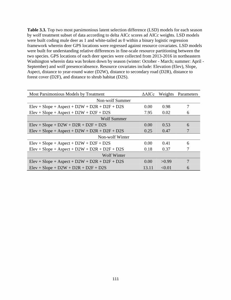
111
Table 3.3. Top two most parsimonious latent selection difference (LSD) models for each season
by wolf treatment subset of data according to delta AICc scores ad AICc weights. LSD models
were built coding mule deer as 1 and white-tailed as 0 within a binary logistic regression
framework wherein deer GPS locations were regressed against resource covariates. LSD models
were built for understanding relative differences in fine-scale resource partitioning between the
two species. GPS locations of each deer species were collected from 2013-2016 in northeastern
Washington wherein data was broken down by season (winter: October - March; summer: April -
September) and wolf presence/absence. Resource covariates include: Elevation (Elev), Slope,
Aspect, distance to year-round water (D2W), distance to secondary road (D2R), distance to
forest cover (D2F), and distance to shrub habitat (D2S).
Most Parsimonious Models by Treatment ΔAICc Weights Parameters
Non-wolf Summer
Elev + Slope + Aspect + D2W + D2R + D2F + D2S 0.00 0.98 7
Elev + Slope + Aspect + D2W + D2F + D2S 7.95 0.02 6
Wolf Summer
Elev + Slope + D2W + D2R + D2F + D2S 0.00 0.53 6
Elev + Slope + Aspect + D2W + D2R + D2F + D2S 0.25 0.47 7
Non-wolf Winter
Elev + Slope + Aspect + D2W + D2F + D2S 0.00 0.41 6
Elev + Slope + Aspect + D2W + D2R + D2F + D2S 0.18 0.37 7
Wolf Winter
Elev + Slope + Aspect + D2W + D2R + D2F + D2S 0.00 >0.99 7
Elev + Slope + D2W + D2R + D2F + D2S 13.11 <0.01 6
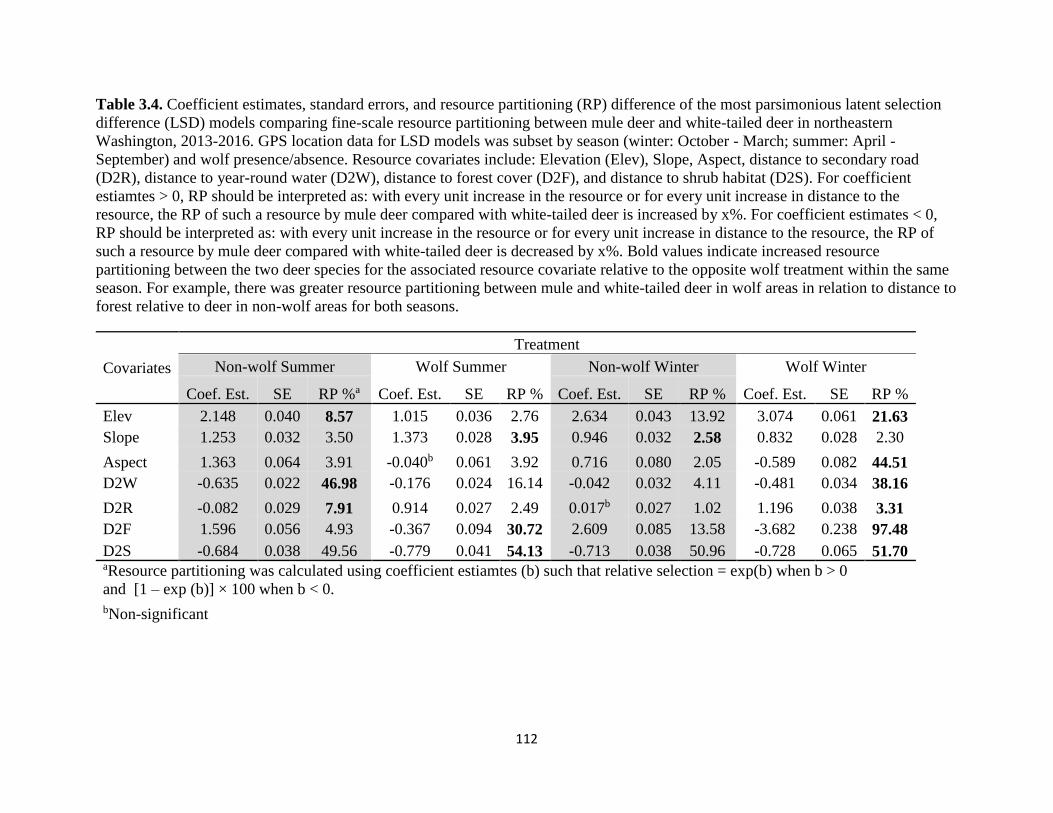
112
Table 3.4. Coefficient estimates, standard errors, and resource partitioning (RP) difference of the most parsimonious latent selection
difference (LSD) models comparing fine-scale resource partitioning between mule deer and white-tailed deer in northeastern
Washington, 2013-2016. GPS location data for LSD models was subset by season (winter: October - March; summer: April -
September) and wolf presence/absence. Resource covariates include: Elevation (Elev), Slope, Aspect, distance to secondary road
(D2R), distance to year-round water (D2W), distance to forest cover (D2F), and distance to shrub habitat (D2S). For coefficient
estiamtes > 0, RP should be interpreted as: with every unit increase in the resource or for every unit increase in distance to the
resource, the RP of such a resource by mule deer compared with white-tailed deer is increased by x%. For coefficient estimates < 0,
RP should be interpreted as: with every unit increase in the resource or for every unit increase in distance to the resource, the RP of
such a resource by mule deer compared with white-tailed deer is decreased by x%. Bold values indicate increased resource
partitioning between the two deer species for the associated resource covariate relative to the opposite wolf treatment within the same
season. For example, there was greater resource partitioning between mule and white-tailed deer in wolf areas in relation to distance to
forest relative to deer in non-wolf areas for both seasons.
Covariates
Treatment
Non-wolf Summer Wolf Summer Non-wolf Winter Wolf Winter
Coef. Est. SE RP %a Coef. Est. SE RP % Coef. Est. SE RP % Coef. Est. SE RP %
Elev 2.148 0.040 8.57 1.015 0.036 2.76 2.634 0.043 13.92 3.074 0.061 21.63
Slope 1.253 0.032 3.50 1.373 0.028 3.95 0.946 0.032 2.58 0.832 0.028 2.30
Aspect 1.363 0.064 3.91 -0.040b 0.061 3.92 0.716 0.080 2.05 -0.589 0.082 44.51
D2W -0.635 0.022 46.98 -0.176 0.024 16.14 -0.042 0.032 4.11 -0.481 0.034 38.16
D2R -0.082 0.029 7.91 0.914 0.027 2.49 0.017b 0.027 1.02 1.196 0.038 3.31
D2F 1.596 0.056 4.93 -0.367 0.094 30.72 2.609 0.085 13.58 -3.682 0.238 97.48
D2S -0.684 0.038 49.56 -0.779 0.041 54.13 -0.713 0.038 50.96 -0.728 0.065 51.70 aResource partitioning was calculated using coefficient estiamtes (b) such that relative selection = exp(b) when b > 0
and [1 – exp (b)] × 100 when b < 0.
bNon-significant
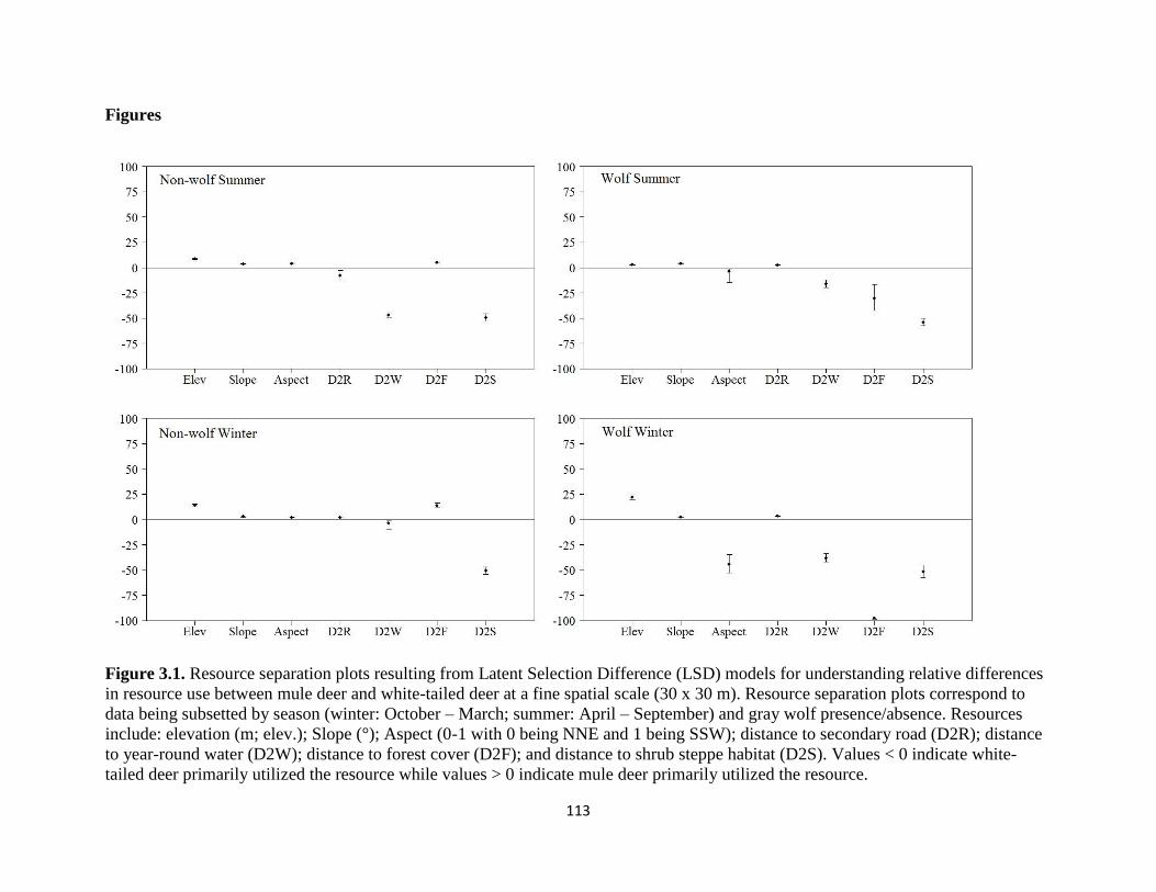
113
Figures
Figure 3.1. Resource separation plots resulting from Latent Selection Difference (LSD) models for understanding relative differences
in resource use between mule deer and white-tailed deer at a fine spatial scale (30 x 30 m). Resource separation plots correspond to
data being subsetted by season (winter: October – March; summer: April – September) and gray wolf presence/absence. Resources
include: elevation (m; elev.); Slope (°); Aspect (0-1 with 0 being NNE and 1 being SSW); distance to secondary road (D2R); distance
to year-round water (D2W); distance to forest cover (D2F); and distance to shrub steppe habitat (D2S). Values < 0 indicate white-
tailed deer primarily utilized the resource while values > 0 indicate mule deer primarily utilized the resource.
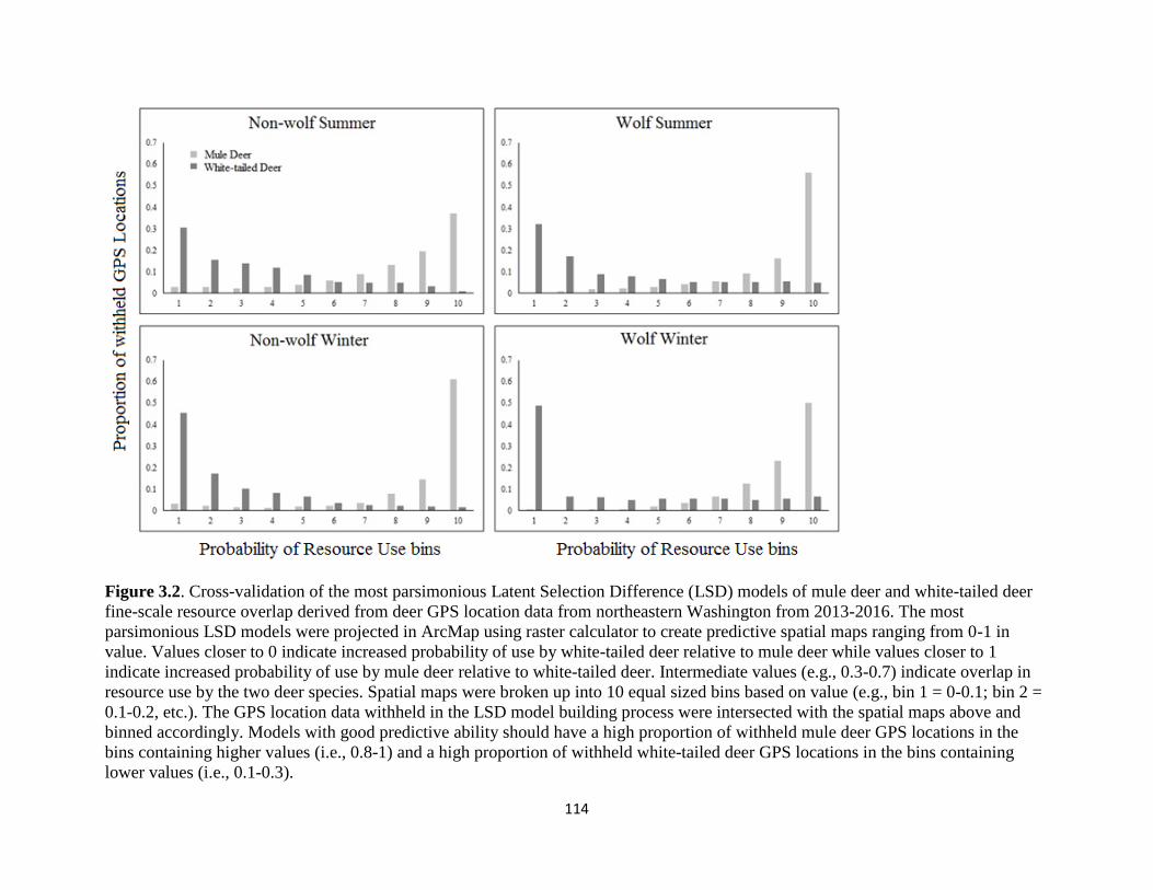
114
Figure 3.2. Cross-validation of the most parsimonious Latent Selection Difference (LSD) models of mule deer and white-tailed deer
fine-scale resource overlap derived from deer GPS location data from northeastern Washington from 2013-2016. The most
parsimonious LSD models were projected in ArcMap using raster calculator to create predictive spatial maps ranging from 0-1 in
value. Values closer to 0 indicate increased probability of use by white-tailed deer relative to mule deer while values closer to 1
indicate increased probability of use by mule deer relative to white-tailed deer. Intermediate values (e.g., 0.3-0.7) indicate overlap in
resource use by the two deer species. Spatial maps were broken up into 10 equal sized bins based on value (e.g., bin 1 = 0-0.1; bin 2 =
0.1-0.2, etc.). The GPS location data withheld in the LSD model building process were intersected with the spatial maps above and
binned accordingly. Models with good predictive ability should have a high proportion of withheld mule deer GPS locations in the
bins containing higher values (i.e., 0.8-1) and a high proportion of withheld white-tailed deer GPS locations in the bins containing
lower values (i.e., 0.1-0.3).