1

Impedance-based Fault Location inTransmission Networks: Theory and Application

Swagata Das,Student Member, IEEE,Surya Santoso,Senior Member, IEEE,Anish Gaikwad,Senior Member, IEEE,and Mahendra Patel,Senior Member, IEEE

Abstract—Several impedance-based fault location algorithmshave been developed in the literature for locating faults in atransmission network. Choosing the best approach for faultlocation from such a wide selection of impedance-based faultlocation algorithms is a challenging task and requires a de-tailed understanding of the working principle of each fault-locating method. Therefore, the objectives of this paper areto present a comprehensive review of impedance-based faultlocation algorithms described in the IEEE C37.114 Standardand to evaluate the performance of each fault-locating algorithm,given an error source. Another objective in this paper is to assesswhat additional information can be gleaned from waveformscaptured by intelligent electronic devices (IEDs) during a fault.Actual fault event data from utility networks is exploited to gainvaluable feedback about the transmission network upstream fromthe IED device, and estimate the value of fault resistance, whichis useful for identifying the root-cause of the fault and validatingthe short-circuit model of the transmission network. Finally, thepaper recommends the following criteria for choosing the mostsuitable fault-locating algorithm: (a) data availability, and (b)fault location application scenario.

Index Terms—Fault location, power system faults, impedance-measurement, intelligent electronic devices (IED), power systemreliability, transmission line measurements.

I. NOMENCLATURE

ρ Earth resistivity (Ωm)ds Current distribution factorβ Phase angle ofds (degrees)e−jβ Non-homogeneity correction factor (degrees)ejδ Synchronization operator (degrees)m Distance to the fault (pu)D Distance of the tap point from terminal G (pu)RF Fault resistance (Ω)IF Current at the fault point F (kA)IT Fault current from terminal T (kA)IJ0 Zero-sequence current in the parallel transmission

line at terminal G (kA)VTap Voltage at the tap point during fault (kV)Zapp Apparent impedance to the fault (Ω)Z0M Zero-sequence mutual coupling (Ω)Z012 Sequence line impedance matrix (Ω)ZLoad Load impedance (Ω)

This work was supported by Electric Power Research Institute (EPRI).S. Das and S. Santoso are with the Department of Electrical & Computer

Engineering, The University of Texas at Austin, Austin, TX 78712 (e-mail:swagata@utexas.edu, ssantoso@mail.utexas.edu).

A. Gaikwad and M. Patel are with EPRI, Knoxville, TN 37932 (e-mail:AGaikwad@epri.com, MPatel@epri.com).

VF1pre Positive-sequence prefault voltage at thefault point F (kV)

VAB , VCA Line-to-line fault voltages between phasesA and B, and phases C and A (kV)

EG, EH Internal source voltages at terminals G andH (kV)

ZG, ZH Source impedances of terminals G and H(Ω)

IG, IH Line currents during fault at terminals Gand H (kA)

VG, VH Line-to-ground voltages recorded during thefault at terminals G and H (kV)

IJ , IK Line currents in the parallel transmissionline at terminals G and H (kA)

IJ2, IK2 Negative-sequence currents in the paralleltransmission line at terminals G and H (kA)

∆VG,∆VH “Pure fault” voltages at terminals G and H(kV)

∆IG,∆IH “Pure fault” currents at terminals G and H(kA)

IApre, IBpre,ICpre

Prefault currents in phases A, B, and C atterminal G (kA)

VG1pre, VH1pre Positive-sequence prefault voltages at termi-nals G and H (kV)

IG1pre, IH1pre Positive-sequence prefault currents at termi-nals G and H (kA)

IG0, IG1, IG2 Sequence components of the fault current atterminal G (kA)

IH0, IH1, IH2 Sequence components of the fault current atterminal H (kA)

IAF , IBF , ICF Fault currents in phases A, B, and C atterminal G (kA)

VAF , VBF , VCF Fault voltages in phases A, B, and C atterminal G (kV)

VG0, VG1, VG2 Sequence components of the fault voltageat terminal G (kV)

VH0, VH1, VH2 Sequence components of the fault voltageat terminal H (kV)

VF0, VF1, VF2 Sequence components of the voltage at thefault point F (kV)

ZL0, ZL1, ZL2 Sequence components of the line impedancebetween terminals G and H (Ω)

ZG0, ZG1, ZG2 Sequence components of the Theveninimpedance behind terminal G (Ω)

ZH0, ZH1, ZH2 Sequence components of the Theveninimpedance behind terminal H (Ω)

2

II. I NTRODUCTION

T RANSMISSION lines are often subjected to electricalfaults due to lightning strikes during stormy weather

conditions, animal or tree contact with a transmission line,or insulation failure in power system equipment. To expediteservice restoration and improve system reliability, impedance-based fault location algorithms are commonly used to deter-mine the location of transmission line faults since they arestraightforward to implement and yield reasonable locationestimates [1], [2]. Voltage and current waveforms capturedby intelligent electronic devices (IEDs) such as digital relays,digital fault recorders, and sequence event recorders during afault are used to estimate the apparent impedance between theIED device and the location of the short-circuit fault. Giventhe line impedance in ohms, the per-unit distance to the faultcan be estimated accurately.

Several impedance-based fault location algorithms havebeen developed in the literature for transmission networkapplications. Fault-locating algorithms using data captured byan IED device at one end of the line are commonly referredto as one-ended algorithms, while those using data capturedby IEDs at both ends of a transmission line are referred to astwo-ended algorithms. Each algorithm has specific input datarequirements and makes certain assumptions when computingthe distance to a fault. These assumptions may or may not holdtrue in a particular fault location scenario. Put another way, nosingle fault-locating algorithm works best in several differentfault location scenarios. Choosing the best approach for faultlocation from such a wide selection of impedance-based faultlocation algorithms is, therefore, an overwhelming task andrequires a detailed understanding of the working principlebehind each fault-locating algorithm.

Based on the aforementioned background, the objectivesof this paper are to review impedance-based fault locationalgorithms described in the IEEE C37.114 Standard [1] andto evaluate the suitability of each in locating transmissionline faults. The goals are to clearly explain the input datarequirement of each method, identify factors that affect theaccuracy of location estimates, and provide recommendationsfor choosing the best approach for fault location. A similarobjective explored by the authors in [3]–[6] pertains to distri-bution networks only. Although the principle of fault locationremains the same, many of the fault location algorithms anderror sources are different and specific only to transmissionnetworks, which is the focus of this paper. Authors in [7]–[9]investigate the impact of various fault-locating error sourceson a limited number of algorithms. References [10] and [11]are excellent resources for impedance-based fault locationalgorithms. Unfortunately, the discussion in [10] is limited toone-ended methods, while [11] does not encompass all thefault location algorithms described in the IEEE Standard.

In addition to computing the location of a fault, event reportsrecorded by intelligent electronic devices (IEDs) capturetheresponse of the power system to a disturbance such as afault and contain a wealth of information. Therefore, anotherobjective in this paper is to assess what additional informationcan be gleaned from IED data. Using field event data captured

Fig. 1. One-line Diagram of a Two-terminal Transmission Network.

in utility circuits, this paper demonstrates how fault eventdata can be used to estimate the value of fault resistance.Interpretation of this value is useful for identifying the root-cause of the fault [12] and also for validating the short-circuitmodel of the transmission network. Moreover, fault event datacan be used to gain valuable feedback about the state of thetransmission network upstream from the IED location.

The paper is organized as follows. Section III describesthe principle of impedance-based fault location algorithms indetails and also defines the input data required for performingfault location. Section IV evaluates the sensitivity of faultlocation algorithms to various sources of fault-locating error.A simple test case is used to evaluate the performance of eachfault-locating method, given a particular error source. SectionV demonstrates the application of impedance-based fault loca-tion algorithms to actual fault event data collected from utilitynetworks. Each event highlights a unique aspect of impedance-based fault location and also illustrates the potential benefits ofIED data. Finally, Section VI summarizes the lessons learnedfrom the analysis in this paper and recommends the followingcriteria for selecting the best approach for fault location:(a) data available for fault location, and (b) fault locationapplication scenario.

III. R EVIEW OF IMPEDANCE-BASED FAULT LOCATION

ALGORITHMS

This Section reviews one- and two-ended impedance-basedfault location algorithms that are commonly used to locatefaults in a transmission network. The goals are to clearly definethe input data requirement of each method and to identify thedifferent factors that affect the accuracy of location estimates.

A. One-ended Impedance-based Fault Location Algorithms

As the name suggests, one-ended impedance-based faultlocation algorithms estimate the location of a fault by lookinginto a transmission line from one end [1] as illustrated inFig. 1. Voltage and current waveforms captured during a faultby an intelligent electronic device (IED) at one end of the lineare used to determine the apparent impedance between theIED device and the location of the short-circuit fault. Giventhe impedance of the transmission line in ohms, the per-unitdistance to a fault can be easily obtained. The advantages ofusing one-ended algorithms are that they are straightforwardto implement, yield reasonable location estimates, and requiredata from only one end of a line. There is no need forany communication channel or remote data and hence, faultlocation can be implemented at the line terminal by anymicroprocessor-based numerical relay.

3

TABLE IDEFINITION OF VG , IG , AND ∆IG FOR DIFFERENTFAULT TYPES

Fault Type VG IG ∆IG

A-G VAF IAF + kIG0 IAF − IApre

B-G VBF IBF + kIG0 IBF − IBpre

C-G VCF ICF + kIG0 ICF − ICpre

AB, AB-G, ABC VAF − VBF IAF − IBF

(

IAF − IApre

)

−

(

IBF − IBpre

)

BC, BC-G, ABC VBF − VCF IBF − ICF

(

IBF − IBpre

)

−

(

ICF − ICpre

)

CA, CA-G, ABC VCF − VAF ICF − IAF

(

ICF − ICpre

)

−

(

IAF − IApre

)

wherek =ZL0

ZL1

− 1

To illustrate the principle of one-ended methods, considerthe two-terminal transmission network shown in Fig. 1. Thetransmission line is homogeneous and has a total positive-sequence impedance ofZL1 between terminals G and H.Networks upstream from terminals G and H are represented bytheir respective Thevenin equivalents having impedancesZG

andZH . When a fault with resistanceRF occurs at a distancem per unit from terminal G, both sources contribute to the totalfault current IF . The voltage and current phasors recordedat terminal G during the fault areVG and IG, respectively.Similarly, the voltage and current phasors recorded at terminalH during the fault areVH and IH , respectively. It shouldbe noted that although measurements are available at bothends of the line, one-ended methods use voltage and currentcaptured at terminal G or terminal H. Using Kirchhoff’s laws,the voltage drop from terminal G can be expressed as

VG = mZL1IG +RF IF (1)

where the form taken byVG and IG depends on the faulttype and are defined in Table I. Dividing throughout byIG,the apparent impedance to the fault (Zapp) measured fromterminal G can be expressed as

Zapp =VG

IG= mZL1 +RF

(

IFIG

)

(2)

Equation 2 is the fundamental equation that governs one-endedimpedance-based fault location algorithms. Unfortunately, be-cause measurements from only one end of the line are used,(2) has three unknowns, namely,m, RF , and IF . In orderto eliminateRF and IF from the fault location computation,several one-ended algorithms have been developed and arediscussed below.

1) Simple Reactance Method:The simple reactance methodtakes advantage of the fact that fault resistanceRF is resistivein nature. Therefore, if currentsIF andIG are assumed to bein phase, the termRF (IF /IG) in (2) reduces to a real numberas illustrated in Fig. 2 (a). Considering only the imaginary

Zapp

R

jX

G

F

Zapp

R

jX

G

F

Zapp

R

jX

G

FRFIFIG

( )

(a) IF = IG (b) RF ≠ 0 Ω, IF leads IG (c) RF ≠ 0 Ω, IF lags IG

Fig. 2. Reactance Error in the Simple Reactance Method [13].

components of (2), the distance to a fault is

m =

imag

(

VG

IG

)

imag(ZL1)(3)

Put another way, the simple reactance method estimates thereactance to fault to eliminateRF from the fault location cal-culation. The method is computationally simple and requiresminimum data for fault location. However, the accuracy ofdistance to fault estimates is severely affected whenIF andIGare not in phase. The phase angle mismatch can be attributedto the system load present at the time of the fault. Further,in a non-homogeneous system, currentsIH and IG do nothave the same phase angle. SinceIF is the summation ofIG and IH , current IH offsets the phase angle ofIF withrespect toIG. As a result,RF (IF /IG) is a complex numberand presents an additional reactance to fault. Neglecting thisreactance introduces an error in the location estimates andis referred to as the reactance error [1]. WhenIF leadsIG,the termRF (IF /IG) is inductive and increases the apparentimpedance to the fault as shown in Fig. 2 (b). One-endedmethods will, therefore, overestimate the location of the fault.When IF lags IG, the termRF (IF /IG) is capacitive anddecreases the apparent impedance to the fault as shown inFig. 2 (c). One-ended methods will underestimate the locationof the fault.

2) Takagi Method:The Takagi method improves upon theperformance of the simple reactance method by “subtractingout” [2] the load current from the total fault current. Usingthe superposition principle, the network during fault is decom-posed into a prefault and “pure fault” network as illustratedin Fig. 3 for a three-phase fault. In a “pure fault” network,all voltage sources are short-circuited and a voltage source,VF1pre, is inserted at the fault point F. Applying currentdivision rule to the “pure fault” network, fault currentIF iscalculated as [14]

IF =

(

ZG1 + ZL1 + ZH1

(1−m)ZL1 + ZH1

)

∆IG =1

|ds|∠β×∆IG (4)

whereds is the current distribution factor andβ is the angle ofthe current distribution factor. Substituting the expression forIF in (1) and multiplying both sides by the complex conjugateof ∆IG, the following is obtained:

VG ×∆I∗G = mZL1IG∆I∗G +RF ×(

1

ds

)

(5)

4

ZG1

IG1

IFG

EG

F

VF1pre

-

+

=

Fau

ltP

refa

ult

Pur

e F

ault

+

RF

ZG1

IG1pre

EG

F

VF1pre

ZG1 mZL1

∆IG

IFG

F(1-m)ZL1

RF

VG1pre

G

VG1

∆VG

(1-m)ZL1mZL1

(1-m)ZL1mZL1

EH

ZH1

IH1

VH1

EH

ZH1

IH1pre

VH1pre

H

H

H

∆VH

∆IHZH1

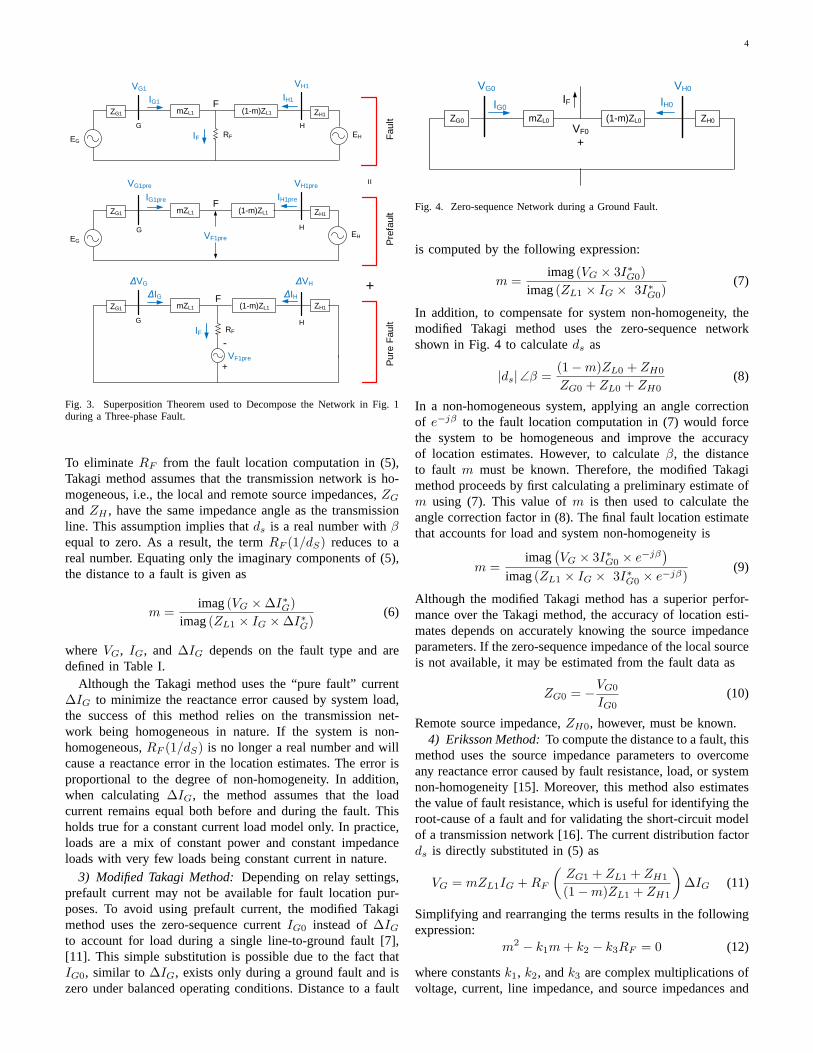
Fig. 3. Superposition Theorem used to Decompose the Network in Fig. 1during a Three-phase Fault.

To eliminateRF from the fault location computation in (5),Takagi method assumes that the transmission network is ho-mogeneous, i.e., the local and remote source impedances,ZG

andZH , have the same impedance angle as the transmissionline. This assumption implies thatds is a real number withβequal to zero. As a result, the termRF (1/dS) reduces to areal number. Equating only the imaginary components of (5),the distance to a fault is given as

m =imag(VG ×∆I∗G)

imag(ZL1 × IG ×∆I∗G)(6)

whereVG, IG, and∆IG depends on the fault type and aredefined in Table I.

Although the Takagi method uses the “pure fault” current∆IG to minimize the reactance error caused by system load,the success of this method relies on the transmission net-work being homogeneous in nature. If the system is non-homogeneous,RF (1/dS) is no longer a real number and willcause a reactance error in the location estimates. The errorisproportional to the degree of non-homogeneity. In addition,when calculating∆IG, the method assumes that the loadcurrent remains equal both before and during the fault. Thisholds true for a constant current load model only. In practice,loads are a mix of constant power and constant impedanceloads with very few loads being constant current in nature.

3) Modified Takagi Method:Depending on relay settings,prefault current may not be available for fault location pur-poses. To avoid using prefault current, the modified Takagimethod uses the zero-sequence currentIG0 instead of∆IGto account for load during a single line-to-ground fault [7],[11]. This simple substitution is possible due to the fact thatIG0, similar to∆IG, exists only during a ground fault and iszero under balanced operating conditions. Distance to a fault

IG0

mZL0 (1-m)ZL0

VG0

VF0

+

IF IH0

VH0

ZG0 ZH0

Fig. 4. Zero-sequence Network during a Ground Fault.

is computed by the following expression:

m =imag(VG × 3I∗G0

)

imag(ZL1 × IG × 3I∗G0)

(7)

In addition, to compensate for system non-homogeneity, themodified Takagi method uses the zero-sequence networkshown in Fig. 4 to calculateds as

|ds|∠β =(1−m)ZL0 + ZH0

ZG0 + ZL0 + ZH0

(8)

In a non-homogeneous system, applying an angle correctionof e−jβ to the fault location computation in (7) would forcethe system to be homogeneous and improve the accuracyof location estimates. However, to calculateβ, the distanceto fault m must be known. Therefore, the modified Takagimethod proceeds by first calculating a preliminary estimateofm using (7). This value ofm is then used to calculate theangle correction factor in (8). The final fault location estimatethat accounts for load and system non-homogeneity is

m =imag

(

VG × 3I∗G0× e−jβ

)

imag(ZL1 × IG × 3I∗G0× e−jβ)

(9)

Although the modified Takagi method has a superior perfor-mance over the Takagi method, the accuracy of location esti-mates depends on accurately knowing the source impedanceparameters. If the zero-sequence impedance of the local sourceis not available, it may be estimated from the fault data as

ZG0 = −VG0

IG0

(10)

Remote source impedance,ZH0, however, must be known.4) Eriksson Method:To compute the distance to a fault, this

method uses the source impedance parameters to overcomeany reactance error caused by fault resistance, load, or systemnon-homogeneity [15]. Moreover, this method also estimatesthe value of fault resistance, which is useful for identifying theroot-cause of a fault and for validating the short-circuit modelof a transmission network [16]. The current distribution factords is directly substituted in (5) as

VG = mZL1IG +RF

(

ZG1 + ZL1 + ZH1

(1−m)ZL1 + ZH1

)

∆IG (11)

Simplifying and rearranging the terms results in the followingexpression:

m2 − k1m+ k2 − k3RF = 0 (12)

where constantsk1, k2, andk3 are complex multiplications ofvoltage, current, line impedance, and source impedances and

5

are defined as follows:

k1 = a+ jb = 1 +ZH1

ZL1

+

(

VG

ZL1 × IG

)

k2 = c+ jd =VG

ZL1 × IG

(

1 +ZH1

ZL1

)

k3 = e+ jf =∆IG

ZL1 × IG

(

1 +ZH1 + ZG1

ZL1

)

After separating (12) into real and imaginary parts, distance tofault m can be solved from the following quadratic equation:

m =

(

a− eb

f

)

±√

(

a− eb

f

)2

− 4

(

c− ed

f

)

2(13)

wherem can take two possible values. Since the fault locationestimate must be less that the total line length, the value ofm that lies between 0 and 1 per unit should be chosen as thelocation estimate. Fault resistance can then be calculatedas

RF =d−mb

f(14)

If the local source impedanceZG1 is not available, it can becalculated from the fault event data as

ZG1 = −VG1

IG1

(15)

The remote source impedanceZH1 must be accurately known.5) Novosel et al. Method:This fault-locating technique is

a modified version of the Eriksson method and is applicablefor locating faults on a short, radial transmission line [17].All loads served by the transmission line are lumped at theend of the feeder as shown in Fig. 5. Assuming a constantimpedance load model, the first step consists of estimating theload impedance from the prefault voltage and current as

ZLoad = R+ jX =VG1pre

IG1pre

− ZL1 (16)

The per-unit distance to fault can be obtained by solving thequadratic equation in (13), where the constants are defined as

k1 = a+ jb = 1 +ZLoad

ZL1

+

(

VG

ZL1 × IG

)

k2 = c+ jd =VG

ZL1 × IG

(

1 +ZLoad

ZL1

)

k3 = e+ jf =∆IG

ZL1 × IG

(

1 +ZLoad + ZG1

ZL1

)

The value ofm which lies between 0 and 1 per unit ischosen as the location estimate. If the local source impedanceZG1 is not known, it can be estimated from (15). Similarto the Eriksson method, the Novosel et al. method is alsorobust to any reactance error due to fault resistance and load.Additional benefits include estimating the fault resistance fromthe expression in (14).

ZG

VG, IG

Terminal G

F

LoadRF IF

R

X

(1-m)ZL1mZL1

Fig. 5. Novosel et al. Method is Applicable to a Radial Transmission LineOnly. Load Model is assumed to be Constant Impedance in Nature.

B. Two-ended Impedance-based Fault Location Algorithms

Two-ended impedance-based algorithms use waveform datacaptured at both ends of a transmission line to estimate thelocation of a fault. The fault-locating principle is similar tothat of one-ended methods, i.e., using the voltage and currentduring a fault to estimate the apparent impedance from themonitoring location to the fault. Additional measurementsfrom the remote end of a transmission line are used toeliminate any reactance error caused by fault resistance, loadcurrent, or system non-homogeneity. Fault type classificationis also not required. A communication channel transfers thedata from one relay to the other. Alternatively, data from bothrelays can be collected and processed at a central location.Depending on data availability, two-ended impedance-basedmethods are further classified as follows:

1) Synchronized Two-ended Method:This method assumesthat measurements from both ends of a transmission lineare synchronized to a common time reference via a globalpositioning system (GPS). Any one of the three symmetri-cal components can be used for fault location computation.Using the negative-sequence components are, however, moreadvantageous since they are not affected by load current, zero-sequence mutual coupling, uncertainty in zero-sequence lineimpedance, or infeed from zero-sequence tapped loads [10],[18]. To illustrate the fault-locating principle, consider thenegative-sequence network during an unbalanced fault asshown in Fig. 6.VF2 is the negative-sequence voltage at thefault pointF and can be calculated from terminal G and H as

Terminal G: VF2 = VG2 −mZL2IG2 (17)

Terminal H: VF2 = VH2 − (1−m)ZL2IH2 (18)

VoltageVF2 is equal when calculated from either line terminal.Therefore, equating (17) and (18), the distance to fault (m) canbe computed as

m =VG2 − VH2 + ZL2IH2

(IG2 + IH2)ZL2

(19)

Equation 19 is applicable for locating any unbalanced faultsuch as a single line-to-ground, line-to-line, or double line-to-ground fault. However, during a three-phase balanced fault,negative-sequence components do not exist. In such a case, thesame fault-locating principle is applied to a positive-sequencenetwork and the distance to fault is computed as [19]

m =VG1 − VH1 + ZL1IH1

(IG1 + IH1)ZL1

(20)

6

ZG2 ZH2mZL2 (1-m)ZL2

VG2, IG2

IFTerminal G

VF2

+

VH2, IH2

Terminal H

Fig. 6. Negative-sequence Network during an Unbalanced Fault.

Note that there is no need to know the fault type. The presenceor absence of negative-sequence components can be used todifferentiate between an unbalanced or a balanced fault.

2) Unsynchronized Two-ended Method:Waveforms cap-tured by IED devices at both ends of a transmission line maynot be synchronized with each other. The GPS device maybe absent or not functioning correctly. Alternatively, IEDs canhave different sampling rates or they may detect the fault atslightly different time instants. The communication channel,which transfers data from one IED to the other, can alsointroduce a phase shift. Therefore, to align the voltage andcurrent measurements of terminal G with respect to terminalH, the authors in [13] use a synchronizing operatorejδ as,

Terminal G: VFi = VGiejδ −mZLiIGie

jδ (21)

Terminal H: VFi = VHi − (1−m)ZLiIHi (22)

where the subscripti refers to theith symmetrical component.As discussed in the previous subsection, negative-sequencecomponents are used to compute the location of an unbalancedfault while positive-sequence components are used to computethe location of a balanced three-phase fault. Equating (21)and(22), the synchronizing operator takes the form of

ejδ =VHi − (1−m)ZLiIHi

VGi −mZLiIGi

(23)

Now, ejδ can be eliminated mathematically from the faultlocation computation by taking the absolute value on bothsides of (23) as

∣

∣ejδ∣

∣ = 1 =

∣

∣

∣

∣

VHi − (1−m)ZLiIHi

VGi −mZLiIGi

∣

∣

∣

∣

(24)

Simplifying and rearranging the terms, the distance to fault mis a quadratic equation given by

m =−B ±

√B2 − 4AC

2A(25)

where the constants are defined as

A = |ZLiIGi|2 − |ZLiIHi|2

B = −2× Re[

VGi (ZLiIGi)∗

+ (VHi − ZLiIHi) (ZLiIHi)∗]

C = |VGi|2 − |VHi − ZLiIHi|2

Solving the quadratic equation in (25) yields two values ofm.The value between 0 and 1 per unit should be chosen as thelocation estimate.

3) Unsynchronized Current-only Two-ended Method:Dueto limitations in data availability, suppose that only the currentwaveforms at terminals G and H are available for fault locationpurposes. Voltage data is missing or unavailable. Using onlythe negative-sequence current and source impedance parame-ters,VF2 is calculated from terminals G and H as [20]

Terminal G: VF2 = − (ZG2 +mZL2) IG2 (26)

Terminal H: VF2 = − (ZH2 + (1−m)ZL2) IH2 (27)

To eliminate VF2, equate (26) with (27). Also, to avoidany alignment issues with data sets from both ends of atransmission line, consider only the absolute values as

|IH2| =∣

∣

∣

∣

(ZG2 +mZL2)

(ZH2 + (1−m)ZL2)× IG2

∣

∣

∣

∣

(28)

Squaring and rearranging the terms, the distance to faultmcan be solved by the quadratic equation in (25), where theconstants are defined as

a+ jb = IG2ZG2

c+ jd = ZL2IG2

e+ jf = ZH2 + ZL2

g + jh = ZL2

A = |IH2|2 ×(

g2 + h2)

−(

c2 + d2)

B = −2× |IH2|2 (eg + fh)− 2 (ac+ bd)

C = |IH2|2 ×(

e2 + f2)

−(

a2 + b2)

The value ofm that lies between 0 and 1 per unit shouldbe chosen as the final location estimate. This method isapplicable for locating unbalanced faults only. The accuracy oflocation estimates depends on accurately knowing the sourceimpedance parameters.

IV. EVALUATING THE SENSITIVITY OF FAULT LOCATION

ALGORITHMS TO VARIOUS ERRORSOURCES

As described in Section III, impedance-based fault loca-tion algorithms make certain simplifying assumptions whenestimating the distance to a fault. The accuracy of locationestimates deteriorates when these assumptions do not hold truedue to load, fault resistance, remote infeed, mutual couplingin parallel transmission lines, just to name a few. In addition,when computing the distance to a fault, these fault-locatingalgorithms require the input of the voltage and current phasorsduring fault as well as line impedance parameters. Inaccuracyin the input parameters further adds to the error in faultlocation. Therefore, this Section evaluates the sensitivity offault-locating algorithms to the error sources mentioned above.

A. Description of the 69-kV Test Case

To evaluate the sensitivity of impedance-based fault locationalgorithms to various sources of fault-locating error, thetwo-terminal transmission network shown in Fig. 1 was modeledin PSCAD simulation software [21]. The model will be

7

A

S1

89.25'

80'

15.5' 15.5'

8.75' 8.75'

S2

B C

Fig. 7. Tower Configuration of an Actual 69-kV Transmission Line.

used to replicate actual short-circuit faults that occur onatransmission line and generate the corresponding voltage andcurrent waveforms. The rated voltage at terminals G and H is69 kV. Relays, present at both terminals for line protection,record the three-phase line-to-ground voltages and currents at128 samples per cycle. The network upstream from terminal Gis represented by an ideal voltage sourceEG = 1∠10 per unitbehind an equivalent positive- and zero-sequence impedance ofZG1 = 3.75∠71 Ω andZG0 = 11.25∠65 Ω, respectively. Thenetwork upstream from terminal H is also represented by anideal voltage sourceEH = 1∠0 per unit behind an equivalentpositive- and zero-sequence impedance ofZH1 = 12∠71 Ωand ZH0 = 30∠65 Ω, respectively. The angle by whichEG

leadsEH is known as the power angle (δ) and representsthe net load served by the transmission line. The transmissionline connecting terminals G and H is 18 miles long and wasmodeled using the frequency dependent model in PSCAD.The tower configuration of an actual 69-kV transmission linewas used as shown in Fig. 7. Shield wires S1 and S2 protectphase conductors A, B, and C from direct lightning strikes.The material used to build the conductors is described inTable II. Using Carson’s equations [22] and an earth resis-tivity value of 100Ωm, the positive- and zero-sequence lineimpedances were calculated to beZL1 = 16.06∠70.6 Ω andZL0 = 36.01∠64.57 Ω, respectively.

Note that the test feeder has been intentionally designed tobe simple, homogeneous, and compliant with all the assump-tions made by impedance-based fault location algorithms. Thegoal is to introduce the fault-locating error sources one-by-one and study the impact on fault location estimates. Sincea simple test system is being used, the error in locationestimates is strictly proportional to the inaccuracies introduced.The analysis will, therefore, give an accurate measure of howsignificant a particular error source is and whether the errorsource should be considered for fault location purposes.

B. DC Offset and CT Saturation

Impedance-based fault location algorithms are phasor-basedalgorithms and require the input of fundamental frequencyvoltage and current phasors during a fault. Phasor calculationsare complicated by the presence of an exponentially decaying

TABLE IICONDUCTORDATA

Material Resistance Diameter GMR(Ω/mi) (inch) (feet)

Phase ACSR Linnet 336,400 26/7 0.294 0.720 0.024Shield ACSR Grouse 80,000 8/1 1.404 0.367 0.009

Fig. 8. Fault Current with a Significant DC Offset.

DC offset which makes the fault current asymmetrical duringthe first few cycles as shown in Fig. 8. The asymmetry ismaximum when a fault occurs at the zero-crossing of a voltagewaveform and minimum when a fault occurs near the voltagepeak. Fortunately, most single line-to-ground faults are causedby an animal or a tree coming in contact with a transmissionline during peak voltage condition [23]. In such cases, the DCoffset is negligible. Faults due to lightning strikes are, however,random and can occur at any point on the voltage waveform,resulting in a significant asymmetry.

To filter out the decaying DC offset and calculate the voltageand current phasors during a fault, Fast Fourier transforms(FFT) are commonly used [2]. A window length of one cycleis used to extract the fundamental-frequency magnitude andphase angle, and discard all harmonics. To illustrate the FFToperation, a rolling FFT filter is applied to the waveformin Fig. 8. In a rolling FFT, the FFT operation is performedrepeatedly by a one-cycle long window sweeping across theentire waveform. As shown in Fig. 9, the FFT operation issuccessful in filtering out most, but not all the DC offset. TheRMS magnitude of the fault current fluctuates and reachessteady-state value when the DC offset decays. The correspond-ing variation in location estimates from the simple reactancemethod is shown in Fig. 10.

Another phasor estimation technique, popularly used inSchweitzer relays, is the cosine filter [2]. Coefficients of thisfilter are sampled from a cosine wave and require a minimumresponse time of one and a quarter cycle. The quarter-cycledelay is used to calculate the phase angle. As seen in Fig. 9,the cosine filter does a better job of eliminating the DC offsetthan the FFT filter. The front and tail end of the signalare, however, severely distorted. This distortion offsetsthe

8

2 4 6 8 10 12 14 160

1

2

3

4

5

6

7

8

9

Cycles

IA R

MS

Mag

nitu

de (

kA)

Cosine FilterFFT FilterNote the response

of the FFT Filter

Fig. 9. Comparing the Effectiveness of an FFT and a Cosine Filter in Filteringout the DC Offset.

0 1 2 3 43.8

3.9

4

4.1

4.2

4.3

4.4

4.5

4.6

4.7

Cycles

Dis

tanc

e T

o F

ault

Est

imat

e (m

i)

Simple Reactance Method

Fig. 10. Variation in Location Estimates due to DC Offset. Voltage andCurrent Phasors were calculated using the FFT Filter.

accuracy of voltage and current phasor calculation duringshort-duration faults, resulting in erroneous location estimates.

In addition to DC offset, saturation of a current transformer(CT) can also distort fault current waveforms and introduceasignificant error in location estimates. CT saturation is oftencaused by fault currents having a significant DC offset [23].As the DC offset decays down within two or three cycles,the CT may stop to saturate and return to normal operation.Therefore, for faults which last for a number of cycles, thebest approach to handle CT saturation is to wait for the DCoffset to decay before applying impedance-based fault locationalgorithms.

C. Delta-connected Potential Transformers

Impedance-based fault location algorithms require the inputof line-to-ground voltages when computing the distance to afault. However, if potential transformers are connected inadelta configuration, line-to-line voltages are available instead.The measured line-to-line voltages can be used by one-ended

1/3 Line 1/3 Line 1/3 Line

Phase APhase BPhase C

Position 3

Position 2

Position 1

Fig. 11. A Transposed Transmission Line [24].

algorithms to estimate the location of line-to-line, double line-to-ground, or three-phase faults with no loss in accuracy. Line-to-ground voltages are, however, necessary to locate singleline-to-ground faults [10]. If the zero-sequence impedance ofthe source,ZGO, is available, then the line-to-ground voltageduring fault can be estimated as

VAF =1

3(VAB − VCA)− ZG0IG0 (29)

where VAF is the estimated line-to-ground voltage of thefaulted phase,VAB is the line-to-line fault voltage measuredbetween phases A and B, andVCA is the line-to-line faultvoltage measured between phases C and A. The accuracyof the estimated line-to-ground fault voltage depends on theaccuracy of the zero-sequence source impedance.

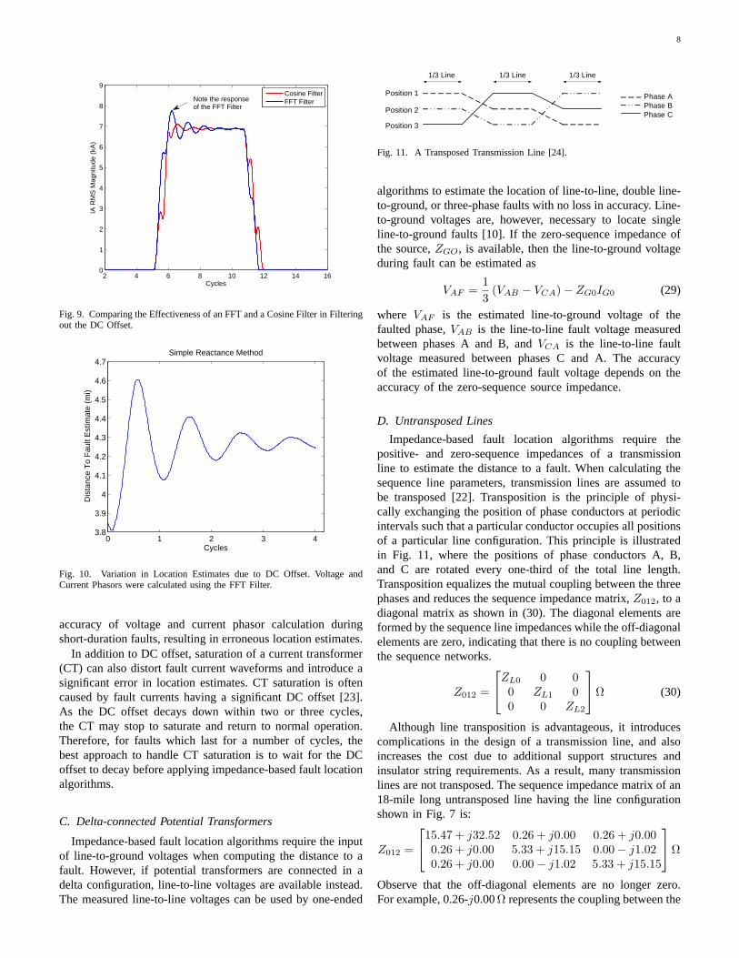
D. Untransposed Lines

Impedance-based fault location algorithms require thepositive- and zero-sequence impedances of a transmissionline to estimate the distance to a fault. When calculating thesequence line parameters, transmission lines are assumed tobe transposed [22]. Transposition is the principle of physi-cally exchanging the position of phase conductors at periodicintervals such that a particular conductor occupies all positionsof a particular line configuration. This principle is illustratedin Fig. 11, where the positions of phase conductors A, B,and C are rotated every one-third of the total line length.Transposition equalizes the mutual coupling between the threephases and reduces the sequence impedance matrix,Z012, to adiagonal matrix as shown in (30). The diagonal elements areformed by the sequence line impedances while the off-diagonalelements are zero, indicating that there is no coupling betweenthe sequence networks.

Z012 =

ZL0 0 00 ZL1 00 0 ZL2

Ω (30)

Although line transposition is advantageous, it introducescomplications in the design of a transmission line, and alsoincreases the cost due to additional support structures andinsulator string requirements. As a result, many transmissionlines are not transposed. The sequence impedance matrix of an18-mile long untransposed line having the line configurationshown in Fig. 7 is:

Z012 =

15.47 + j32.52 0.26 + j0.00 0.26 + j0.000.26 + j0.00 5.33 + j15.15 0.00− j1.020.26 + j0.00 0.00− j1.02 5.33 + j15.15

Ω

Observe that the off-diagonal elements are no longer zero.For example, 0.26-j0.00Ω represents the coupling between the

9

Fig. 12. Error in Fault Location due to Untransposed Transmission Lines.

positive- and zero-sequence network. Since impedance-basedfault location algorithms assume the sequence networks to bedecoupled from each other, an untransposed transmission lineaffects the accuracy of location estimates.

Fig. 12 demonstrates the impact of untransposed lines onone- and two-ended fault-locating techniques. In the refer-ence case (transposed line), single line-to-ground faultsweresimulated along the length of the transmission line in the69-kV test case withRF = 0Ω. Distances to faults werecomputed by applying one-ended methods to the voltage andcurrent recorded at terminal G. To apply two-ended methods,measurements captured at both terminals were used. Next, thetransmission line in the test case was intentionally changed toan untransposed line and faults were simulated with the samevalue ofRF . Distances to faults were computed using the newset of voltage and current waveforms. The fault-location errorwas calculated as

Error (%)=Actual Location− Estimated Location

Total Line Length(31)

As seen in Fig. 12, because of the line transposition assump-tion, one-ended methods underestimate the location of a faultwhen compared against the reference case. The fault-locationerror increase as faults move farther away from the monitoringlocation. Two-ended methods are also affected by the linetransposition assumption, the error being around 1.2%.

E. Uncertainty in Earth Resistivity

Earth resistivityρ is the resistance with which the earthopposes the flow of electric current. It is an electrical charac-teristic of the ground and plays a critical role when calculatingthe zero-sequence impedance of a transmission line [22].Determining the exact value ofρ is difficult since it varies

TABLE IIIVARIATION OF EARTH RESISTIVITY WITH SOIL TYPE

Soil TypeEarth Resistivity (Ωm)

Range Average

Peat >1200 200Adobe clay 2-200 40Boggy ground 2-50 30Gravel (moist) 50-3000 1000 (moist)Sand and sandy ground 50-3000 200 (moist)Stony and rocky ground 100-8000 2000Concrete: 1 part cement + 3 parts sand 50-300 150

TABLE IVEFFECT OFEARTH RESISTIVITY ON L INE IMPEDANCE PARAMETERS

ρin

crea

ses

y

ρ (Ωm) ZL1 (Ω) ZL0 (Ω)

10 5.33 +j15.15 13.59 +j30.34100 5.33 +j15.15 15.47 +j32.53500 5.33 +j15.15 16.74 +j33.871000 5.33 +j15.15 17.28 +j34.40

y ZL0

incr

ease

s

greatly with the soil type as shown in Table III. Most utilitiesuse a standard earth resistivity value of 100Ωm while othersuse the Wenner four-point method to measureρ with greataccuracy [18]. In addition to soil type, the value ofρ is alsodictated by the moisture content in soils, temperature, andseason of the year. Under extremely high or low temperatures,the soil is dry and has a very high earth resistivity value.During the rainy season, the value ofρ decreases. Minerals,salts, and other electrolytes make soils more conductive andtend to lower the earth resistivity value. Put another way, earthresistivity is never constant and is never known accurately.

Table IV shows the impact of a varying earth resistivityvalue on the positive- and zero-sequence impedances of the69-kV transmission line described in Section III. The positive-sequence line impedance remains unaffected by changes in thevalue of earth resistivity. The zero-sequence line impedance,on the other hand, increases asρ increases. Since one-ended fault location algorithms require the zero-sequencelineimpedance to compute the location of single line-to-groundfaults, these methods are sensitive to any changes in earthresistivity.

As an example, the 69-kV test case was used to demonstratethe detrimental effect ofρ on one-ended methods. Single line-to-ground faults were simulated along the entire length of thetransmission line with earth resistivity values ranging from 10to 1000Ωm. Line impedance parameters, used as an inputto the fault location algorithms, were, however, calculatedusing the standard earth resistivity value of 100Ωm. Thiscase study reflects a practical scenario in which the resistivityof the soil can indeed vary over such a wide range. However,line impedance settings in a digital relay or a fault locatorarecomputed using a particular value ofρ and does not reflectthat change. As expected, the accuracy of one-ended methodsare affected by the uncertainty in earth resistivity as shown inFig. 13. When the actual value of earth resistivity is greaterthan the one used in the fault location computation, i.e., 100Ωm, the distance to fault is overestimated. Similarly, whenρ

10

Fig. 13. Error in Fault Location due to Uncertainty in Earth Resistivity.

is lower than the value used in the fault location computation,the distance to fault is underestimated. Also observe that thefault-location error increases linearly as the fault movesfartheraway from the monitoring location. This is because the errorin the zero-sequence line impedance add up as the line lengthbetween the monitoring location and the fault increase. Incontrast, two-ended methods do not use zero-sequence lineimpedance when estimating the distance to fault and are hence,not affected by any variation inρ.

F. Effect of System Load

This subsection uses the 69-kV test case to investigate theimpact of load on the accuracy of impedance-based fault lo-cation algorithms. Single line-to-ground faults were simulatedat several locations of the 18-mile long transmission line withdifferent values of power angleδ and RF . Recall that δrepresents the net load served by the transmission network.One-ended fault location algorithms use voltage and currentcaptured at terminal G while two-ended algorithms make useof waveforms captured at either line end.

When the fault resistance is zero, location estimates fromthe simple reactance method are accurate, even during heavilyloaded conditions as shown in Fig. 14. Note that a power angleof 20 corresponds to a load current of 430 A. For non-zerovalues of fault resistance, however, the same values of loadcurrent cause a reactance error in the simple reactance method.The reactance error is capacitive and simple reactance methodunderestimates the location of faults. The fault-locationerroris further magnified when the load and fault resistance isincreased to 40 and 15Ω, respectively. It is also interestingto observe the increase in reactance error as distance to faultincreases in Fig. 14. When faults occur towards the end

0 0.2 0.4 0.6 0.8 1−40

−35

−30

−25

−20

−15

−10

−5

0

5

10

Distance to Fault (pu)

Fau

lt Lo

catio

n E

rror

(%

)

Simple Reactance Method

ρ = 20°, RF = 0 Ω

ρ = 20°, RF = 5 Ω

ρ = 20°, RF = 10 Ω

ρ = 40°, RF = 15 Ω

Reference Case

Fig. 14. Reactance Error due to Load in Simple Reactance Method.

0 0.2 0.4 0.6 0.8 1

-0.25

-0.2

-0.15

-0.1

-0.05

0

0.05

0.1

0.15

0.2

0.25

Distance to Fault (pu)

Fau

lt Lo

catio

n E

rror

(%

)

20 Degree Load, Fault Resistance 10 Ω

TakagiErikssonModified Takagi,Two-ended

Fig. 15. Load has no Impact on Takagi, Modified Takagi, Eriksson, andTwo-ended Impedance-based Fault Location Algorithms.

of the transmission line, fault current contribution from thelocal terminal decrease. Load current constitutes a significantpercent of the total fault current and increases the phaseangle mismatch betweenIF and IG. For example, when afault occurs at 0.8 per unit from terminal G, load current is28% of the fault current recorded at terminal G. As a result,the reactance error increases. Takagi method uses the “purefault” current to minimize the reactance error due to load.As shown in Fig. 15, the reactance error is negligible whenRF = 10Ω and δ = 20. Modified Takagi, Eriksson, and two-ended methods are also not affected by an increase in thesystem load.

G. Effect of a Non-homogeneous System

To demonstrate the effect of a non-homogeneous systemon impedance-based fault location algorithms, the 69-kV testcase was used. The test case is homogeneous since the localand remote source impedances have the same angle as the line

11

0 0.2 0.4 0.6 0.8 11

1.5

2

2.5

3

3.5

4

Distance to Fault (pu)

Fau

lt Lo

catio

n E

rror

(%

)

Simple Reactance Method

Homogeneous SystemNon−homogeneous System

0 0.2 0.4 0.6 0.8 1−0.5

0

0.5

1

1.5

2

2.5Takagi Method

Distance to Fault (pu)

Fau

lt Lo

catio

n E

rror

(%

)

Homogeneous SystemNon−homogeneous System

0 0.2 0.4 0.6 0.8 1−1.5

−1

−0.5

0

0.5

Distance to Fault (pu)

Fau

lt Lo

catio

n E

rror

(%

)

Eriksson Method

Homogeneous SystemNon−homogeneous System

0 0.2 0.4 0.6 0.8 1−1

−0.5

0

0.5

1

Distance to Fault (pu)F

ault

Loca

tion

Err

or (

%)

Modified Takagi and Two−ended Methods

Homogeneous System,Non−homogeneous System

Fig. 16. Effect of a Non-homogeneous System on Impedance-based Fault Location Algorithms.

impedance and hence, serves as the reference case. Single line-to-ground faults were simulated along the entire length of thetransmission line withδ = 1 and RF = 5Ω. To compute thelocation of faults, one-ended methods use voltage and currentwaveforms at terminal G while two-ended methods use voltageand current measurements at both terminals. Next, the systemis intentionally made non-homogeneous by changing the valueof ZG1 to 15∠50 Ω. Faults were simulated using the samevalues of fault resistance and load. Location estimates fromone and two-ended methods, computed using the new set ofvoltage and current measurements, were compared with thoseobtained in the reference case (homogeneous system) as shownin Fig. 16. As expected, the accuracy of simple reactanceand Takagi methods deteriorate in a non-homogeneous system.Eriksson method uses source impedance of the remote terminalto improve upon the performance of the Takagi method. Themodified Takagi and two-ended methods are also robust to theincrease in non-homogeneity and remain unaffected.

H. Zero-sequence Mutual Coupling

In transmission networks, it is common to find transmissionlines that are physically parallel to each other. Two three-phase lines may be supported by the same tower or theymay run on two separate towers but share the same rightof way. Because of mutual coupling between the two lines,the impedance to fault calculation is influenced by currentsflowing in the adjacent parallel line. This compromises theaccuracy of location estimates.

As an example, consider the double-circuit transmissionnetwork shown in Fig. 17. Rated voltage at terminals G and His 69 kV. Source impedance parametersZG andZH have the

same values as those used in Section IV-A. The transmissionline is 18 miles long and has the configuration of an actual69-kV double-circuit transmission line as shown in Fig. 18.Phase conductors A, B, and C represent Line 1 in Fig. 17while phase conductors A’, B’, and C’ represent Line 2. Thematerial used to build the conductors is the same as thosedescribed in Table II. Assuming both lines to be completelytransposed and using an earth resistivity value of 100Ωm, thesequence impedance matrixZ012 of the transmission line isshown in (32). Here, the off-diagonal term 10.52 +j25.77Ωrepresents the zero-sequence mutual coupling (Z0M ) betweentwo parallel lines and will always be present, regardless ofwhether the line is transposed or not. Observe thatZ0M issignificant, around 63% of the zero-sequence line impedance.

Now, to explain howZ0M influences impedance-basedfault location algorithms, the apparent impedance measuredat terminal G during a fault in Line 2 can be written as

Zapp =VG

IG= mZL1 +mZ0M

(

IJ0IG

)

+RF

(

IFIG

)

(33)

whereIJ0 is the zero-sequence current in the parallel trans-mission line. If two lines are parallel to each other forthe entire length of the line, thenZ0M can be taken intoconsideration by simply measuringIJ0 and inputting the valueto (33). However, many different configurations of parallellines are possible. For example, two lines may start parallelto each other from one terminal and end at two differentsubstations [25]. In such cases, the termmZ0M (IJ0/IG) willaffect the fault location calculation. If currents in parallel lines,IG and IJ , flow in the same direction, then one-ended faultlocating techniques will overestimate the location of the fault.

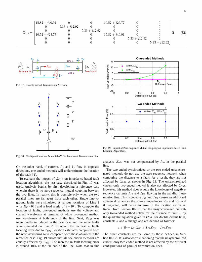
12

Z012 =

15.82 + j40.91 0 0 10.52 + j25.77 0 00 5.33 + j12.92 0 0 0 00 0 5.33 + j12.92 0 0 0

10.52 + j25.77 0 0 15.82 + j40.91 0 00 0 0 0 5.33 + j12.92 00 0 0 0 0 5.33 + j12.92

Ω (32)

Fig. 17. Double-circuit Transmission Network.

A

S

7'

50'

5'

B

C C’

B’

A’

7'

5'

5'

Fig. 18. Configuration of an Actual 69-kV Double-circuit Transmission Line.

On the other hand, if currentsIG and IJ flow in oppositedirections, one-ended methods will underestimate the locationof the fault [1].

To evaluate the impact ofZOM on impedance-based faultlocation algorithms, the test case described in Fig. 17 wasused. Analysis begins by first developing a reference casewherein there is no zero-sequence mutual coupling betweenthe two lines. In reality, this is possible only when the twoparallel lines are far apart from each other. Single line-to-ground faults were simulated at various locations of Line 2with RF = 0Ω and a load angle ofδ = 10. To compute thelocation of faults, one-ended methods use the voltage andcurrent waveforms at terminal G while two-ended methoduse waveforms at both ends of the line. Next,Z0M wasintentionally introduced in the base case and the same faultswere simulated on Line 2. To obtain the increase in fault-locating error due toZ0M , location estimates computed fromthe new waveforms were compared with those obtained in thereference case. Fig. 19 shows that all one-ended methods areequally affected byZ0M . The increase in fault-locating erroris around 10% at the far end of the line. Note that in this

Fig. 19. Impact of Zero-sequence Mutual Coupling on Impedance-based FaultLocation Algorithms.

analysis,Z0M was not compensated byIJ0 in the parallelline.

The two-ended synchronized or the two-ended unsynchro-nized methods do not use the zero-sequence network whencomputing the distance to a fault. As a result, they are notaffected byZ0M as shown in Fig. 19. The unsynchronizedcurrent-only two-ended method is also not affected byZ0M .However, this method does require the knowledge of negative-sequence currentsIJ2 and IK2 flowing in the parallel trans-mission line. This is becauseIJ2 andIK2 causes an additionalvoltage drop across the source impedancesZG andZH andif neglected, will cause an error in the location estimates.Recall from Section III-B3 that the unsynchronized current-only two-ended method solves for the distance to faultm bythe quadratic equation given in (25). For double circuit lines,constantsa andb change and are defined as follows:

a+ jb = IG2ZG2 + IJ2ZG2 − IK2ZH2

The other constants are the same as those defined in Sec-tion III-B3. It is also worth mentioning that the unsynchronizedcurrent-only two-ended method is not affected by the differentconfigurations of parallel transmission lines.

13

Fig. 20. Three Terminal Transmission Line.

I. Three-terminal Lines

Impedance-based fault location algorithms in Section IIIhave been primarily developed for a two-terminal transmissionline. The application scenario changes in the case of a three-terminal line shown in Fig. 20. One-ended fault locationalgorithms are accurate up to the tap point only. When a faultoccurs beyond the tap point, the fault current contributed bythe third terminal modifies the impedance to fault equation andresults in a significant error in location estimates. For example,consider the fault shown in Fig. 20. The apparent impedancemeasured from terminal G is:

Zapp =VG

IG= mZL1 + (m−D)ZL1

ITIG

+RF

(

IFIG

)

(34)

whereIT is the fault current contributed by terminal T andDis the distance of the tap point from terminal G. Since one-ended algorithms at terminal G have no knowledge aboutIT ,the term(m−D)ZL1 (IT /IG) will cause one-ended methodsto overestimate the location of the fault. Moreover, current IFis the summation ofIG, IH , andIT . In a non-homogeneoussystem, the phase angles of currentsIF andIG are not equaland results in an additional reactance error. Depending onwhether the reactance error is inductive or capacitive, distanceto fault is over or underestimated. On the other hand, one-ended methods can successfully estimate the location of faultF from terminal H. Since the fault is located before the tappoint, fault current contributed by terminals G and T act asremote infeed only and does not alter the apparent impedancemeasured from terminal H. Therefore, the solution in the caseof three-terminal lines is to apply one-ended methods fromeach terminal. One of the three estimates will successfullypinpoint the exact location of the fault as demonstrated in thecase study described in Section V-C.

Two-ended algorithms can be extended for application tothree-terminal lines with certain additional modifications. Forinstance, authors in [20] transform a three-terminal line intoan equivalent two-terminal line and then apply the unsynchro-nized current-only two-ended method.

J. Tapped Radial Line

Locating faults on a radial feeder tapped from a two-terminal transmission line is a challenging task for impedance-based fault location algorithms. When a fault occurs in the linesection between the tap point and the load, as illustrated byF in Fig. 21, the apparent impedance measured from terminalG is the same as that given by (34). One-ended algorithms

Fig. 21. Fault on a Radial Feeder Tapped from a Two-terminal Line.

make use of measurements captured at only one end of theline. Neglecting the fault current contributed by terminalHwill, therefore, cause one-ended methods to overestimate thefault location.

Measurements captured at both ends of a line can be usedto improve the accuracy of location estimates. The first stepisto confirm whether the fault is located on the radial line. Thisis achieved by calculating the voltage at the tap point duringfault, VTap, from terminals G and H as shown below:

Terminal G: VTap = VG −DZL1IG (35)

Terminal H: VTap = VH (36)

If the fault is on the radial line,VTap calculated from terminalG will be equal to that calculated from terminal H. This isbecause terminals G and H operate in parallel to feed thefault on the radial line. Next, (34) can be used to compute thedistance to fault.

V. A PPLICATION OF IMPEDANCE-BASED FAULT LOCATION

ALGORITHMS TO FIELD DATA

This Section demonstrates the application of impedance-based fault location algorithms on actual fault event datacaptured in utility networks. Data consists of voltage andcurrent waveforms recorded by digital fault recorders at bothends of a transmission line, line impedance parameters, andknown location of the fault. Each event was chosen to highlighta specific aspect of impedance-based fault location and toillustrate the potential benefits of IED data.

A. Utility Event 1

On 27 April 2012 at 00:48 am, a single line-to-groundfault occurred on phase A of a 161-kV transmission line.The transmission line experiencing fault is 21.15 miles longand connects Station 1 with Station 2 as shown in Fig. 22.The positive- and zero-sequence impedances of the lineareZL1 = 3.18 +j16.68Ω andZL0 = 15.21 +j52.45Ω, respec-tively. The fault was caused by a failed line arrestor located14.90 miles from Station 1 or 6.25 miles from Station 2.

Digital fault recorders (DFRs) at both stations record thethree-phase line-to-ground voltage and current waveformsat100 samples per cycle as shown in Fig. 23 and Fig. 24. Beforethe fault, Station 1 supports a load current of 150 A and Station2 supports a load current of 130 A. During the fault, the current

14

VG,IGStation 1 Fault Point F VH,IH Station 2

14.90 mi 6.25 mi

DFR DFRZG1, ZG0 ZH1, ZH0

Fig. 22. Event 1 is a A-G Fault Located 14.90 miles from Station1 or 6.25miles from Station 2

Fig. 23. Event 1 DFR Measurements at Station 1. Phase A has a Fault CurrentMagnitude of 3.4 kA.

magnitude in the faulted phase increases to 3.4 kA at Station1and 6.1 kA at Station 2. Note that to calculate the fault currentat Station 1 and 2, the third cycle after fault was chosen asthe best cycle to perform the FFT operation.

Next, to estimate the distance to fault, one-endedimpedance-based fault location algorithms were applied fromStation 1 and Station 2. The modified Takagi and Erikssonmethods require source impedance parameters as an additionalinput when computing the fault location. Therefore, waveformdata at Station 1 were used in (15) and (10) to estimatethe positive- and zero-sequence source impedances at Station1 to beZG1 = 9.4∠89 Ω andZG0 = 6.1∠90 Ω, respectively.In a similar manner, the positive- and zero-sequence sourceimpedances at Station 2 were estimated to beZH1 = 6.1∠90 Ωand ZH0 = 8.8∠81 Ω, respectively. As shown in Table V,location estimates from one-ended methods are in agreementwith those estimated by the DFRs and are close to the actuallocation of the fault.

In addition to one-ended methods, two-ended fault locationmethods were also used to estimate the distance to fault.Measurements from both ends of the transmission line areunsynchronized due to a difference in the fault trigger time.Therefore, the unsynchronized two-ended method was used.Distance to fault was computed to be 14.76 miles from Station1 as shown in Table VI.

In summary, this case study demonstrates the success ofboth one- and two-ended algorithms in tracking down the exactlocation of the fault. To further increase the benefits of fault-locating, fault event data captured at Station 1 and Station2were used to estimate the value of fault resistance. Substitutingthe estimated value ofm in (14), the fault resistance from

Fig. 24. Event 1 DFR Measurements at Station 2. Phase A has a Fault CurrentMagnitude of 6.1 kA.

TABLE VEVENT 1 LOCATION ESTIMATES FROMONE-ENDED METHODS

StationActual

Location(mi)

DFR(mi)

Estimated Location (mi)

SimpleTakagi

ModifiedEriksson

Reactance Takagi

1 14.90 14.40 14.78 14.77 14.77 14.772 6.25 6.40 6.38 6.36 6.36 6.36

TABLE VIEVENT 1 LOCATION ESTIMATE FROM TWO-ENDED METHODS

Station Actual Location Estimated Location(mi) (mi)

1 and 2 14.90 14.76

Station 1 was estimated to be 0.19Ω. Similarly, the faultresistance from Station 2 was estimated to be 0.16Ω. Theaccuracy of the estimated fault resistance can be ascertainedfrom the fact that the simple reactance method in Table Vdid not suffer from reactance error due to load current. Theabsence of any reactance error is indicative that the faultresistance is indeed negligible in this event.

B. Utility Event 2

Event 2 is a line-to-line fault that occurred between phasesA and B of a 161-kV transmission line on 25 March 2012at 03:56 pm. The transmission line is 18.63 miles long andconnects Station 1 with Station 2 as shown in Fig. 25.The positive- and zero-sequence impedances of the line areZL1 = 2.39 +j12.81Ω andZL0 = 9.95 +j40.70Ω, respectivelyand will be utilized for fault location purposes. The root-causeof the fault was a tree falling on the transmission line 2.34miles from Station 1 or 16.29 miles from Station 2.

Digital fault recorders (DFRs) at both ends of the trans-mission line capture voltage and current waveforms duringthe fault at 100 samples per cycle. The waveforms are shownin Fig. 26 and Fig. 27, and can be used to reconstruct thesequence of events. Before the fault, Station 1 and Station 2support a load current of 47 A and 55 A, respectively. When

15

2.34 mi 16.29 mi

VG,IGStation 1 Fault Point F VH,IH Station 2

DFR DFRZG1 ZH1

Fig. 25. Event 2 is a AB Fault Located 2.34 miles from Station 1 or 16.29miles from Station 2

a fault occurs 2.34 miles from Station 1, the DFR at Station1 measures a fault current of 4.8 kA in phases A and B. After3.5 cycles, a protective relay at Station 1 initiates a fast tripoperation. Station 2, on the other hand, continues to feed thefault for 34.5 cycles. During the first 3.5 cycles, when bothstations are feeding the fault, the DFR at Station 2 recordsa current magnitude of 3.2 kA in the faulted phases. This ismarked as “Part 1” in Fig. 27. After 3.5 cycles, when Station1 trips offline, the fault current from Station 2 increases to4 kA as indicated by “Part 2” in Fig. 27. After 34.5 cycles,the recloser at Station 2 operates to allow the fault to clearouton its own. The reclose interval is 2.07 seconds. The fault is,however, permanent in nature. As a result, when the reclosercloses back into the transmission line, the fault is still presentand the DFR at Station 2 records a fault current magnitude of4 kA as illustrated by “Part 3” in Fig. 27. The recloser finallylocks out after 3.5 cycles.

To track down the location of the permanent fault, one-ended impedance-based fault location algorithms were appliedfrom Station 1. Location estimates are, however, not accurateand exceed the actual location of the fault by 1.4 milesas shown in Table VII. One-ended fault location algorithmswere then applied to “Part 2” and “Part 3” of the waveformscaptured at Station 2. This is because in “Part 2” and “Part3”, only Station 2 contributes current to the fault. There isno remote infeed from Station 1 and hence, location estimatesare expected to have a high degree of accuracy. Unfortunately,as seen in Table VII, one-ended methods from Station 2 alsooverestimate the location of the fault by 1.9 miles. It should benoted that in addition to the one-ended methods, the DFRs atStation 1 and Station 2 also incorrectly identify the locationof the fault. To explain the fault location error, recall thatthe Eriksson method is robust to fault resistance, load, anda non-homogeneous system. Erroneous estimates from theEriksson method, therefore, rules out the above sources offault-locating error. Moreover, since the fault does not involvethe ground, zero-sequence mutual coupling and uncertaintyin zero-sequence line impedance can also be eliminated aspotential error sources. Additional information regarding thetransmission network is required to identify the factor respon-sible for the error in fault location.

Fault location estimate from the unsynchronized two-endedmethod is summarized in Table VIII. Since the DFRs atStation 1 and Station 2 have different fault trigger times, theunsynchronized two-ended method was chosen and appliedto that part of the waveform wherein both stations are con-tributing to the fault, i.e., Station 1 and “Part 1” of Station 2waveform. As seen from the table, location estimate from thetwo-ended method show a significant improvement over one-

Fig. 26. Event 2 DFR Measurements at Station 1. Fault Current Magnitudein Phases A and B is 4.8 kA.

Fig. 27. Event 2 DFR Measurements at Station 2.

TABLE VIIEVENT 2 LOCATION ESTIMATES FROMONE-ENDED METHODS

StationActual

Location(mi)

DFR(mi)

Estimated Location (mi)

Simple Reactance Takagi Eriksson

1 2.34 3.90 3.77 3.77 3.782, Part 2

16.29 18.0018.08 18.08 18.04

2, Part 3 18.18 18.18 18.16

ended methods and is within 0.15 miles of the actual faultlocation.

In addition to estimating the location of the fault, voltageandcurrent waveforms captured during the fault provide valuablefeedback about the state of the transmission network upstreamfrom the DFR at Station 1 and Station 2. For example, toimplement the Eriksson method in Table VII, waveform dataat each individual station were used in (15) to estimate thesource impedance parameters listed in Table IX. Observe thesudden change in the positive-sequence source impedanceat Station 2 from “Part 1” to “Part 2”. Keep in mind thatthe fault current contribution from Station 2 lasts for 34.5cycles. Several generators upstream from Station 2 must haveswitched offline during this long time frame, resulting in asharp decrease in the source impedance.

16

TABLE VIIIEVENT 2 LOCATION ESTIMATE FROM TWO-ENDED METHODS

Station Actual Location Estimated Location(mi) (mi)

1 and 2 2.34 2.46

TABLE IXESTIMATED POSITIVE-SEQUENCESOURCE IMPEDANCES

Station Source Impedance

1 1.85 +j14.462, Part 1 4.25 +j12.802, Part 2 6.46 +j6.292, Part 3 3.19 +j7.22

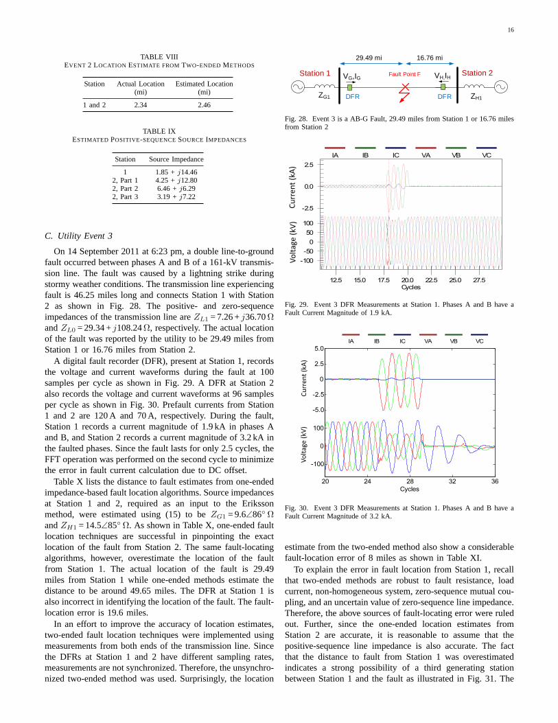
C. Utility Event 3

On 14 September 2011 at 6:23 pm, a double line-to-groundfault occurred between phases A and B of a 161-kV transmis-sion line. The fault was caused by a lightning strike duringstormy weather conditions. The transmission line experiencingfault is 46.25 miles long and connects Station 1 with Station2 as shown in Fig. 28. The positive- and zero-sequenceimpedances of the transmission line areZL1 = 7.26 +j36.70ΩandZL0 = 29.34 +j108.24Ω, respectively. The actual locationof the fault was reported by the utility to be 29.49 miles fromStation 1 or 16.76 miles from Station 2.

A digital fault recorder (DFR), present at Station 1, recordsthe voltage and current waveforms during the fault at 100samples per cycle as shown in Fig. 29. A DFR at Station 2also records the voltage and current waveforms at 96 samplesper cycle as shown in Fig. 30. Prefault currents from Station1 and 2 are 120 A and 70 A, respectively. During the fault,Station 1 records a current magnitude of 1.9 kA in phases Aand B, and Station 2 records a current magnitude of 3.2 kA inthe faulted phases. Since the fault lasts for only 2.5 cycles, theFFT operation was performed on the second cycle to minimizethe error in fault current calculation due to DC offset.

Table X lists the distance to fault estimates from one-endedimpedance-based fault location algorithms. Source impedancesat Station 1 and 2, required as an input to the Erikssonmethod, were estimated using (15) to beZG1 = 9.6∠86 ΩandZH1 = 14.5∠85 Ω. As shown in Table X, one-ended faultlocation techniques are successful in pinpointing the exactlocation of the fault from Station 2. The same fault-locatingalgorithms, however, overestimate the location of the faultfrom Station 1. The actual location of the fault is 29.49miles from Station 1 while one-ended methods estimate thedistance to be around 49.65 miles. The DFR at Station 1 isalso incorrect in identifying the location of the fault. Thefault-location error is 19.6 miles.

In an effort to improve the accuracy of location estimates,two-ended fault location techniques were implemented usingmeasurements from both ends of the transmission line. Sincethe DFRs at Station 1 and 2 have different sampling rates,measurements are not synchronized. Therefore, the unsynchro-nized two-ended method was used. Surprisingly, the location

VG,IGStation 1 Fault Point F VH,IH Station 2

DFR DFRZG1 ZH1

29.49 mi 16.76 mi

Fig. 28. Event 3 is a AB-G Fault, 29.49 miles from Station 1 or 16.76 milesfrom Station 2

Fig. 29. Event 3 DFR Measurements at Station 1. Phases A and B have aFault Current Magnitude of 1.9 kA.

Fig. 30. Event 3 DFR Measurements at Station 1. Phases A and B have aFault Current Magnitude of 3.2 kA.

estimate from the two-ended method also show a considerablefault-location error of 8 miles as shown in Table XI.

To explain the error in fault location from Station 1, recallthat two-ended methods are robust to fault resistance, loadcurrent, non-homogeneous system, zero-sequence mutual cou-pling, and an uncertain value of zero-sequence line impedance.Therefore, the above sources of fault-locating error were ruledout. Further, since the one-ended location estimates fromStation 2 are accurate, it is reasonable to assume that thepositive-sequence line impedance is also accurate. The factthat the distance to fault from Station 1 was overestimatedindicates a strong possibility of a third generating stationbetween Station 1 and the fault as illustrated in Fig. 31. The

17

TABLE XEVENT 3 LOCATION ESTIMATES FROMONE-ENDED METHODS

StationActual

Location(mi)

DFR(mi)

Estimated Location (mi)

Simple Reactance Takagi Eriksson

1 29.49 49.10 49.27 49.43 49.652 16.76 16.60 16.68 16.66 16.65

TABLE XIEVENT 3 LOCATION ESTIMATE FROM TWO-ENDED METHODS

Station Actual Location Estimated Location(mi) (mi)

1 and 2 29.49 37.41

VG,IGStation 1 Fault Point F VH,IH Station 2

DFR DFRZG1 ZH1

29.49 mi 16.76 mi

Station 3

Possible 3rd Generator

I T

Fig. 31. A Third Station is Suspected to be Present Between Station 1 andthe Fault

fault current from Station 3 increases the apparent impedancemeasured at Station 1. As a result, one- and two-endedalgorithms overestimate the location of the fault from Station1. As discussed in Section III, in a three-terminal line, one-ended fault location estimates computed from only one of thethree terminals, Station 2 in this case, is accurate.

As an added benefit to fault-locating, waveforms at Station2 were used in (14) to estimate the fault resistance as 0.87Ω.Waveforms from Station 1 were not used since the fault currentfrom Station 3 modifies the fault resistance calculation.

VI. L ESSONSLEARNED

This paper reviews one- and two-ended impedance-basedfault location algorithms that are used to locate faults in atransmission network. The simple reactance method is thesimplest of all fault location algorithms. The accuracy of thismethod, however, deteriorates due to fault resistance, loadcurrent, and remote infeed in a non-homogeneous system.Subsequent fault-locating algorithms developed in the liter-ature focus on addressing the above sources of error. Forexample, Takagi method is robust to load but sensitive toremote infeed. The modified Takagi and Eriksson methods usesource impedance parameters to eliminate any error causedby load and remote infeed. Additional sources of error thatcompromise the accuracy of one-ended algorithms in locatingsingle line-to-ground faults are mutual coupling in double-circuit transmission lines and an uncertain value of zero-sequence line impedance. Two-ended fault-locating algorithmsuse measurements from both ends of a transmission lineto overcome all the short-comings of one-ended methods

and are attractive for use in fault location. Unfortunately,measurements captured at the remote end of the line are notalways available. Therefore, data available for fault locationis one of the most important criteria for selecting the best ap-proach for fault location. Table XII summarizes the input datarequirement of all impedance-based fault location algorithms.

Identifying the best approach for fault location also dependson the application scenario. For example, location estimatesfrom two-ended algorithms are not always accurate as in thecase of three-terminal lines demonstrated in Section V-C. Incontrast, one-ended fault locating algorithms applied fromone of the three terminals pinpoints the exact location ofthe fault. The two-ended fault location algorithm failed notbecause of limitations in the algorithm but because it wasnot meant for use in a three-terminal line. Therefore, whenimplementing fault location algorithms, users should be awareof the application scenario, identify possible error sources,and then choose the algorithm that is robust to those errorsources. Table XIII summarizes the error sources that affectthe accuracy of impedance-based fault location algorithms.

Knowing the fault location application scenario is alsouseful in identifying what additional equipment needs to beinstalled for improving the accuracy of fault location algo-rithms. For instance, locating faults on a radial line tappedfrom a multi-ended transmission line is a complex problemas discussed in Section IV-J. Placing an additional monitoratthe tap point in Fig. 21 would drastically simplify impedance-based fault location.

In addition to computing the location of a fault, this paperdemonstrates the other potential benefits of event reportscaptured by intelligent electronic devices (IEDs) during afault. For example, fault event data can be used to determinethe Thevenin impedance upstream from the IED device. Theestimated Thevenin impedance can yield valuable clues aboutthe response of the upstream transmission network during thefault, including whether any generators have tripped offline.Fault event data can also be used to estimate the value of faultresistance, which is useful for identifying the root cause of thefault and also for validating system modeling parameters.

In summary, the paper recommends the following criteriafor selecting the most suitable fault location algorithm: (a)data available for fault location, (b) fault location applicationscenario. Utility operators should also remember that whenestimating the distance to a fault, fault location algorithmsassume that only one fault occurs in the transmission line atagiven point in time and that the location of the fault remainsthe same for the entire duration of the fault-locating window.Faults caused by animal or tree contact with a transmissionline, or insulation failure in power system equipment have onesingle location. However, when lightning strikes an overheadline or a shield wire, the voltage across the insulator isso large that it causes a back flash-over and a fault. Thisovervoltage may propagate to the neighboring towers andcause simultaneous flash-overs at several locations. In thiscase, the fault is not limited to one single location and canchallenge the application of impedance-based fault locationalgorithms.

18

TABLE XIISUMMARY OF INPUT DATA REQUIREMENT OFIMPEDANCE-BASED FAULT LOCATION ALGORITHMS

Input DataSimple

Reactance TakagiModifiedTakagi Eriksson

Novoselet al.

SynchronizedTwo-ended

UnsynchronizedTwo-ended

UnsynchronizedCurrent-only Two-ended

Fault Data

Fault Type

Fault Voltage1, CurrentPhasor (Local End)

Fault Voltage Phasor1

(Remote End)

Fault Current Phasor(Remote End)

Synchronized Data

Prefault Current Phasor

Prefault Voltage Phasor

Line Parameters

Line Length

Positive-sequenceLine Impedance

Zero-sequenceLine Impedance

Source Impedance Parameters

Positive-sequence SourceImpedance (Local End) Optional Optional

Positive-sequence SourceImpedance (Remote End)

Negative-sequence SourceImpedance (Local End)

Negative-sequence SourceImpedance (Remote End)

Zero-sequence Source2

Impedance (Local End)Optional

Zero-sequence SourceImpedance (Remote End)

1 Voltages refer to line-to-ground voltages.2 If line-to-line voltages are available, the zero-sequencesource impedance at the local end is required to estimate the line-to-ground voltage.

19

TABLE XIIISUMMARY OF FAULT-LOCATING ERRORSOURCES THATAFFECT IMPEDANCE-BASED FAULT LOCATION ALGORITHMS

Input DataSimple

Reactance TakagiModifiedTakagi Eriksson

Novoselet al.

SynchronizedTwo-ended

UnsynchronizedTwo-ended

UnsynchronizedCurrent-only Two-ended

Instrument Transformer Challenges

Loss of Potential

CT Saturation

Delta-connectedPotential Transformers1

Power System Challenges

System Load

Non-homogeneous System

Parallel Lines2

(Mutual Coupling)

Fault Related Challenges

Fault Resistance

Fault Incidence Angle(DC Offset)

Application Related Challenges

Two Terminal Line N/A

Soil Type, WeatherTemperature, Season(Earth Resistivity)

Untransposed Line

Tapped Lines3

Three-Terminal Line3

1 If the zero-sequence impedance of the local source is available, estimate the line-to-ground voltages.2 If transmission lines are parallel for the entire line length, residual current from the parallel line can improve the accuracy of one-ended methods.

The unsynchronized current-only two-ended method requiresthe negative-sequence currents at both ends of the parallelline.3 It is possible to modify two-ended methods for application to tapped lines and three-terminal lines.

20

ACKNOWLEDGMENT

The authors would like to thank “Mr. TVA person” formaking real-world data available for the analysis in this paper.They would also like to thank Mr. Nate Herbert for his helpin proofreading the paper.

REFERENCES

[1] “IEEE guide for determining fault location on AC transmission anddistribution lines,”IEEE Std C37.114-2004, pp. 1 –36, 2005.

[2] Distribution fault location: field data and analysis, EPRI, Palo Alto,CA: 2006. 1012438.

[3] S. Lotfifard, M. Kezunovic, and M. Mousavi, “A systematic approachfor ranking distribution systems fault location algorithms and eliminatingfalse estimates,”IEEE Transactions on Power Delivery, vol. 28, no. 1,pp. 285–293, Jan 2013.

[4] M. M. Saha, R. Das, P. Verho, and D. Novosel, “Review of faultlocation techniques for distribution systems,” inPower Systems andCommunications Infrastructures for the Future, September 2002.

[5] J. Mora-Florez, J. Melendez, and G. Carrillo-Caicedo, “Comparison ofimpedance based fault location methods for power distribution systems,”Electric Power Systems Research, vol. 78, no. 4, pp. 657 – 666, 2008.

[6] M. Mirzaei, M. Z. A. A. Kadir, E. Moazami, and H. Hizam, “Review offault location methods for distribution power system,”Australian Journalof Basic and Applied Sciences, 2009.

[7] R. Zivanovic, “Evaluation of transmission line fault-locating techniquesusing variance-based sensitivity measures,” in16th Power System Com-putation Conference, July 2008, pp. 1–6.

[8] M. Hashim, H. W. Ping, and V. Ramachandaramurthy, “Impedance-based fault location techniques for transmission lines,” inIEEE Region10 Conference, TENCON, Jan 2009, pp. 1–6.

[9] A. L. Dalcastagne and S. L. Zimath, “A study about the sources of errorof impedance-based fault location methods,” inIEEE/PES Transmission& Distribution Conference and Exposition: Latin America, 2008, pp.1–6.

[10] E. O. Schweitzer III, “A review of impedance-based faultlocatingexperience,” in14th Annual Iowa-Nebraska System Protection Seminar,October 1990.

[11] K. Zimmerman and D. Costello, “Impedance-based fault location ex-perience,” inProc. 58th Annual Conf. for Protective Relay Engineers,April 2005, pp. 211 – 226.

[12] V. Nunez, S. Kulkarni, S. Santoso, and M. Joaquim, “Feature analysisand classification methodology for overhead distribution fault events,” inIEEE Power and Energy Society General Meeting, July 2010, pp. 1–8.

[13] M. M. Saha, J. J. Izykowski, and E. Rosolowski,Fault location on powernetworks, 1st ed. Springer, 2010.

[14] T. Takagi, Y. Yamakoshi, M. Yamaura, R. Kondow, and T. Matsushima,“Development of a new type fault locator using the one-terminal voltageand current data,”IEEE Trans. on Power Apparatus and Systems, vol.PAS-101, no. 8, pp. 2892 –2898, Aug. 1982.

[15] L. Eriksson, M. M. Saha, and G. D. Rockefeller, “An accurate faultlocator with compensation for apparent reactance in the fault resistanceresulting from remote-end infeed,”IEEE Trans. on Power Apparatusand Systems, vol. PAS-104, no. 2, pp. 423–436, 1985.

[16] Transmission Line Protection Support Tools: Fault Location Algorithmsand the Potential of Using Intelligent Electronic Device Data forProtection Applications, EPRI, Palo Alto, CA: 2013. 3002002381.

[17] D. Novosel, D. Hart, Y. Hu, and J. Myllymaki, “System for locatingfaults and estimating fault resistance in distribution networks with tappedloads,” US Patent Number 5839093, November 17, 1998.

[18] A. Amberg, A. Rangel, and G. Smelich, “Validating transmission lineimpedances using known event data,” in65th Annual Conference forProtective Relay Engineers, April 2012, pp. 269–280.

[19] E. O. Schweitzer III, “Evaluation and development of transmission linefault-locating techniques which use sinusoidal steady-state information,”Computers & Electrical Engineering, vol. 10, no. 4, pp. 269–278, 1983.

[20] D. A. Tziouvaras, J. B. Roberts, and G. Benmouyal, “New multi-ended fault location design for two- or three-terminal lines,” in SeventhInternational Conference on Developments in Power System Protection,(IEE), 2001, pp. 395–398.

[21] Applications of PSCAD®/EMTDCTM, Manitoba HVDC Research CenterInc., Manitoba, Canada.

[22] W. H. Kersting, Distribution System Modeling and Analysis, 3rd ed.CRC Press, 2012.

[23] T. A. Short,Electric Power Distribution Handbook. CRC Press, 2004.

[24] R. E. Fehr, “Sequence impedances of transmission lines,”May, 2004.[25] A. Apostolov, D. Tholomier, S. Sambasivan, and S. Richards, “Protec-

tion of double circuit transmission lines,” in60th Annual Conference forProtective Relay Engineers, March 2007, pp. 85–101.

Swagata Dasreceived the B.Tech. degree from SRM University, India in2009 and the M.S.E degree from the University of Texas at Austin in 2011,both in electrical engineering. She is currently pursuing her Ph.D. in ElectricalEngineering from the University of Texas at Austin.

Her research interests are in fault location, power quality, and smart gridtechnologies.

Surya Santosoreceived the B.S degree from Satya Wacana Christian Uni-versity, Salatiga, Indonesia, in 1992, and the M.S.E. and Ph.D. degrees inelectrical engineering from the University of Texas at Austin in 1994 and1996, respectively.

From 1997 to 2003, he was a Consulting Engineer with ElectrotekConcepts. Currently, he is an Associate Professor in the Department ofElectrical and Computer Engineering at the same university. His researchinterests include power quality, power systems, and wind power.

Anish Gaikwad is a Project Manager in Grid Operations and Planninggroup at Electric Power Research Institute (EPRI). His current activities focuson EPRIs research projects related to transmission planning. He is leadingEPRIs research efforts on developing advanced planning tools for transmissionnetwork analysis and risk-based planning.

His main areas of interest are modeling and model validation fortransmis-sion planning studies, risk-based transmission planning, interconnection stud-ies, transient studies and insulation coordination. He is involved in distributionstudies related to Conservation Voltage Reduction, improving distributionefficiency and modeling and analysis related to distributionsystems.

Mahendra Patel ......