Imperfect Competition and Sanitation:

Evidence from randomized auctions in Senegal∗

Jean-Francois Houde Terrence Johnson

UW-Madison University of Virginia

& NBER

Molly Lipscomb Laura Schechter

University of Virginia UW-Madison

November 2, 2020

∗Preliminary and Incomplete. We thank Madelyn Bagby, Josh Deutschman, Jared Gars, Shoshana Griffith,Ahmadou Kandji, Nitin Krishnan, Sarah Nehrling, and Cheikh Samb for excellent research assistance and the Billand Melinda Gates Foundation for generous funding for the project. Thanks to Mbaye Mbeguere and the membersof the Senegal Office of Sanitation (ONAS) as well as Water and Sanitation for Africa for their collaboration on thisproject. We thank Radu Ban, Lori Beaman, Charlie Holt, Seema Jayachandran, Cynthia Kinnan, Robert Porter, MarReguant, seminar participants at the Econometrica Society North American Winter Meetings, Dartmouth, NBER-Market Design Fall Meetings, Northwestern University, Princeton University, University of Michigan, University ofVirginia, UW-Madison, UW-Milwaukee, and the Washington-Area Development Conference for their comments.

1

Introduction

An important problem affecting markets in developing countries is the lack of antitrust oversight.

To the extent that this enable firms to more easily coordinate prices and exert market power, this

is an important impediment to growth and resource allocation.1 In the context of products and

services that have the potential to reduce negative externalities, the welfare cost of market power is

even more severe. In sanitation markets, such as the removal of domestic waste, the under-provision

of clean technologies adversely affects water and air quality, and increases the risk of health-related

problems.

In this paper, we analyze the importance of imperfect competition and collusion in the market

for sanitation services in Dakar, Senegal. As a consequence of rapid urbanization and under-

investment in public infrastructure, most peri-urban areas of Dakar are not connected to a sewage

network system. Instead, households rely on individual sanitation systems such as septic tanks and

unimproved pits. These systems need to be emptied periodically (on average twice per year); a

service that we refer to as desludging. Households choose between two options: manual workers

who enter the pit and extract the sludge using shovels and buckets and dump the sludge in the

street; and truckers capable of pumping the sludge and then taking it out of the neighborhood,

usually to one of three treatment centers. Survey evidence suggests that slightly more than half

of desludgings are performed using the manual option, which creates important environmental and

health externalities (Deutschman et al. 2016).

Competition between firms is limited by the presence of a trade association (AAAS). The

Association is controlled by the largest companies active in the market, which together control

directly or indirectly roughly 50% of trucking capacity. The role of the association is to coordinate

equipment purchases and bid on non-residential desludging contracts. The leaders of the association

also control the prices set in the main garages where truckers park and meet residential clients. This

limits competition both within and across neighborhoods of the city. The effect of the association on

prices is illustrated by the difference between neighborhoods controlled by AAAS, and a submarket

(Rufisque) dominated by unaffiliated companies. Companies in Rufisque use a posted-price schedule

(as opposed to price negotiation), and charge mechanical prices that are 40% lower on average than

in the rest of the city. As a result, over 90% of the population in the competitive area use mechanical

desludging over the manual options (compared to 40% in the rest of the city), and companies operate

at near full capacity.

Our objective is to measure the extent to which firms behave competitively in this market, by

studying their pricing strategies in over 5,000 randomized auction experiments. The data comes

from a real-time auction platform that we designed in partnership with the State government to

improve access to desludging services. Starting in the fall of 2013, households in all neighborhoods

of Dakar were able to obtain a quote for mechanical desludging by contacting a call center. Suppliers

1See for instance Aghion and Griffith (2005) and Asker, Collard-Wexler, and De Loecker (2019).

1

were invited to bid anonymously by sending text messages to the platform, and the lowest bid was

presented to the client, who had the option to accept or reject (the average acceptance frequency is

30%). Although not perfectly comparable, this process of generating offers is similar to how many

clients find truckers. On average, 63% of households report finding providers by calling directly the

driver, or using a reference from a friend or family member. The platform facilitates this process

by allowing consumers to use an intermediary to collect multiple offers simultenously.

Two sources of randomization were introduced in the design of the auctions. When a client

calls, he/she is assigned to a randomly selected group of potential bidders ranging from 8 to 20. In

addition, the format of the auctions is itself random across clients. In 50 percent of auctions, the

platform uses a revisable format which provides information about the current lowest-standing bid

received, and allowed bidders to revise their bid (as in Hortacsu and Kastl (2012)). The remaining

auctions are conducted using a sealed-bid format.

We use random variation across formats and invitation lists to test the null hypothesis that

invited bidders behave competitively in the platform. Since each auction is anonymous and per-

formed over a short period of time (60 minutes), the platform offers an opportunity for truckers

to generate more revenues, and break from collusion. To test this hypothesis, we first identify

strategies that are inconsistent with competitive bidding (e.g. Porter and Zona (1993), Porter and

Zona (1999), Chassang et al. (2019)). An action is defined as “non-competitive” if bidders fail to

maximize expected profit in an effort to suppress competition. This identification strategy relies on

documenting the prevalence of strategies that are either dominated and dominant for all bidders,

irrespectively of their cost. We focus on two types of dominated actions that are specific to each

auction format.

The first is the propensity of bidders to avoid ties in sealed-bid auctions. Focal prices are

common in the market, since most transactions are cash-based. Targeting focal prices used in

the residential market leads to a high probability of observing ties in the auctions (20%). This

softens competition by turning the auction into a lottery and allocating the good to participants

who submit early bids. This is a dominated strategy from the point of view of a profit maximizing

bidder.

The second strategy is the propensity of bidders to submit a late bid in the revisable auction

format. In this format, bidders are informed about the current lowest bid, and have the option of

submitting a sealed bid in the last 10 minutes of each auction. Assuming private values, bidding

in the closed portion of the revisable auction is a dominant strategy. Since winning bidders pay

their bid, it is optimal for firms to wait until after the last message before submitting a bid. Doing

so limits the likelihood that the bid is undercut, and to the extent that bidding is costly, firms are

better off learning about rival bids before submitting a bid. In contrast, submitting an early bid

can be viewed as an effort to coordinate prices by sending a signal to rivals.

Our results suggest that the market is composed of a small group of profit maximizing bidders

(roughly 1/3), competing with a larger group of firms whose behavior is inconsistent with compet-

2

itive bidding. We show that the frequency of ties and early winning bids is reduced significantly

when auctions are conducted using the revisable format (compared to sealed), implying that the

market includes a group of competitive bidders. However, the overall fraction of dominated actions

is positive in both formats, suggesting that a number of bids are non-competitive.

In addition, we show that there exists a strong positive correlation between firm conducts

across formats. In particular, bidders who are likely to tie in the sealed-bid auctions are also

submitting lower bids on average, and are more likely to bid late and undercut other bidders in

the revisable auctions. This implies that the presence of non-competitive bids is not due to bidders

committing random errors or inattentions across auctions: Non-competitive bidders systematically

use dominated strategies (and conversely for competitive bidders). Crucially, we obtain this result

by comparing frequent bidders in the auctions, which reduces the importance of learning or insincere

bidding as alternatively interpretations for these result

Having established that the market is not competitive, we evaluate the potential damages from

collusion by measuring the counter-factual demand for mechanical desludging under the assumption

that households had access to more competitive price distributions. We consider two competitive

scenarios: (i) the observed distribution of prices in the Rufisque neighborhood, and (ii) the auction

price distribution under more competitive invitation lists. The results show that demand would

increase substantially in both cases: from 42% to 71% using Rufisque prices, and to 54% using

the auctions. These two experiments are partial equilibrium simulations, that do not account for

changes in bidding strategies if all transactions were conducted using the auction platform. In

a companion paper, Houde et al. (2020), we use the auction data to estimate the distribution of

desludging cost, and simulate the equilibrium effect of eliminating non-competitive strategies and

using competitive invitation lists.

Our paper is part of a growing set of papers using tools from Industrial Organization to study

the functioning of markets in developing countries (e.g. Keniston (2011), Allcott, Collard-Wexler,

and O’Connell (2018), Bjorkegren (2019), Ryan (Forthcoming)). Among those, our paper is closest

to two recent papers studying market frictions using data from field experiments. Falcao Bergquist

and Dinerstein (2019) analyze market power in a wholesale market for agricultural products in

Kenya. The paper uses a field-experiment to analyze the pass-through of cost shocks on prices

and demand, and identify a model of imperfect competition. Johnson and Lipscomb (2020) uses

market-design tools to evaluate the optimal targeted subsidies for improved sanitation in Burkina

Faso.

Our paper also contributes to the literature on diagnostic tests for collusion.2 There are two

strands of literature studying collusion. The first one relies on testing implications of efficient models

collusions. Examples of this approach include Bresnahan (1987) in an oligopoly market context,

and Baldwin, Marshall, and Richard (1997), Bajari and Ye (2003), Asker (2010) in auction markets.

2See Hendricks and Porter (1989), Porter (2005) and Abrantes-Metz and Bajari (2009) for discussions of thisliterature.

3

Ale-Chilet and Atal (Forthcoming) uses this approach study the role of a trade association in Chile

in facilitating collusion. The second identifies strategies that are inconsistent with competitive

behavior (e.g. Porter and Zona (1993), Porter and Zona (1999), Chassang et al. (2019)). We follow

the second approach here by identifying bids that violate assumptions about competitive behavior.

The paper is also connected to the literature studying behavioral biases by firms in strategic

environments (see Della Vigna (2018) for a review). Failure to maximize individual profit can arise

also for other reasons than limiting competition. For instance, Hortacsu et al. (2019) identifies the

importance of bounded-rationality in electricity auctions, assuming competitive bidding. Although

we cannot rule out completely that sub-optimal bids are caused bounded-rationality (as opposed

to tacit collusion), our results similarly show that an increase in the fraction of bidders avoiding

dominated strategies can lead to important efficiency gains. Similarly, as in Doraszelski, Lewis,

and Pakes (2018), we show that bidders quickly learn how to behave strategically in a new auction

environment.

The rest of the paper is organized as follows. We first describe the data and the structure of the

market. We take a first look at the importance of collusion by analyzing the distribution of prices

between areas that are controlled by the association, compared to our competitive control. The

next section analysis non-competitive behavior in the auction platform. The final section evaluates

the effect of imperfect competition on demand and consumer surplus.

1 Data

We use three datasets to conduct our empirical analysis: (i) a household survey of technology choice

and price, (ii) a provider survey, and (iii) administrative data from the just-in-time auctions.

We conducted four sets of household surveys spanning November 2012-June 2015. We inter-

viewed 9,672 households, randomly selecting some neighborhoods for repeat interviews to create

a panel dataset, generating 16,255 observations in total. We drop observations with missing re-

sponses on key variables including those who did not receive a desludging over the past year (either

mechanical or manual). The final sample size includes 7,824 observations, and 5,242 unique house-

holds.3 We use the household surveys to measure the distribution of prices and demand across

neighborhoods. An observation corresponds to a household’s most recent desludging transaction.

We constructed our random sample of households from areas farther removed from the sewage

network, using geographic sampling techniques: we overlaid grid points on a map of Dakar, dropped

grid points which were in uninhabited areas or served by the city sewer network, randomly selected

grid points for sampling from the remaining points, and used a spiral method to select households

for the sample starting from each randomly selected neighborhood grid point. Figure 12 in the

Appendix displays the distribution of households’ locations. Our analysis focuses on five of the 19

3Some households were surveyed over multiple years in order to measure their response to a direct subsidy program(or serve as a control group). Households who were part of the subsidy intervention program are excluded from ourdata.

4

Arrondissements of Dakar.4 The majority of households surveyed are located in five neighborhoods:

Pikine Dagoudane (center-west, 14%), Thiaroye (center, 30%), Guediawaye (center-east, 13.5%),

Niayes (north-east, 37%), and Rufisque (south-east, 4.8%). Note that households in Rufisque were

not sampled in the second and third wave of the surveys, which explains the smaller number of

observations (i.e. 250 unique households).5

On the firm side, we conducted a baseline survey covering 121 desludging truck operators in

May and June 2012, and an endline survey of 152 drivers (of which 13 owned their own truck), 75

truck-owners, and 20 managers were surveyed in June 2015. We refer to an operator either as a

manager of a fleet of trucks, or a driver associated with a single license plate. These two surveys

include data from several truck operators who decided not to participate in the auction platform

as well as most operators associated with the call center. In addition, we also collected information

on the truck size and location of most license plates active in the market (≈ 350). We use the

provider survey to identify the main location of each truck in the market to measure the distance

between households and truckers.

Finally, we use data from a just-in-time auction platform for the procurement of residential

desludging jobs. Together with Water and Sanitation for Africa (WSA) and the National Office

of Sanitation in Senegal (ONAS), we ran the call-center from July 2013-September 2015. The call

center has since been scaled up by ONAS. Call center activity is clustered around the peri-urban

areas of Dakar, particularly Pikine and Guediawaye, but calls have come from downtown Dakar as

well as further out of the city.

We have access to the administrative data from these auctions: the identities of the desludgers

who were invited to bid (invitations were randomized), whether or not they bid, the time and

amount of their bid if they made one, the format of the auction (auction format was randomized),

the location of the household job that they were bidding on, and the winning bid.

2 Residential desludging in Dakar

In this section, we describe the functioning of the residential market for desludging in Dakar.

Section 3.1 describes the functioning of the call center.

2.1 Demand

When a household latrine fills, the household must empty it (getting a desludging) in order to

restore it to working order. Households have a choice between three types of desludging services:

(i) manual, performed by a family member, (ii) manual, performed by a hired worker (called a

4Arrondissements are subdivided into 43 Communes d’Arrondissement or CAs (admin3 and 4 on the map).5We also surveyed a small number of households in the Dakar Departement, which corresponds to the historical

center of the city. We dropped these observations in this paper because households tend to be wealthier and are tothe city sewage network.

5

Table 1: Summary statistics on desludging choices and prices

mean sd p25 p50 p75

Choice: Mechanical .47 .5 0 0 1Choice: Baaypell .24 .43 0 0 0Choice: Family .29 .45 0 0 1Mechanical price (x1K) 24 7.7 19 25 30Baaypell price (x1K) 14 5.9 10 15 17Family price (x1K) .5 2.5 0 0 0Truck find: Garage .23 .42 0 0 0Truck find: Phone .19 .39 0 0 0Truck find: Referral .44 .5 0 0 1Truck find: Street .11 .31 0 0 0Truck find: Other .03 .17 0 0 0

Observations 7824

All prices are measured in 1,000 CFA. Summary statistics on prices and shoppingvariables are conditional on the service being chosen.

“baay pell” in Senegal), and (iii) mechanical, using a vacuum truck. Manual desludging consists

of removing the sludge using a shovel, and placing it in a pit dug in the street near the house.

The manual option increases the risk of health-related sanitation problems (for the client and for

the workers). Manual desludging is technically illegal–though is rarely fined, it is often a source

of controversy among neighbors when it is used as the impact on the neighborhood is substantial.

Mechanical desludgings are done by two to three workers with a vacuum truck. The truck pumps

as much liquid out of the pit as they are able, and then dumps it either in a treatment-center (legal)

or in the river/ocean (illegal).

Mechanical desludging is performed by small/medium sized companies, with many independent

operators, and most companies owning 2-3 trucks. The manual option is competitively provided

throughout the city. Manual desludging providers are typically sole owner/operators who often

engage in other manual labor as well, and meet clients through referrals and family connections.

Table 1 presents summary statistics on the transaction price and desludging technology choice.

To measure prices and demand, we asked households to describe their most recent desludging

transaction. We assign a transaction as “mechanical” if it is the stated technology for the most

recent desludging. Prices are measured similarly, using the reported price paid by the household.

The survey also asked the month of the most recent transaction, which we use to control for

potential seasonality in prices and demand. Note that the survey questions related to the chosen

provider (e.g. company, garage, etc) were poorly answered, and so we focus the technology choice

and price.

Despite the health hazards associated with manual desludging, the market share of the me-

chanical service is only 47%. This is mostly due to the price difference between the two options.

6

Figure 1: Distribution of transaction prices for mechanical and manual technologies

0.1

.2.3

Frac

tion

0 20 40 60Price (CFA/1000)

Mechanical Baaypell

Note: Unit = CFA/1000

All prices are expressed in 10,000 CFA francs, and reported on per trip basis.6 Typically, house-

holds using family members for desludging do not report paying directly for the service, and so

there are many 0’s in the family desludging price. The price of manual desludging ranges between

12,000-16,000 ($24-$32), and average price is 14,212 CFA. In contrast, households report paying on

average 23,800 CFA per trip (approximately $46) for mechanical desludging. To put these numbers

in perspective, conditional on reporting a utility bill, we estimate that the cost of utilities is about

40,000 CFA for the median household in our sample. Often utility bills are paid two months at a

time.

Figure 1 shows the distribution of transaction prices in our sample. The histogram for the

mechanical technology shows that most transaction prices are reported in increments of 5,000

CFA. The modal/median price is 25,000. Roughly 30% of transactions reported are at this price,

and 56% of transaction prices reported are at 20, 25 or 30 thousand CFA. While it can certainly

be more efficient to use round numbers when performing cash-based transactions, the fact that

more than 20% of transactions use other increments than 5,000 CFA suggests that this does not

represent a hard constraint for all providers.

The gap between the price of manual and mechanical is due in part to cost differences in

providing the service. The added expense of providing the mechanical option varies significantly

across households based on distance and accessibility. Manual desludging is time consuming and

often involves multiple workers. Mechanical desludging is typically much faster (between 1 and

6Our household survey reveals that about 8% of households require multiple trips.

7

Figure 2: Distribution of garages and treatment-centers

2 hours), and exhibits economies of scale due to large fixed costs and the possibility of serving

multiple households with the same trip (for larger trucks). Fixed costs include the maintenance

and/or rental cost of the truck, as well as fixed payment to the driver and trade association.

Variable costs for mechanical desludging providers include fuel, worker time both at the house and

in traffic, and fees for disposal of the sludge at a treatment-center (approximately 3,000 CFA).

While the efficiency of the trucks varies substantially by truck size and age, trucks get between 3

and 6 kilometers per liter of diesel.7 Diesel prices averaged 750 CFA per liter over the period. This

suggests that the average truck spends up to 2,500 CFA for the average round-trip to the clients’

location and treatment-center.8 These added variable costs for mechanical of approximately 5,500

CFA on average explain only 51% of the price differential between the manual and mechanical

options suggesting that mechanical may be a less competitive market.

2.2 Supply and market structure

The supply-side of the market for desludging services is organized around a network of garages

(or parking-lots) where clients meet service providers, as well as the location of three treatment-

7In order to estimate the amount of diesel necessary per kilometer for a job, we sent an enumerator for ride-alongswith two truck drivers, filling the tank at the beginning and end of the day and recording their kilometers traveledand diesel used.

8The average distance from garages to the nearest treatment-center is 4.74 Km, while the average distances fromgarages to households and households to treatment-center are equal to 4.5 Km and 1.21 Km respectively. Therefore,the average round trip is roughly 10 Km.

8

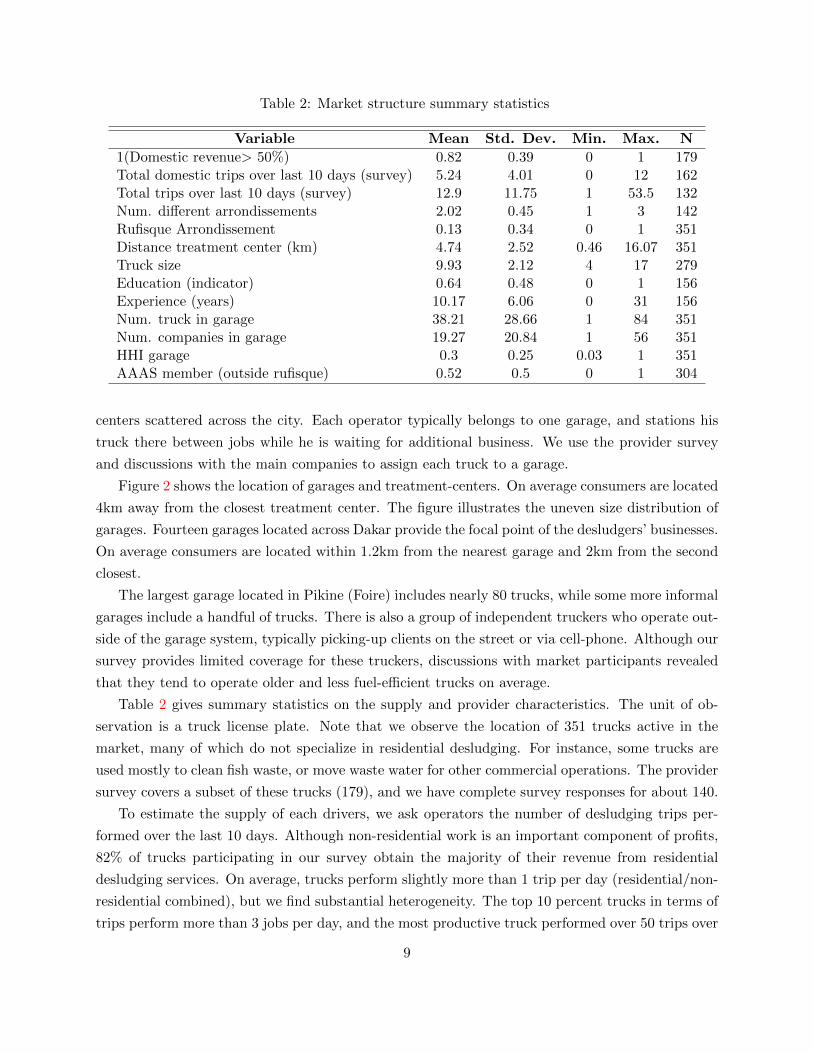
Table 2: Market structure summary statistics

Variable Mean Std. Dev. Min. Max. N

1(Domestic revenue> 50%) 0.82 0.39 0 1 179Total domestic trips over last 10 days (survey) 5.24 4.01 0 12 162Total trips over last 10 days (survey) 12.9 11.75 1 53.5 132Num. different arrondissements 2.02 0.45 1 3 142Rufisque Arrondissement 0.13 0.34 0 1 351Distance treatment center (km) 4.74 2.52 0.46 16.07 351Truck size 9.93 2.12 4 17 279Education (indicator) 0.64 0.48 0 1 156Experience (years) 10.17 6.06 0 31 156Num. truck in garage 38.21 28.66 1 84 351Num. companies in garage 19.27 20.84 1 56 351HHI garage 0.3 0.25 0.03 1 351AAAS member (outside rufisque) 0.52 0.5 0 1 304

centers scattered across the city. Each operator typically belongs to one garage, and stations his

truck there between jobs while he is waiting for additional business. We use the provider survey

and discussions with the main companies to assign each truck to a garage.

Figure 2 shows the location of garages and treatment-centers. On average consumers are located

4km away from the closest treatment center. The figure illustrates the uneven size distribution of

garages. Fourteen garages located across Dakar provide the focal point of the desludgers’ businesses.

On average consumers are located within 1.2km from the nearest garage and 2km from the second

closest.

The largest garage located in Pikine (Foire) includes nearly 80 trucks, while some more informal

garages include a handful of trucks. There is also a group of independent truckers who operate out-

side of the garage system, typically picking-up clients on the street or via cell-phone. Although our

survey provides limited coverage for these truckers, discussions with market participants revealed

that they tend to operate older and less fuel-efficient trucks on average.

Table 2 gives summary statistics on the supply and provider characteristics. The unit of ob-

servation is a truck license plate. Note that we observe the location of 351 trucks active in the

market, many of which do not specialize in residential desludging. For instance, some trucks are

used mostly to clean fish waste, or move waste water for other commercial operations. The provider

survey covers a subset of these trucks (179), and we have complete survey responses for about 140.

To estimate the supply of each drivers, we ask operators the number of desludging trips per-

formed over the last 10 days. Although non-residential work is an important component of profits,

82% of trucks participating in our survey obtain the majority of their revenue from residential

desludging services. On average, trucks perform slightly more than 1 trip per day (residential/non-

residential combined), but we find substantial heterogeneity. The top 10 percent trucks in terms of

trips perform more than 3 jobs per day, and the most productive truck performed over 50 trips over

9

a 10 day period. Based on this and discussions with provider, we estimate that a typical job takes

between 1 and 2 hours from start to finish. Most truckers therefore operate with excess capacity,

while a small fraction operate at full capacity. Eighty-five percent of desludging operators in the

baseline provider survey stated that they could find more jobs if they wanted to make more money.

The compensation of drivers limits the incentive of drivers to compete aggressively for clients.

92% are paid on salary, and about half of desludgers report paying a commission for jobs are

referred to them from the garage (≈ 3,000 CFA/day). A portion of these revenues is redistributed

to company owners in the form of revenue-sharing agreements. For instance, desludgers in the

largest garages report being paid by the parking lot on days when they do not find work. Similarly,

among desludgers paid on commission, approximately 50% receive some payment even on days on

which they do no desludgings.

Prices are determined via bilateral negotiation between clients and truck drivers. The bottom

half of Table 1 provides statistics on how consumers find truckers. Walk-in clients at a parking lot

are allocated on a first-come/first-serve basis, and drivers from the same garage dot not compete

the client. Alternatively, drivers can find business privately using their cell-phone, or find client on

the street (street hailing). Since households must repeatedly order the service (every 6 or 12 months

on average), 44% of matches are realized via referrals or repeat use (e.g. household members or

neighbors). Note that households do not sign long-term contracts with providers, and prices are

negotiated for each trip.

Price competition between garages is in part coordinated by a trade association (Association of

Desludging Operators, or AAAS). We estimate that 50% of trucks belong to a company in which at

least one truck has ties with AAAS, and 28% of drivers report being directly affiliated. Membership

is concentrated among multi-truck companies. The four largest companies in the market, which

operate about 20% of all trucks, are all involved in the management of AAAS.

The official role of the Association is to help operators to collaborate on the procurement of truck

parts, and distribute large, lucrative government/commercial contracts, which are awarded through

the Association. The influence of the Association likely extends beyond member companies, and

affects the provision of residential contracts throughout the city. This is because AAAS controls

the largest garages in the city (where non-member trucks can park), and distributes contracts

and services to member and non-member companies. The threat of being excluded represents large

profit losses; for instance associated with the loss of non-residential contract, and/or a more difficult

access to truck parts.

We have incomplete data on the cost of joining the association and/or being affiliated with

a garage. Our surveys reveal that operators typically pay a fee to join, but do not pay regular

dues. Fees for being associated with a garage vary widely, sometimes even within the same garage.

For instance, 66 and 86 percent of drivers belonging to the two largest garages, Foire and SICAP,

reported paying garage membership fees. Median reported monthly fees are 12,000 CFA per truck

(approximately $24). Desludgers who belong to SICAP also pay 1,000 CFA per job that they win

10

Figure 3: Spatial distribution of average prices and demand for mechanical desludging

(a) Average transaction prices (b) Transaction probabilities

through the parking lot.9

2.3 A first look at collusion

In this section, we compare prices and take-up rates for mechanical desludgings in areas of Dakar

controlled by the Association, with those in the Rufisque sub-market. Companies in this area

operate independently of AAAS. We use this analysis to provide an upper bound on the effect of

collusion in the market.

In the 1990s, a single company was providing desludging services in Rufisque (UPAMA); a

fish product processing company. This company was asked by the city administration to provide

affordable residential desludging to the growing population of Dakar. The company sets a price

of 15,000 CFA, to let the maximum number of individuals access this service. Over time, new

companies entered the market to serve a growing demand, and had to match UPAMA’s base price

in order to get business. To the best of our knowledge, UPAMA does not receive a subsidy to

provide the service at a low price, and this price reflects the cost of mechanical desludging in the

area. The proximity of the Rufisque treatment plant helps reduce the variable cost of the service

relative to other areas of Dakar. With a relatively small number of domestic desludging trucks in

Rufisque, people sometimes have to wait several days before having an available truck.

Figure 3 plots the (smoothed) distribution of prices and demand across those two different

neighborhoods. The boundaries of the competitive area are highlighted in yellow (south-east). The

median price in Rufisque is 15,000 CFA, compared to 25,000 CFA in the rest of the city (prices in

the figures are expressed in 10,000 CFA). Therefore, the Rufisque median price roughly corresponds

9These figures are from the end-line survey of desludging operators, which occurred in March 2015

11

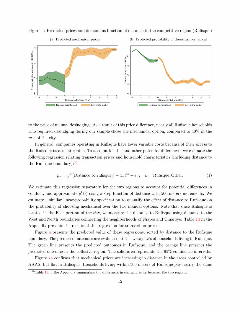
Figure 4: Predicted prices and demand as function of distance to the competitive region (Rufisque)

(a) Predicted mechanical prices

1015

2025

Aver

age

pric

e fo

r mec

hani

cal (

1,00

0 C

FA)

-3 -2 -1 0 1 2 3 4 5 6Distance to Rufisque (Km)

Rufisque neighborood Rest of the market

(b) Predicted probability of choosing mechanical

.5.6

.7.8

.91

Dem

and

for m

echa

nica

l (%

)

-3 -2 -1 0 1 2 3 4 5 6Distance to Rufisque (Km)

Rufisque neighborhood Rest of the market

to the price of manual desludging. As a result of this price difference, nearly all Rufisque households

who required desludging during our sample chose the mechanical option, compared to 40% in the

rest of the city.

In general, companies operating in Rufisque have lower variable costs because of their access to

the Rufisque treatment center. To account for this and other potential differences, we estimate the

following regression relating transaction prices and household characteristics (including distance to

the Rufisque boundary):10

pit = gk (Distance to rufisquei) + xitβk + εit, k = Rufisque,Other. (1)

We estimate this regression separately for the two regions to account for potential differences in

conduct, and approximate gk(·) using a step function of distance with 500 meters increments. We

estimate a similar linear-probability specification to quantify the effect of distance to Rufisque on

the probability of choosing mechanical over the two manual options. Note that since Rufisque is

located in the East portion of the city, we measure the distance to Rufisque using distance to the

West and North boundaries connecting the neighborhoods of Niayes and Thiaroye. Table 14 in the

Appendix presents the results of this regression for transaction prices.

Figure 4 presents the predicted value of these regressions, sorted by distance to the Rufisque

boundary. The predicted outcomes are evaluated at the average x’s of households living in Rufisque.

The green line presents the predicted outcomes in Rufisque, and the orange line presents the

predicted outcome in the collusive region. The solid area represents the 95% confidence intervals.

Figure 4a confirms that mechanical prices are increasing in distance in the areas controlled by

AAAS, but flat in Rufisque. Households living within 500 meters of Rufisque pay nearly the same

10Table 13 in the Appendix summarizes the differences in characteristics between the two regions.

12

price as their neighbors; roughly 15,000 CFA. The gap widens significantly as we move more than

1 Km away from the boundary. For distances greater than 1.5 Km, the average transaction prices

reach close to 25,000 CFA, and the price schedule is independent of distance to the competitive

region.

Figure 4b analyzes the effect of distance to Rufisque on the probability of choosing the mechan-

ical option (over both manual options). As before, this transaction probability is evaluated at the

mean characteristics of households in Rufisque, to eliminate any compositional effects. The effect of

distance on demand mimics the price results, suggesting that demand for mechanical desludging is

elastic. Households within one kilometer of the boundary are choosing using mechanical desludging

at a much higher rate than in the rest of the AAAS-controlled areas. The predicted probability in

and around Rufisque is estimated at roughly 95%, compared to about 60% in the rest of the city.

Note that this predicted fraction of users is larger than the unconditional probability reported in

Figure 3. This is because Rufisque households have an easier access to mechanical services (i.e.

predicted probability is evaluated at the average x of Rufisque households).

Figures 5a and 5b illustrate another important difference between the two areas: price dis-

persion. Since prices in Rufisque reflect desludging costs, we observe very limited dispersion in

transaction prices across households. In contrast, prices are very dispersed in areas controlled by

the association. Roughly 25% of households in this area pay prices that are comparable to the ones

paid in Rufisque. The remaining consumers pay prices that are much higher, and a sizable fraction

are pay more than double the Rufisque.

Importantly, Figure 5b shows that prices are dispersed across consumers even within narrowly

defined neighborhoods. The figure plots the distribution of a price residual obtained after expressing

prices relative to their neighborhood average (i.e. 27 zones). The inter-quartile range of residual

prices is 1,784 in Rufisque, compared to 8,570 in the rest of the market. In contrast, the IQR of

price levels is 10,000 CFA. This suggests that cost-related factors like accessibility and distance to

treatment center only explain a small fraction of the observed dispersion in prices paid by consumers

in the area controlled by the Association.

Finally, we use data on the number of trips per truck to measure the capacity utilization of

firms operating in both regions. Consistent with the demand results above, Figure 6 shows that the

distribution of the number of trips is very different between the two areas. Most trucks in Rufisque

perform between 25 and 40 trips per 10 days period, compared to less than 15 in the rest of the

market.

Table 3 presents differences in supply controlling for variables characterizing the trucker and

the garages they are affiliated with. Truckers in Rufisque perform on average 29 more trips over a

10 day horizon. This is despite the fact that the number of trucks per capita is larger in Rufisque

(see Table 13). Recall that the average number of trips in the full sample is 12.82. Truckers in

Rufisque are therefore used at nearly full capacity. Figure 6 illustrates this point by plotting the

distribution of trips across the two regions. The median truck in Rufisque performed 2.5 trips per

13

Figure 5: Distribution of mechanical prices in Rufisque and in the rest of Dakar

(a) Price levels

0.2

.4.6

.8Fr

actio

n

10 15 20 25 30 35 40 45 50 55 60Price (CFA/1000)

Rufisque Rest of Dakar

Note: Width = 5,000 CFA

(b) Price residuals

0.2

.4.6

Frac

tion

-20 -10 0 10 20 30 40Within neighborhood residual (CFA/1000)

Rufisque Rest of Dakar

Note: Width = 5,000 CFA

day during our survey period, compared to 1 trips per day in the rest of the market.

We observe the same increase in magnitude in the number of domestic trips. A larger fraction

of Rufisque trucks are doing mostly residential desludging, and perform on average 8.62 additional

domestic jobs over a 10 day horizon. Finally, Rufisque trucks are less likely to do business in

other neighborhoods than trucks in other regions. This is consistent with the price results around

the boundary: Rufisque trucks are unlikely to serve clients outside of their neighborhood due to

capacity constraints.

Note also that the AAAS dummy is imprecisely estimated, but positive across all specifications.

In other words, we do not find evidence that companies directly associated with the AAAS are less

productive than others operating in the same neighborhood; where productivity is measured as jobs

per truck. This is likely because trucks affiliated with the main garages tend to be better located,

and more likely to match with consumers. Independent truckers are forced to pick-up clients from

more isolated locations, or directly on the street.

In summary, this analysis suggests that there exists clear differences in competitive conduct

between areas that are controlled by the association and the Rufisque neighborhood. Assuming

that unobserved cost differences are continuously distributed around the Rufisque boundary, the

results establish that the average households in the association-controlled neighborhoods pay a

significantly higher markup on mechanical desludging price. This is consistent with the hypothesis

that the association is successful at restricting supply and maintaining high prices in most areas

of Dakar. One caveat to this interpretation is the possibility that companies operating in Rufisque

are not comparable to companies operating in the rest of the market, either because of their cost

structure or ownership. In the next section we use data on from the auction platform in order to

directly measure the extent to which firms behave competitively.

14

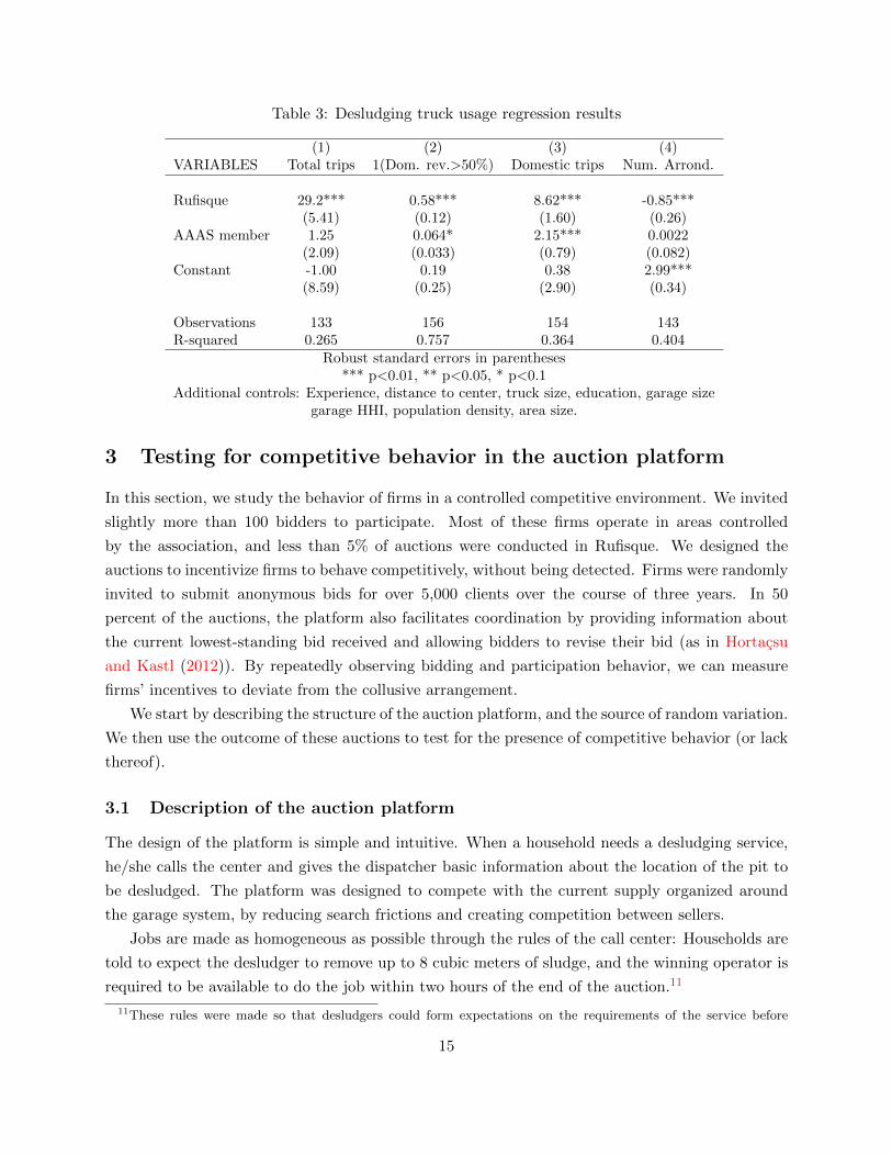
Table 3: Desludging truck usage regression results

(1) (2) (3) (4)VARIABLES Total trips 1(Dom. rev.>50%) Domestic trips Num. Arrond.

Rufisque 29.2*** 0.58*** 8.62*** -0.85***(5.41) (0.12) (1.60) (0.26)

AAAS member 1.25 0.064* 2.15*** 0.0022(2.09) (0.033) (0.79) (0.082)

Constant -1.00 0.19 0.38 2.99***(8.59) (0.25) (2.90) (0.34)

Observations 133 156 154 143R-squared 0.265 0.757 0.364 0.404

Robust standard errors in parentheses*** p<0.01, ** p<0.05, * p<0.1

Additional controls: Experience, distance to center, truck size, education, garage sizegarage HHI, population density, area size.

3 Testing for competitive behavior in the auction platform

In this section, we study the behavior of firms in a controlled competitive environment. We invited

slightly more than 100 bidders to participate. Most of these firms operate in areas controlled

by the association, and less than 5% of auctions were conducted in Rufisque. We designed the

auctions to incentivize firms to behave competitively, without being detected. Firms were randomly

invited to submit anonymous bids for over 5,000 clients over the course of three years. In 50

percent of the auctions, the platform also facilitates coordination by providing information about

the current lowest-standing bid received and allowing bidders to revise their bid (as in Hortacsu

and Kastl (2012)). By repeatedly observing bidding and participation behavior, we can measure

firms’ incentives to deviate from the collusive arrangement.

We start by describing the structure of the auction platform, and the source of random variation.

We then use the outcome of these auctions to test for the presence of competitive behavior (or lack

thereof).

3.1 Description of the auction platform

The design of the platform is simple and intuitive. When a household needs a desludging service,

he/she calls the center and gives the dispatcher basic information about the location of the pit to

be desludged. The platform was designed to compete with the current supply organized around

the garage system, by reducing search frictions and creating competition between sellers.

Jobs are made as homogeneous as possible through the rules of the call center: Households are

told to expect the desludger to remove up to 8 cubic meters of sludge, and the winning operator is

required to be available to do the job within two hours of the end of the auction.11

11These rules were made so that desludgers could form expectations on the requirements of the service before

15

Figure 6: Distribution of trips per trucks across arrondissements (last 10 days)

0.1

.2.3

.4Fr

actio

n

0 5 10 15 20 25 30 35 40 45 50 55

Avg. trips (other) Avg. trips (Rufisque)

The call center dispatcher sends the job out for bidding to 8-20 desludging operators via text

message. Both independent and affiliated operators are invited to bid on every job, and bidding is

done anonymously. The platform informs the bidder as to the number of operators who have been

invited and the number that are single truck operators versus those affiliated with larger companies,

but not the specific identities of the other bidders.

The timing of each auction proceeds as follows. The invited desludging operators have one hour

to bid on the job using text messages, and the operator with the lowest offer wins the job. In case

of a tie, the bidder who sent the earlier bid wins, encouraging prompt bidding. The dispatcher

then calls the household, informs them of the winning bid, and asks if the household accepts that

price. If the household accepts, the desludging operator is given the household-specific information,

and plans the remainder of the transaction directly with the household. Households pay desludgers

directly.12 The final winning bid is sent to all desludgers who have been invited to participate in

the auction, but not the identity of the winner.

There are three main layers of randomization in the auction platform: (1) the auction format,

(2) the number of bidders invited to the auction, and (3) the identities of the bidders invited to

submitting a bid. Desludgers with trucks less than 8 cubic meters are allowed to participate, but they must be readyto do more then one trip to empty a household’s tank. Similarly, desludgers with tanks larger than 8 cubic metersare not required to take more than 8 cubic meters when they perform the service.

12After the job has been completed, customers respond to customer satisfaction surveys conducted by phone inorder to ensure that quality of desludgings contracted through the call center remain high. In cases where thecustomer is dissatisfied or reports paying a price higher than the final auction bid, the job is investigated and thedesludger is penalized in terms of future invitations to auctions if they are found to be at fault.

16

the auction. We exploit this randomization in order to measure how the desludgers change their

bidding strategies across formats, and how competition and the identity of bidders affect auction

prices.

The auction format is randomized between a closed and revisable bidding format; each selected

with 50-50 probability. In the first, the “sealed-bid format”, bidders receive no updates after the

auction begins and have one hour to submit a single bid. Bidders in this format are not allowed to

change their bids after they have been submitted. In the second, the “revisable format”, bidders

are given updates about the standing low bid every 15 minutes and 5 minutes before the auction

closes, and can submit a new, lower bid any time. In both cases, desludgers receive text messages

reminding them that they have been invited to the auction at the same interval (every 15 minutes

and 10 minutes before the end of the auction).

Invitations are randomized between the 104 desludging operators in the system. The number of

invited bidders is uniformly distributed between 8 and 20. Invitation probabilities are independent

of the distance to the caller, but differ across bidders as a function of past participations. We

calculate the invitation probability as a piece-wise linear function of the number of valid bids

submit by a truckers in the prior months. This probability is truncated at the bottom and top to

ensure that the invitation probability is bounded away from zero, and less than 50%.

We ran 5162 auctions for desludging services through the call center in collaboration with the

Senegalese Office of Sanitation (ONAS) from July 2013 through April 2017. We drop auctions with

outlier bids (above 60,000), and auctions performed for subsidized households. The final sample

includes 4,485 auctions, including 3,700 with at least one bid. We made one change to the platform

in January 2015. At that time, the management of the platform was transferred to ONAS, and

the invitation rule was modified. In particular, rather than over-sampling “active” participants,

the probability of being invited became IID across truckers. Also, the number of invited bidders

decreased on average from 14 to 11. Although these two changes affected the performance of the

platform (less competition), it did not affect the random assignment of bidders to formats or clients.

Slightly more than half of auctions were performed prior to the design change (54%).

Figure 7 illustrates the distribution of auctions across the period of analysis. Starting in March

2014, the platform was heavily advertised across our target region, which led to an increase in the

number of calls per month. At the peek, the platform ran between 300 and 400 auctions per month.

The platform was much less advertised after the transfer to ONAS, and as a result the number

of callers dropped. The figure also highlights seasonalities in demand. The high-demand months

corresponds to the rainy season in Senegal.

Table 4 summarizes the number of auctions and participants before and after the platform

design change. The number of completed desludging is smaller than the number of callers. On

average the acceptance probability is about 30%. This is in part because the platform was not

designed to match clients with the most competitive set of potential bidders. The randomization

implies that clients often receive a small number of quotes, or are matched with distant truckers.

17

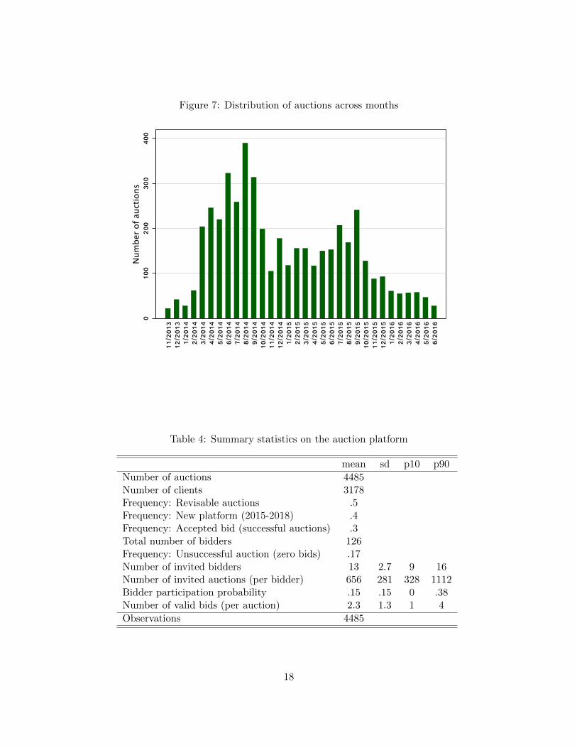
Figure 7: Distribution of auctions across months

010

020

030

040

0Num

ber

of auctions

11/2

013

12/2

013

1/20

142/

2014

3/20

144/

2014

5/20

146/

2014

7/20

148/

2014

9/20

1410

/201

411

/201

412

/201

41/

2015

2/20

153/

2015

4/20

155/

2015

6/20

157/

2015

8/20

159/

2015

10/2

015

11/2

015

12/2

015

1/20

162/

2016

3/20

164/

2016

5/20

166/

2016

Table 4: Summary statistics on the auction platform

mean sd p10 p90

Number of auctions 4485Number of clients 3178Frequency: Revisable auctions .5Frequency: New platform (2015-2018) .4Frequency: Accepted bid (successful auctions) .3Total number of bidders 126Frequency: Unsuccessful auction (zero bids) .17Number of invited bidders 13 2.7 9 16Number of invited auctions (per bidder) 656 281 328 1112Bidder participation probability .15 .15 0 .38Number of valid bids (per auction) 2.3 1.3 1 4

Observations 4485

18

Below we exploit this variation to identify demand for desludging at the platform.

The table also illustrates the experience and participation rate of bidders. On average, bidder

were invited to bid in 656 auctions. The participation rate is fairly low. The probability of

submitting a bid is about 15%, which leads to 2.3 valid bids per auction. This hides substantial

heterogeneity across bidders however, as we discuss below.

3.2 Hypothesis and identification strategy

We measure the stability of the cartel by identifying bidders behaving competitively in the auctions.

We do so by exploiting the random assignment of bidders to clients and auction formats to test the

null hypothesis of competitive bidding. Since each auction is anonymous and performed over a short

period of time, it is unlikely that bidders are able to organize a “strong” cartel ring to suppress

competition and select the lowest-cost firm. Instead, a rejection of this hypothesis is consistent

with tacit collusion.

To test this hypothesis, we first identify strategies that are inconsistent with competitive bidding

(e.g. Porter and Zona (1993), Porter and Zona (1999), Chassang et al. (2019)). An action is defined

as “collusive” if a bidder submits a non-meaningful bid in an effort to suppress competition among

cartel members (i.e. avoidance of competition). Conversely, we classify dominant strategies as

“competitive”, since they are associated with individual profit maximization. This identification

strategy relies on documenting the prevalence of strategies that are either dominated and dominant

for all bidders, irrespective of their cost. Since the platform randomizes the auction format, we

focus on identifying dominant/dominated actions that are specific to each strategic environment.

The first one focuses on the presence of identical bids (or ties) in sealed-bid first-price auctions.

Excessive correlation in bids is a common “red-flag” used by antitrust authorities.13 In our setting,

under the collusion interpretation, identical bids reflect a tacit agreement between firms to use

focal prices in certain neighborhoods. Targeting focal prices used in the residential market softens

competition by turning the auction into a lottery and allocating the good to participants who

submit early bids. This is a dominated strategy, since a bidder can do strictly better by bidding

below these focal prices, and increasing its probability of winning the auction.

In the revisable auction format, firms can avoid “tying” by submitting a bid that undercuts the

current lowest standing bid. As discussed in Haile and Tamer (2001), if a firm chooses to submit a

bid it must be that his/her cost is lower than the previously advertised “bid to beat”. In contrast

a firm can avoid competing by matching the current lowest bid, bidding above, or not bidding at

all.14 Conditional on submitting an offer after a prior bid was placed, matching or bidding above

the current lowest bid is analogous to submitting a non-serious bid. Note that this strategy can

13Since antitrust laws are not well enforced in Senegal, and the fear of being detected does not play an importantrole. Mund (1960) and Comanor and Schankerman (1976) provide early analysis of identical bids used in cartel cases,and McAfee and McMillan (1990) provide a theoretical discussion of the efficiency of this type of strategies.

14Not submitting a bid when the cost is lower than the current lowest bid is also a violation of profit maximization,but it is not testable without observing the private cost of each bidder.

19

still lead to a transaction, because some bidders are penalized after providing low service quality

in the past (penalty = 1,000 CFA). Rival bidders are only informed about the bid amount, and not

about the penalty status of rivals. Given this uncertainty, a competitive player should bid slightly

below to increase the probability of winning the contract.15

The timing of bidding and the probability of sending a revised bid also reveals information

about the competitiveness of a player. Bidding in the closed portion of the revisable auction is a

dominant strategy if firms are maximizing individual profits.16 Recall that unlike on eBay, sniping

in the platform only affects the information provided to other bidders, and not the probability that

a bid is rejected by the platform. Bidders have 10 minutes to submit a bid after the last message,

and the platform gives an additional 5 minutes “grace” period to ensure that all bids are received.

Since winning bidders pay their bid, it is optimal for firms to wait until the closed portion to submit

their bid. Doing so limits the likelihood that the bid is undercut. Also, if bidding is costly, firms

are better off learning about rival bids before bidding, rather than having to submit multiple offers

over the course of the auction. In contrast, submitting an early bid can be viewed as an effort to

coordinate prices by sending a signal to rivals.

This approach relies on identifying behavior that fails to maximize expected profit, and does

not identify the intensions of bidders when committing those mistakes. Errors can arise also for

other reasons than tacit collusion. For instance Hortacsu et al. (2019) identifies the importance

of bounded-rationality in electricity auctions, assuming competitive bidding. More generally, the

presence of tying and early bidding is consistent with the possibility that firms occasionally submit

non-serious bids; either because of bounded-rationality or due to market conditions (e.g. good

outside option or high opportunity cost of time). This is an important caveat that applies to our

approach, as well as much of the literature on testing for collusion.

To provide further evidence consistent with tacit collusion we leverage the panel dimension of

the data to assess the persistence in bidders’ propensity to behave competitively. Recall that we

see the same bidders being invited to a large number of auctions (nearly 600 on average). We use

this to measure the extent to which bidders that systematically choose dominated strategies in

one format, are doing so in the other format as well. Similarly, we identify “competitive types” as

bidders who have a high propensity to choose dominant strategies across both formats, by adjusting

their bidding strategy depending on the invitation. For instance, a negative correlation between the

propensity to tie in the sealed-bid auction and bidding late in the open auction is consistent with

the existence of a group of collusive bidders. A zero (or positive) correlation would be consistent

with non-serious bidding.

15This argument assumes that the density of cost is continuous along the real time. If costs are discrete, and abidder happens to face a cost exactly equal to the lowest-standing bid, matching is consistent with profit maximization.Given that bidder heterogeneity is most likely caused by capacity utilization and proximity to the client, it is morelikely that the underlying distribution is continuous.

16Sniping on eBay is typically interpreted as evidence of common-value. See Roth and Ockenfels (2002) and Bajariand Hortacsu (2003) for an analysis. This is unlikely to be the case in our context, since heterogeneity in cost isdriven mostly by idiosyncratic factors such as distance or future commitments.

20

3.3 Empirical analysis

Our detection strategy relies first on comparing auction outcomes across the two formats. Since

the format is randomly assigned, this leads to a simple treatment effect regression estimated using

auction-level observations:

yt = α1 (Revisablet) + xtβ + εt (2)

where t indexes an auction, and yt measures four different auction outcomes. We analyze the

effect of the auction format on five outcomes variables: (i) winning bid amount, (i) indicator for

winning bid is tied, (ii) indicator for winning bid is a round number (5,000 CFA increment), (iii)

indicator winning bid occurs in the last time interval, and (iv) timing of the first bid. We include

observed characteristics in the regression for efficiency reasons, and to analyze their impact on

auction outcomes. The results are unaffected by their inclusion, since the treatment assignment is

balanced on covariates.17

We start by analyzing the distribution of of winning bids and their arrival times. Figure 8

contrasts those two distributions using separate histograms for revisable and sealed-auctions. The

winning bid distribution closely resembles the negotiated price distribution displayed in Figure 1,

especially for bids coming from the sealed-bid format. The distribution exhibits clear mass points

at common focal prices used in the regular market: 20, 22, 25, 30 and 35. The same mass points

are present in the revisable format sample, but there are clear differences. Winning bidders in the

revisable format are much more likely to under-cut those focal prices by 1,000 CFA, which leads to

a higher density at 23, 24 and 29. This implies that cash-transaction frictions cannot fully explain

the use of focal prices. The distribution of bids clearly shows that there exists a group of bidders

willing to use a finer price grid to undercut the current lowest standing bid.

Figure 8b similarly suggests the existence of a group of competitive bidders. In the sealed-bid

auctions, roughly 30% of winning bids are placed in the first 5 minutes. Since the tie-breaking rule

favors early bidders, this is optimal for competitive and non-competitive types. In the revisable

auctions, the mass of “early” winning bids is reduced substantially, and the modal winning bid is

placed after the last message (i.e. minute 50). In between these two extremes, the distribution of

bid time reflects the nudges created by the new messages.18

The fact that the winning bid time distribution does not look like the eBay platform where

over 90% of bids are received in the last minute, but is instead a mixture of two distributions, is

consistent with the idea that there exists a group of bidders who are not behaving competitively.

17Balance test results are available upon request.18Note that the distribution of bid time appears continuous around the message time. This is because the initial

platform recorded arrival time with a slight error. This is not the case in the revised platform. In that sub-sample,we observe clear discontinuities around the message times. To classify bids “last minute bids”, we round the arrivaltime up by two minutes if the bid time was recorded two minutes or less before the last message. Figure 8b plotsthe distribution of winning bid time for auctions performed under the initial design (i.e. prior to 2015). The revisedformat changed slightly the timing of reminder messages, which would introduce additional noise in the graphs. Thebi-modality of the distribution persisted after the change.

21

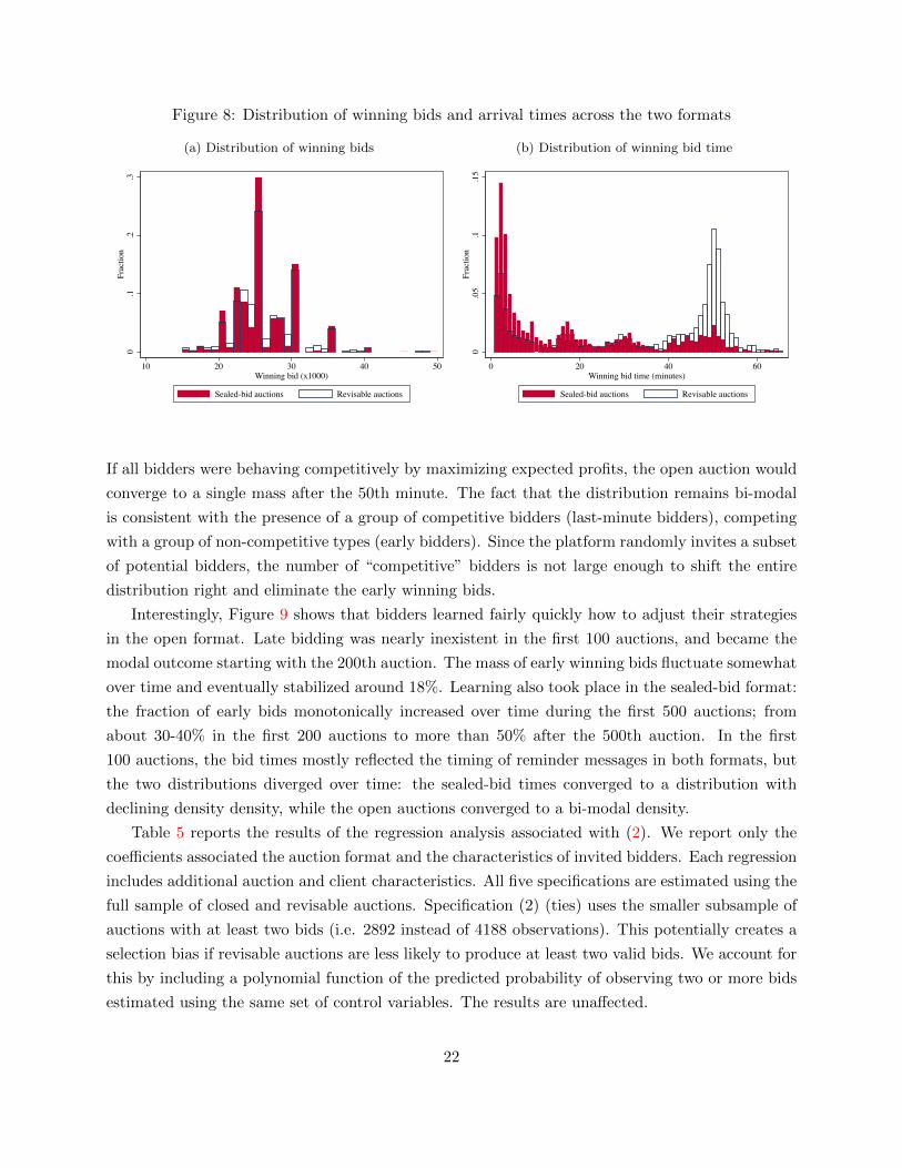
Figure 8: Distribution of winning bids and arrival times across the two formats

(a) Distribution of winning bids

0.1

.2.3

Frac

tion

10 20 30 40 50Winning bid (x1000)

Sealed-bid auctions Revisable auctions

(b) Distribution of winning bid time

0.0

5.1

.15

Frac

tion

0 20 40 60Winning bid time (minutes)

Sealed-bid auctions Revisable auctions

If all bidders were behaving competitively by maximizing expected profits, the open auction would

converge to a single mass after the 50th minute. The fact that the distribution remains bi-modal

is consistent with the presence of a group of competitive bidders (last-minute bidders), competing

with a group of non-competitive types (early bidders). Since the platform randomly invites a subset

of potential bidders, the number of “competitive” bidders is not large enough to shift the entire

distribution right and eliminate the early winning bids.

Interestingly, Figure 9 shows that bidders learned fairly quickly how to adjust their strategies

in the open format. Late bidding was nearly inexistent in the first 100 auctions, and became the

modal outcome starting with the 200th auction. The mass of early winning bids fluctuate somewhat

over time and eventually stabilized around 18%. Learning also took place in the sealed-bid format:

the fraction of early bids monotonically increased over time during the first 500 auctions; from

about 30-40% in the first 200 auctions to more than 50% after the 500th auction. In the first

100 auctions, the bid times mostly reflected the timing of reminder messages in both formats, but

the two distributions diverged over time: the sealed-bid times converged to a distribution with

declining density density, while the open auctions converged to a bi-modal density.

Table 5 reports the results of the regression analysis associated with (2). We report only the

coefficients associated the auction format and the characteristics of invited bidders. Each regression

includes additional auction and client characteristics. All five specifications are estimated using the

full sample of closed and revisable auctions. Specification (2) (ties) uses the smaller subsample of

auctions with at least two bids (i.e. 2892 instead of 4188 observations). This potentially creates a

selection bias if revisable auctions are less likely to produce at least two valid bids. We account for

this by including a polynomial function of the predicted probability of observing two or more bids

estimated using the same set of control variables. The results are unaffected.

22

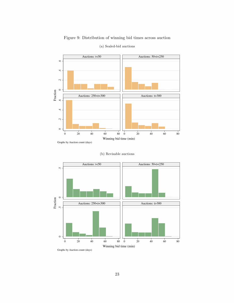
Figure 9: Distribution of winning bid times across auction

(a) Sealed-bid auctions

0.2

.4.6

0.2

.4.6

0 20 40 60 80 0 20 40 60 80

Auctions: t<50 Auctions: 50<t<250

Auctions: 250<t<300 Auctions: t>300

Frac

tion

Winning bid time (min)Graphs by Auction count (days)

(b) Revisable auctions

0.5

0.5

0 20 40 60 80 0 20 40 60 80

Auctions: t<50 Auctions: 50<t<250

Auctions: 250<t<300 Auctions: t>300

Frac

tion

Winning bid time (min)Graphs by Auction count (days)

23

Table 5: Effect of auction format on auction outcomes

(1) (2) (3) (4) (5)VARIABLES Winning bid 1(Ties) 1(Round) 1(Last message) First bid (min.)

1(Revisable) 0.101 -0.0892a -0.0927a 0.281a 3.216a

(0.112) (0.0156) (0.0162) (0.0141) (0.571)

Observations 3,627 2,501 3,627 3,627 3,627R-squared 0.353 0.054 0.082 0.145 0.220Mean dep. variable 25.73 0.191 0.526 0.279 17.17

Robust standard errors in parenthesesa p<0.01, b p<0.05, c p<0.1

The first column tests the equality of wining bids across the two formats. The point estimates

suggest that revisable auctions lead to offers that are on average 160 CFA larger than sealed-bid

auctions, but the difference is not statistically significant (p-value is about 12%).19 Although it is

interesting to learn about the effect of the format on average winning bids, from a theory perspective

there is no reason to believe that the two formats should be revenue equivalent (under collusion or

competition). This is because the revisable auction format has a “hard close”, and bids submitted

in the last 10 minutes are not observed by rivals. The revisable auction is best described as a

sequential auction: open followed by closed.

The next two specifications analyze the importance of ties and round bids. The probability that

the winning bidder ties in the sealed-bid auction is significantly higher (i.e. 9 percent). As column

(3) illustrates, this is explained by the fact that firms are significantly less likely to use round bids

in the open format. This is consistent with Figure 8a above. By revealing the current lowest bid at

the 50th minute, the revisable auction allows competitive bidders to submit bids that are “in the

money” relative to the standing low bid as of minute 50, and win the auction more often.

Importantly, the fraction of round bids and ties does not go to zero in the revisable format.

Table 15 in the Appendix presents the mean of each outcomes across the two formats. On average,

16.5% of revisable auctions end in a tie, compared to 25.6% for sealed. This is consistent the

presence of a group of non-competitive bidders, but is inconsistent with the hypothesis that biased

beliefs cause ties. It is likely that consumers do not have correct beliefs in the sealed-bid auction,

which could explain the presence of ties. This is less likely in the revisable format, since firms learn

quickly that failing to revise their bid down will result in a tie.

The last two specifications analyze the timing of bids. As Figure 8b suggested, winning bidders

in the revisable format are significantly more likely to submit a bid in the last 10 minutes of the

auction. The difference is 28 percentage points (i.e. 42% vs 14%). Similarly the first bid is received

earlier in the sealed-bid format (i.e. 19% vs 15.6%). The fact that the first bid arrives quickly

19In general, collusion is thought to be easier to sustain in open auctions environments (without hard close).See Robinson (1985), Graham and Marshall (1987), Marshall and Marx (2007), Athey, Levin, and Seira (2011) fortheoretical and empirical analysis of this in the context of english auctions.

24

on average in both formats explains the bimodal shape of the distribution of winning bid times.

Both estimates confirm that the auctions are composed of two groups of bidders: early bidders

in both formats (“non-competitive”), and bidders who submit late bids in the revisable format

(“competitive”).

Next, we investigate the correlation in bidding strategies across formats to provide support

for the collusion interpretation. Specifically, we test the hypothesis that bidders who avoid domi-

nated strategies behave competitively in both formats. To test this hypothesis we first construct

a “collusive-index” by estimating the probability that a bidder ties in the sealed-bid auction. We

estimate this probability by estimating the following Probit model:

Pr(Tieit|xit, θi) = Φ(−xitβ − θi) (3)

where θi is bidder i’s fixed-effect. This fixed-effect measures the bidder’s propensity to tie. We

interpret this variable as a continuous measure of the incentive of firms to deviate from the collusive

agreement. High θ bidders are less likely to deviate.

To reduce the measurement error in these θi, we focus on active bidders submitting at least 30

bids in the sealed-bid auctions. Since those bidders are participating at a much higher rate than the

average (30% compared to 10%), this sample includes the most experienced and attentive group of

bidders.20 40 bidders satisfy this criteria (out of roughly 109 participating bidders).

We estimate equation (3) using the sample of auctions with at least two valid bids. We control

for observed characteristics of the auction that affects the sample selection (e.g. time/neighborhood

fixed-effects, distance from garage and treatment center, aggregate time trends). We also control

for the experience of bidders to account for learning effects (i.e. number of auctions invited prior

to auction t).

Figure 10 illustrates the distribution of the collusion index across active bidders. The chi-

square statistic (169) clearly rejects the null hypothesis of equal fixed-effects, which confirms the

importance of bidder unobserved heterogeneity. To facilitate the interpretation, we normalized

the index by its standard-deviation. We also report results using a Bayesian Shrinkage correction

following the approach discussed in Chandra et al. (2016). This attenuates the importance of

measurement error.21 The sample includes a group of 11 bidders with a negative or close to zero

propensity to tie (more competitive types). The majority of bidders have a positive propensity

to tie (less competitive types). Fifteen bidders have an index above 1.5, and the remainders have

indices between 0.5 and 1.5.

Table 6 analyzes the correlation between bidders’ propensity to tie in the sealed-bid auction and

a set of firm and garage characteristics. The dependent variable is an indicator variable equal to one

for bidders in the top 2/3 of the distribution of θi. The first column controls for the membership

20The results are robust to varying the activity threshold from 20 to 40.21To implement this correction, we project the estimated fixed-effects on observed bidder characteristics: garage

FE, number of trucks, and truck size.

25

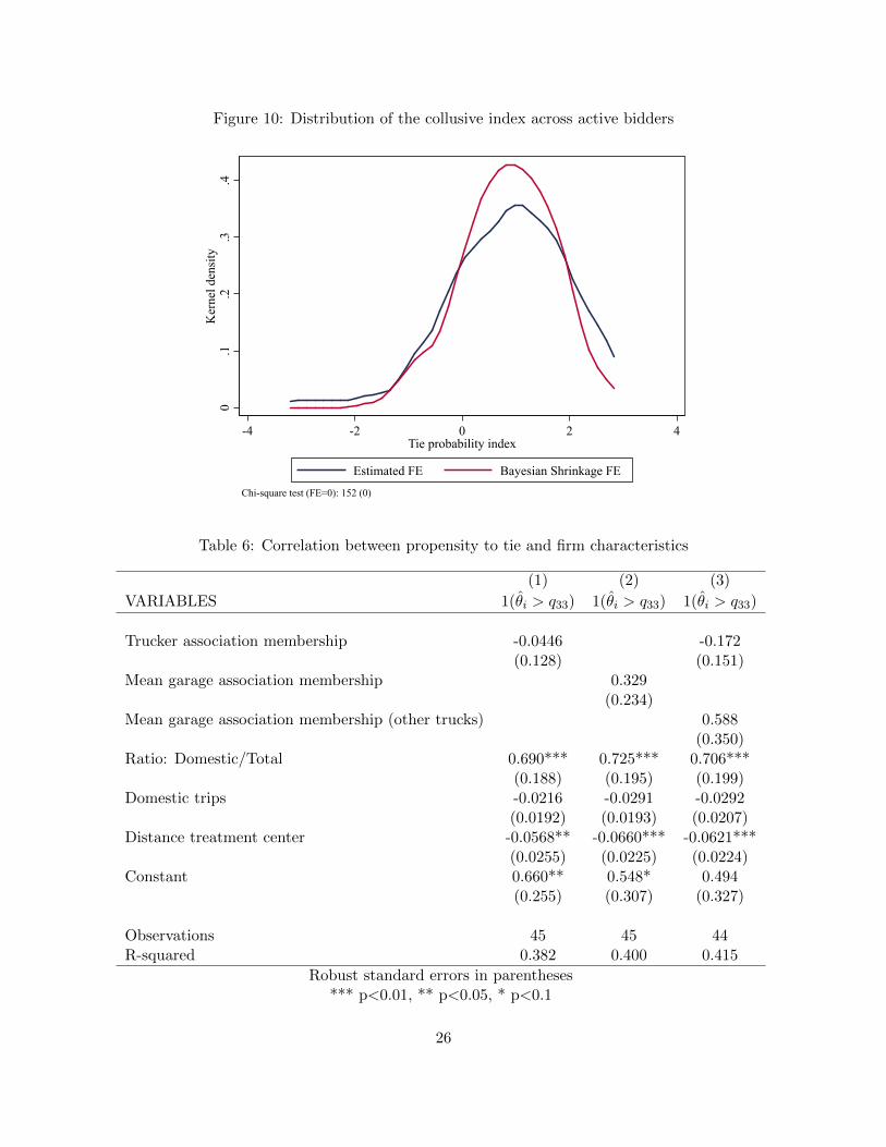
Figure 10: Distribution of the collusive index across active bidders

0.1

.2.3

.4K

erne

l den

sity

-4 -2 0 2 4Tie probability index

Estimated FE Bayesian Shrinkage FE

Chi-square test (FE=0): 152 (0)

Table 6: Correlation between propensity to tie and firm characteristics

(1) (2) (3)

VARIABLES 1(θi > q33) 1(θi > q33) 1(θi > q33)

Trucker association membership -0.0446 -0.172(0.128) (0.151)

Mean garage association membership 0.329(0.234)

Mean garage association membership (other trucks) 0.588(0.350)

Ratio: Domestic/Total 0.690*** 0.725*** 0.706***(0.188) (0.195) (0.199)

Domestic trips -0.0216 -0.0291 -0.0292(0.0192) (0.0193) (0.0207)

Distance treatment center -0.0568** -0.0660*** -0.0621***(0.0255) (0.0225) (0.0224)

Constant 0.660** 0.548* 0.494(0.255) (0.307) (0.327)

Observations 45 45 44R-squared 0.382 0.400 0.415

Robust standard errors in parentheses*** p<0.01, ** p<0.05, * p<0.1

26

of the truck to the association, and the second column controls for the association membership

among trucks belonging to the same garage. Both coefficients are positive, but the garage-level

variable has a stronger positive association with bidder’s propensity to tie. The last column shows

a similar effect, by controlling for both the own truck affiliation, and the average among other

garage members. This is consistent with the idea that garages play a role in monitoring deviations

and potentially punishment. The effect of “own” affiliation is theoretically

The next two variables control for the overall trucker’s output. On average, truckers that

perform more trips are more likely to bid competitively. However, truckers that rely more on

domestic desludging tend to bid less competitively. Finally, the distance between the garage and

treatment center is negatively associated with the propensity to tie. Bidders that are better located

in the market tend to behave less competitively in the auction.

To analyze the correlation between bidders’ collusive type and bidding strategies, we estimate

the following OLS regression estimated at the bid level:

yit = αθi + xitβ + εit (4)

where xit is a set of control variables describing the auction and the client. The parameter α

measures the correlation between the bidder collusive index (θ) and the choice variable y. We

consider five outcome variables controlled by the bidder: (i) bid amount in the sealed-bid auction,

(ii) indicator for round bid (5,000 increment), (iii) indicator for late bidding, (iv) indicator for bids

that are “out of the money”, and (v) time of first bid in the revisable auction.

Table 7 presents the main regression results using the shrinkage correction. Table 17 in the

Appendix presents the same specifications without the shrinkage correction. Standard errors are

clustered at the bidder level (40). Table 17a includes the results associated with bidding strategies

in the sealed-bid auctions. The first column shows that bidders with a high propensity to tie

are submitting significantly higher bids. The difference between competitive types (θ = −2) and

collusive types (θ = 2) is 4,400 CFA, or about 17% of the average bid placed. The second column

confirms that bidders who are more likely to tie, are also more likely to submit “focal” bids using a

grid with 5,000 CFA increments. However, all bidder types are equally (un)likely to submit a late

bid in the sealed-bid auction (column 3). This os consistent with the idea that both collusive and

competitive types have an incentive to bid early in the sealed auction due to the tie-breaking rule.

Table 17b shows similar results in the revisable auction sample. The first two columns analyze

the probability of submitting losing bids. To estimate this regression, we further restrict the sample

to bids placed after a price information message. Bidders who have a high propensity to tie in the

sealed-bid auction (high θ), are also more likely to submit a losing bid in the revisable auction.

Conditional on submitting a bid, those bidders are 9.3% less likely to undercut and 5.8% more

likely to bid above the current lowest standing bid. Since those bids were placed knowing the value

of the “bid to beat”, this result shows that bidders behaving non-competitively in the sealed-bid

27

Table 7: Relationship between bidders’ propensity to tie and bidding strategies (with shrinkagecorrection)

(a) Sealed-bid auctions

(1) (2) (3)VARIABLES Bid amount 1(Round bid) 1(Late bid)

Tie FE 1.11b 0.19a -0.049(0.51) (0.050) (0.066)

Observations 3,992 3,992 3,992R-squared 0.222 0.143 0.062Mean variable 27 0.60 0.21Nb active bidders 40 40 40

Clustered standard errors in parenthesesa p<0.01, b p<0.05, c p<0.1

(b) Revisable auctions

(1) (2) (3) (4)VARIABLES 1(Undercut) 1(Bid above) 1(Late bid) Bid time

Tie FE -0.093b 0.058b -0.27a -12.0a

(0.042) (0.024) (0.068) (2.75)

Observations 1,741 1,741 3,490 3,490R-squared 0.083 0.052 0.240 0.230Mean variable 0.37 0.043 0.21 26.7Nb active bidders 40 40 40 40

Clustered standard errors in parenthesesa p<0.01, b p<0.05, c p<0.1

The control variables include: time and arrondissement fixed-effects, distance from garage to client (1km bins),number of invited bidders, auction hour, morning and lunch time indicator, distance to treatment center, clientlat/long coordinates, population size, aggregate trend (cubic), new platform indicator, and experience of the bidder.

28

Figure 11: Distribution of participation frequencies across bidders

0.1

.2.3

Frac

tion

0 .2 .4 .6Participation frequencies

auction, are also more likely to avoid competition in the revisable auction.

The correlation between “tying” and “late bidding” is also negative. The point estimates

(−0.27) reveal that only bidders who have a low collusive index tend to submit bids after the last

message. The first bid placed by non-competitive bidders also arrive much earlier: the difference

between θ = −2 and θ = 2 is 48 minutes. This is in line with the idea that “collusive” types are

using their first bid as a signal to other collusive bidders invited to the auction.

One obvious way firms can suppress competition is by refusing to bid. Figure 11 presents

the distribution of participation frequencies across bidders. Indeed we observe that roughly 30% of

bidders never bid, and another 30% participate in in less than 20% of auctions they were invited to.

The group of active bidders represents the rest of the players; participation probabilities between

20 and 60 percent.

Table 8 analyses the relationship between bidders’ propensity to tie, and the decision to par-

ticipate in the auctions (Table 16 in the appendix presents the results without shrinkage). Recall

that we are only studying the participation decision of active bidders, and so it is reasonable to

expect that those bidders pay attention to the invitation message, and endogenously decide to enter

or not the auction. Columns (1)-(4) estimate a series of linear probability models accounting for

observed differences across auctions, and the collusive index. Each specification flexibly controls

for the distance between the bidder’s garage and the client. In specification (2) we interact θi with

an indicator variable equal to one if the client lives within 2 Km of the garage.

In columns (1) and (3), we see that non-competitive types are less likely to submit a bid,

29

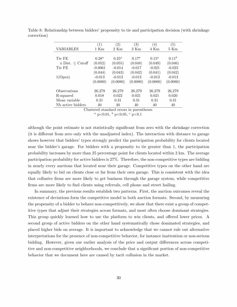
Table 8: Relationship between bidders’ propensity to tie and participation decision (with shrinkagecorrection)

(1) (2) (3) (4) (5)VARIABLES 1 Km 2 Km 3 Km 4 Km 5 Km

Tie FE 0.28a 0.25a 0.17a 0.15a 0.11b

x Dist. ≤ Cutoff (0.052) (0.055) (0.048) (0.049) (0.046)Tie FE -0.0061 -0.014 -0.017 -0.021 -0.023

(0.044) (0.043) (0.042) (0.041) (0.042)1(Open) -0.013 -0.013 -0.013 -0.013 -0.013

(0.0080) (0.0080) (0.0080) (0.0080) (0.0080)

Observations 26,279 26,279 26,279 26,279 26,279R-squared 0.018 0.022 0.021 0.021 0.020Mean variable 0.31 0.31 0.31 0.31 0.31Nb active bidders 40 40 40 40 40

Clustered standard errors in parenthesesa p<0.01, b p<0.05, c p<0.1

although the point estimate is not statistically significant from zero with the shrinkage correction

(it is different from zero only with the unadjusted index). The interaction with distance to garage

shows however that bidders’ types strongly predict the participation probability for clients located

near the bidder’s garage. For bidders with a propensity to tie greater than 1, the participation

probability increases by more than 25 percentage point for clients located within 2 km. The average

participation probability for active bidders is 27%. Therefore, the non-competitive types are bidding

in nearly every auctions that located near their garage. Competitive types on the other hand are

equally likely to bid on clients close or far from their own garage. This is consistent with the idea

that collusive firms are more likely to get business through the garage system, while competitive

firms are more likely to find clients using referrals, cell phone and street hailing.

In summary, the previous results establish two patterns. First, the auction outcomes reveal the

existence of deviations form the competitive model in both auction formats. Second, by measuring

the propensity of a bidder to behave non-competitively, we show that there exist a group of compet-

itive types that adjust their strategies across formats, and most often choose dominant strategies.

This group quickly learned how to use the platform to win clients, and offered lower prices. A

second group of active bidders on the other hand systematically chose dominated strategies, and

placed higher bids on average. It is important to acknowledge that we cannot rule out alternative

interpretations for the presence of non-competitive behavior, for instance inattention or non-serious

bidding. However, given our earlier analysis of the price and output differences across competi-

tive and non-competitive neighborhoods, we conclude that a significant portion of non-competitive

behavior that we document here are caused by tacit collusion in the market.

30

4 Measuring economic damages from collusion

In this section, we evaluate the economic damages of collusion in the market, by evaluating the

price and quantity effects of collusion. We do so by measuring the change in consumer surplus and

demand allowing all consumers to access more competitive prices.

We construct two counter-factual distributions that approximate more competitive environ-

ments. In the first one, we give consumers in the collusive neighborhoods access to the Rufisque

price distribution (competitive control). In the second scenario, we give all consumers access to

offers from auctions with competitive invitation lists (i.e. more competitive bidders and lower dis-

tance). This exercise is a partial equilibrium calculation of the effect of making the auctions more

competitive.

Demand mechanical desludging We use a discrete-choice model to measure demand and

willingness-to-pay. Let ri denotes the reservation price of consumer i, and pi denotes the best offer

that i receives for the mechanical service. Since consumers are choosing between mechanical and

one of two manual option (family or Baaypell), the reservation price is unobserved. Similarly, the

mechanical price offer is unobserved for consumers choosing the manual option.

This leads to an endogenous selection model. Following (Heckman, 1979), we parametrize the

distribution of reservation prices and offers as a bivariate normal distribution:(pi

ri

)=

(xiβ1

ziα+ xiβ0

)+

(ei1

ei0

)

where ei ∼ N(0,Σ), and zi is a variable that affects the mean reservation price, but does not

directly affect the mechanical price. Let σj denotes the standard-deviation of eij , and σ01 the

covariance between ei1 and ei0.

After receiving an offer pi, consumers choose the mechanical option if the surplus is positive:

yi = 1 If vi = ri − pi > 0→ ziα+ xi(β0 − β1) + ei0 − ei1 = ziα+ xiγ︸ ︷︷ ︸vi

+ui > 0 (5)

We estimate the model by MLE after normalizing σu = 1. Let α, γ, σ1 and ρu,e1 denote the

parameters corresponding to the surplus distribution in the collusive area.

To identify σ1 and ρu,e1 , we impose an exclusion restriction that the characteristics of household

i’s neighbors are uncorrelated with ei1. We construct our instrument in two steps. Fist, we estimate

by OLS the conditional mean of Baaypell prices in the city, using variables xi as regressors. Let

pb(x) denotes this predicted for a household with characteristic x. We then calculate the sample

average of pb(x) among other households living in the same block as household i; on average

there 4 households per block in our sample. This variable varies across households based on the

observed characteristics of i’s neighbors. The identifying assumption is that those attributes are

31

Table 9: Maximum likelihood estimates of the selection model

(1) (2)VARIABLES Mechanical Price Choice

Nbh. Baaybell price (avg) 0.147a

(0.0169)Nearest center (Km) 0.842a -0.149a

(0.117) (0.0154)Nearest garage (Km) 0.718a -0.148a

(0.236) (0.0300)Num. trucks (3km) 0.0289a -0.00558a

(0.00552) (0.000752)Wide road -0.236 -0.493a

(0.677) (0.0689)Tube meters 0.0512a -0.00540a

(0.0198) (0.00134)Number of rooms 0.148a 0.0287a

(0.0570) (0.00743)1(Own Refrigerator) 1.132a 0.245a

(0.321) (0.0395)ρu,e1 -0.270a

(0.0444)Observations 6,647 6,647

Robust standard errors in parenthesesa p<0.01, b p<0.05, c p<0.1

Controls: Arrondissement and month/year FEs,additional household characteristics (see Table 13)

independent of the distribution of mechanical price offers that household i receives (conditional on

its own characteristics xi), and are correlated with the reserve price ri.

Table 9 reports the estimation results. The specification includes additional of household and

neighborhood characteristics (see Table 13 for a detailed list). The model is estimated in the

sample of household living more than 1 km away from the Rufisque boundary. As before the

table highlights the role of distance to garages and treatment centers in determining prices and

demand. The average price of Baaypell (manual) is a strong predictor of the mechanical choice,

confirming that the two services are substitutes. The bottom two rows report correlation between

ui and ei1, as well as the inverse-mills ratio coefficient. We can easily reject the null hypothesis of

no endogenous selection. The correlation coefficient (ρu,e1 = −0.27) suggest that consumers who

receive high-price offers have low net surplus (i.e. high reservation price), consistent with models

of price discrimination.

Counterfactual price distributions To calculate the effect of making the price distribution more

32

competitive, we assume that the counter-factual offers are normally distributed with a different

means and variances. Let βcomp and σcomp1 denote the new location and spread parameters. We

use the superscript “obs” to indicate parameters that the reflect the observed market equilibrium.

We use two counter-factual distributions to measure the effect of collusion on demand for

mechanical desludging. The first one assumes that consumers in the collusive area have access

to the Rufisque price distribution (conditional on xi). Since there is essentially no endogenous

selection in that market (i.e. take-up is nearly 100%), we estimate this price distribution via OLS.

See specification (2) in Table 14 (Appendix) for the results. Let pcompi = xiβ

comp1 denotes the mean

offer that a consumer i living outside of Rufisque would receive in this counter-factual environment.

We use σcomp1 as an estimate of the standard-deviation of ei,1 in the competitive environment.

We obtain the second counter-factual distribution using the results of the auctions. In particular,

we estimate by OLS the mean and variance of the winning bid distribution, conditional on observed

characteristics of the client, and measures of competition in the auction. To control the invitation

list, we use the number of invited bidders, as well as the distance from the client to nearest invited

bidders’ garage. We measure both variables using the full list of invited bidders, as well as the list

of active bidders invited. To account for the presence of competitive and collusive types, we also

control for the number of bidders with difference levels of the collusive index (i.e. propensity to

tie). We use five equally spaced groups.

Table 10 presents the results of this regression. The number and distance to nearest garage

variables are strong predictors of the winning bid. Column (2) shows that controlling for the

number of competitive and collusive types helps explain differences in bids across auctions. Adding

one “very” competitive bidder to the auction leads to a 1,000 reduction in the winning bid. The

marginal effect is monotonically increasing in the collusiveness of the group. The marginal effect

of inviting more bidders in the top two groups actually leads to higher offers for consumers.

To construct a “competitive” auction, we construct an invitation list in which all competitive

types are invited (i.e. 12 active bidders in the first three groups). We set the minimum distance to

500 meters, and set the total number of invited bidders to 20 (maximum). Table 11 summarizes

the results of this exercise among all auctions that were conducted. Using this competitive bidder

list would lead to a reduction of 5,290 CFA in the average winning bid.

We aggregate these predicted auction prices at the neighborhood level. Let pcompi denotes the

mean of the offer distribution for all households in the survey. Since we observe limited character-

istics of the platform clients, we assume that the mean of the distribution of offers is common to

all households within a neighborhood. The variance of the residual of the winning bid regression

similarly gives us an estimate of σcomp1 . Note that there is no truncation in this sample, since we

observe both accepted and rejected offers.

Counterfactual demand and consumer-surplus We use the two competitive price distribu-

tions to predict the take-up rate of households in the survey. To construct this counter-factual,

33

Table 10: Effect of competition and collusion on winning bids

(1) (2) (3) (4)VARIABLES Bid Bid Bid (log) Bid (log)

# bidders: Very competitive -0.96a -0.040a

(0.13) (0.0050)# bidders: Competitive -0.35a -0.014a

(0.10) (0.0039)# bidders: Mildly competitive -0.077 -0.0023

(0.053) (0.0020)# bidders: Somewhat collusive 0.031 0.0020

(0.055) (0.0021)# bidders: Very collusive 0.083 0.0039c

(0.054) (0.0020)Min distance (Km) 0.063 0.060 0.0023 0.0021

(0.048) (0.048) (0.0018) (0.0018)Nb. Bidders -0.097a -0.068c -0.0033a -0.0024c

(0.031) (0.035) (0.0012) (0.0013)Active bidders x Less 10KM -0.21a -0.23a -0.0093a -0.011a

(0.040) (0.045) (0.0016) (0.0017)Min. distance (active) 0.094a 0.10a 0.0036a 0.0039a

(0.030) (0.029) (0.0011) (0.0011)1(Open) 0.13 0.10 0.0053 0.0044

(0.11) (0.11) (0.0043) (0.0043)

R-squared 0.313 0.325 0.327 0.342Competition effect (sd) 0.77 0.99 0.031 0.040

Robust standard errors in parenthesesa p<0.01, b p<0.05, c p<0.1

Table 11: Change in the winning bid distribution and acceptance probability from increasingcompetition within all auctions

mean sd p25 p50 p75

Price difference -5.29 1.00 -5.92 -5.26 -4.61Accept prob. (observed) 0.29 0.12 0.21 0.28 0.35Accept prob. (competition) 0.48 0.14 0.40 0.48 0.56∆ Accept prob. (%) 0.81 0.55 0.47 0.69 1.01

Observations 3626

34

we need to obtain an estimate of σobsu (normalized to 1 in the estimation). Recall that the uncon-

ditional mean of vi is the average difference between the reserve price ri and mechanical price pi.

Assuming that distance to the nearest treatment center (mechanical cost shifter) does not affect

the manual price, the effect of distance on participation identifies the scale of u:

γdist = β1,dist/σu → σobsu =

βobs1,dist

γobsdist

.

We use this calculate the mean and variance of the reserve price using the following two identities:

ri = σobsu · (ziα+ xiγ)︸ ︷︷ ︸

vobsi

+xiβobs1 and σobs

u =

√σ2

0 − 2σobs01 + σobs

12.

We assume that (ri, σ0) are invariant to the change in competition. This is justified by our assump-

tion that the manual service is competitively provided.

Putting these pieces together, we can calculate the distribution of consumer surplus in the

counter-factual environment as follows:

vcompi ∼ N

(ri − pcomp

i , σcompu

2).

The expected take-up probability and surplus for consumer i in the competitive environment can

be written as:

scompi = Pr(vcomp

i > 0) = 1− Φ(−(ri − pcompi )/σcomp

u ) (6)

E(vi) = scomp ×(ri − pcomp

i + σcompu

φ(−(ri − pcompi )/σcomp

u )

1− Φ(−(ri − pcompi )/σcomp

u )

)(7)

Table 12 reports the results of the two counterfactual experiments. Both scenarios lead to

sizable decrease in prices. Not surprisingly, the Rufisque price distribution yields the larges price

decline (i.e. 42% compared to 17% from the auction). This translates into large reduction in

residual price dispersion, and increase in consumer surplus. The Rufisque experiment increase the

average surplus fivefold, while the surplus increase from the auction corresponds to 160% of the

baseline allocation.

Finally, the bottom row shows the effect of collusion on the takeup probability. If consumers in

the collusive region had access to the Rufisque price distribution, the average takeup probability

would increase from 42% to 71%. This new equilibrium would still be lower than in Rufisque,

mostly because the area is more geographically dispersed, and some consumers do not have an

easy access to mechanical desludging (i.e. narrow streets or distant from treatment centers). The

increase in takeup from the auction is also large. The fraction of households choosing mechanical

desludging increases to 54%. Importantly, this is a lower bound on the effect of removing collusion

35

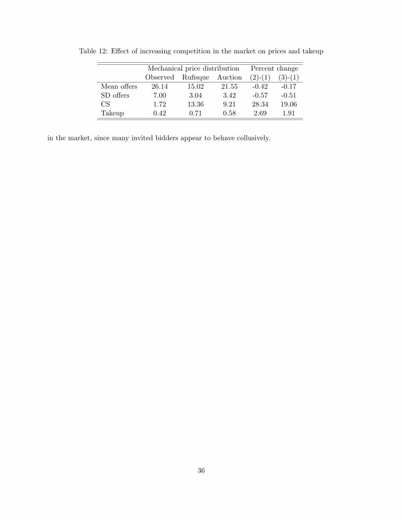
Table 12: Effect of increasing competition in the market on prices and takeup

Mechanical price distribution Percent changeObserved Rufisque Auction (2)-(1) (3)-(1)

Mean offers 26.14 15.02 21.55 -0.42 -0.17SD offers 7.00 3.04 3.42 -0.57 -0.51CS 1.72 13.36 9.21 28.34 19.06Takeup 0.42 0.71 0.58 2.69 1.91

in the market, since many invited bidders appear to behave collusively.

36

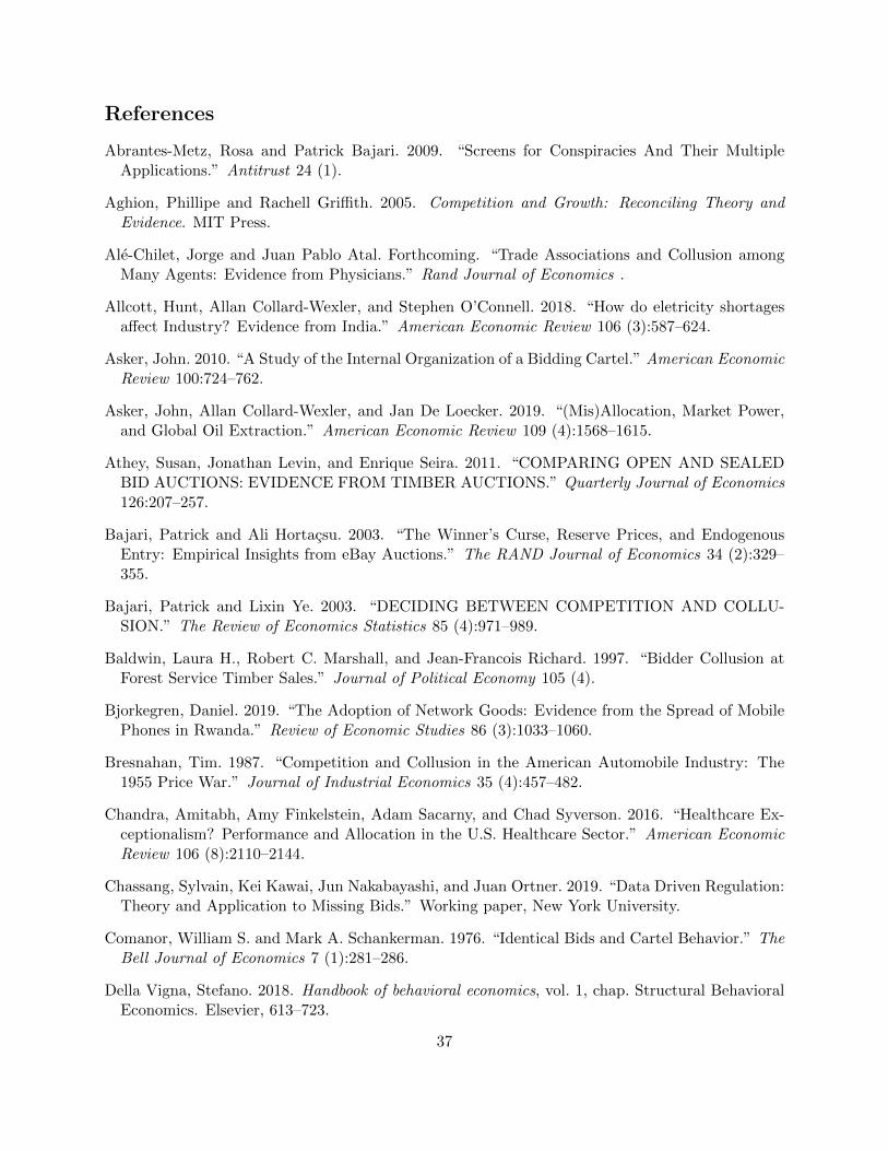
References

Abrantes-Metz, Rosa and Patrick Bajari. 2009. “Screens for Conspiracies And Their MultipleApplications.” Antitrust 24 (1).

Aghion, Phillipe and Rachell Griffith. 2005. Competition and Growth: Reconciling Theory andEvidence. MIT Press.

Ale-Chilet, Jorge and Juan Pablo Atal. Forthcoming. “Trade Associations and Collusion amongMany Agents: Evidence from Physicians.” Rand Journal of Economics .

Allcott, Hunt, Allan Collard-Wexler, and Stephen O’Connell. 2018. “How do eletricity shortagesaffect Industry? Evidence from India.” American Economic Review 106 (3):587–624.

Asker, John. 2010. “A Study of the Internal Organization of a Bidding Cartel.” American EconomicReview 100:724–762.

Asker, John, Allan Collard-Wexler, and Jan De Loecker. 2019. “(Mis)Allocation, Market Power,and Global Oil Extraction.” American Economic Review 109 (4):1568–1615.

Athey, Susan, Jonathan Levin, and Enrique Seira. 2011. “COMPARING OPEN AND SEALEDBID AUCTIONS: EVIDENCE FROM TIMBER AUCTIONS.” Quarterly Journal of Economics126:207–257.

Bajari, Patrick and Ali Hortacsu. 2003. “The Winner’s Curse, Reserve Prices, and EndogenousEntry: Empirical Insights from eBay Auctions.” The RAND Journal of Economics 34 (2):329–355.

Bajari, Patrick and Lixin Ye. 2003. “DECIDING BETWEEN COMPETITION AND COLLU-SION.” The Review of Economics Statistics 85 (4):971–989.

Baldwin, Laura H., Robert C. Marshall, and Jean-Francois Richard. 1997. “Bidder Collusion atForest Service Timber Sales.” Journal of Political Economy 105 (4).

Bjorkegren, Daniel. 2019. “The Adoption of Network Goods: Evidence from the Spread of MobilePhones in Rwanda.” Review of Economic Studies 86 (3):1033–1060.

Bresnahan, Tim. 1987. “Competition and Collusion in the American Automobile Industry: The1955 Price War.” Journal of Industrial Economics 35 (4):457–482.

Chandra, Amitabh, Amy Finkelstein, Adam Sacarny, and Chad Syverson. 2016. “Healthcare Ex-ceptionalism? Performance and Allocation in the U.S. Healthcare Sector.” American EconomicReview 106 (8):2110–2144.

Chassang, Sylvain, Kei Kawai, Jun Nakabayashi, and Juan Ortner. 2019. “Data Driven Regulation:Theory and Application to Missing Bids.” Working paper, New York University.

Comanor, William S. and Mark A. Schankerman. 1976. “Identical Bids and Cartel Behavior.” TheBell Journal of Economics 7 (1):281–286.

Della Vigna, Stefano. 2018. Handbook of behavioral economics, vol. 1, chap. Structural BehavioralEconomics. Elsevier, 613–723.

37

Deutschman, Josh, Jared Gars, Shoshana Griffith, Jean-Francois Houde, Terence Johnson, MollyLipscomb, Mbaye Mbeguere, Laura Schechter, and S. Zhu. 2016. “Using Market Mechanisms toIncrease the Take-up of Improved Sanitation.” Working Paper .

Doraszelski, Ulrich, Gregory Lewis, and Ariel Pakes. 2018. “Just Starting Out: Learning andEquilibrium in a New Market.” American Economic Review 108 (3):565–615.

Falcao Bergquist, Lauren and Michael Dinerstein. 2019. “Competition and Entry in AgriculturalMarkets: Experimental Evidence from Kenya.” Working paper, University of Michigan.

Graham, Daniel A. and Robert C. Marshall. 1987. “Collusive Bidder Behavior at Single-ObjectSecond-Price and English Auctions.” Journal of Political Economy 95 (6):1217–1239.

Haile, Philip A. and Elie Tamer. 2001. “Inference with an Incomplete Model of English Auctions.”Journal of Political Economy 111 (1).

Heckman, James. 1979. “Sample Selection Bias as a Specification Error.” Econometrica 47:153–161.

Hendricks, Kenneth and Robert H. Porter. 1989. “Collusion in Auction.” Annales d’economie etde statistique 15/16.

Hortacsu, Ali and Jakub Kastl. 2012. “Valuing Dealers’ Informational Advantage: A Study ofCanadian Treasury Auctions.” Econometrica 80 (6):2511–2542.

Hortacsu, Ali, Fernando Luco, Steven L. Puller, and Dongni Zhu. 2019. “Does Strategic Ability Af-fect Efficiency? Evidence from Electricity Markets.” American Economic Review 109 (12):4302–42.

Houde, Jean-Francois, Terrence Johnson, Molly Lipscomb, and Laura Schechter. 2020. “SustainableIntermediation: Using Market Design to Improve the Provision of Sanitation.” Working paper,University of Wisconsin-Madison.

Johnson, Terrence and Molly Lipscomb. 2020. “Pricing People into the Market: Targeting throughMechanism Design.” Working paper, University of Virginia.

Keniston, Daniel. 2011. “Bargaining and Welfare: A Dynamic Structural Analysis.” Workingpaper, Louisiana State University.

Marshall, Robert C. and Leslie Marx. 2007. “Bidder collusion.” Journal of Economic Theory133:374 – 402.

McAfee, Preston and John McMillan. 1990. “Bidding Rings.” American Economic Review82 (3):579–599.

Mund, Vernon A. 1960. “Identical Bid Prices.” Journal of Political Economy 68.

Organization, World Health and the United Nations Children’s Fund. 2017. “Progress on DrinkingWater, Sanitation and Hygiene: 2017 Update and SDG Baselines.” .

Plummer, Janelle and Piers Cross. 2006. “Delivering Sanitation to the Urban Poor: A ScopingStudy.” WSP Working Paper .

38

Porter, Robert H. 2005. “Detecting Collusion.” Review of Industrial Organization 26:147–167.

Porter, Robert H. and Douglas Zona. 1993. “Detection of bid rigging in procurement auctions.”Journal of Political Economy :518–538.

———. 1999. “Ohio School Milk Markets: An Analysis of Bidding.” The RAND Journal ofEconomics 30 (2):263–288.

Robinson, Marc S. 1985. “Collusion and the Choice of Auction.” The RAND Journal of Economics16 (1):141–145.

Roth, Alvin E. and Axel Ockenfels. 2002. “Last-Minute Bidding and the Rules for Ending Second-Price Auctions: Evidence from eBay and Amazon Auctions on the Internet.” American EconomicReview .

Ryan, Nicholas. Forthcoming. “The Competitive Effects of Transmission Infrastructure in theIndian Electricity Market.” American Economic Journal: Microeconomics .

39

Table 13: Mean differences in characteristics across neighborhoods

Others Rufisque Difference P-Value

Nearest center (Km) 4.55 2.84 1.71 0Nearest garage (Km) 1.23 1 .23 0Num. trucks (3km) 50.11 28.91 21.2 0Shopping: Street .11 .12 -.01 .594Shopping: Phone .18 .22 -.04 .056Wide road .12 .05 .07 0Tube meters 15.97 14.74 1.23 .15Concrete, no storage .65 .75 -.1 0Concrete, storage .32 .22 .09 0Slate roof .34 .23 .11 0Tile floor .41 .54 -.13 0Number of rooms 7.27 7.35 -.08 .6981(Multi HH) .24 .17 .07 .002Num. other HH 1.08 .75 .33 .003Household size 11.69 11.78 -.09 .805Adult share .67 .66 .01 .205Children share .33 .34 -.01 .305Women share .34 .34 0 .893Room used (%) .77 .79 -.02 .2981(Own Motorcycle) .08 .06 .01 .2941(Own Fan) .8 .85 -.05 .011(Own Refrigerator) .51 .57 -.06 .0141(Own Car) .16 .18 -.03 .182Own house .78 .87 -.09 0Num. earners 3.57 3.27 .31 .019Num. other earners .48 .54 -.06 .2721(Other earners) .27 .27 0 .887Adult earners (%) .51 .5 .02 .271

Table 14: Mechanical price regression across neighborhoods

(1) (2)VARIABLES Rest of the market Rufisque

Shopping: Street -1.15*** 0.76(0.42) (0.57)

Shopping: Phone -0.54* -0.47(0.32) (0.42)

Nearest center (Km) 1.25*** -2.17(0.25) (1.35)

Nearest garage (Km) 0.50** 1.26(0.22) (1.03)

Num. trucks (3km) 0.020*** 0.0048(0.0078) (0.051)

40

Wide road -1.16* 1.50(0.67) (1.07)

Tube meters 0.045*** 0.027(0.014) (0.022)

Concrete, no storage -1.64** 0.12(0.71) (1.17)

Concrete, storage -1.32* 1.30(0.72) (1.26)

Slate roof -1.51*** -0.31(0.41) (0.47)

Tile floor 1.67*** -0.15(0.31) (0.42)

Number of rooms 0.16*** -0.045(0.050) (0.057)

1(Multi HH) -0.22 -0.073(0.51) (0.90)

Num. other HH 0.26*** 0.33(0.095) (0.24)

Household size 0.068** 0.15***(0.029) (0.058)

Adult share 4.20 14.1(6.22) (9.83)

Children share 0.93 11.5(6.17) (9.28)

Women share -0.59 -0.85(0.82) (1.48)

Room used (%) 0.58 -0.60(0.76) (1.03)

1(Own Motorcycle) -0.18 -1.15(0.46) (0.72)

1(Own Fan) 0.24 0.31(0.40) (0.53)

1(Own Refrigerator) 1.36*** 0.097(0.31) (0.40)

1(Own Car) 0.42 0.69(0.32) (0.48)

Own house -0.28 0.0049(0.35) (0.56)

Num. earners -0.25** -0.43**(0.097) (0.20)

Num. other earners -0.10 -0.054(0.18) (0.19)

1(Other earners) -0.28 -0.41(0.43) (0.53)

Adult earners (%) 0.65 1.62(0.72) (1.31)

Constant 15.2** 5.95(6.43) (10.4)

Observations 2,941 350R-squared 0.197 0.179H0: Boundary coefficient (p-value) 0 0.24

41

H0: Common slopes (Chow) 0Standard errors in parentheses

*** p<0.01, ** p<0.05, * p<0.1

42

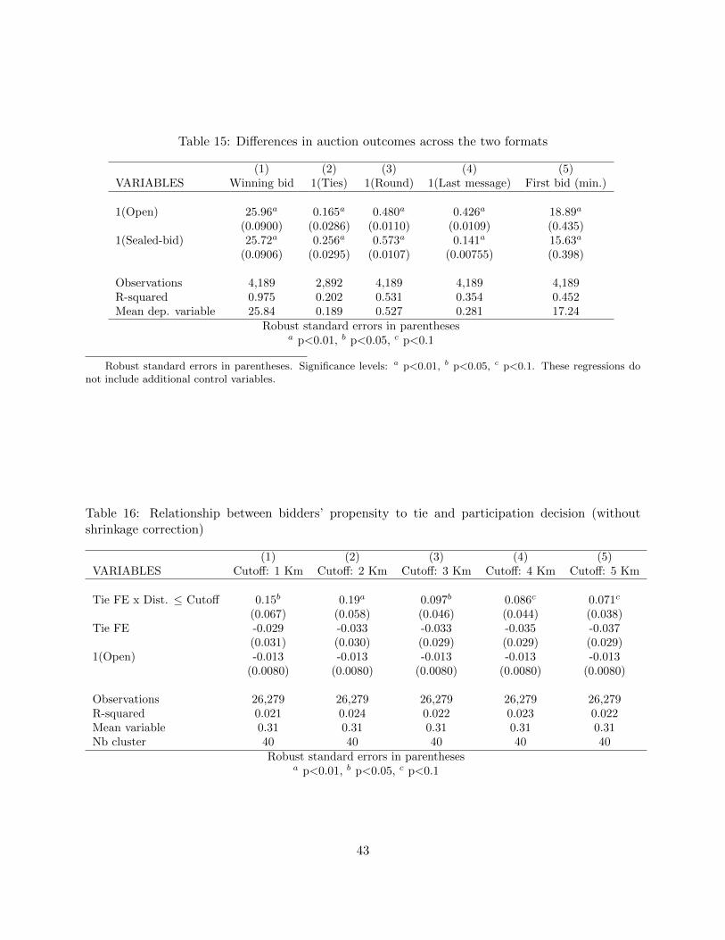
Table 15: Differences in auction outcomes across the two formats

(1) (2) (3) (4) (5)VARIABLES Winning bid 1(Ties) 1(Round) 1(Last message) First bid (min.)

1(Open) 25.96a 0.165a 0.480a 0.426a 18.89a

(0.0900) (0.0286) (0.0110) (0.0109) (0.435)1(Sealed-bid) 25.72a 0.256a 0.573a 0.141a 15.63a

(0.0906) (0.0295) (0.0107) (0.00755) (0.398)

Observations 4,189 2,892 4,189 4,189 4,189R-squared 0.975 0.202 0.531 0.354 0.452Mean dep. variable 25.84 0.189 0.527 0.281 17.24

Robust standard errors in parenthesesa p<0.01, b p<0.05, c p<0.1

Robust standard errors in parentheses. Significance levels: a p<0.01, b p<0.05, c p<0.1. These regressions donot include additional control variables.

Table 16: Relationship between bidders’ propensity to tie and participation decision (withoutshrinkage correction)

(1) (2) (3) (4) (5)VARIABLES Cutoff: 1 Km Cutoff: 2 Km Cutoff: 3 Km Cutoff: 4 Km Cutoff: 5 Km

Tie FE x Dist. ≤ Cutoff 0.15b 0.19a 0.097b 0.086c 0.071c

(0.067) (0.058) (0.046) (0.044) (0.038)Tie FE -0.029 -0.033 -0.033 -0.035 -0.037

(0.031) (0.030) (0.029) (0.029) (0.029)1(Open) -0.013 -0.013 -0.013 -0.013 -0.013

(0.0080) (0.0080) (0.0080) (0.0080) (0.0080)

Observations 26,279 26,279 26,279 26,279 26,279R-squared 0.021 0.024 0.022 0.023 0.022Mean variable 0.31 0.31 0.31 0.31 0.31Nb cluster 40 40 40 40 40

Robust standard errors in parenthesesa p<0.01, b p<0.05, c p<0.1

43

Table 17: Relationship between bidders’ propensity to tie and bidding strategies (without shrinkagecorrection)

(a) Sealed-bid auctions

(1) (2) (3)VARIABLES Bid amount 1(Round bid) 1(Late bid)

Tie FE 0.88a 0.13a 0.0025(0.18) (0.0097) (0.031)

Observations 3,992 3,992 3,992R-squared 0.245 0.170 0.054Mean variable 27 0.60 0.21Nb cluster 40 40 40

Robust standard errors in parenthesesa p<0.01, b p<0.05, c p<0.1

(b) Revisable auctions

(1) (2) (3) (4)VARIABLES 1(Undercut) 1(Bid above) 1(Late bid) Bid time

Tie FE -0.052a 0.029a -0.16a -6.40a

(0.014) (0.0085) (0.027) (1.12)

Observations 1,741 1,741 3,490 3,490R-squared 0.084 0.048 0.239 0.200Mean variable 0.37 0.043 0.21 26.7Nb cluster 40 40 40 40

Robust standard errors in parenthesesa p<0.01, b p<0.05, c p<0.1

The control variables include: time and arrondissement fixed-effects, distance from garage to client (1km bins),number of invited bidders, auction hour, morning and lunch time indicator, distance to treatment center, clientlat/long coordinates, population size, aggregate trend (cubic), new platform indicator, and experience of the bidder.

44

Figure 12: Distribution of survey households across neighborhoods

45