imperfect information, optimal monetary policy and the
TRANSCRIPT

Imperfect Information, Optimal Monetary Policy
and the Informational Consistency Principle∗
Paul Levine
University of Surrey
Joseph Pearlman
London Metropolitan University
Bo Yang
University of Surrey
September 5, 2011
Abstract
This paper examines the implications of imperfect information for optimal monetary policy with a
consistent set of informational assumptions for the modeller and the private sector. The assumption
that agents have no more information than the economist who constructs and estimates the model
on behalf of the policymaker, amounts to what we term the informational consistency principle. We
use an estimated simple NK model from Levine et al. (2010), where the assumption of symmetric
imperfect information significantly improves the fit of the model to US data. The policy questions
we then pose are first, what are the welfare costs associated with the private sector possesses only
imperfect information of the state variables; second, what are the implications of imperfect information
for the gains from commitment and third, how does imperfect information affect the form of optimized
Taylor rules to assess the welfare costs of imperfect information under commitment, discretion and
simple Taylor-type rules. Our main results are: limiting information to only lagged macro-variables
has significant implications both for welfare and for the form of the simple rule. In the unconstrained
exercise without ZLB concerns, the gains from commitment are very small, but variances of the nominal
interest rate indicate that the ZLB needs to be addressed. Then the picture changes drastically and
the welfare gains from commitment are large. A price-level rule mimics the optimal commitment rule
best and we observe a ‘tying one’s hands’ effect in which under discretion there are welfare gains from
only observing lagged rather than current output and inflation.
JEL Classification: C11, C52, E12, E32.
Keywords: Imperfect Information, DSGE Model, Optimal Monetary Policy, Bayesian Estimation
∗To be presented at the MONFISPOL final Conference at Goethe University, September 19 - 20, 2011.The paper has also been presented at the CDMA Conference “Expectations in Dynamic MacroeconomicModels” at St Andrews University, August 31 - September 2, 2011; the 17th International Conference onComputing in Economics and Finance, San Francisco, June 29 - July 1, 2011 and the European MonetaryForum, University of York, March 4 - 5, 2011. Comments by participants at these events are gratefullyacknowledged, as are those by seminar participants at Glasgow University and the University of Surrey.We also acknowledge financial support from ESRC project RES-062-23-2451 and from the EU FrameworkProgramme 7 project MONFISPOL. File: Optpol15 Frankfurt.tex

Contents
1 Introduction 1
2 The Model 2
3 General Solution with Imperfect Information 4
3.1 Linear Solution Procedure . . . . . . . . . . . . . . . . . . . . . . . . . . . 5
3.2 The Filtering and Likelihood Calculations . . . . . . . . . . . . . . . . . . . 7
3.3 When Can Perfect Information be Inferred? . . . . . . . . . . . . . . . . . . 7
4 Bayesian Estimation 9
4.1 Data and Priors . . . . . . . . . . . . . . . . . . . . . . . . . . . . . . . . . . 10
4.2 Estimation Results . . . . . . . . . . . . . . . . . . . . . . . . . . . . . . . . 10
5 The General Set-Up and Optimal Policy Problem 13
6 Optimal Policy Under Perfect Information 15
6.1 The Optimal Policy with Commitment . . . . . . . . . . . . . . . . . . . . . 15
6.2 The Dynamic Programming Discretionary Policy . . . . . . . . . . . . . . . 17
6.3 Optimized Simple Rules . . . . . . . . . . . . . . . . . . . . . . . . . . . . . 18
6.4 The Stochastic Case . . . . . . . . . . . . . . . . . . . . . . . . . . . . . . . 19
7 Optimal Policy Under Imperfect Information 20
8 Optimal Monetary Policy in the NK Model: Results 21
8.1 Optimal Policy without Zero Lower Bound Considerations . . . . . . . . . . 23
8.2 Imposing an Interest Rate Zero Lower Bound Constraint . . . . . . . . . . . 24
9 Conclusions 29
A Linearization of RE Model 34
B Priors and Posterior Estimates 35
C Optimal Policy Under Imperfect Information: Further Details 37
1 Introduction
The formal estimation of DSGE models by Bayesian methods has now become standard.1
However, as Levine et al. (2007) first pointed out, in the standard approach there is an im-
plicit asymmetric informational assumption that needs to be critically examined: whereas
perfect information about current shocks and other macroeconomic variables is available
to the economic agents, it is not to the econometricians. This underlying informational as-
sumption corresponds to the second category above. By contrast, in Levine et al. (2007) and
Levine et al. (2010) a symmetric information assumption is adopted. This can be thought
of as the informational counterpart to the “cognitive consistency principle” proposed in
Evans and Honkapohja (2009) which holds that economic agents should be assumed to be
“about as smart as, but no smarter than good economists”. The assumption that agents
have no more information than the economist who constructs and estimates the model on
behalf of the policymaker, amounts to what we term the informational consistency principle
(ICP). Certainly the ICP seems plausible and in fact Levine et al. (2010) shows that this
informational assumption improves the empirical performance of a standard NK model.2
The focus of our paper here is on the implications of imperfect information for optimal
monetary policy. The questions we pose are first, what are the welfare costs associated with
the private sector possesses only imperfect information of the state variables; second, what
are the implications of imperfect information for the gains from commitment and third,
how does imperfect information affect the form of optimized Taylor rules.
A sizeable literature now exists on this subject - a by no means exhaustive selection
of contributions include: Cukierman and Meltzer (1986), Pearlman (1992), Svensson and
Woodford (2001), Svensson and Woodford (2003), Faust and Svensson (2001), Faust and
Svensson (2002) Aoki (2003), Aoki (2006) and and (Melecky et al. (2008).3 However, as far
as we are aware, it is the first paper to study the latter in a estimated DSGE model with
informational consistency at both the estimation and policy design stages of the exercise.
The rest of the paper is organized as follows. Section 2 describes the standard NK model
used for the policy analysis. Section 3 sets out the general solution procedure for solving
such a model under imperfect information given a particular (and usually sub-optimal)
policy rule. Section 4 describes the estimation by Bayesian methods drawing upon Levine
et al. (2010). Section 5 sets out the general framework for calculating optimal policy. Sec-
tion 6 turns to optimal policy assuming perfect information for both the private sector
and the policymaker, first assuming an ability to commit, second assuming no commitment
mechanism is available and the central bank exercises discretion and third, assuming policy
conducted in the form of a simple interest rate, Taylor-type rule. A novel feature of treat-
1See Fernandez-Villaverde (2009) for a comprehensive and accessible review.2The possibility that imperfect information in NK models improves the empirical fit has also been ex-
amined by Collard and Dellas (2004), Collard and Dellas (2006), Collard et al. (2009), although an earlierassessment of the effects of imperfect information for an IS-LM model dates back to Minford and Peel (1983)
3Section provides a taxonomy of the various assumed information structures assumed in these papers.
1

ment is the consideration the zero lower bound in the design of policy rules. In section 6
both sets of agents, the central bank and the private sector observed the full state vector
describing the model model dynamics. Section 7 relaxes this assumption by allowing two
forms of symmetric imperfect information and considers rules that correspond to the ICP
adopted at the estimation side. Section 8 provides an application of optimal policy under
perfect and imperfect information using our estimated DSGE model. Section 9 concludes.
2 The Model
We utilize a fairly standard NK model with a Taylor-type interest rate rule, one factor of
production (labour) and constant returns to scale. The simplicity of our model facilitates
the separate examination of different sources of persistence in the model. First, the model
in its most general form has external habit in consumption habit and price indexing. These
are part of the model, albeit ad hoc in the case of indexing, and therefore endogenous. Per-
sistent exogenous shocks to demand, technology and the price mark-up classify as exogenous
persistence. A key feature of the model is a further endogenous source of persistence that
arises when agents have imperfect information and learn about the state of the economy
using Kalman-filter updating.
The full model in non-linear form is as follows
1 = β(1 +Rt)Et
[MUC
t+1
MUCt Πt+1
](1)
Wt
Pt= − 1
(1− 1η )
MULt
MUCt
(2)
MCt =Wt
AtPt(3)
Ht − ξβEt[Πζ−1t+1Ht+1] = YtMUC
t (4)
Jt − ξβEt[Πζt+1Jt+1] =
1
1− 1ζ
MCtMStYtMUCt (5)
Yt =AtLt
∆twhere ∆t ≡
1
n
n∑j=1
(Pt(j)/Pt)−ζ (6)
1 = ξΠζ−1t + (1− ξ)
(JtHt
)1−ζ
where Πt ≡Πt
Πγt−1
(7)
Yt = Ct +Gt (8)
Equation (1) is the familiar Euler equation with β the discount factor, 1 + Rt the gross
nominal interest rate, MUCt the marginal utility of consumption and Π ≡ Pt
Pt−1the gross
inflation rate, with Pt the price level. The operator Et[·] denotes rational expectations
conditional upon a general information set (see section 4). In (2) the real wage, WtPt
is a
mark-up on the marginal rate of substitution between leisure and consumption. MULt is
2
the marginal utility of labour supply Lt. Equation (3) defines the marginal cost. Equations
(4) to (7) describe Calvo pricing with 1 − ξ equal to the probability of a monopolistically
competitive firm re-optimizing its price, indexing by an amount γ with an exogenous mark-
up shock MSt. They are derived from the optimal price-setting first-order condition for a
firm j setting a new optimized price P 0t (j) given by
P 0t (j)Et
[ ∞∑k=0
ξkDt,t+kYt+k(j)
(Pt+k−1
Pt−1
)γ]=
κ
(1− 1/ζ)Et
[ ∞∑k=0
ξkDt,t+kPt+kMCt+kYt+k(j)
](9)
where the stochastic discount factor Dt,t+k = βk MUCt+k/Pt+k
MUCt /Pt
, MSt is a mark-up shock
common to all firms and demand for firm j’s output, Yt+k(j), is given by
Yt+k(j) =
(P 0t (j)
Pt+k
)−ζ
Yt+k (10)
All of these nonlinear equations depend in part on expectations of future variables. How
these expectations are formed depends on individual agents, and these may be rational or
adaptive, which are the possibilities that we consider here, or may be formed on the basis
of least squares learning.
In equilibrium all firms that have the chance to reset prices choose the same price
P 0t (j) = P 0
t andP 0t
Pt= Jt
Htis the real optimized price in (??) and (7).
Equation (6) is the production function with labour the only variable input into pro-
duction and the technology shock At exogenous. Price dispersion ∆t, defined by (??), can
be shown for large n, the number of firms, to be given by
∆t = ξΠζt∆t−1 + (1− ξ)
(JtHt
)−ζ
(11)
Finally (8), where Ct denotes consumption, describes output equilibrium, with an exogenous
government spending demand shock Gt. To close the model we assume a current inflation
based Taylor-type interest-rule
log(1 +Rt) = ρr log(1 +Rt−1) + (1− ρr)
(θπ log
Πt
Πtar,t+ log(
1
β) + θy log
YtY
)+ ϵe,t (12)
where Πtar,t is a time-varying inflation target following an AR(1) process, (??), and ϵe,t is a
monetary policy shock.4 The following form of the single period utility for household r is a
non-separable function of consumption and labour effort that is consistent with a balanced
growth steady state:
Ut =
[(Ct(r)− hCCt−1)
1−ϱ(1− Lt(r))ϱ]1−σ
1− σ(13)
4Note the Taylor rule feeds back on output relative to its steady state rather than the output gap so weavoid making excessive informational demands on the central bank when implementing this rule.
3
where hCCt−1 is external habit. In equilibrium Ct(r) = Ct and marginal utilities MUCt
and MULt are obtained by differentiation:
MUCt = (1− ϱ)(Ct − hCCt−1)
(1−ϱ)(1−σ)−1(1− Lt)ϱ(1−σ) (14)
MULt = −(Ct − hCCt−1)
(1−ϱ)(1−σ)ϱ(1− Lt)ϱ(1−σ)−1 (15)
Shocks At = Aeat , Gt = Gegt , Πtar,t are assumed to follow log-normal AR(1) pro-
cesses, where A, G denote the non-stochastic balanced growth values or paths of the
variables At, Gt. Following Smets and Wouters (2007) and others in the literature, we
decompose the price mark-up shock into persistent and transient components: MSt =
MSperemspertMStrae
εmstra,t where mspert is an AR(1) process, which results in MSt being
an ARMA(1,1) process. We can normalize A = 1 and put MS = MSper = MStra = 1 in
the steady state. The innovations are assumed to have zero contemporaneous correlation.
This completes the model. The equilibrium is described by 14 equations, (1)–(8), (12) and
the expressions for MUCt and MUL
t , defining 13 endogenous variables Πt Πt Ct Yt ∆t Rt
MCt MUCt Ut MUL
t Lt Ht Jt andWtPt
. There are 6 shocks in the system: At, Gt, MSper,t,
MStra,t, Πtar,t and ϵe,t.
Bayesian estimation is based on the rational expectations solution of the log-linear
model.5 The conventional approach assumes that the private sector has perfect information
of the entire state vector muCt , πt, πt−1, ct−1, and, crucially, current shocks mspert, mst,
at. These are extreme information assumptions and exceed the data observations on three
data sets yt, πt and rt that we subsequently use to estimate the model. If the private sector
can only observe these data series (we refer to this as symmetric information) we must turn
from a solution under perfect information on the part of the private sector (later referred
to as asymmetric information – AI since the private sector’s information set exceeds that
of the econometrician) to one under imperfect information – II.
3 General Solution with Imperfect Information
The model with a particular and not necessarily optimal rule is a special case of the following
general setup in non-linear form
Zt+1 = J(Zt, EtZt, Xt, EtXt) + νσϵϵt+1 (16)
EtXt+1 = K(Zt, EtZt, Xt, EtXt) (17)
where Zt, Xt are (n−m)× 1 and m× 1 vectors of backward and forward-looking variables,
respectively, and ϵt is a ℓ × 1 shock variable, ν is an (n −m) × ℓ matrix and σϵ is a small
5Lower case variables are defined as xt = log XtX
. rt and πt are log-deviations of gross rates. Details ofthe linearization are provided in Appendix A.
4
scalar. In log-linearized form the state-space representation is[zt+1
Etxt+1
]=
[A11 A12
A21 A22
][zt
xt
]+B
[Etzt
Etxt
]+
[ut+1
0
](18)
where zt, xt are vectors of backward and forward-looking variables, respectively, and ut
is a shock variable; a more general setup allows for shocks to the equations involving
expectations. In addition we assume that agents all make the same observations at time t,
which are given, in non-linear and linear forms respectively, by
Mobst = m(Zt, EtZt, Xt, EtXt) + µσϵϵt (19)
mt =[M1 M2
] [ zt
xt
]+[L1 L2
] [ Etzt
Etxt
]+ vt (20)
where µσϵϵt and vt represents measurement errors. Given the fact that expectations of
forward-looking variables depend on the information set, it is hardly surprising that the
absence of full information will impact on the path of the system.
In order to simplify the exposition we assume terms in EtZt and EtXt do not appear
in the set-up so that in the linearized form B = L = 0.6 Full details of the solution for the
general setup are provided in PCL.
In our model expressed in linearized form (see Appendix A) we consider two forms of
imperfect information for the private sector consistent with the ICP
Information Set I: mt =
yt
πt
rt
(21)
Information Set II: mt =
yt−1
πt−1
rt
(22)
This contrasts with the information set under perfect information which consists of all the
state variables including the shock processes at, gt, etc.
3.1 Linear Solution Procedure
Now we turn to the solution for (18) and (20). First assume perfect information. Following
Blanchard and Kahn (1980), it is well-known that there is then a saddle path satisfying:
xt +Nzt = 0 where[N I
] [ A11 A12
A21 A22
]= ΛU
[N I
]6In fact our model is of this simplified form.
5

where ΛU has unstable eigenvalues. In the imperfect information case, following PCL, we
use the Kalman filter updating given by[zt,t
xt,t
]=
[zt,t−1
xt,t−1
]+ J
[mt −
[M1 + L1 M2 + L2
] [ zt,t−1
xt,t−1
]]
where we denote zt,t ≡ Et[zt] etc. Thus the best estimator of the state vector at time t−1 is
updated by multiple J of the error in the predicted value of the measurement. The matrix
J is given by
J =
[PDT
−NPDT
]Γ−1
where D ≡ M1 − M2A−122 A21, M ≡ [M1 M2] is partitioned conformably with
[zt
xt
],
Γ ≡ EPDT + V where E ≡ M1 + L1 − (M2 + L2)N , V = cov(vt) is the covariance matrix
of the measurement errors and P satisfies the Ricatti equation (26) below.
Using the Kalman filter, the solution as derived by PCL7 is given by the following
processes describing the pre-determined and non-predetermined variables zt and xt and a
process describing the innovations zt ≡ zt − zt,t−1:
Predetermined : zt+1 = Czt + (A− C)zt + (C −A)PDT (DPDT + V )−1(Dzt + vt)
+ ut+1 (23)
Non-predetermined : xt = −Nzt + (N −A−122 A21)zt (24)
Innovations : zt+1 = Azt −APDT (DPDT + V )−1(Dzt + vt) + ut+1 (25)
where
C ≡ A11 −A12N, A ≡ A11 −A12A−122 A21, D ≡ M1 −M2A
−122 A21
and P is the solution of the Riccati equation given by
P = APAT −APDT (DPDT + V )−1DPAT + U (26)
where U ≡ cov(ut) is the covariance matrix of the shocks to the system. The measurement
mt can now be expressed as
mt = Ezt + (D − E)zt + vt − (D − E)PDT (DPDT + V )−1(Dzt + vt) (27)
We can see that the solution procedure above is a generalization of the Blanchard-Kahn
solution for perfect information by putting zt = vt = 0 to obtain
zt+1 = Czt + ut+1 ; xt = −Nzt (28)
7A less general solution procedure for linear models with imperfect information is in Lungu et al. (2008)with an application to a small open economy model, which they also extend to a non-linear version.
6
By comparing (28) with (23) we see that the determinacy of the system is independent
of the information set. This is an important property that contrasts with the case where
private agents use statistical learning to form forward expectations.8
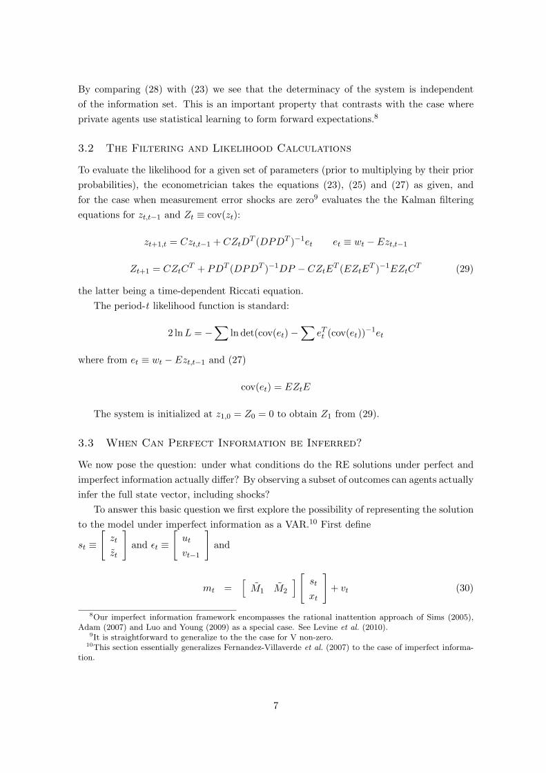
3.2 The Filtering and Likelihood Calculations
To evaluate the likelihood for a given set of parameters (prior to multiplying by their prior
probabilities), the econometrician takes the equations (23), (25) and (27) as given, and
for the case when measurement error shocks are zero9 evaluates the the Kalman filtering
equations for zt,t−1 and Zt ≡ cov(zt):
zt+1,t = Czt,t−1 + CZtDT (DPDT )−1et et ≡ wt − Ezt,t−1
Zt+1 = CZtCT + PDT (DPDT )−1DP − CZtE
T (EZtET )−1EZtC
T (29)
the latter being a time-dependent Riccati equation.
The period-t likelihood function is standard:
2 lnL = −∑
ln det(cov(et)−∑
eTt (cov(et))−1et
where from et ≡ wt − Ezt,t−1 and (27)
cov(et) = EZtE
The system is initialized at z1,0 = Z0 = 0 to obtain Z1 from (29).
3.3 When Can Perfect Information be Inferred?
We now pose the question: under what conditions do the RE solutions under perfect and
imperfect information actually differ? By observing a subset of outcomes can agents actually
infer the full state vector, including shocks?
To answer this basic question we first explore the possibility of representing the solution
to the model under imperfect information as a VAR.10 First define
st ≡
[zt
zt
]and ϵt ≡
[ut
vt−1
]and
mt =[M1 M2
] [ st
xt
]+ vt (30)
8Our imperfect information framework encompasses the rational inattention approach of Sims (2005),Adam (2007) and Luo and Young (2009) as a special case. See Levine et al. (2010).
9It is straightforward to generalize to the the case for V non-zero.10This section essentially generalizes Fernandez-Villaverde et al. (2007) to the case of imperfect informa-
tion.
7
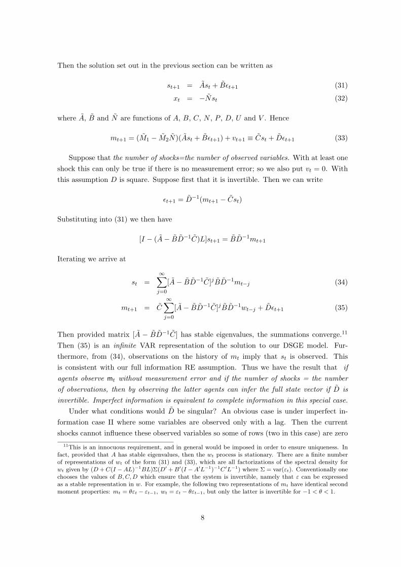
Then the solution set out in the previous section can be written as
st+1 = Ast + Bϵt+1 (31)
xt = −Nst (32)
where A, B and N are functions of A, B, C, N , P , D, U and V . Hence
mt+1 = (M1 − M2N)(Ast + Bϵt+1) + vt+1 ≡ Cst + Dϵt+1 (33)
Suppose that the number of shocks=the number of observed variables. With at least one
shock this can only be true if there is no measurement error; so we also put vt = 0. With
this assumption D is square. Suppose first that it is invertible. Then we can write
ϵt+1 = D−1(mt+1 − Cst)
Substituting into (31) we then have
[I − (A− BD−1C)L]st+1 = BD−1mt+1
Iterating we arrive at
st =
∞∑j=0
[A− BD−1C]jBD−1mt−j (34)
mt+1 = C∞∑j=0
[A− BD−1C]jBD−1wt−j + Dϵt+1 (35)
Then provided matrix [A − BD−1C] has stable eigenvalues, the summations converge.11
Then (35) is an infinite VAR representation of the solution to our DSGE model. Fur-
thermore, from (34), observations on the history of mt imply that st is observed. This
is consistent with our full information RE assumption. Thus we have the result that if
agents observe mt without measurement error and if the number of shocks = the number
of observations, then by observing the latter agents can infer the full state vector if D is
invertible. Imperfect information is equivalent to complete information in this special case.
Under what conditions would D be singular? An obvious case is under imperfect in-
formation case II where some variables are observed only with a lag. Then the current
shocks cannot influence these observed variables so some of rows (two in this case) are zero
11This is an innocuous requirement, and in general would be imposed in order to ensure uniqueness. Infact, provided that A has stable eigenvalues, then the wt process is stationary. There are a finite numberof representations of wt of the form (31) and (33), which are all factorizations of the spectral density forwt given by (D+C(I −AL)−1BL)Σ(D′ +B′(I −A′L−1)−1C′L−1) where Σ = var(εt). Conventionally onechooses the values of B,C,D which ensure that the system is invertible, namely that ε can be expressedas a stable representation in w. For example, the following two representations of mt have identical secondmoment properties: mt = θεt − εt−1, wt = εt − θεt−1, but only the latter is invertible for −1 < θ < 1.
8
meaning D is not invertible. In our model then, both these sufficient conditions for imper-
fect information collapsing to the perfect information case do not hold, so we can expect
differences between the two cases.12
4 Bayesian Estimation
In the same year that Blanchard and Kahn (1980) provide a general solution for a linear
model under RE in the state space form, Sims (1980) suggests the use of Bayesian methods
for solving multivariate systems. This leads to the development of Bayesian VAR (BVAR)
models (Doan et al. (1984)), and, during the 1980s, the extensive development and appli-
cation of Kalman filtering-based state space systems methods in statistics and economics
(Aoki (1987), Harvey (1989)).
Modern DSGE methods further enhance this Kalman filtering based Bayesian VAR state
space model with Monte-Carlo Markov Chain (MCMC) optimising, stochastic simulation
and importance-sampling (Metropolis-Hastings (MH) or Gibbs) algorithms. The aim of this
enhancement is to provide the optimised estimates of the expected values of the currently
unobserved, or the expected future values of the variables and of the relational parameters
together with their posterior probability density distributions (Geweke (1999)). It has been
shown that DSGE estimates are generally superior, especially for the longer-term predictive
estimation than the VAR (but not BVAR) estimates (Smets and Wouters (2007)), and
particularly in data-rich conditions (Boivin and Giannoni (2005)).
The crucial aspect is that agents in DSGE models are forward-looking. As a con-
sequence, any expectations that are formed are dependent on the agents’ information set.
Thus unlike a backward-looking engineering system, the information set available will affect
the path of a DSGE system.
The Bayesian approach uses the Kalman filter to combine the prior distributions for
the individual parameters with the likelihood function to form the posterior density. This
posterior density can then be obtained by optimizing with respect to the model parameters
through the use of the Monte-Carlo Markov Chain sampling methods. Four variants of
our linearized model are estimated using the Dynare software (Juillard (2003)), which has
been extended by the paper’s authors to allow for imperfect information on the part of the
private sector.
In the process of parameter estimation, the mode of the posterior is first estimated using
Chris Sim’s csminwel after the models’ log-prior densities and log-likelihood functions are
obtained by running the Kalman recursion and are evaluated and maximized. Then a
sample from the posterior distribution is obtained with the Metropolis-Hasting algorithm
using the inverse Hessian at the estimated posterior mode as the covariance matrix of the
jumping distribution. The scale used for the jumping distribution in the MH is set in order
12In fact many NK DSGE models do have the property that the number of shocks equal the number ofobservable and the latter are current values without lags - for example Smets and Wouters (2003).
9
to allow a good acceptance rate (20%-40%). A number of parallel Markov chains of 100000
runs each are run for the MH in order to ensure the chains converge. The first 25% of
iterations (initial burn-in period) are discarded in order to remove any dependence of the
chain from its starting values.
4.1 Data and Priors
To estimate the system, we use three macro-economic observables at quarterly frequency
for the US: real GDP, the GDP deflator and the nominal interest rate. Since the variables
in the model are measured as deviations from a constant steady state, the time series are
simply de-trended against a linear trend in order to obtain approximately stationary data.
As a robustness check we also ran estimations using an output series detrending output with
a linear-quadratic trend. Following Smets and Wouters (2003), all variables are treated as
deviations around the sample mean. Real variables are measured in logarithmic deviations
from linear trends, in percentage points, while inflation (the GDP deflator) and the nominal
interest rate are detrended by the same linear trend in inflation and converted to quarterly
rates. The estimation results are based on a sample from 1981:1 to 2006:4.
The values of priors are taken from Levin et al. (2006) and Smets and Wouters (2007).
Table 8 in Appendix D provides an overview of the priors used for each model variant
described below. In general, inverse gamma distributions are used as priors when non-
negativity constraints are necessary, and beta distributions for fractions or probabilities.
Normal distributions are used when more informative priors seem to be necessary. We
use the same prior means as in previous studies and allow for larger standard deviations,
i.e. less informative priors, in particular for the habit parameter and price indexation. The
priors on ξ are the exception and based on Smets and Wouters (2007) with smaller standard
deviations. Also, for the parameters γ, hC , ξ and ϱ we centre the prior density in the middle
of the unit interval. The priors related to the process for the price mark-up shock are
taken from Smets and Wouters (2007). The priors for µ1, µ2, µ3, λh, λf are also assumed
beta distributed with means 0.5 and standard deviations 0.2. Three of the structural
parameters are kept fixed in the estimation procedure. These calibrated parameters are
β = 0.99; L = 0.4, cy = 0.6.
4.2 Estimation Results
We consider 4 model variants: GH (γ, hC > 0), G (hC = 0), H (γ = 0) and Z (zero persis-
tence or γ = hC = 0). Then for each model variant we examine three information sets: first
we make the assumption that private agents are better informed than the econometricians
(the standard asymmetric information case in the estimation literature) – the Asymmetric
Information (AI) case. Then we examine two symmetric information sets for both econo-
metrician and private agents: Imperfect Information without measurement error on the
three observables rt, πt, yt (II) and measurement error on two observables πt, yt (IIME).
10
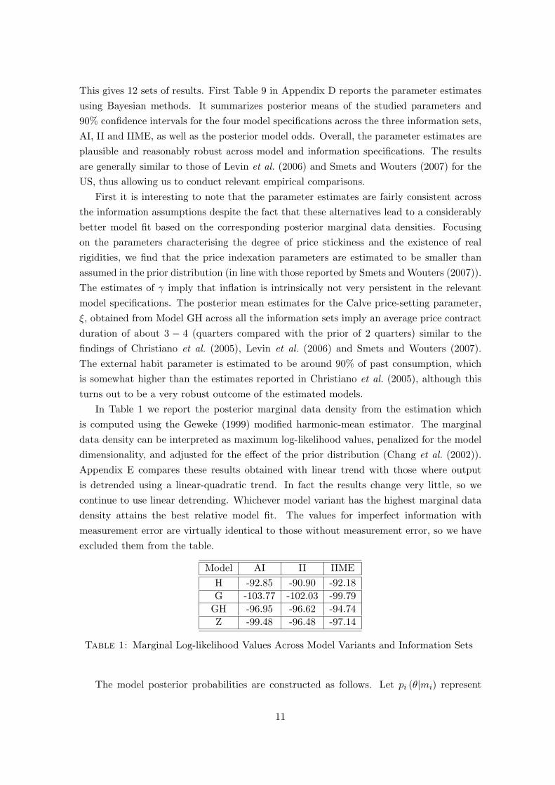
This gives 12 sets of results. First Table 9 in Appendix D reports the parameter estimates
using Bayesian methods. It summarizes posterior means of the studied parameters and
90% confidence intervals for the four model specifications across the three information sets,
AI, II and IIME, as well as the posterior model odds. Overall, the parameter estimates are
plausible and reasonably robust across model and information specifications. The results
are generally similar to those of Levin et al. (2006) and Smets and Wouters (2007) for the
US, thus allowing us to conduct relevant empirical comparisons.
First it is interesting to note that the parameter estimates are fairly consistent across
the information assumptions despite the fact that these alternatives lead to a considerably
better model fit based on the corresponding posterior marginal data densities. Focusing
on the parameters characterising the degree of price stickiness and the existence of real
rigidities, we find that the price indexation parameters are estimated to be smaller than
assumed in the prior distribution (in line with those reported by Smets and Wouters (2007)).
The estimates of γ imply that inflation is intrinsically not very persistent in the relevant
model specifications. The posterior mean estimates for the Calve price-setting parameter,
ξ, obtained from Model GH across all the information sets imply an average price contract
duration of about 3 − 4 (quarters compared with the prior of 2 quarters) similar to the
findings of Christiano et al. (2005), Levin et al. (2006) and Smets and Wouters (2007).
The external habit parameter is estimated to be around 90% of past consumption, which
is somewhat higher than the estimates reported in Christiano et al. (2005), although this
turns out to be a very robust outcome of the estimated models.
In Table 1 we report the posterior marginal data density from the estimation which
is computed using the Geweke (1999) modified harmonic-mean estimator. The marginal
data density can be interpreted as maximum log-likelihood values, penalized for the model
dimensionality, and adjusted for the effect of the prior distribution (Chang et al. (2002)).
Appendix E compares these results obtained with linear trend with those where output
is detrended using a linear-quadratic trend. In fact the results change very little, so we
continue to use linear detrending. Whichever model variant has the highest marginal data
density attains the best relative model fit. The values for imperfect information with
measurement error are virtually identical to those without measurement error, so we have
excluded them from the table.
Model AI II IIME
H -92.85 -90.90 -92.18
G -103.77 -102.03 -99.79
GH -96.95 -96.62 -94.74
Z -99.48 -96.48 -97.14
Table 1: Marginal Log-likelihood Values Across Model Variants and Information Sets
The model posterior probabilities are constructed as follows. Let pi (θ|mi) represent
11
the prior distribution of the parameter vector θ ∈ Θ for some model mi ∈ M and let
L (y|θ,mi) denote the likelihood function for the observed data y ∈ Y conditional on the
model and the parameter vector. Then the joint posterior distribution of θ for model mi
combines the likelihood function with the prior distribution:
pi (θ|y,mi) ∝ L (y|θ,mi) pi (θ|mi)
Bayesian inference also allows a framework for comparing alternative and potentially
misspecified models based on their marginal likelihood. For a given model mi ∈ M and
common dataset, the latter is obtained by integrating out vector θ,
L (y|mi) =
∫ΘL (y|θ,mi) p (θ|mi) dθ
where pi (θ|mi) is the prior density for model mi, and L (y|mi) is the data density for
model mi given parameter vector θ. To compare models (say, mi and mj) we calculate
the posterior odds ratio which is the ratio of their posterior model probabilities (or Bayes
Factor when the prior odds ratio, p(mi)p(mj)
, is set to unity):
POi,j =p(mi|y)p(mj |y)
=L(y|mi)p(mi)
L(y|mj)p(mj)(36)
BFi,j =L(y|mi)
L(y|mj)=
exp(LL(y|mi))
exp(LL(y|mj))(37)
in terms of the log-likelihoods. Components (36) and (37) provide a framework for com-
paring alternative and potentially misspecified models based on their marginal likelihood.
Such comparisons are important in the assessment of rival models.
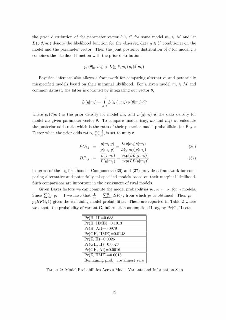
Given Bayes factors we can compute the model probabilities p1, p2, · · ·pn for n models.
Since∑n
i=1 pi = 1 we have that 1p1
=∑n
i=2BFi,1, from which p1 is obtained. Then pi =
p1BF (i, 1) gives the remaining model probabilities. These are reported in Table 2 where
we denote the probability of variant G, information assumption II say, by Pr(G, II) etc.
Pr(H, II)=0.688
Pr(H, IIME)=0.1913
Pr(H, AI)=0.0979
Pr(GH, IIME)=0.0148
Pr(Z, II)=0.0026
Pr(GH, II)=0.0023
Pr(GH, AI)=0.0016
Pr(Z, IIME)=0.0013
Remaining prob. are almost zero
Table 2: Model Probabilities Across Model Variants and Information Sets
12

Tables 1 and 2 reveal that a combination of Model H and with information set II
outperforms the same with information set AI by a Bayes factor of approximately 7. For all
models II ≻ AI in terms of LL. This is a striking result; although informational consistency
in intuitively appealing there is no inevitability that models that assume this will perform
better in LL terms than the traditional assumption of AI. By the same token introducing
measurement error into the private sector’s observations (information set IIME) is not
bound to improve performance and indeed we see that the IIME case does not uniformly
improve LL performance except for models G and GH where we do see IIME ≻ II ≻ AI.
Our model comparison analysis contains two other important results. First, uniformly
across all information sets indexation does not improve the model fit, but the existence
of habit is crucial. The poor performance of indexation is in a sense encouraging as this
feature of the NK is ad hoc and vulnerable to the Lucas critique. The existence of habit by
contrast is a plausible formulation of utility that addresses issues examined in the happiness
literature.13 Second, the II as compared with AI specification leads to significantly better
fit for Model Z, and a better improvement than for the other three model variants. Model
Z we recall is the model with zero persistence mechanisms. Its substantial improvement
of performance on introducing II on the part of the private sector confirms our earlier
analytical results that show how II introduces endogenous persistence. But where other
persistence mechanisms habit and indexation exist in models H and GH these to some
extent overshadow the improvement brought by II.
5 The General Set-Up and Optimal Policy Problem
This section describes the general set-up that applies irrespective of the informational as-
sumptions. Removing the estimated rule (12), for a given set of observed policy instruments
wt we now consider a linearized model in a general state-space form:[zt+1
Etxt+1
]= A1
[zt
xt
]+A2
[Etzt
Etxt
]+Bwt +
[ut+1
0
](38)
where zt, xt are vectors of backward and forward-looking variables, respectively, wt is a
vector of policy variables, and ut is a i.d. zero mean shock variable with covariance matrix
Σu; a more general setup allows for shocks to the equations involving expectations. In
addition for the imperfect information case, we assume that agents all make the same
observations at time t, which are still given by (20).
Define target variables st by
st = Jyt +Hwt (39)
13In particular the “Easterin paradox”, Easterlin (2003). See also Layard (2006) and Choudhary et al.(2011) for the role of external habit in the explanation of the paradox.
13
Then the policy-maker’s loss function at time t by
Ωt =1
2
∞∑τ=0
βt[sTt+τQ1st+τ + wTt+τQ2wt+τ ] (40)
This could be an ad hoc loss function or a large distortions approximation to the household’s
utility as described in Levine et al. (2008a). Substituting (39) into (40) results in the
following form of the loss function used subsequently in the paper
Ωt =1
2
∞∑i=0
βt[yTt+τQyt+τ + 2yTt+τUwt+τ + wTt+τRwt+τ ] (41)
where Q = JTQ1M , U = JTQ1H, R = Q2 + HTQ1H, Q1 and Q2 are symmetric and
non-negative definite, R is required to be positive definite and β ∈ (0, 1) is discount factor.
For the literature described in the introduction, rational expectations are formed as-
suming the following information sets:
1. For perfect information the private sector and policymaker/modeller have the follow-
ing information set:
It = zτ , xτ, τ ≤ t;A1, A2, B,Σu, [Q,U,R, β] or the monetary rule
2. For symmetric imperfect information (see Pearlman (1992), Svensson and Woodford
(2003) and for Bayesian estimation, Levine et al. (2010)):
It = mτ, τ ≤ t;A1, A2, B,M1,M2, L,Σu,Σv, [Q,U,R, β] or the monetary rule.
3. For the first category of asymmetric imperfect information (see Svensson and Wood-
ford (2001), Aoki (2003), Aoki (2006) and standard Bayesian estimation):
Ipst = It = zτ , xτ, τ ≤ t;A1, A2, B,Σu, [Q,U,R, β] or the monetary rule for the pri-
vate sector and
Ipolt = mτ, τ ≤ t;A1, A2, B,M1,M2, L,Σu,Σv, [Q,U,R, β] or the monetary rule for
the policymaker.
4. For the second category of asymmetric imperfect information (see Cukierman and
Meltzer (1986), Faust and Svensson (2001), Faust and Svensson (2002)) and (Melecky
et al. (2008)):
Ipolt = mτ, τ ≤ t;A1, A2, B,M1,M2, L,Σu,Σv, [Q,U,R, β] or the monetary rule for
the policymaker sector and
Ipst = mτ, τ ≤ t;A1, A2, B,M1,M2, L,Σu,Σv for the private sector.
In the rest of the paper we confine ourselves to information set 1 for perfect information
and information set 2 for imperfect information. Information set 3 is incompatible with the
ICP. Information set 4 is however compatible and is needed to address the issue of optimal
ambiguity. However this interesting case is beyond the scope of this paper.
14

6 Optimal Policy Under Perfect Information
Under perfect information,
[Etzt
Etxt
]=
[zt
xt
]. Let A ≡ A1 + A2 and first consider the
purely deterministic problem with a model then in state-space form:[zt+1
xet+1,t
]= A
[zt
xt
]+Bwt (42)
where zt is an (n − m) × 1 vector of predetermined variables including non-stationary
processed, z0 is given, wt is a vector of policy variables, xt is an m × 1 vector of non-
predetermined variables and xet+1,t denotes rational (model consistent) expectations of xt+1
formed at time t. Then xet+1,t = xt+1 and letting yTt =[zTt xTt
](42) becomes
yt+1 = Ayt +Bwt (43)
The procedures for evaluating the three policy rules are outlined in the rest of this
section (or Currie and Levine (1993) for a more detailed treatment).
6.1 The Optimal Policy with Commitment
Consider the policy-maker’s ex-ante optimal policy at t = 0. This is found by minimizing Ω0
given by (41) subject to (43) and (39) and given z0. We proceed by defining the Hamiltonian
Ht(yt, yt+1, µt+1) =1
2βt(yTt Qyt + 2yTt Uwt + wT
t Rwt) + µt+1(Ayt +Bwt − yt+1) (44)
where µt is a row vector of costate variables. By standard Lagrange multiplier theory we
minimize
L0(y0, y1, . . . , w0, w1, . . . , µ1, µ2, . . .) =∞∑t=0
Ht (45)
with respect to the arguments of L0 (except z0 which is given). Then at the optimum,
L0 = Ω0.
Redefining a new costate column vector pt = β−tµTt , the first-order conditions lead to
wt = −R−1(βBTpt+1 + UT yt) (46)
βATpt+1 − pt = −(Qyt + Uwt) (47)
Substituting (46) into (43)) we arrive at the following system under control[I βBR−1BT
0 β(AT − UR−1BT )
][yt+1
pt+1
]=
[A−BR−1UT 0
−(Q− UR−1UT I
][yt
pt
](48)
To complete the solution we require 2n boundary conditions for (48). Specifying z0
15
gives us n−m of these conditions. The remaining condition is the ‘transversality condition’
limt→∞
µTt = lim
t→∞βtpt = 0 (49)
and the initial condition
p20 = 0 (50)
where pTt =[pT1t p
T2t
]is partitioned so that p1t is of dimension (n−m)× 1. Equation (39),
(46), (48) together with the 2n boundary conditions constitute the system under optimal
control.
Solving the system under control leads to the following rule
wt = −F
[I 0
−N21 −N22
][zt
p2t
]≡ D
[zt
p2t
]= −F
[zt
x2t
](51)
where [zt+1
p2t+1
]=
[I 0
S21 S22
]G
[I 0
−N21 −N22
][zt
p2t
]≡ H
[zt
p2t
](52)
N =
[S11 − S12S
−122 S21 S12S
−122
−S−122 S21 S−1
22
]=
[N11 N12
N21 N22
](53)
xt = −[N21 N22
] [ zt
p2t
](54)
where F = −(R+BTSB)−1(BTSOPTA+ UT ), G = A−BF and
S =
[S11 S12
S21 S22
](55)
partitioned so that S11 is (n − m) × (n − m) and S22 is m × m is the solution to the
steady-state Ricatti equation
S = Q− UF − F TUT + F TRF + β(A−BF )TS(A−BF ) (56)
The welfare loss for the optimal policy (OPT) at time t is
ΩOPTt = −1
2(tr(N11Zt) + tr(N22p2tp
T2t)) (57)
where Zt = ztzTt . To achieve optimality the policy-maker sets p20 = 0 at time t = 0.14 At
14Noting from (54) that for the optimal policy we have xt = −N21zt −N22p2t, the optimal policy “froma timeless perspective” proposed by Woodford (2003) replaces the initial condition for optimality p20 = 0with Jx0 = −N21z0 − N22p20 where J is some 1 × m matrix. Typically in New Keynesian models theparticular choice of condition is π0 = 0 thus avoiding any once-and-for-all initial surprise inflation. Thisinitial condition applies only at t = 0 and only affects the deterministic component of policy and not thestochastic, stabilization component.
16
time t > 0 there exists a gain from reneging by resetting p2t = 0. It can be shown that
N11 < 0 and N22 < 0.15, so the incentive to renege exists at all points along the trajectory
of the optimal policy. This is the time-inconsistency problem.
6.2 The Dynamic Programming Discretionary Policy
To evaluate the discretionary (time-consistent) policy we rewrite the welfare loss Ωt given
by (41) as
Ωt =1
2[yTt Qyt + 2yTt Uwt + wT
t Rwt + βΩt+1] (58)
The dynamic programming solution then seeks a stationary solution of the form wt =
−Fzt in which Ωt is minimized at time t subject to (1) in the knowledge that a similar
procedure will be used to minimize Ωt+1 at time t+ 1.
Suppose that the policy-maker at time t expects a private-sector response from t + 1
onwards, determined by subsequent re-optimization, of the form
xt+τ = −Nt+1zt+τ , τ ≥ 1 (59)
The loss at time t for the ex ante optimal policy was from (57) found to be a quadratic
function of xt and p2t. We have seen that the inclusion of p2t was the source of the time
inconsistency in that case. We therefore seek a lower-order controller
wt = −F zt (60)
with the welfare loss in zt only. We then write Ωt+1 = 12z
Tt+1S
TCTt+1 zt+1 in (58). This leads
to the following iterative process for Ft
wt = −Ftzt (61)
where
Ft = (Rt + λBTt S
TCTt+1 Bt)
−1(UTt + βB
Tt S
TCTt+1 At)
Rt = R+KTt Q22Kt + U2TKt +KT
t U2
Kt = −(A22 +Nt+1A12)−1(Nt+1B
1 +B2)
Bt = B1 +A12Kt
U t = U1 +Q12Kt + JTt U
2 + JTt Q22Jt
J t = −(A22 +Nt+1A12)−1(Nt+1A11 +A12)
15See Currie and Levine (1993), chapter 5.
17
At = A11 +A12Jt
STCTt = Qt − U tFt − F T
t UT+ F
Tt RtFt + β(At −BtFt)
TSTCTt+1 (At −BtF t)
Qt = Q11 + JTt Q21 +Q12Jt + JT
t Q22Jt
Nt = −Jt +KtFt
where B =
[B1
B2
], U =
[U1
U2
], A =
[A11 A12
A21 A22
], and Q similarly are partitioned con-
formably with the predetermined and non-predetermined components of the state vector.
The sequence above describes an iterative process for Ft, Nt, and STCTt starting with
some initial values for Nt and STCTt . If the process converges to stationary values, F,N
and S say, then the time-consistent feedback rule is wt = −F zt with loss at time t given by
ΩTCTt =
1
2zTt S
TCT zt =1
2tr(STCTZt) (62)
6.3 Optimized Simple Rules
We now consider simple sub-optimal rules of the form
wt = Dyt = D
[zt
xt
](63)
where D is constrained to be sparse in some specified way. Rule (63) can be quite general.
By augmenting the state vector in an appropriate way it can represent a PID (proportional-
integral-derivative)controller.
Substituting (63) into (41) gives
Ωt =1
2
∞∑i=0
βtyTt+iPt+iyt+i (64)
where P = Q + UD +DTUT +DTRD. The system under control (42), with wt given by
(63), has a rational expectations solution with xt = −Nzt where N = N(D). Hence
yTt P yt = zTt T zt (65)
where T = P11 −NTP21 − P12N +NTP22N , P is partitioned as for S in (55) onwards and
zt+1 = (G11 −G12N)zt (66)
where G = A+BD is partitioned as for P . Solving (66) we have
zt = (G11 −G12N)tz0 (67)
18

Hence from (68), (65) and (67) we may write at time t
ΩSIMt =
1
2zTt V zt =
1
2tr(V Zt) (68)
where Zt = ztzTt and V LY A satisfies the Lyapunov equation
V LY A = T +HTV LY AH (69)
where H = G11 − G12N . At time t = 0 the optimized simple rule is then found by
minimizing Ω0 given by (68) with respect to the non-zero elements of D given z0 using a
standard numerical technique. An important feature of the result is that unlike the previous
solution the optimal value of D, D∗ say, is not independent of z0. That is to say
D∗ = D∗(z0)
6.4 The Stochastic Case
Consider the stochastic generalization of (42)[zt+1
xet+1,t
]= A
[zt
xt
]+Bwt +
[ut
0
](70)
where ut is an n × 1 vector of white noise disturbances independently distributed with
cov(ut) = Σ. Then, it can be shown that certainty equivalence applies to all the policy
rules apart from the simple rules (see Currie and Levine (1993)). The expected loss at time
t is as before with quadratic terms of the form zTt Xzt = tr(Xzt, ZTt ) replaced with
Et
(tr
[X
(ztz
Tt +
∞∑i=1
βtut+iuTt+i
)])= tr
[X
(zTt zt +
λ
1− λΣ
)](71)
where Et is the expectations operator with expectations formed at time t.
Thus for the optimal policy with commitment (57) becomes in the stochastic case
ΩOPTt = −1
2tr
(N11
(Zt +
β
1− βΣ
)+N22p2tp
T2t
)(72)
For the time-consistent policy (62) becomes
ΩTCTt = −1
2tr
(S
(Zt +
β
1− βΣ
))(73)
and for the simple rule, generalizing (68)
ΩSIMt = −1
2tr
(V LY A
(Zt +
β
1− βΣ
))(74)
19
The optimized simple rule is found at time t = 0 by minimizing ΩSIM0 given by (74).
Now we find that
D∗ = D∗(z0z
T0 +
β
1− βΣ
)(75)
or, in other words, the optimized rule depends both on the initial displacement z0 and on
the covariance matrix of disturbances Σ.
A very important feature of optimized simple rules is that unlike their optimal com-
mitment or optimal discretionary counterparts they are not certainty equivalent. In fact
if the rule is designed at time t = 0 then D∗ = f∗(Z0 +
β1−βΣ
)and so depends on the
displacement z0 at time t = 0 and on the covariance matrix of innovations Σ = cov(ϵt).
From non-certainty equivalence it follows that if the simple rule were to be re-designed at
ant time t > 0, since the re-optimized D∗ will then depend on Zt the new rule will differ
from that at t = 0. This feature is true in models with or without rational forward-looking
behaviour and it implies that simple rules are time-inconsistent even in non-RE models.
7 Optimal Policy Under Imperfect Information
Here we assume that that there is a set of measurements as described above in section 3.
The following is a summary of the solution provided by Pearlman (1992), with some details
provided in Appendix C. It can be shown that the estimate for zt at time t, denoted by zt,t
can be expressed in terms of the innovations process zt − zt,t−1 as
zt,t = zt,t−1 + PDT (DPDT + V )−1(D(zt − zt,t−1) + vt) (76)
where D = M11 −M1
2 (A122)
−1A121, M
1 = [M11 ,M
12 ], M
2 = [M21 ,M
22 ] partitioned conformably
with [zTt , xTt ]
T , and P is the solution of the Riccati equation describing the Kalman Filter
P = APAT −APDT (DPDT + V )−1DPAT +Σ (77)
where A = A111−A1
12(A122)
−1A121. One can also show that zt− zt,t and zt,t are orthogonal in
expectations. Note that this Riccati equation is independent of policy. We may then write
the expected utility as
1
2Et
[ ∞∑i=0
βt(yTt+τ,t+τQyt+τ,t+τ + 2yTt+τ,t+τUwt+τ + wTt+τRwt+τ
+ (yt+τ − yt+τ,t+τ )TQ(yt+τ − yt+τ,t+τ ))
](78)
where we note that wt+τ is dependent only on current and past yt+s,t+s. This is minimized
subject to the dynamics[zt+1,t+1
Etxt+1,t+1
]= (A1 +A2)
[zt,t
xt,t
]+Bwt +
[zt+1,t+1 − zt+1,t
0
](79)
20

which represents the expected dynamics of the system (where we note by the chain rule
that Etxt+1,t+1 , Et[Et+1xt+1] = Etxt+1. Note that cov(zt+1,t+1−zt+1,t) = PDT (DPDT +
V )−1DP and cov(zt+1 − zt+1,t+1) = P − PDT (DPDT + V )−1DP , P .
Taking time-t expectations of the equation involving Etxt+1 and subtracting from the
original yields:
0 = A112(zt − zt,t) +A1
22(xt − xt,t) (80)
Furthermore, as in Pearlman (1992) we can show that certainty equivalence holds for both
the fully optimal and the time consistent solution, it is straightforward to show that ex-
pected welfare for each of the regimes is given by
W J =zT0,0SJz0,0 +
λ
1− λtr(SJPDT (DPDT + V )−1DP
)+
1
1− λtr(Q11 −Q12(A
122)
−1A121 − (A1
21)T (A1
22)−TQ21 + (A1
21)T (A1
22)−TQ22(A
122)
−1A121
)P
(81)
where J =OPT, TCT, SIM; the second term is the expected value of the first three terms
of (78) under each of the rules, and the final term is independent of the policy rule, and is
the expected value of the final term of (78), utilising (80). Also note that from the perfect
information case in the previous subsection:
SOPT = N11 ≡ S11 − S12S−122 S21 (82)
• Sij are the partitions of S, the Ricatti matrix used to calculate the welfare loss under
optimal policy with commitment.
• STCT is used to calculate the welfare loss in the time consistent solution algorithm.
• SSIM = V LY A is calculated from the Lyapunov equation used to calculate the welfare
under the optimized simple rule.
In the special case of perfect information, M1 = I, M2 = vt = V so that D = E = I.
It follows that P = 0 and the last term in (81) disappears. Moreover P = Σ, z0,0 = z0
and (81) reduces to the welfare loss expressions obtained previously. Thus the effect of
imperfect information is to introduce a new term into the welfare loss that depends only on
the model’s transmission of policy but is independent of that policy and to modify the first
policy-dependent term by an effect that depends on the solution P to the Ricatti equation
associated with the Kalman Filter.
8 Optimal Monetary Policy in the NK Model: Results
This section sets out numerical results for optimal policy under commitment, optimal dis-
cretionary (or time consistent) policy and for a optimized simple Taylor rule. The model is
21
the estimated form of the best-fitting one, namely model H. For the first set of results we
ignore ZLB considerations. The questions we pose are first, what are the welfare costs as-
sociated with the private sector possesses only imperfect information of the state variables;
second, what are the implications of imperfect information for the gains from commitment
and third, how does imperfect information affect the form of optimized Taylor rules.
This section addresses all these questions. We examine two imperfect information sets.
Imperfect Information Set I: This consists of the current and past values of output,
inflation and the interest rate In this scenario the private sector must infer the shocks from
its observations.
Imperfect Information Set II: As for I but output and inflation are only observed with
a lag, but the current interest rate is observed.
We considered simple inflation targeting rules that respond only to inflation.16 The
corresponding forms of the rules for the two information sets are
rt = ρrrt−1 + θππt (83)
for perfect information and information set I, and either
rt = ρrrt−1 + θπEtπt (Form A) (84)
or
rt = ρrrt−1 + θππt−1 (Form B) (85)
for information set II.
With this choice of Taylor rule the case where ρr = 1 is of particular interest as this
then corresponds to a price-level rule. There has been a recent interest in the case for price-
level rather than inflation stability. Gaspar et al. (2010) provide an excellent review of this
literature. The basic difference between the two regimes in that under an inflation targeting
mark-up shock leads to a commitment to use the interest rate to accommodate an increase
in the inflation rate falling back to its steady state. By contrast a price-level rule commits
to a inflation rate below its steady state after the same initial rise. Under inflation targeting
one lets bygones be bygones allowing the price level to drift to a permanently different price-
level path whereas price-level targeting restores the price level to its steady state path. The
16We also considered the following simple rules that responding to both inflation and output:
rt = ρrrt−1 + θππt + θyyt
for perfect information and information set I, and either
rt = ρrrt−1 + θπEtπt + θyEtyt (Form A)
rt = ρrrt−1 + θππt−1 + θyyt−1 (Form B)
for information set II. However the results were very similar with a very small weight on output.
22

latter can lower inflation variance and be welfare enhancing because forward-looking price-
setters anticipates that a current increase in the general price level will be undone giving
them an incentive to moderate the current adjustment of its own price. In our results
we will see if price-level targeting is indeed welfare optimal across different information
assumptions.
8.1 Optimal Policy without Zero Lower Bound Considerations
Results are presented for a loss function that is formally a quadratic approximation about
the steady state of the Lagrangian, and which represents the true approximation about the
fully optimal solution. This welfare-based loss function has been obtained numerically.
A permanent drop in consumption of 0.1464% produces a welfare loss per period of 100.
So from Table 3 we can see (a) that the gains from commitment are very small under any
information set; (b) that imperfect information in the form of only observing a subset of
current state variables (information set I) imposes only a tiny welfare loss, whereas if only
lagged output and inflation are observed, the losses are significant, and are of the order of
0.11% consumption equivalent.
Simple rules are able to quite well replicate the welfare losses under the fully optimal
solution, albeit with Simple Rule A requiring a large weight θπ = 16 on inflation, and ρr =
1.0 on lagged interest rates (virtually the same for all information sets). This derivative rule
in inflation is equivalent to a price level rule. For Simple Rule B, with lagged information
on inflation, the welfare loss is similar but achieved with weights θπ = 2.26 and ρr = 0.6,
so the price level rule does not apply in this case and the II with only lagged observations
of output and inflation has important implications for the form of the optimized rule.
Information Information Set Optimal Time Consistent Simple Rule A Simple Rule B
Perfect Full state vector 20.06 21.22 21.39 n. a.
Imperfect I It = [yt, πt, rt] 20.45 21.62 20.46 n. a.
Imperfect II It = [yt−1, πt−1, rt] 95.61 97.6 95.62 95.85
Table 3: Welfare Costs per period of Imperfect Information without ZLB Considerations
Information Information Set Simple Rule A Simple Rule B[ρr, θπ] [ρr, θπ]
Perfect Full state vector [1, 16] n. a.
Imperfect I It = [yt, πt, rt] [1,16] n. a.
Imperfect II It = [yt−1, πt−1, rt] [1, 16.5] [0.6, 2.26]
Table 4: Optimized Coefficients in Simple Rules without ZLB Considerations
23
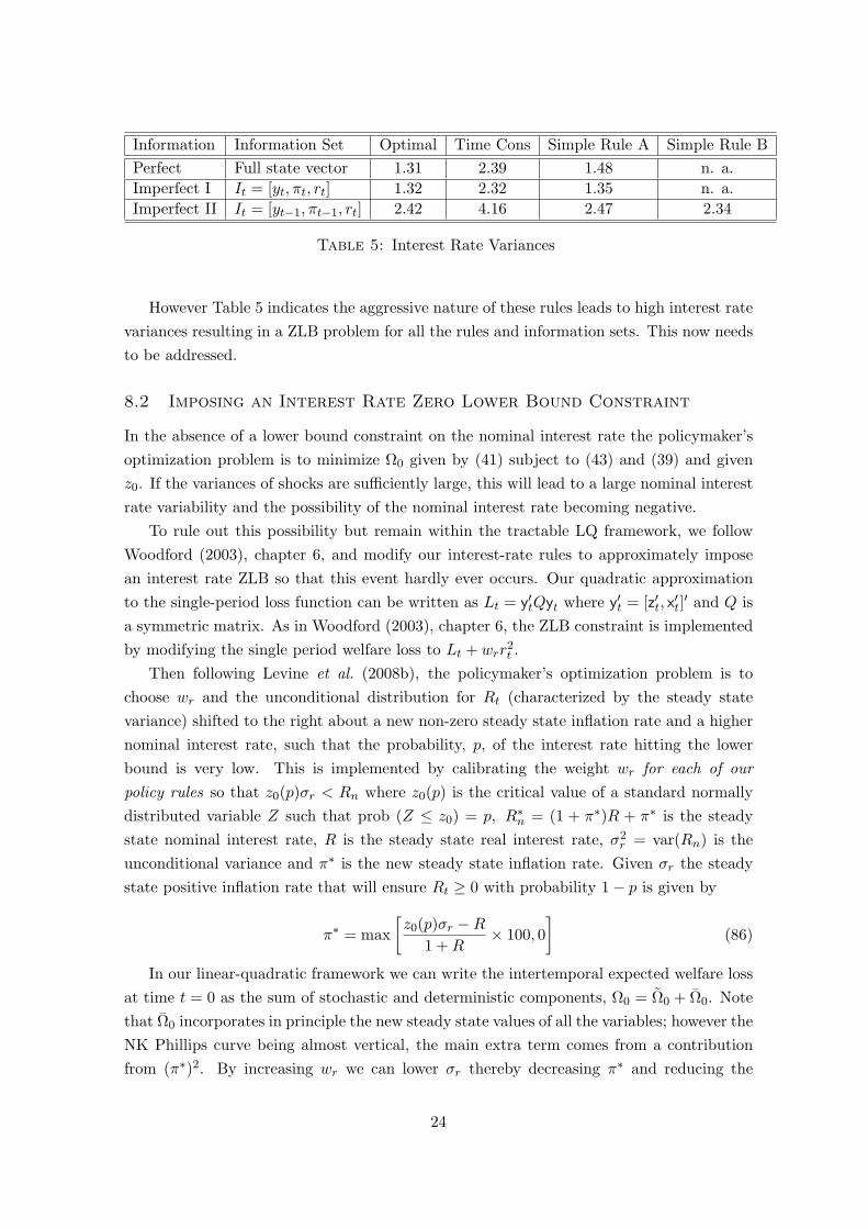
Information Information Set Optimal Time Cons Simple Rule A Simple Rule B
Perfect Full state vector 1.31 2.39 1.48 n. a.
Imperfect I It = [yt, πt, rt] 1.32 2.32 1.35 n. a.
Imperfect II It = [yt−1, πt−1, rt] 2.42 4.16 2.47 2.34
Table 5: Interest Rate Variances
However Table 5 indicates the aggressive nature of these rules leads to high interest rate
variances resulting in a ZLB problem for all the rules and information sets. This now needs
to be addressed.
8.2 Imposing an Interest Rate Zero Lower Bound Constraint
In the absence of a lower bound constraint on the nominal interest rate the policymaker’s
optimization problem is to minimize Ω0 given by (41) subject to (43) and (39) and given
z0. If the variances of shocks are sufficiently large, this will lead to a large nominal interest
rate variability and the possibility of the nominal interest rate becoming negative.
To rule out this possibility but remain within the tractable LQ framework, we follow
Woodford (2003), chapter 6, and modify our interest-rate rules to approximately impose
an interest rate ZLB so that this event hardly ever occurs. Our quadratic approximation
to the single-period loss function can be written as Lt = y′tQyt where y′t = [z′t, x′t]′ and Q is
a symmetric matrix. As in Woodford (2003), chapter 6, the ZLB constraint is implemented
by modifying the single period welfare loss to Lt + wrr2t .
Then following Levine et al. (2008b), the policymaker’s optimization problem is to
choose wr and the unconditional distribution for Rt (characterized by the steady state
variance) shifted to the right about a new non-zero steady state inflation rate and a higher
nominal interest rate, such that the probability, p, of the interest rate hitting the lower
bound is very low. This is implemented by calibrating the weight wr for each of our
policy rules so that z0(p)σr < Rn where z0(p) is the critical value of a standard normally
distributed variable Z such that prob (Z ≤ z0) = p, R∗n = (1 + π∗)R + π∗ is the steady
state nominal interest rate, R is the steady state real interest rate, σ2r = var(Rn) is the
unconditional variance and π∗ is the new steady state inflation rate. Given σr the steady
state positive inflation rate that will ensure Rt ≥ 0 with probability 1− p is given by
π∗ = max
[z0(p)σr −R
1 +R× 100, 0
](86)
In our linear-quadratic framework we can write the intertemporal expected welfare loss
at time t = 0 as the sum of stochastic and deterministic components, Ω0 = Ω0 + Ω0. Note
that Ω0 incorporates in principle the new steady state values of all the variables; however the
NK Phillips curve being almost vertical, the main extra term comes from a contribution
from (π∗)2. By increasing wr we can lower σr thereby decreasing π∗ and reducing the
24

deterministic component, but at the expense of increasing the stochastic component of
the welfare loss. By exploiting this trade-off, we then arrive at the optimal policy that,
in the vicinity of the steady state, imposes the ZLB constraint, rt ≥ 0 with probability
1− p. Figure 1 illustrates shows the solution to the problem for optimal policy and perfect
information. with p = 0.0025; ie., a probability of hitting the zero lower bound once every
400 quarters or 100 years.
1 1.2 1.4 1.6 1.8 2 2.2 2.4 2.6 2.80
0.05
0.1
0.15
0.2
0.25
0.3
0.35
Weight wr
Non−zero steady state inflation and steady state variance of interest rate
π*
σr
1 1.2 1.4 1.6 1.8 2 2.2 2.4 2.6 2.80
20
40
60
80
100
120
Weight
Loss
fuct
ion
Minimum loss and optimum weight
WelLoss
Total
WelLossDeterministic
WelLossStochastic
Figure 1: Imposition of ZLB for Optimal Policy and Perfect Information
Note that in our LQ framework, the zero interest rate bound is very occasionally hit.
Then interest rate is allowed to become negative, possibly using a scheme proposed by
Gesell (1934) and Keynes (1936). Our approach to the ZLB constraint (following Woodford
25
(2003))17 in effect replaces it with a nominal interest rate variability constraint which
ensures the ZLB is hardly ever hit. By contrast the work of a number of authors including
Adam and Billi (2007), Coenen and Wieland (2003), Eggertsson and Woodford (2003) and
Eggertsson (2006) study optimal monetary policy with commitment in the face of a non-
linear constraint it ≥ 0 which allows for frequent episodes of liquidity traps in the form of
it = 0.
A problem with the procedure so far is that we shift the steady state to a new one
with a higher inflation, but we continue to approximate the loss function and the dynamics
about the original Ramsey steady state. We know from the work of Ascari and Ropele
(2007a) and Ascari and Ropele (2007b) that the dynamic properties of the linearized model
change significantly when the model is linearized about a non-zero inflation. This issue is
addressed analytically in Coibion et al. (2011), but in a very simple NK model. We now
propose a general solution and numerical procedure that can be used in any DSGE model.
1. Begin by defining a new parameter: p, the probability of hitting the ZLB, the weight
wr on the variance of the nominal net interest rate and a target steady state nominal
interest rate R.
2. Modify the single-period utility to Lt = Λt − 12wr(Rt − R)2.
3. In the first iteration let wr to be low to get through OPT, say wr = 0.001 and R =1β − 1, the no-growth zero-inflation steady-state nominal interest rate corresponding
to the standard Ramsey problem with no ZLB considerations.
4. Perform the LQ approximation of the Ramsey optimization problem with modified
loss function Lt. For standard problems the steady state nominal net inflation rate
πRamsey = 0 and RRamsey = 1β − 1.
5. Compute OPT or TCT or optimized simple rule SIM2 in as in the solution procedures
above.
6. Extract σr = σr(wr).
7. Extract the minimized conditional (in the vicinity of the steady state, i.e. z0 = 0 in
ACES) stochastic loss function Ω0(wr)
8. Compute r∗ = r∗(wr) defined by r∗(wr) = max[z0(p)σr −RRamsey × 100, 0
], where
in the first iteration RRamsey = 1β − 1 as noted above. This ensures that the ZLB is
reached with a low probability p.
9. If r∗ < 0, the ZLB constraint is not binding; if r∗ > 0 it is. Proceed in either case.
17We generalize the treatment of Woodford however by allowing the steady-state inflation rate to rise.Our policy prescription has recently been described as a “dual mandate” in which a central bank committedto a long-run inflation objective sufficiently high to avoid the ZLB constraint as well as a Taylor-type policystabilization rule about such a rate - see Blanchard et al. (2010) and Gavin and Keen (2011).
26
10. Define π∗ = πRamsey + r∗.
11. Compute the steady state Ω0(π∗) at the steady state of the model with a shifted new
inflation rate π∗. Then compute ∆Ω0(r∗(wr)) ≡ Ω0(π
∗)− Ω0(πRamsey)
12. Compute the actual total stochastic plus deterministic loss function that hits the ZLB
with a low probability p
Ω0(wr) = Ωactual0 (wr) + ∆Ω0(r
∗(wr)) (87)
13. A good approximation for Ω0(wr)actual is Ω0(wr)
actual ≃ Ω0(wr) − 12wrσ
2r provided
the welfare loss is multiplied by 1− β.
14. Finally minimize Ω0(wr) with respect to wr. This imposes the ZLB constraint as in
Figure 1.
15. This is what we have currently in analysis. What now changes is to reset R =1β − 1 + απ∗ where α ∈ (0, 1] is a relaxation parameter to experiment with, i.e.,
(R)new = (R)old + απ∗, wnewr = argminΩ0(wr) and return to the beginning. Iterate
until π∗(wr) = 0 and wr is unchanged. In our experience with some appropriate
choice of α this algorithm converges.
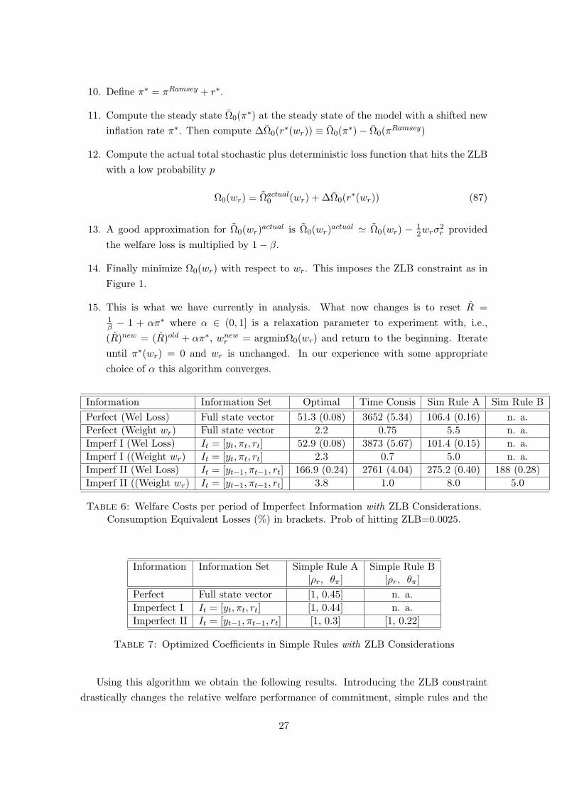
Information Information Set Optimal Time Consis Sim Rule A Sim Rule B
Perfect (Wel Loss) Full state vector 51.3 (0.08) 3652 (5.34) 106.4 (0.16) n. a.
Perfect (Weight wr) Full state vector 2.2 0.75 5.5 n. a.
Imperf I (Wel Loss) It = [yt, πt, rt] 52.9 (0.08) 3873 (5.67) 101.4 (0.15) n. a.
Imperf I ((Weight wr) It = [yt, πt, rt] 2.3 0.7 5.0 n. a.
Imperf II (Wel Loss) It = [yt−1, πt−1, rt] 166.9 (0.24) 2761 (4.04) 275.2 (0.40) 188 (0.28)
Imperf II ((Weight wr) It = [yt−1, πt−1, rt] 3.8 1.0 8.0 5.0
Table 6: Welfare Costs per period of Imperfect Information with ZLB Considerations.Consumption Equivalent Losses (%) in brackets. Prob of hitting ZLB=0.0025.
Information Information Set Simple Rule A Simple Rule B[ρr, θπ] [ρr, θπ]
Perfect Full state vector [1, 0.45] n. a.
Imperfect I It = [yt, πt, rt] [1, 0.44] n. a.
Imperfect II It = [yt−1, πt−1, rt] [1, 0.3] [1, 0.22]
Table 7: Optimized Coefficients in Simple Rules with ZLB Considerations
Using this algorithm we obtain the following results. Introducing the ZLB constraint
drastically changes the relative welfare performance of commitment, simple rules and the
27

0.3 0.4 0.5 0.6 0.7 0.8 0.9 1
1.2
1.3
1.4
1.5
1.6
1.7
1.8
1.9
2
Weight
Non−zero steady state inflation and steady state variance of interest rate
π*
σr
0.2 0.3 0.4 0.5 0.6 0.7 0.8 0.9 10
500
1000
1500
2000
2500
3000
3500
4000
4500
Weight
Loss
fuct
ion
Minimum loss and optimum weight
WelLossTotal
WelLossDeterministic
WelLossStochastic
Figure 2: Imposition of ZLB for Discretion and Perfect Information
28
withdrawal of information. Now there are substantial gains from commitment of 4 − 5%
consumption equivalent. Simple rules are less able to mimic their optimal counterpart and
the loss of information can impose a welfare loss of up to 0.24% consumption equivalent.
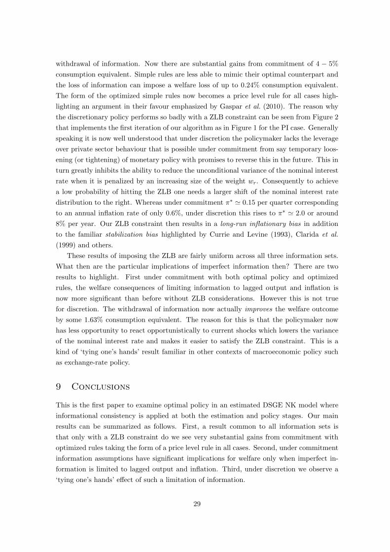
The form of the optimized simple rules now becomes a price level rule for all cases high-
lighting an argument in their favour emphasized by Gaspar et al. (2010). The reason why
the discretionary policy performs so badly with a ZLB constraint can be seen from Figure 2
that implements the first iteration of our algorithm as in Figure 1 for the PI case. Generally
speaking it is now well understood that under discretion the policymaker lacks the leverage
over private sector behaviour that is possible under commitment from say temporary loos-
ening (or tightening) of monetary policy with promises to reverse this in the future. This in
turn greatly inhibits the ability to reduce the unconditional variance of the nominal interest
rate when it is penalized by an increasing size of the weight wr. Consequently to achieve
a low probability of hitting the ZLB one needs a larger shift of the nominal interest rate
distribution to the right. Whereas under commitment π∗ ≃ 0.15 per quarter corresponding
to an annual inflation rate of only 0.6%, under discretion this rises to π∗ ≃ 2.0 or around
8% per year. Our ZLB constraint then results in a long-run inflationary bias in addition
to the familiar stabilization bias highlighted by Currie and Levine (1993), Clarida et al.
(1999) and others.
These results of imposing the ZLB are fairly uniform across all three information sets.
What then are the particular implications of imperfect information then? There are two
results to highlight. First under commitment with both optimal policy and optimized
rules, the welfare consequences of limiting information to lagged output and inflation is
now more significant than before without ZLB considerations. However this is not true
for discretion. The withdrawal of information now actually improves the welfare outcome
by some 1.63% consumption equivalent. The reason for this is that the policymaker now
has less opportunity to react opportunistically to current shocks which lowers the variance
of the nominal interest rate and makes it easier to satisfy the ZLB constraint. This is a
kind of ‘tying one’s hands’ result familiar in other contexts of macroeconomic policy such
as exchange-rate policy.
9 Conclusions
This is the first paper to examine optimal policy in an estimated DSGE NK model where
informational consistency is applied at both the estimation and policy stages. Our main
results can be summarized as follows. First, a result common to all information sets is
that only with a ZLB constraint do we see very substantial gains from commitment with
optimized rules taking the form of a price level rule in all cases. Second, under commitment
information assumptions have significant implications for welfare only when imperfect in-
formation is limited to lagged output and inflation. Third, under discretion we observe a
‘tying one’s hands’ effect of such a limitation of information.
29

There are a number of areas for future research. Our model is very basic with low
costs of business cycle fluctuations in the absence of ZLB considerations. If anything we
underestimate the costs of imperfect information. It seems therefore worthwhile to revisit
the issues raised in the context of a richer DSGE model that includes capital, sticky wages,
search-match labour market frictions and financial friction is now the subject of current
research. A second avenue for research extend the work to allow the policymaker to have
more information than the private sector. This satisfies the ICP and would allow the proper
examination of the benefits or otherwise of transparency. Finally we assume rational (model
consistent) expectations. It would be of interest to combine some aspects of learning (for
example about the policy rule) alongside model consistent expectations with imperfect as
in Ellison and Pearlman (2008).
References
Adam, K. (2007). Optimal Monetary Policy with Imperfect Common Knowledge . Journal
of Monetary Economics, 54(2), 267–301.
Adam, K. and Billi, R. M. (2007). Discretionary Monetary Policy and the Zero Lower
Bound on Nominal Interest Rates. Journal of Monetary Economics. Forthcoming.
Aoki, K. (2003). On the optimal monetary policy response to noisy indicators. Journal of
Monetary Economics, 113(3), 501 – 523.
Aoki, K. (2006). Optimal commitment policy under noisy information. Journal of Economic
Dynamics and Control, 30(1), 81 – 109.
Aoki, M. (1987). State Space Modelling of Time Series. Springer-Verlag.
Ascari, G. and Ropele, T. (2007a). Optimal Monetary Policy under Low Trend Inflation.
Journal of Monetary Economics, 54(8), 2568–2583.
Ascari, G. and Ropele, T. (2007b). Trend Inflation, Taylor Principle and Indeterminacy.
Kiel Working Paper 1332.
Blanchard, O. and Kahn, C. (1980). The Solution of Linear Difference Models under
Rational Expectations. Econometrica, 48, 1305–1313.
Blanchard, O., Giovanni, D., and Mauro, P. (2010). Rethinking Macroeconomic Policy.
IMF Staff Position Note, SPN/10/03 .
Boivin, J. and Giannoni, M. (2005). DSGE Models in a Data-Rich Environment. mimeo.
Chang, Y., Gomes, J. F., and Schorfheide, F. (2002). Learning-by-Doing as a propagation
Mechanism. American Economic Review, 92(5), 1498–1520.
30
Choudhary, A., P.Levine, McAdam, P., and Welz, P. (2011). The Happiness Puzzle: Ana-
lytical Aspects of the Easterlin Paradox. Oxford Economic Papers. Forthcoming.
Christiano, L., Eichenbaum, M., and Evans, C. (2005). Nominal Rigidities and the Dynamic
Effects of a Shock to Monetary Policy. Journal of Political Economy, 113, 1–45.
Clarida, R., Galı, J., and Gertler, M. (1999). The Science of Monetary Policy: A New
Keynesian Perspective. Journal of Economic Literature, 37(4), 1661–1707.
Coenen, G. and Wieland, V. (2003). The Zero-Interest Rate Bound and the Role of the
Exchange Rate for Monetary Policy in Japan. Journal of Monetary Economics, 50,
1071–1101.
Coibion, O., Gorodnichenko, Y., and Wieland, J. (2011). The Optimal Inflation Rate in
New Keysian Models: Should Central Banks Raise their Inflation Targets in the Light of
the ZLB? Mimeo. Presented to the CEF 2011 Conference in San Francisco .
Collard, F. and Dellas, H. (2004). The New Keynesian Model with Imperfect Information
and Learning. mimeo, CNRS-GREMAQ.
Collard, F. and Dellas, H. (2006). Misperceived Money and Inflation Dynamics. mimeo,
CNRS-GREMAQ.
Collard, F., Dellas, H., and Smets, F. (2009). Imperfect Information and the Business
Cycle. Journal of Monetary Economics. Forthcoming.
Cukierman, A. and Meltzer, A. H. (1986). A theory of ambiguity, credibility and inflation
under discretion and asymmetric information. Econometrica, 54, 1099–1128.
Currie, D. and Levine, P. L. (1993). Rules, Reputation and Macroeconomic Policy Coor-
dination. Cambridge University Press.
Doan, J., Litterman, R., and Sims, C. (1984). Forecasting and Conditional Projection Using
Realistic Prior Distributions. NBER.
Easterlin, R. A. (2003). Explaining Happiness. Proceedings of the National Academy of
Sciences of the United States, 100(19), 11176–11183.
Eggertsson, G. (2006). The Deflation Bias and Committing to Being Irresponsible. Journal
of Money, Credit and Banking, 36(2), 283–322.
Eggertsson, G. and Woodford, M. (2003). The Zero Interest-Rate Bound and Optimal
Monetary Policy. Brooking Papers on Economic Activity, 1, 139–211.
Ellison, M. and Pearlman, J. G. (2008). Saddlepath Learning. Mimeo and forthcoming,
Journal of Economic Theory.
31

Evans, G. W. and Honkapohja, S. (2009). Learning and Macroeconomics. Annual Review
of Economics, 1, 421–449.
Faust, J. and Svensson, L. (2001). Transparency and credibility: monetary policy with
unobservable goals. International Economic Review, 42, 369–397.
Faust, J. and Svensson, L. (2002). The equilibrium degree of transparency and control in
monetary policy. Journal of Money, Credit and Banking, 34(2), 520–539.
Fernandez-Villaverde, J. (2009). The Econometrics of DSGE Models. CEPR Discussion
Paper No. 7159.
Fernandez-Villaverde, J., Rubio-Ramirez, J., Sargent, T., and Watson, M. W. (2007). ABC
(and Ds) of Understanding VARs. American Economic Review, 97(3), 1021–1026.
Gaspar, V., Smets, F., and Vestin, D. (2010). Is Time Ripe for Price Level Path Stability?
In P. L. Siklos, M. T. Bohl, and M. E. Wohar, editors, Challenges in central banking:
the current institutional environment and forces affecting monetary policy. Cambridge
University Press.
Gavin, W. T. and Keen, B. D. (2011). The Zero Lower Bound and the Dual Mandate.
Mimeo. Presented to the CEF 2011 Conference in San Francisco .
Gesell, S. (1934). The Natural Economic Order. Free-Economy Publishing Co., Phlip Pye,
San Antonio.
Geweke, J. (1999). Computational Experiments and Reality. University of Minnesota and
Federal Reserve Bank of Minneapolis.
Harvey, A. (1989). Forecasting Structural Time Series and the Kalman Filter. CUP.
Juillard, M. (2003). DYNARE: A Program for Solving Rational Expectations Models.
CEPREMAP.
Keynes, J. M. (1936). The General Theory of Employment, Interest and Money. Macmillan,
New York.
Layard, R. (2006). Happiness and Public Policy: A Challenge to the Profession. Economic
Journal, 116(510), C24–C33.
Levin, A., Onatski, A., Williams, J. C., and Williams, N. (2006). Monetary Policy Under
Uncertainty in Micro-Founded Macroeconomic Models. in M. Gertler and K. Rogoff
(eds.), NBER Macroeconomics Annual, 2005, pp 229–387 .
Levine, P., Pearlman, J., and Perendia, G. (2007). Estimating DSGE Models under Par-
tial Information. Department of Economics Discussion Papers 1607, Department of
Economics, University of Surrey .
32

Levine, P., Pearlman, J., and Pierse, R. (2008a). Linear-Quadratic Approximation, Effi-
ciency and Target-Implementability. Journal of Economic Dynamics and Control, 32,
3315–3349.
Levine, P., McAdam, P., and Pearlman, J. (2008b). Quantifying and Sustaining Welfare
Gains from Monetary Commitment. Journal of Monetary Economics, 55(7), 1253–1276.
Levine, P., Pearlman, J., Perendia, G., and Yang, B. (2010). Endogenous Persistence in
an Estimated DSGE Model under Imperfect Information. Presented at the 2010 Royal
Economic Society Conference, March 29 – 31, University of Surrey and Department of
Economics Discussion Papers 0310, Department of Economics, University of Surrey .
Lungu, L., Matthews, K., and Minford, A. (2008). Partial Current Information and Signal
Extraction in a Rational Expectations Macroeconomic Model: A Computational Solu-
tion. Economic Modelling, 25(2), 255–273.
Luo, Y. and Young, E. R. (2009). Rational Inattention and Aggregate Fluctuations. The
B.E. Journal of Macroeconomics, 9(1). Article 14.
Melecky, M., Rodriguez Palenzuela, D., and Soderstrom, U. (2008). Inflation Target Trans-
parency and the Macroeconomy. MPRA Paper No. 10545.
Minford, A. and Peel, D. (1983). Some Implications of Partial Information Sets in
Macroeeconomic Models Embodying Rational Expectations. Manchester School, 51,
235–249.
Pearlman, J. G. (1992). Reputational and Non-Reputational Policies with Partial Informa-
tion. Journal of Economic Dynamics and Control, 16, 339–357.
Sims, C. (2005). Rational Inattention: A Research Agenda. Deutche Bundesbank, W.P.
no. 34/2005.
Sims, C. A. (1980). Macroeconomics and Reality. Econometrica, 48, 1–48.
Smets, F. and Wouters, R. (2003). An estimated Stochastic Dynamic General Equilibrium
Model of the Euro Area. Journal of the European Economic Association, 1(5), 1123–
1175.
Smets, F. and Wouters, R. (2007). Shocks and Frictions in US business cycles: A Bayesian
DSGE approach. American Economic Review, 97(3), 586–606.
Svensson, L. E. O. and Woodford, M. (2001). Indicator variables for Optimal Policy.
Journal of Monetary Economics, 50(3), 691–720.
Svensson, L. E. O. and Woodford, M. (2003). Indicator variables for Optimal Policy under
Asymmetric Information. Journal of Economic Dynamics and Control, 28(4), 661–680.
33
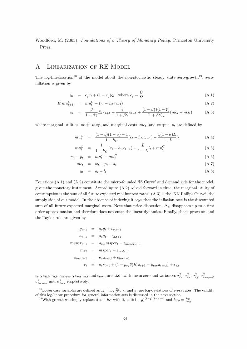
Woodford, M. (2003). Foundations of a Theory of Monetary Policy. Princeton University
Press.
A Linearization of RE Model
The log-linearization18 of the model about the non-stochastic steady state zero-growth19, zero-
inflation is given by
yt = cyct + (1− cy)gt where cy =C
Y(A.1)
EtmuCt+1 = muC
t − (rt − Etπt+1) (A.2)
πt =β
1 + βγEtπt+1 +
γ
1 + βγπt−1 +
(1− βξ)(1− ξ)
(1 + βγ)ξ(mct +mst) (A.3)
where marginal utilities, muCt , muL
t , and marginal costs, mct, and output, yt are defined by
muCt =
(1− ϱ)(1− σ)− 1
1− hC(ct − hCct−1)−
ϱ(1− σ)L
1− Llt (A.4)
muLt =
1
1− hC(ct − hCct−1) +
L
1− Llt +muC
t (A.5)
wt − pt = muLt −muC
t (A.6)
mct = wt − pt − at (A.7)
yt = at + lt (A.8)
Equations (A.1) and (A.2) constitute the micro-founded ‘IS Curve’ and demand side for the model,
given the monetary instrument. According to (A.2) solved forward in time, the marginal utility of
consumption is the sum of all future expected real interest rates. (A.3) is the ‘NK Philips Curve‘, the
supply side of our model. In the absence of indexing it says that the inflation rate is the discounted
sum of all future expected marginal costs. Note that price dispersion, ∆t, disappears up to a first
order approximation and therefore does not enter the linear dynamics. Finally, shock processes and
the Taylor rule are given by
gt+1 = ρggt + ϵg,t+1
at+1 = ρaat + ϵa,t+1
mspert+1 = ρmsmspert + ϵmsper,t+1
mst = mspert + ϵmstra,t
πtar,t+1 = ρaπtar,t + ϵtar,t+1
rt = ρrrt−1 + (1− ρr)θ(Etπt+1 − ρtarπtar,t) + ϵe,t
ϵe,t, ϵa,t, ϵg,t, ϵmsper,t, ϵmstra,t and ϵtar,t are i.i.d. with mean zero and variances σ2ϵe , σ
2ϵa , σ
2ϵg , σ
2ϵmsper
,
σ2ϵmstra
and σ2ϵtra respectively.
18Lower case variables are defined as xt = log XtX
. rt and πt are log-deviations of gross rates. The validityof this log-linear procedure for general information sets is discussed in the next section.
19With growth we simply replace β and hC with βg ≡ β(1 + g)(1−ϱ)(1−σ)−1 and hCg = hC1+g
.
34

B Priors and Posterior Estimates
Parameter Notation Prior distributionDensity Mean
Risk aversion σ Normal 1.50 0.375Price indexation γ Beta 0.50 0.15Calvo prices ξ Beta 0.50 0.10Consumption habit formation hC Beta 0.70 0.10Preference parameter ϱ Beta 0.50 0.20
Adaptive expectations
Error adjustment - Ef,tqat+1 µ1 Beta 0.50 0.20
Error adjustment - Eh,tuac,t+1 µ2 Beta 0.50 0.20
Error adjustment - Eah,t[πt+1] µ3 Beta 0.50 0.20
Proportion of rational households λh Beta 0.50 0.20Proportion of rational firms λf Beta 0.50 0.20
Interest rate rule
Inflation θπ Normal 1.50 0.25Output θy Normal 0.125 0.05Interest rate smoothing ρr Beta 0.80 0.10
AR(1) coefficient
Technology ρa Beta 0.85 0.10Government spending ρg Beta 0.85 0.10Price mark-up ρms Beta 0.50 0.20Inflation target ρtar Beta 0.85 0.10
Standard deviation of AR(1) innovations
Technology sd(ϵa) Inv. gamma 0.40 2.00Government spending sd(ϵg) Inv. gamma 1.50 2.00Price mark-up sd(ϵms) Inv. gamma 0.10 2.00Inflation target sd(ϵtar) Inv. gamma 0.10 10.00
Standard deviation of I.I.D. shocks/mearsument errors
Mark-up process sd(ϵm) Inv. gamma 0.10 2.00Monetary policy sd(ϵe) Inv. gamma 0.10 2.00Observation error (inflation) sd(ϵπ) Inv. gamma 0.10 2.00Observation error (output) sd(ϵy) Inv. gamma 0.10 2.00
Table 8: Prior Distributions
35
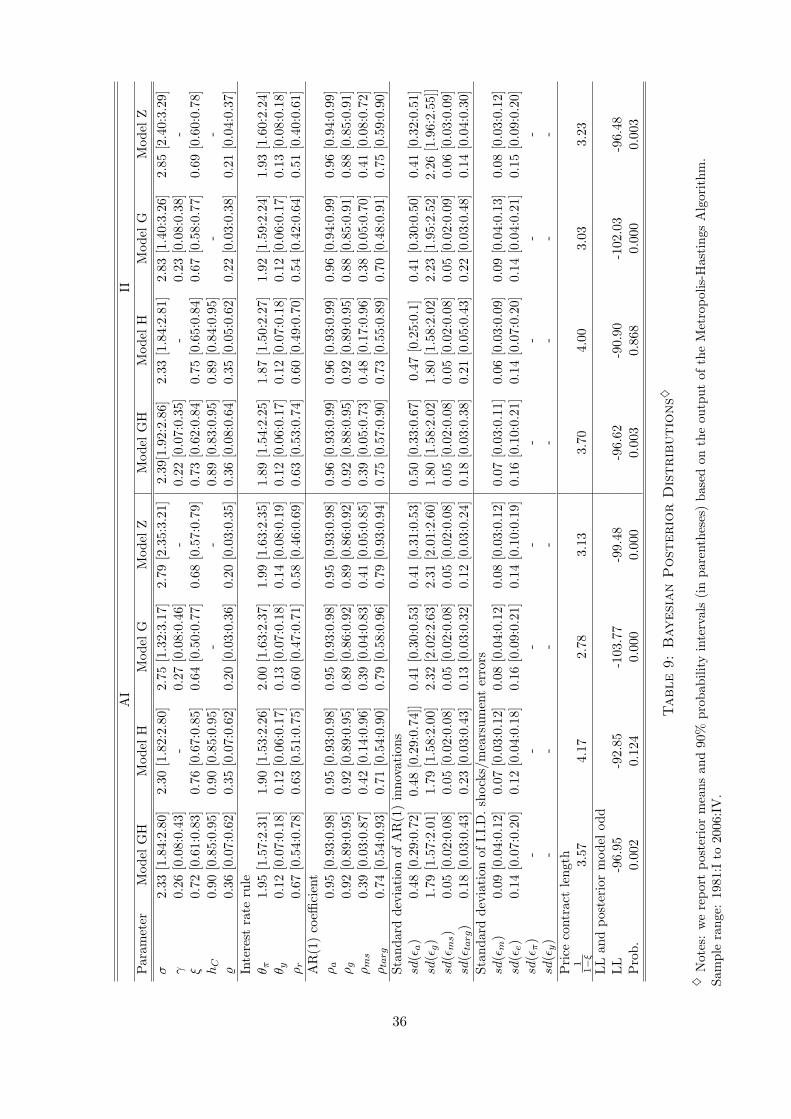
AI
II
Param
eter
Model
GH
Model
HModel
GModel
ZModel
GH
Model
HModel
GModel
Z
σ2.33[1.84:2.80
]2.30[1.82:2.80
]2.75[1.32:3.17
]2.79[2.35:3.21]
2.39[1.92
:2.86]
2.33[1.84:2.81]
2.83
[1.40:3.26
]2.85
[2.40:3.29
]γ
0.26[0.08:0.43
]-
0.27[0.08:0.46
]-
0.22[0.07:0.35
]-
0.23[0.08:0.38
]-
ξ0.72[0.61:0.83
]0.76[0.67:0.85
]0.64[0.50:0.77]
0.68[0.57:0.79]
0.73[0.62:0.84
]0.75[0.65:0.84]
0.67
[0.58:0.77
]0.69
[0.60:0.78
]hC
0.90[0.85:0.95
]0.90[0.85:0.95
]-
-0.89[0.83:0.95
]0.89[0.84:0.95]
--
ϱ0.36[0.07:0.62
]0.35
[0.07:0.62
]0.20[0.03:0.36
]0.20[0.03:0.35]
0.36[0.08:0.64
]0.35[0.05:0.62]
0.22
[0.03:0.38
]0.21
[0.04:0.37
]
Interest
rate
rule
θ π1.95[1.57:2.31
]1.90[1.53:2.26
]2.00[1.63:2.37]
1.99[1.63:2.35]
1.89[1.54:2.25
]1.87[1.50:2.27]
1.92
[1.59:2.24
]1.93
[1.60:2.24
]θ y
0.12[0.07:0.18
]0.12[0.06:0.17
]0.13[0.07:0.18
]0.14[0.08:0.19]
0.12[0.06:0.17
]0.12[0.07:0.18]
0.12
[0.06:0.17
]0.13
[0.08:0.18
]ρr
0.67[0.54:0.78
]0.63[0.51:0.75
]0.60[0.47:0.71
]0.58[0.46:0.69]
0.63[0.53:0.74
]0.60[0.49:0.70]
0.54
[0.42:0.64
]0.51
[0.40:0.61
]
AR(1)coeffi
cient
ρa
0.95[0.93:0.98
]0.95[0.93:0.98
]0.95[0.93:0.98
]0.95[0.93:0.98]
0.96[0.93:0.99
]0.96[0.93:0.99]
0.96
[0.94:0.99
]0.96
[0.94:0.99
]ρg
0.92[0.89:0.95
]0.92[0.89:0.95
]0.89[0.86:0.92
]0.89[0.86:0.92]
0.92[0.88:0.95
]0.92[0.89:0.95]
0.88
[0.85:0.91
]0.88
[0.85:0.91
]ρms
0.39[0.03:0.87
]0.42[0.14:0.96
]0.39[0.04:0.83
]0.41[0.05:0.85]
0.39[0.05:0.73
]0.48[0.17:0.96]
0.38
[0.05:0.70
]0.41
[0.08:0.72
]ρtarg
0.74[0.54:0.93
]0.71[0.54:0.90
]0.79[0.58:0.96
]0.79[0.93:0.94]
0.75[0.57:0.90
]0.73[0.55:0.89]
0.70
[0.48:0.91
]0.75
[0.59:0.90
]
Standarddeviation
ofAR(1)innovations
sd(ϵ
a)
0.48[0.29:0.72
]0.48[0.29:0.74]]
0.41
[0.30:0.53
]0.41[0.31:0.53
]0.50[0.33:0.67
]0.47
[0.25:0.1]
0.41[0.30:0.50
]0.41
[0.32:0.51
]sd(ϵ
g)
1.79[1.57:2.01
]1.79[1.58:2.00
]2.32[2.02:2.63
]2.31[2.01:2.60]
1.80[1.58:2.02
]1.80[1.58:2.02]
2.23
[1.95:2.52
]2.26
[1.96:2.55
]]sd(ϵ
ms)
0.05[0.02:0.08
]0.05[0.02:0.08
]0.05[0.02:0.08
]0.05[0.02:0.08
]0.05[0.02:0.08
]0.05[0.02:0.08]
0.05
[0.02:0.09
]0.06
[0.03:0.09
]sd(ϵ
targ)
0.18[0.03:0.43]
0.23
[0.03:0.43]
0.13
[0.03:0.32
]0.12
[0.03:0.24
]0.18[0.03:0.38
]0.21[0.05:0.43]
0.22
[0.03:0.48
]0.14
[0.04:0.30
]
Standarddeviation
ofI.I.D.shocks/mearsumenterrors
sd(ϵ
m)
0.09[0.04:0.12]
0.07[0.03:0.12]
0.08
[0.04:0.12]
0.08
[0.03:0.12]
0.07[0.03:0.11
]0.06[0.03:0.09]
0.09
[0.04:0.13
]0.08
[0.03:0.12
]sd(ϵ
e)
0.14[0.07:0.20
]0.12[0.04:0.18
]0.16[0.09:0.21
]0.14[0.10:0.19]
0.16[0.10:0.21
]0.14[0.07:0.20]
0.14
[0.04:0.21
]0.15
[0.09:0.20
]sd(ϵ
π)
--
--
--
--
sd(ϵ
y)
--
--
--
--
Price
contractlength
11−ξ
3.57
4.17
2.78
3.13
3.70
4.00
3.03
3.23
LLan
dposterior
model
odd
LL
-96.95
-92.85
-103.77
-99.48
-96.62
-90.90
-102
.03
-96.48
Prob.
0.002
0.124
0.000
0.00
00.003
0.86
80.00
00.00
3
Table9:BayesianPost
eriorDistributions
Notes:wereportposterior
meansan
d90
%probab
ilityintervals(inparentheses)based
ontheou
tputof
theMetropolis-H
astingsAlgorithm.
Sam
ple
range:
1981
:Ito
2006
:IV.
36

C Optimal Policy Under Imperfect Information: Further
Details
Pearlman (1992)20 shows that optimal policy is certainty equivalent in the sense that all the rules
under imperfect information correspond to those under perfect information, but with zt,t and xt,t
replacing zt, xt. In particular, for the fully optimal rule p2t then depends only on past values
zs,s, xs,s : s < t, so that p2t = p2t,t = p2t,t−1. (76) is then derived as follows:
xt,t +Nzt,t +Npp2t = 0 xt − xt,t = A−122 A21(zt − zt,t) (C.1)
where Np = 0 for TCT and SIM, and N is dependent on which rule is in place, and the second
equation was derived earlier. After taking expectations of each of these at t− 1, it then follows that
we can write
mt −mt,t−1 = D(zt − zt,t−1) + vt + (E −D)(zt,t − zt,t−1) (C.2)
using the previous definitions of D and E. Now assume that
zt,t − zt,t−1 = J1(D(zt − zt,t−1) + vt) (C.3)
which will be verified shortly. It then follows that
mt −mt,t−1 = (I + (E −D)J1)(D(zt − zt,t−1) + vt) (C.4)
and hence the updated value zt,t using the measurement mt is given by
zt,t − zt,t−1 = PDT (DPDT + V )−1(I + (E −D)J1)−1(mt −mt,t−1)
= PDT (DPDT + V )−1(D(zt − zt,t−1) + vt) (C.5)
Finally Pearlman (1992) shows that E[(zt − zt,t)zs,s] = 0, s ≤ t. This enables us to rewrite the
welfare loss in the form of (78), and to obtain its value in (81) using (79).
20This paper conducts the analysis in continuous time, but it is straightforward to translate the resultsand proofs to discrete time.
37