implementation of an intelligent adaptive controller...
TRANSCRIPT

International Journal of Advanced Robotic Systems Implementation of an Intelligent Adaptive Controller for an Electrohydraulic Servo System Based on a Brain Mechanism of Emotional Learning Regular Paper
Ali Sadeghieh1,*, Jafar Roshanian1 and Farid Najafi2 1 Aerospace Engineering Faculty, K.N. Toosi University of Technology, Iran 2 Mechanical Engineering Faculty, K.N. Toosi University of Technology, Iran * Corresponding author E-mail: [email protected] Received 21 Dec 2011; Accepted 04 May 2012 DOI: 10.5772/51841 © 2012 Sadeghieh et al.; licensee InTech. This is an open access article distributed under the terms of the Creative Commons Attribution License (http://creativecommons.org/licenses/by/2.0), which permits unrestricted use, distribution, and reproduction in any medium, provided the original work is properly cited.
Abstract In this paper, an experimental analysis of identification and an online intelligent adaptive position tracking control based on an emotional learning model of the human brain (BELBIC) for an electrohydraulic servo (EHS) system is presented. A mathematical model of the system is derived and the parameters of the model are identified. The BELBIC is designed based upon this dynamic model and utilized to control the real laboratorial EHS system. The experimental results are compared to those obtained from an optimal PID controller to prove that classic linear controllers fail to achieve good tracking of the desired output, especially when the hydraulic actuator operates at various frequencies and pressures. The results demonstrate an excellent improvement in control action, without any increase in control effort, for the proposed approach. Finally, it can be concluded from the experimental results that the BELBIC is able to respond quickly to any disturbance and variation in the system parameters,
showing a high degree of adaptability and robustness due to its online learning ability. Keywords Electrohydraulic servo systems, Artificial emotion, Intelligent‐adaptive systems, Nonlinear control, Real‐time implementation, System identification
Nomenclature Ai Amygdala nodal output. Av Valve orifice opening area (m2). Bv Viscous damping coefficient (N. m. sec). Cd Discharge coefficient. CL Leakage coefficient (m4. sec/kg). Dm Actuator displacement (m3/rad). E BEL model overall output. Eʹ BEL model overall output
(except Thalamus signal).
1Ali Sadeghieh, Jafar Roshanian and Farid Najafi: Implementation of an Intelligent Adaptive Controller for an Electrohydraulic Servo System Based on a Brain Mechanism of Emotional Learning
www.intechopen.com
ARTICLE
www.intechopen.com Int J Adv Robotic Sy, 2012, Vol. 9, 84:2012

eθ Position reference error (rad). Jm Actuator and load inertia (kg.m2). Kv Servo valve constant gain (m2/Volt). Oi Orbitofrontal cortex nodal output. Pc1, c2 Pressure in the actuator chambers (Pa). PL Load pressure (Pa). Ps Supply pressure (Pa). Qc1, c2 Flow rate in/out of the actuators (m3/sec). REW Emotional signal. Si Sensory input signal. Sth Thalamus signal. t Time (sec). u Servo valve control input (Volt). Vi Amygdala adaptive gain for node i. Vt Oil volume under compression (m3). Wi Orbitofrontal cortex adaptive
gain for node i. yp Plant output (rad). yr Reference output (rad). αa Amygdala learning rate. αo Orbitofrontal cortex learning rate. β Fluid bulk modulus (Pa). ρ Fluid mass density (kg/m3). θ Actuator angular position (rad). τv Servo valve time constant (sec).
1. Introduction Recently, electrohydraulic servo (EHS) systems have become increasingly popular in many types of industrial equipment and processes. EHS systems have been used in industry for a wide range of applications due to their small size to power ratio and their ability to apply a very large force and control accuracy. Instances of the applications of these systems may be found in the control of industrial robots, the machine tool industry, milling machines, automobiles, punching presses, material testing equipment, aerospace industries, and the like. However, the dynamics of hydraulic systems are highly nonlinear; the system may be subject to non‐smooth nonlinearities due to control input saturation, the directional change of valve opening, friction and valve overlap; laminar and turbulent flows, channel geometry and friction result in system equations that are highly nonlinear. The parameters of such hydraulic systems, depending on the relation between flow velocity, pressure and oil viscosity, vary heavily. Aside from the nonlinear nature of hydraulic dynamics, electrohydraulic servo systems also have many model uncertainties [1], such as external disturbances and leakages that cannot be modelled exactly of which the nonlinear functions that describe them may not be known. While an accurate modelling involving all the nonlinearities is helpful in the
description of such complex dynamic behaviour, it complicates the hydraulic system model for identification and control strategy. Much research has been conducted on the control of servo hydraulic systems. In early studies, linear models around working points and linear control strategies were applied [2]. Although linear control methods work well for some systems, for highly nonlinear systems with time varying dynamics (such as EHS systems) they may not ensure acceptable control performance. To improve control system behaviour for nonlinear time variant systems ‐ such as EHS systems ‐ robust and adaptive controllers have been applied in those systems [3], [4]. However, the controller is based on a linear model of the plant, which imposes certain limitations on the efficiency and robustness of the controller. Nonlinear control strategies such as sliding mode [5], [6], feedback linearization [7] or backstepping [8] approaches depict more satisfactory results but they require a more accurate model of the system. Besides this, the controller design and experimental implementation of these controllers are somewhat complicated. Recently, intelligent control has been widely considered due to its high flexibility in relation to feedbacks and the selection of control parameters and its low dependency on the accuracy of a dynamic model. Model‐based approaches to decision‐making are being replaced by data‐driven and rule‐based approaches in recent years. One of the most popular of these approaches is fuzzy set theory. Fuzzy control [9], [10], in using linguistic information, possesses several advantages such as its being model‐free, its robustness, its universal approximation theorem and its rule‐based algorithm. However, the huge number of fuzzy rules for high‐order systems makes the analysis complex. New approaches, in which intelligence is not given to the system from outside but is acquired by the system through learning, have proven much more successful [11]. Because of their self‐learning, self‐organizing and self‐adapting capability, neural networks have become a powerful tool for many complex applications, such as EHS systems [12], [13]. However neural network controllers require a predefined structure which may lead to additional time consuming computations during the control process. The other drawback of neural network controllers is their output dependency on the selection of the initial values of the neural network weights. The successful adoption and, therefore, implementation [14]‐[19] of a neuro‐computing model for the intelligent‐adaptive control of dynamic systems investigated by Lucas et al. [20] based on a simple but effective computational model of an emotional learning scheme in
2 Int J Adv Robotic Sy, 2012, Vol. 9, 84:2012 www.intechopen.com
the amygdala as introduced recently by Moren and Balkenius [21] motivated us for the further study of this scheme. The model introduced by Moren and Balkenius aims to partly regenerate the same characteristics of the biological system by presenting a neurologically inspired computational model of the amygdala and the orbitofrontal cortex (OFC). In the leading research carried out by Lucas et al., a simplified version of a previously developed emotional learning model of the amygdala [21] was employed in order to present an adaptive control strategy, designated as a Brain Emotional Learning Based Intelligent Controller (BELBIC). A BELBIC possesses several important features such as online adaptation, learning ability, a straight‐forward control system architecture and low online computational load. The recently modified version of a BELBIC introduced in this paper works exactly like the model of emotional learning in human brain and mimics the amygdala, the OFC, the thalamus, and the Sensory input cortex. This BELBICs is known to be suitable for the online direct‐adaptive‐control of nonlinear dynamic systems [22] and it has shown its abilities in this research by being implemented for the design of a positioning control of a nonlinear electrohydraulic servo system. This paper is organized as follows. First, the structure of the novel emotional controller is presented in Section 2. The details of the design process of the BELBIC controller are given at the end of the paper in the Appendix. Next, Section 3 explains a complete description of the mathematical model used. Section 4 deals with the identification algorithm of the system parameters. Section 5 contains a brief description of the electrohydraulic workbench used to implement the real‐time work. In Section 6, the presentation of the identification results is followed by the comparison of the experimental results obtained from applying the BELBIC to a real plant with those of a real‐time PID controller. Finally, some conclusions and remarks bring this work to a close in Section 7. 2. BELBIC 2.1 Computational model of the Brain Emotional Learning (BEL) mechanism The most important aspect of any intelligent system is its capability to learn, e.g., supervised learning (where the algorithm generates a function that maps inputs to desired outputs), unsupervised learning (which models a set of inputs ‐ labelled examples are not available) and reinforcement learning (where the algorithm learns a policy of how to act given an observation of the world).
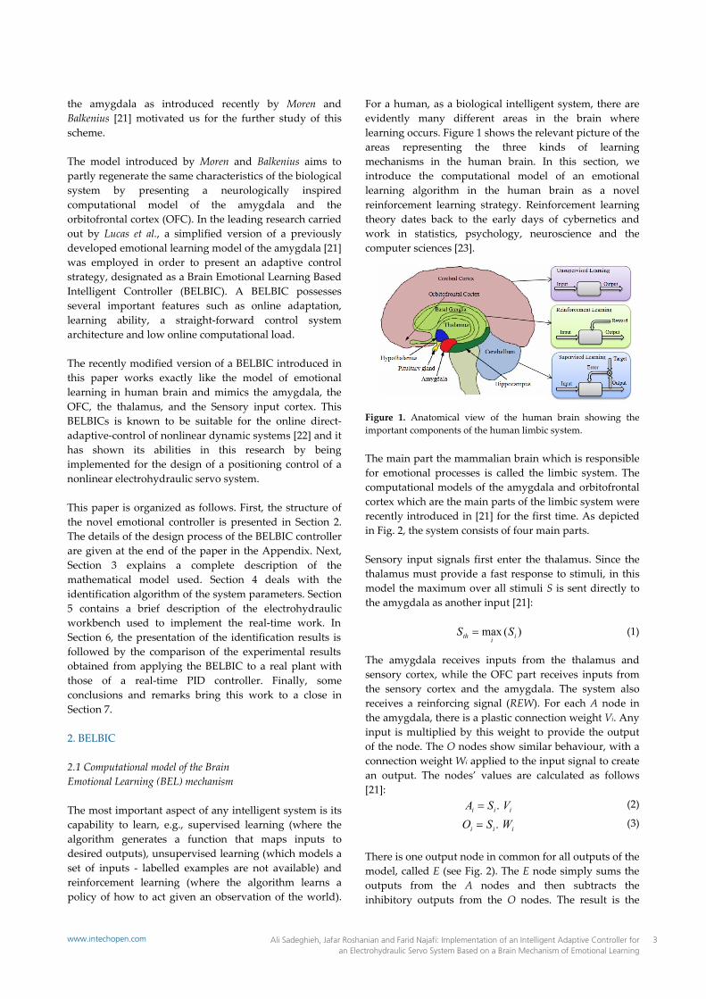
For a human, as a biological intelligent system, there are evidently many different areas in the brain where learning occurs. Figure 1 shows the relevant picture of the areas representing the three kinds of learning mechanisms in the human brain. In this section, we introduce the computational model of an emotional learning algorithm in the human brain as a novel reinforcement learning strategy. Reinforcement learning theory dates back to the early days of cybernetics and work in statistics, psychology, neuroscience and the computer sciences [23].
Figure 1. Anatomical view of the human brain showing the important components of the human limbic system. The main part the mammalian brain which is responsible for emotional processes is called the limbic system. The computational models of the amygdala and orbitofrontal cortex which are the main parts of the limbic system were recently introduced in [21] for the first time. As depicted in Fig. 2, the system consists of four main parts. Sensory input signals first enter the thalamus. Since the thalamus must provide a fast response to stimuli, in this model the maximum over all stimuli S is sent directly to the amygdala as another input [21]:
The amygdala receives inputs from the thalamus and sensory cortex, while the OFC part receives inputs from the sensory cortex and the amygdala. The system also receives a reinforcing signal (REW). For each A node in the amygdala, there is a plastic connection weight Vi. Any input is multiplied by this weight to provide the output of the node. The O nodes show similar behaviour, with a connection weight Wi applied to the input signal to create an output. The nodes’ values are calculated as follows [21]:
(2) iii VSA . (3) iii WSO .
There is one output node in common for all outputs of the model, called E (see Fig. 2). The E node simply sums the outputs from the A nodes and then subtracts the inhibitory outputs from the O nodes. The result is the
(1) )(max iith SS
3Ali Sadeghieh, Jafar Roshanian and Farid Najafi: Implementation of an Intelligent Adaptive Controller for an Electrohydraulic Servo System Based on a Brain Mechanism of Emotional Learning
www.intechopen.com

output from the model. The Eʹ node sums the outputs from A except for the Ath and then subtracts the inhibitory outputs from the O nodes.
( including Sth) (4) ii OAE (except Sth) (5) ii OAE
Figure 2. A Graphical depiction of the brain emotional learning process [21]. Emotional learning occurs mainly in the amygdala. The learning rule of the amygdala is given as follows:
(6)
jjiai AREWSV ,0max
where αa is the amygdala learning rate that is constant and REW is the reinforcing signal. The term max is to make the learning changes monotonic, implying that the amygdala’s gain can never be decreased. This rule is for modelling the incapability of unlearning the emotion signal (and consequently, emotional action) previously learned in the amygdala. Similarly, the learning rule in the orbitofrontal cortex is shown as:
(7) REWESW ioi
where αo is the learning rate constant in the OFC. The orbitofrontal learning rule is very similar to the amygdala rule. The only difference is that the OFC connection weight can either increase or decrease as needed to track the required inhibition, which is reflected as the discrepancy between the reinforcing signal (REW) and the Eʹ node. The system operation consists of two levels: the amygdala learns to predict and react to a given reinforcement signal. This subsystem cannot unlearn a connection. The
incompatibility between predictions and the actual reinforcement signals causes inappropriate responses from the amygdala. The OFC learns to prevent the system output if such mismatches occur. The learning in the amygdala and the OFC is performed by updating the plastic connection weights, based on the received reinforcing and stimulus signals. 2.2 Brain Emotional Learning Based Intelligent Controller (BELBIC) structure In a biological system, emotional reactions are utilized for fast decision‐making in complex environments or emergency situations. It is thought that the amygdala and the orbitofrontal cortex are the most important parts of the brain involved in emotional reactions and learning [24]. The amygdala is a small structure in the medial temporal lobe of the brain that is thought to be responsible for the emotional evaluation of stimuli [25]. This evaluation is in turn used as a basis for emotional states and reactions and is used for attention signals and laying down long‐term memories [25]. The amygdala and the orbitofrontal cortex compute their outputs based on the emotional signal (the reinforcing signal) received from the environment. The final output (the emotional reaction) is calculated by subtracting the amygdala’s output from the orbitofrontal cortex’s output (see Fig. 3). To use our version of the Moren‐Balkenius model as a controller, it should be observed that it essentially converts two sets of inputs (sensory inputs and emotional cues or reinforcing signals) into the decision signal (the emotional reaction) as its output. Closed loop configurations using this block (BELBIC) in the feed‐forward‐loop of the total system in an appropriate manner have been implemented so that the input signals have the proper interpretations. The block implicitly implemented the critic, the learning algorithm and the action selection mechanism used in the functional implementations of emotionally‐based (or, generally, reinforcement learning‐based) controllers, all at the same time.
Figure 3. The process of generating emotional reactions in the limbic part of the human brain.
4 Int J Adv Robotic Sy, 2012, Vol. 9, 84:2012 www.intechopen.com
In the implementation of the BELBIC, it should be pointed out that since this model has originally been proposed for descriptive purposes with no control engineering motivation, the model is essentially an open loop. To be used as a controller, the designer has to choose the sensory input fed back from the system response as well as the reward function, in accordance with the control engineering requirements of the problem at hand and not merely from neurocognitive insights. The design of the BELBIC is, therefore, no different from the design of any other nonlinear or adaptive control schemes [26]. The reinforcing signal (REW) comes as a function of the other signals which can be supposed as a cost function validation. Specifically, a reward (or punishment) is applied based on a previously defined cost function:
(8) ),,( ueSJREW i
The choice of external reinforcement signal provides a degree of freedom for multi‐objective learning procedures. Similarly, the sensory inputs can be a function of plant and controller outputs, as follows:
(9) ),,,( rp yyeufS
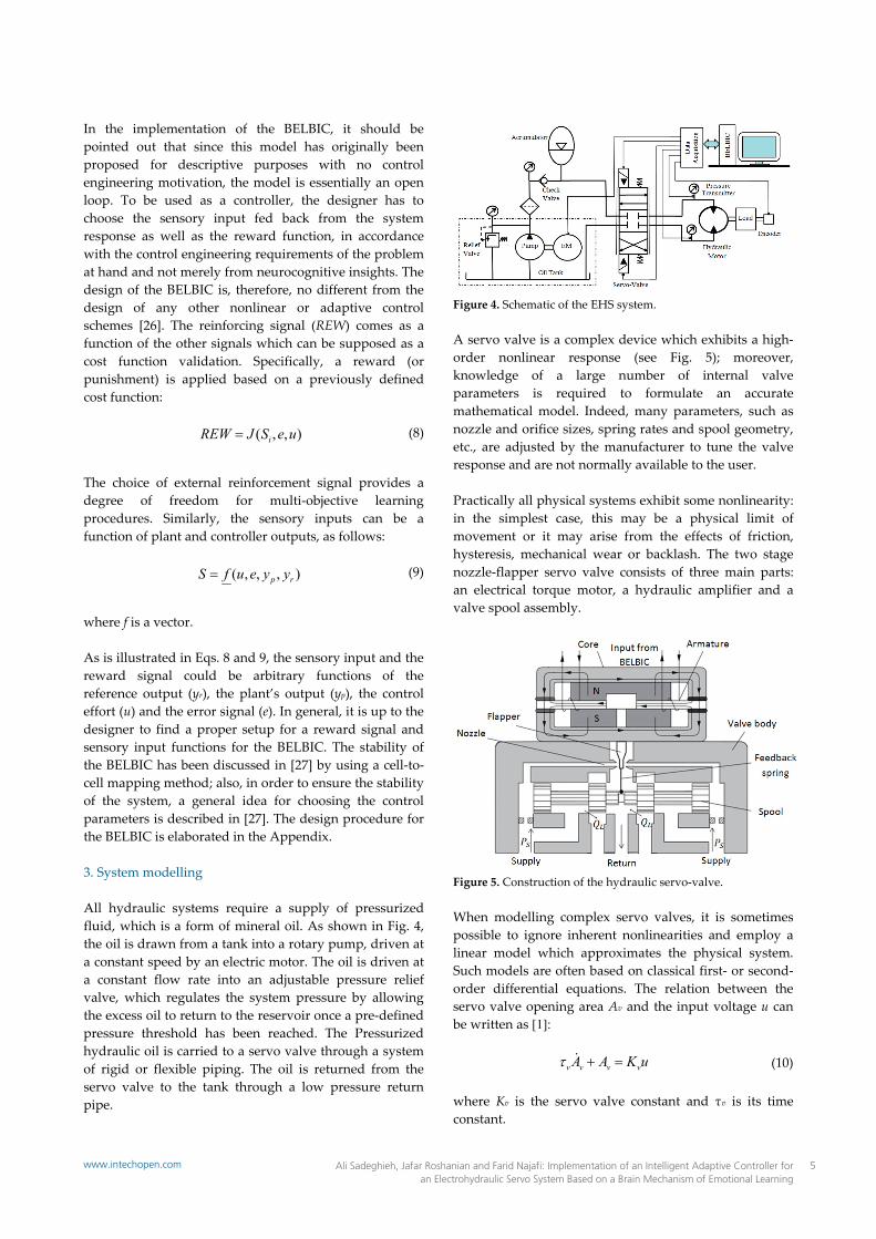
where f is a vector. As is illustrated in Eqs. 8 and 9, the sensory input and the reward signal could be arbitrary functions of the reference output (yr), the plant’s output (yp), the control effort (u) and the error signal (e). In general, it is up to the designer to find a proper setup for a reward signal and sensory input functions for the BELBIC. The stability of the BELBIC has been discussed in [27] by using a cell‐to‐cell mapping method; also, in order to ensure the stability of the system, a general idea for choosing the control parameters is described in [27]. The design procedure for the BELBIC is elaborated in the Appendix. 3. System modelling All hydraulic systems require a supply of pressurized fluid, which is a form of mineral oil. As shown in Fig. 4, the oil is drawn from a tank into a rotary pump, driven at a constant speed by an electric motor. The oil is driven at a constant flow rate into an adjustable pressure relief valve, which regulates the system pressure by allowing the excess oil to return to the reservoir once a pre‐defined pressure threshold has been reached. The Pressurized hydraulic oil is carried to a servo valve through a system of rigid or flexible piping. The oil is returned from the servo valve to the tank through a low pressure return pipe.
Figure 4. Schematic of the EHS system. A servo valve is a complex device which exhibits a high‐order nonlinear response (see Fig. 5); moreover, knowledge of a large number of internal valve parameters is required to formulate an accurate mathematical model. Indeed, many parameters, such as nozzle and orifice sizes, spring rates and spool geometry, etc., are adjusted by the manufacturer to tune the valve response and are not normally available to the user. Practically all physical systems exhibit some nonlinearity: in the simplest case, this may be a physical limit of movement or it may arise from the effects of friction, hysteresis, mechanical wear or backlash. The two stage nozzle‐flapper servo valve consists of three main parts: an electrical torque motor, a hydraulic amplifier and a valve spool assembly.
Figure 5. Construction of the hydraulic servo‐valve. When modelling complex servo valves, it is sometimes possible to ignore inherent nonlinearities and employ a linear model which approximates the physical system. Such models are often based on classical first‐ or second‐order differential equations. The relation between the servo valve opening area Av and the input voltage u can be written as [1]:
(10) uKAA vvvv where Kv is the servo valve constant and τv is its time constant.
5Ali Sadeghieh, Jafar Roshanian and Farid Najafi: Implementation of an Intelligent Adaptive Controller for an Electrohydraulic Servo System Based on a Brain Mechanism of Emotional Learning
www.intechopen.com

Defining the supply pressure Ps as Ps=Pc1+Pc2, the load pressure PL as PL=Pc1–Pc2 and the load flow QL as QL=(Qc1+ Qc2)/2, the relationship between the load pressure PL and the load flow QL for an ideal critical centre servo valve with a matched and symmetric orifice, assuming a small leakage, it can be expressed as follows [1]:
(11)
)( vLSvdL
AsignPPACQ
where Cd is the flow discharge coefficient and ρ is the fluid mass density. The sign function in Eq. 11 stands for the change in the direction of fluid flow through the servo valve. When the continuity equation is applied to the fluid flowing in the actuator dynamics along with the oil leakage, the following expression can be derived:
(12) LLmvLS
vdLt PCDAsignPPACPV
)(2
where CL is the total leakage coefficient of the motor, β is the fluid bulk modulus, θ is the output angular position, Vt is the total volume of the servo valve and the actuator, and Dm is the actuator volumetric displacement. Neglecting Coulomb frictional torque, the motion equation of the hydraulic actuator is given by:
(13) dtdJBPPD mvCCm )( 21
where Bv is the viscous damping coefficient and Jm is total inertia of the motor and load referred to by the motor shaft. Finally, if the state variables are denoted by: x1‐ hydro motor angular position (rad), x2‐ hydro motor angular velocity (rad/sec), and x3‐ load pressure differential (Pa), the system can be easily described with a third‐order nonlinear state‐space model:
(14)
2332313
22312
21
)( xpxpAsignxPApx
xwxwxxx
vSv
where the valve area opening (Av) can be determined from Eq. 10 and w1, w2, p1, p2 and p3 are appropriate constants given by:
(15) m
v
m
m
JBw
JDw 21 ,
.2,2,2321
t
m
t
L
t
d
VDp
VCp
VCp
In this first step, the mathematical model of the electrohydraulic system was fully designed and established. The next step involves setting up an identification algorithm for the system parameters. 4. System identification algorithm In the system model (Eq. 14), it can be seen that the parameters to be identified are those in the last two equations. Therefore, only parameters w1, w2, p1, p2 and p3 need to be identified in the following equations:
(16)
2332313
22312
)( xpxpAsignxPApx
xwxwx
vSv
Equation 16 can be rewritten in matrix form as:
(17)
3
2
1
2
1
233
23
3
2
)(00000
pppww
xxAsignxPAxx
xx
vSv
It can be seen that the system (Eq. 17) has linear parameters, which is a sufficient condition for those parameters to be identified through the continuous recursive least square method with a constant trace [28]. Now let:
(18)
,)(3
2
xx
ty
,)(00
000)(
233
23
xxAsignxPAxx
tvSv
T
.)(
3
2
1
2
1
pppww
t
Then:
(19) Ttty )()(
where y is the observed vector of variables, φ is the matrix of regression variables and θ is the vector of unknown parameters. The parameter should be determined so that the criterion:
(20) dsssyeVt Tts
0
2
is minimized. For parameter α, α ≥ 0 corresponds to the forgetting factor. A straightforward calculation shows that the criterion is minimized if:
6 Int J Adv Robotic Sy, 2012, Vol. 9, 84:2012 www.intechopen.com

(21)
dedssset
Ttt
Tts
00
ˆ
which is the normal equation. The estimate is unique if the matrix:
(22)
dsssetR
tTts
0
is invertible. Finally, assuming that matrix P(t)=R(t)‐1, the parameter estimate that minimizes the least square error must satisfy:
(23)
)()()()()()()(ˆ)()()(
)()()()(ˆ
tPtttPtPdttdP
tttyte
tettPdttd
T
T
Through Eq. 23, we can now identify the system parameters in Eq. 15 and, consequently, begin the design of the BELBIC controller. 5. Experimental workbench and settings
Figure 6. Experimental EHS system workbench: 1—electric motor; 2—pump; 3—accumulator; 4—relief valve; 5—tank; 6— rotary hydraulic actuator; 7—two stage servo valve; 8—load; 9—interface card; 10—encoder; 11—pressure sensors; 12—electric power supply; and 13—pressure transmitter. In order to analyse the performance of the identification and controller, experimental tests have been carried out. The experimental test rig is shown in Fig. 6. All of the programs for the system were developed using the MATLAB‐Simulink software and C S‐Function blocks. The command signal from the computer was sent to a
servo valve driver by a 12‐bit interface card. The sampling time for the experimental implementation of the proposed EHS system with the emotional controller is determined as 1ms. The angular position of the hydro motor shaft is measured via an encoder which is mounted at the motor shaft end. The maximum working pressure, during all of the experiments, is set at 110 bars, which is the pressure threshold for the relief valve to open. 6. Experimental results and discussion This section presents and analyses the experimental results obtained from the BELBIC controller versus those obtained from a real‐time PID controller, since the PID is the most popular and widespread controller used in industry. We therefore held it as a reference for the sake of comparison. The goal is to evaluate the system transient response, the steady state behaviour, the magnitude and the uniformity of the control signal. 6.1 Identification The online identification of the system parameters is based on the recursive least square algorithm with a constant trace. The identification procedure is achieved in an open‐loop system. In fact, the input signal that is sent to the servo valve is a sine wave with an 8 rad/sec frequency and a 0.1 Volt amplitude, plus a low power white noise with a variance of 0.002 added to include all of the frequencies. During identification, the sampling time was set to 1ms. The intensity of the input noise is set so as to be effective on the states of the system. Since the data acquired from the sensors ‐ especially the pressure sensors ‐ is always noisy, the appropriate filters should be used to reduce the noise. The type, order and other details of the filters are determined by trial‐and‐error. An important fact in filter selection is that the designed filter must be able to decrease environmental noises but not totally eliminate the effect of input noise. A first‐order low pass Butterworth filter with a pass band frequency of 50 rad/sec is applied. After 6 seconds of identification, the system parameters became fairly constant and were set at the following values in Table 1 in order to design the BELBIC controller parameters: parameter value unit
w1 4.2×10‐5 kgm /
w2 7.1 sec/1
p1 2.9×10¹⁰ )sec./( 22/52/1 mkg
p2 0.4 sec/1
p3 8.5×10⁶ )sec./( 2mkg
Table 1. Identification results of the EHS system parameters
7Ali Sadeghieh, Jafar Roshanian and Farid Najafi: Implementation of an Intelligent Adaptive Controller for an Electrohydraulic Servo System Based on a Brain Mechanism of Emotional Learning
www.intechopen.com
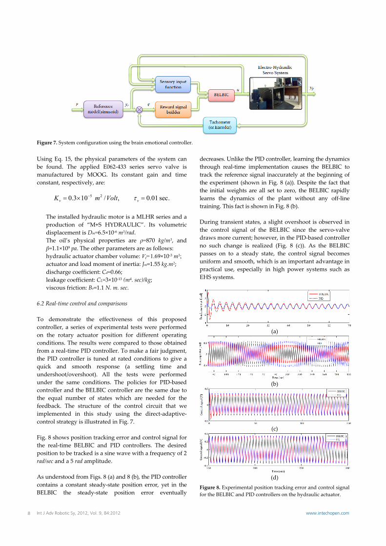
Figure 7. System configuration using the brain emotional controller. Using Eq. 15, the physical parameters of the system can be found. The applied E062‐433 series servo valve is manufactured by MOOG. Its constant gain and time constant, respectively, are:
.sec01.0,/103.0 25 vv VoltmK
The installed hydraulic motor is a MLHR series and a production of “M+S HYDRAULIC”. Its volumetric displacement is Dm=6.5×10‐6 m3/rad. The oil’s physical properties are ρ=870 kg/m3, and β=1.1×10⁹ pa. The other parameters are as follows: hydraulic actuator chamber volume: Vt=1.69×10‐3 m3; actuator and load moment of inertia: Jm=1.55 kg.m2; discharge coefficient: Cd=0.66; leakage coefficient: CL=3×10‐13 (m4. sec)/kg; viscous friction: Bv=1.1 N. m. sec.
6.2 Real‐time control and comparisons To demonstrate the effectiveness of this proposed controller, a series of experimental tests were performed on the rotary actuator position for different operating conditions. The results were compared to those obtained from a real‐time PID controller. To make a fair judgment, the PID controller is tuned at rated conditions to give a quick and smooth response (a settling time and undershoot/overshoot). All the tests were performed under the same conditions. The policies for PID‐based controller and the BELBIC controller are the same due to the equal number of states which are needed for the feedback. The structure of the control circuit that we implemented in this study using the direct‐adaptive‐control strategy is illustrated in Fig. 7. Fig. 8 shows position tracking error and control signal for the real‐time BELBIC and PID controllers. The desired position to be tracked is a sine wave with a frequency of 2 rad/sec and a 5 rad amplitude. As understood from Figs. 8 (a) and 8 (b), the PID controller contains a constant steady‐state position error, yet in the BELBIC the steady‐state position error eventually
decreases. Unlike the PID controller, learning the dynamics through real‐time implementation causes the BELBIC to track the reference signal inaccurately at the beginning of the experiment (shown in Fig. 8 (a)). Despite the fact that the initial weights are all set to zero, the BELBIC rapidly learns the dynamics of the plant without any off‐line training. This fact is shown in Fig. 8 (b). During transient states, a slight overshoot is observed in the control signal of the BELBIC since the servo‐valve draws more current; however, in the PID‐based controller no such change is realized (Fig. 8 (c)). As the BELBIC passes on to a steady state, the control signal becomes uniform and smooth, which is an important advantage in practical use, especially in high power systems such as EHS systems.
(a)
(b)
(c)
(d)
Figure 8. Experimental position tracking error and control signal for the BELBIC and PID controllers on the hydraulic actuator.
8 Int J Adv Robotic Sy, 2012, Vol. 9, 84:2012 www.intechopen.com

Figure 9. Experimental position tracking error for a sudden increase in frequency (from 2 to 4 rad/sec): (a) BELBIC controller, and (b) PID controller. Another experiment was carried out with a sudden increase in the frequency of the reference command position (shown in Figs. 9 and 10). The frequency is changed suddenly from 2 to 4 rad/sec just after 150 seconds. The BELBIC adapts with the alteration in the reference signal, as shown in Fig. 9(a). In time, it learns how to respond to the modified reference command, maintaining the stability of the EHS system (during the relatively long experiment period). The BELBIC tracks the reference signal with very low error in comparison with the PID controller (as shown in Fig. 9). It can be seen in Fig. 10 that the energy consumption of the BELBIC is about the same as the PID controller, whilst the BELBIC has less tracking error.
Figure 10. Experimental control signal for a sudden increase in frequency (from 2 to 4 rad/sec) for BELBIC and PID controllers.
Figure 11. Experimental position tracking error with a gradual decreasing in pressure (from 100 to 50 bars): (a) BELBIC controller, and (b) PID controller.
(a) (b)
(b) (a)
9Ali Sadeghieh, Jafar Roshanian and Farid Najafi: Implementation of an Intelligent Adaptive Controller for an Electrohydraulic Servo System Based on a Brain Mechanism of Emotional Learning
www.intechopen.com

Figure 12. Experimental control signal with a gradual decreasing in pressure (from 100 to 50 bars) for BELBIC and PID controllers. In common industrial applications, the robustness of the controller with respect to changing the operating conditions is a serious problem. To evaluate the capability of the new emotional controller in terms of handling these changes, after 150 seconds the supply pressure of the system is altered. This pressure is gradually decreased from 100 to 50 bars, which causes a change in the control signal generated by the BELBIC and the PID. As shown in Fig. 12, the control signal of the BELBIC is nearly similar to that of the PID. As concluded from Fig. 11, the BELBIC displays good robustness to a change in the dynamics of the system, an acceptable overshoot and a good tracking ability (compared to the PID). 7. Conclusion In this paper, a comprehensive investigation was carried out on the modelling, identification and control of a real laboratorial EHS system. System identification was rendered by simply rewriting the system model in an LP form, allowing the use of the recursive least square algorithm for this purpose. Then, an innovative brain emotional controller was employed for position tracking. Before experimental application, the values of the parameters of this controller were determined based on the extracted mathematical model. The performance of the emotional controller has been compared with those of the conventional PID controller, especially with respect to its adaptability to frequency and pressure variations. In the evaluation of the proposed control method, the following points have to be taken into consideration. As time passes, the BELBIC learns the dynamics of the plant, causing less tracking error than the PID controller, whilst the energy consumption of the BELBIC is similar to that of the PID controller. Another advantage of the BELBIC compared with other controllers in practical applications is in its production of a uniform and smooth control
signal. Besides, the computational burden is very light, as seen in Eqs. 1 to 9. It has been reported that the use of other advanced control techniques, while also yielding better performance than PID controllers, has had some disadvantages; unlike the BELBIC they suffer from an increase in control effort, a non‐smooth control signal, more difficult implementation and a high computational load. A main advantage in the performance of the controlled EHS system is in the high degree of the adaptability of the control system and the robustness of the performance with respect to the initial error in relation to modelling and identification (even with a total lack of knowledge about the system model). The main shortcoming of model‐free controllers with a learning ability ‐ without any prior knowledge of the system’s dynamics, such as through reinforcement learning‐based controllers and the BELBIC ‐ is that in the early phases of the learning process, they may cause poor performance because they may produce a wrong control signal. Future research can focus on a hybrid control to solve this problem and accelerate the learning phase. Undoubtedly, the proposed approach is not an optimal solution; however with simple implementation, reasonable computational effort, fast response and an insensitivity to disturbances, this method proves to be both efficient and acceptable. 8. Appendix In this section, the controller design procedure is presented in order to control the angular position of the rotary electrohydraulic servo system according to the intelligent control algorithm introduced in section 2. Consider the direct‐adaptive‐control strategy as specified in Fig. 7. It was mentioned in Section 2.2 that the BELBIC must be provided with a set of sensory input signals in addition to a reward signal. The sensory input vector selected to solve this problem consists of three signals (Eq. 24) plus a reward signal (Eq. 25). The sensory input vector opted for with the electrohydraulic servo system control weighted the feedback error signal, the reference command signal and the time integral of the commanded voltage signal as its three components. The coefficients are chosen via trial and error. The reward function (Eq. 25) is similar to a proportional‐integral control scheme seeking a suitable tradeoff between the quick adjustment of error and the long‐term elimination of steady‐state error.
(24)T
r dtuyeS
33
(25) dteeREW 15.06.0
10 Int J Adv Robotic Sy, 2012, Vol. 9, 84:2012 www.intechopen.com

The term ∫u aims to help the BELBIC to minimize its energy consumption (control effort). The learning rates in the amygdala and the OFC are set as αa=42e–5 and αo=22e–4, respectively. The art of the designer is required to cope appropriately with choosing the system’s emotional condition and tuning the learning rates of the system itself in order to obtain the desired goal. 9. Acknowledgements The authors would like to express their gratitude to the deceased Prof. Caro Lucas from the Department of Electrical and Computer Engineering, University of Tehran, for his valuable recommendations. Also, we are very thankful to the staff of the actuators and virtual reality research laboratories in the Mechanical Engineering Faculty of K.N. Toosi University of Technology. It was their genuine help and patience that made the required tests possible throughout this research process. 10. References [1] H. E. Merritt, Hydraulic Control Systems. New York:
John Wiley and Sons, 1967. [2] T. J. Lim, “Pole placement control of an electro‐
hydraulic servo motor,” in Proc. 1997 2nd Int. Conf. Power Electron. Drive Syst., Part 1, vol. 1, Singapore, May 26‐29, pp. 350–356.
[3] M. J. Plahuta, M. A. Franchek, and H. Stern, “Robust controller design for a variable displacement hydraulic motor,” in Proc. 1997 ASME Int. Mech. Eng. Congr. Expo., vol. 4, Nov. 16–21, pp. 169–176.
[4] W.‐S. Yu and T.‐S. Kuo, “Robust indirect adaptive control of the electrohydraulic velocity control systems,” in Proc. Inst. Elect. Eng.: J. Control Theory Appl., vol. 143, no. 5, Sep. 1996, pp. 448–454.
[5] A. Fink and T. Singh, “Discrete sliding mode controller for pressure control with an electrohydraulic servo valve,” in Proc. 1998 IEEE Int. Conf. Control Appl., vol. 1, Trieste, Italy, pp. 378–382.
[6] H.‐M. Chen, J.‐C. Renn and J.‐P. Su, “Sliding mode control with varying boundary layers for an electro‐hydraulic position servo system,” in Springer, Int. J. Adv. Manuf. Technol., vol. 26, 2005, pp. 117–123.
[7] H. Hahn, A. Piepenbrink and K.‐D. Leimbach, “Input/output linearization control of an electro servo‐hydraulic actuator,” in Proc. 3rd IEEE Conf. Control Appl., vol. 2, Glasgow, U. K., Aug. 1994, pp. 995–1000.
[8] C. Kaddissi, J.‐P. Kenné and M. Saad, “Identification and Real‐Time Control of an Electrohydraulic Servo System Based on Nonlinear Backstepping,” in IEEE Trans. Mechatron., vol. 12, no. 1, Feb. 2007, pp. 1083‐4435.
[9] S. Y. Lee and H. S. Cho, “A fuzzy controller for an electro‐hydraulic fin actuator using phase plane method,” in Control Eng. Practice, vol. 11, no. 6, Jun. 2003, pp. 697‐708.
[10] P. J. C. Branco and J. A. Dente, “On using fuzzy logic to integrate learning mechanisms in an electro‐hydraulic system—Part I: Actuator’s fuzzy modeling,” in IEEE Trans. Syst. Man Cybern. C,Appl. Rev., vol. 30, no. 3, 2000, pp. 305–316.
[11] M. Fatourechi, C. Lucas and A. Khaki Sedigh, “Emotional learning as a new tool for development of agent based system,” in Informatica, vol. 27, no. 2, 2003, pp. 137–144.
[12] M. Karimi, F. Najafi, H. Sadati and M. Saadat, “Application of a flexible structure artificial neural network on a servo‐hydraulic rotary actuator,” in Springer, Int. J. Adv. Manuf. Technol., vol. 39, no. 5‐6, 2008, pp. 559‐569.
[13] T. Knohl and H. Unbehauen, “Adaptive Position Control of Electrohydraulic Servo System Using ANN,” in J. Mechatron., Elsevier Sci. Ltd, vol. 10, 2000, pp. 127‐143.
[14] M. R. Jamali, A. Arami, B. Hosseini, B. Moshiri and C. Lucas, “Real Time Emotional Control for Anti‐Swing and Positioning Control of SIMO Overhead Travelling Crane,” in Int. J. Innovative Comput. Inf. Control (IJICIC), vol. 4, no. 9, Sep. 2008, pp. 2333‐2344.
[15] H. Rouhani, M. Jalili, B. N. Araabi, W. Eppler, and C. Lucas, “Brain emotional learning based intelligent controller applied to neurofuzzy model of micro‐heat exchanger,” in Expert Syst. Appl., vol. 32, 2007, pp. 911–918.
[16] C. Lucas, R. M. Milasi and B. N. Araabi, “Intelligent Modeling and Control of Washing Machine Using Locally Linear Neuro‐Fuzzy (LLNF) Modeling and Modified Brain Emotional Learning Based Intelligent Controller (BELBIC),” in Asian J. Control, vol. 8, no. 4, pp. 393‐400, 2005.
[17] M. A. Rahman, R. M. Milasi, C. Lucas, B. N. Araabi and T. S. Radwan, “Implementation of Emotional Controller for Interior Permanent‐Magnet Synchronous Motor Drive,” in IEEE Trans. Ind. Appl., vol. 44, no. 5, Sep./Oct. 2008, pp. 1466‐1476.
[18] N. Sheikholeslami, D. Shahmirzadi, E. Semsar, C. Lucas and M. J. Yazdanpanah, “Applying Brain Emotional Learning Algorithm for Multivariable Control of HVAC Systems,” in Int. J. Intell. Fuzzy Syst., vol. 17, no. 1, 2006, pp. 35‐ 46.
[19] M. R. Jamali, A. Arami, M. Dehyadegari, C. Lucas and Z. Navabi, “Emotion on FPGA: Model driven approach,” in Expert Syst. Appl., vol. 36, 2009, pp. 7369–7378.
[20] C. Lucas, D. Shahmirzadi and N. Sheikholeslami, “Introducing BELBIC: Brain Emotional Learning Based Intelligent Controller,” in Int. J. Intell. Autom. Soft Comput., vol. 10, no. 1, 2004, pp. 11‐22.
11Ali Sadeghieh, Jafar Roshanian and Farid Najafi: Implementation of an Intelligent Adaptive Controller for an Electrohydraulic Servo System Based on a Brain Mechanism of Emotional Learning
www.intechopen.com
[21] J. Moren and C. Balkenius, “A Computational Model of Emotional Learning in the Amygdala: From animals to animals,” in Proc. 6th Int. Conf. Simul. Adaptive Behavior, Cambridge, MA: The MIT Press, 2000, pp. 383‐391.
[22] A. R. Mehrabian, C. Lucas and J. Roshanian, “Aerospace launch vehicle control: an intelligent adaptive approach,” in Aerosp. Sci. Technol., vol. 10, 2006, pp. 149–156.
[23] L. P. Kaelbling, M. L. Littman and A. W. Moore, “Reinforcement learning: A survey,” in J. Artif. Intell. Res., vol. 4, 1996, pp. 237–285.
[24] J. M. Fellous, J. L. Armony and J. E. LeDoux, The Handbook of Brain Theory and Neural Networks (Emotional Circuits and Computational Neuroscience). M. A. Arbib, Ed., 2nd ed. Cambridge, MA: The MIT Press, 2002.
[25] J. Moren, “Emotional and learning‐A Computational Model of the Amygdala,” Ph.D. dissertation, Dept. Cognitive Stud., Lund Univ., Lund, Sweden, 2002.
[26] A. R. Mehrabian, C. Lucas and J. Roshanian, “Design of an Aerospace Launch Vehicle Autopilot Based on Optimized Emotional Learning Algorithm,” in Cybern. Syst.: Int. J., vol. 39, Apr. 2008, pp. 284–303.
[27] D. Shahmirzadi and R. Langari, “Stability of Amygdala Learning System using Cell‐to‐Cell Mapping Algorithm,” in J. Intell. syst. control, 2005, pp. 497‐119.
[28] K. J. Astrom and B. Wittenmark, Adaptive Control. Boston, MA:Addison‐Wesley, 1995.
12 Int J Adv Robotic Sy, 2012, Vol. 9, 84:2012 www.intechopen.com