implementation of bg - nsidc

Implementation of BG

David Long, BYU 20 Aug 2015

Abstract

This brief report considers some details in the implementation Backus-Gilbert Interpolation (BGI) approach. The Backus/Gilbert method occasionally produces artifacts due to poor condition numbers of the matrix that needs to be inverted. To illustrate this effect this report explores some numerical examples. By averaging measurements that occur at the same location, the condition number of the matrix is greatly improve, eliminating the inversion problem.

1 Backus/Gilbert Method

Backus and Gilbert (1967; 1968) developed a general method for inverting integral equations, which can be applied to solving sampled signal reconstruction problems (Caccin et al., 1992). First applied to radiometer data by Stogryn (1978) the Backus/Gilbert (BG) method has been used extensively for extracting vertical temperature profiles from radiometer data (Poe, 1990). It has also been used for spatially interpolating and smoothing data to match the resolution between different channels (Robinson et al. 1992), and improving the spatial resolution of surface brightness temperature fields (Farrar and Smith, 1992; Long and Daum, 1998; Chakraborty et al., 2008).

In application to reconstruction, the essential idea behind the BG method is to write an estimate of the surface brightness temperature at a particular pixel as a weighted linear sum of measurements that are collected “close” to the pixel, i.e., using the notation developed in previous reports, the estimate at the jth pixel is

Equation9

where i is the measurement number and the wij are weights selected so that

Equation10

There is no unique solution for the weights; however, regularization permits a subjective tradeoff between the noise level in the image and in the resolution (Long and Daum, 1998). Regularization and selection of the tuning parameters are described in detail by Caccin et al. (1992) and Robinson et al. (1992). There are two tuning parameters, an arbitrary dimensional parameter and a noise-tuning parameter . The

ˆ a j wijTiinearby

1 wiji

j

8/20/15 Page2of19

dimensional parameter affects the optimum value of tuning parameter . Following Robinson et al. (1992), we set the dimensional-tuning parameter to 0.001. The noise-tuning parameter, which can vary from 0 to /2, controls the tradeoff between the resolution and the noise. The value of must be subjectively selected to “optimize” the resulting image and depends on the measurement noise (standard deviation, T) and the “penalty function” chosen. For use in the CETB, we use the constant penalty function J=1 the reference function F=1 over the pixel of interest, and 0 elsewhere as used by Farrar and Smith (1992) and Long and Daum (1998).

Using our notation, for a particular pixel j, define the squared signal reconstruction error term QR

Equation11

and the noise error term

Equation12

where E is the TB noise covariance matrix. We assume the noise and signal are independent. To provide a tradeoff between noise and resolution, a value for is included to weight the reconstruction error and the noise error in the total error Q, i.e.,

Equation13

where is the dimensional tuning parameter that is arbitrarily choosen. Since the noise realization is independent from measurement, E is a diagonal matrix with diagonal entries (T)/2 where T is the radiometer channel noise standard deviation.

The total error Q in Equation 3 is minimized when the weight vector for the pixel is selected as

Equation14

QR wijhij 1inearby

2

QN w TE

w

Q QR cos QN sin

w Z1 cosvi

1 cosu TZ1v u TZ1u

8/20/15 Page3of19

Figure1.ExamplesubimagesextractedfromanearlyprototypeonedayCETBNorthernHemisphereSSM/Iimageproduct.(leftcol)GRD,(centercol)SIR,(rightcol)BG.Forchannels(rows)19H,19V,37H,37V,85H,and85V.Thepixelresolutionis6.25kmexceptforthe85GHzchannelswhichhavepixelresolutionof3.125km.QChasNOTbeenappliedtoBGimages.Notethe

whitespotartifactsonsomeoftheBGimages.

8/20/15 Page4of19

where

cos sin

Equation15

Note that BG formulation in our case is somewhat simplified, since the pixel grid elements have constant area. Varying alters the solution for the weights between a (local) pure least-squares solution and a minimum noise solution. As noted, must be subjectively chosen.

For BGI processing of CETB products, we follow Long and Daum (1998) to define “nearby” as regions where the MRF is within 9 dB of the peak response. Outside this region the MRF is treated as zero. We compute the solution separately for each output pixel using the particular measurement geometry antenna pattern at the swath location and Earth azimuth scan angle. This significantly increases the computational load, but results in the best quality images.

This implementation Backus/Gilbert method occasionally produces artifacts due to poor condition numbers of the matrix Z that needs to be inverted. To illustrate this effect this report explores some numerical examples. The data values are pulled from the 37 GHz intermediate “setup” files used in prototype CETB processing over the Northern Hemisphere EASE-Grid V2 projection. Figure 1 shows a comparison of subimages for this area for SIR, AVE, and BG using default parameters. In computing these images, the BG computation result is presented unmodified.

We consider two cases in the following for the 85 GHz channel. Particular pixels are arbitrarily selected, one that has a poor result, and a nearby pixel with a normal result, for further study. Following the BG processing, all the measurements that have MRF gain greater than the threshold gain (-9 dB=0.125) at the particular ω is set to 0.01 instead of 0.001 to better show the tradeoff curve. However, the general results are independent of ω. Note that Z is a regularized version of G, where the regularization term is a diagonal matrix E weighted by a function of γ. Thus Z is effectively G with a small diagonal term added.

1.1 Case 1

This case represents a nominal result. Figure 2 shows the locations of the Tb measurements relative to the pixel of interest, which is at the center of the image. Note that the measurements are irregularly spaced over the area (the area of the plot is the minimum enclosing area of the measurement centers).

8/20/15 Page5of19

Figure 3 is in the same format as Fig. 2, but shows the MRF gain of the measurement where the MRF is evaluated at the pixel of interest. It is these gain values that are used in computing the AVE pixel value.

Figure 4 shows the MRF for each of the measurements. Their displacement is shown relative to the pixel of interest, which is at the center of the plot area. The plot area is the minimum sized area completely enclosing the non-zero MRFs of the measurements. Note that gain values in Fig. 3 are from these patterns, at the center location. The centers of the MRFs (the “measurement locations”) in Fig. 4 correspond to those shown in Fig. 2.

Using the gains in Fig. 4, the BG Z matrix can be computed. The BG G matrix is illustrated in Fig. 5. This matrix has a condition number of 288, which is easily handled. Figure 6 shows the inverse of the BG Z matrix, where particular values of γ and ω are used. With these values of γ and ω, the BG Z matrix has a condition number of 266, also easily handled.

Figure 7 shows a plot of the condition number versus gamma. We see that the condition number is largest for small γ, and falls off to a small value for γ=π/2. The corresponding estimate of Tb is shown in Fig. 8.

Figure2.Measurementcenterlocations(red+) relativetopixelofinterestdenotedwithblueasteriskforcase1.

8/20/15 Page6of19

Figure3.AVEalgorithmgainslocatedatmeasurementcentersforpixelatcenterofgrid,seeFig.2.


8/20/15 Page7of19

Figure5.VisualizationofGmatrix.

Figure6.VisualizationofinverseZ matrix.

8/20/15 Page8of19

Figure7.ConditionnumberofZ matrixversusgammavalue.Figure7.ConditionnumberofZ matrixversusgammavalue.

Figure8.(blueline)BGTbestimateversusgammavalue. (redline)AVEvalue

8/20/15 Page9of19

1.2 Case 2

This case represents a case when the matrix Z is poorly conditioned, which produces a spurious estimate of Tb. Figure 9 shows the locations of the Tb measurements relative to the pixel of interest, which is at the center of the image. Note that the measurements are irregularly spaced over the area (the area of the plot is the minimum enclosing area of the measurement centers).

Figure 10 is in the same format as Fig. 9, but shows the MRF gain of the measurement where the MRF is evaluated at the pixel of interest. It is these gain values that are used in computing the AVE pixel value.

Figure 11 shows the MRF for each of the measurements. Their displacement is shown relative to the pixel of interest, which is at the center of the plot area. The plot area is the minimum sized area completely enclosing the non-zero MRFs of the measurements. Note that gain values in Fig. 3 are from these patterns, at the center location. The centers of the MRFs (the “measurement locations”) in Fig. 11 correspond to those shown in Fig. 9.

Using the gains in Fig. 11, the BG Z matrix can be computed. The BG G matrix is illustrated in Fig. 12. This matrix has a condition number of 12917, which is large

Figure9.Measurementcenterlocations(red+)relativetopixelofinterestdenotedwithblueasteriskforcase2.Notethattwoasterisksoverlapat0,1.

8/20/15 Page10of19

enough to produce numerical error in the rest of the BG computation. Figure 13 shows the inverse of the BG Z matrix, where particular values of γ and ω are used. It is illustrated in Fig. 12 where particular values of gamma and omega are used. Figure 12 shows the inverse of the BG Z matrix. Note that the inverse is dominated by 4 values (which correspond to two particular measurements). As a result, the estimate is very sensitive to noise in the Tb values. With these particular values of γ and ω, the BG Z matrix has a condition number of 3895, which is large.

Figure 13 shows a plot of the condition number versus γ. As before, we see that the condition number is largest for small γ, and falls off to a small value for γ =π/2. The corresponding estimate of Tb is shown in Fig. 14. Note that the variation in the estimate with gamma is fairly large, whereas in the previous case it was quite small.

8/20/15 Page11of19

Figure10.AVEalgorithmgainslocatedatmeasurementcentersforpixelatcenterofgrid,seeFig.9.Notethat8and9overlapat0,1.

Figure11.AVEalgorithmgainslocatedatmeasurementcentersforpixelatcenterofgrid,seeFig.9.Notethat8and9areverysimilarinappearance

(butarenotidentical)andarecenteredatthesamelocation.

8/20/15 Page12of19



8/20/15 Page13of19


Figure15.(blueline)BG Tbestimateversusgammavalue.(redline)AVEvalue

8/20/15 Page14of19

2 Dealing with redundant measurements

The problem with case two shown above is that two measurements occur at very nearly the same locations. Since the original setup file included multiple passes over the area within a short time, measurements can be very closely spaced. When the MRF is quantized, the quantized locations of multiple measurements may be at the same location. Quantization or no, the close proximity of the measurements produces a G (and therefore, Z) matrix that is poorly conditioned, as evidenced by a large condition number.

Fortunately, this situation can be remedied by averaging measurements quantized to the same location. In doing this averaging, both the measured Tb values and the MRFs are averaged. The averaging for the latter is done in linear space, not in dB. This resolves the problem poor conditioning of the Z matrix resulting from the proximity of multiple measurements. To illustrate this, case 2 is reconsidered using averaging of multiple measurements at the same location.

Figure 16 shows the MRF gain of the measurements where the pre-averaged MRF is evaluated at the pixel of interest. There is now only a single measurement at each point. Figure 17 shows the MRF for each of the measurements. Measurement 8 is the averaged MRF.

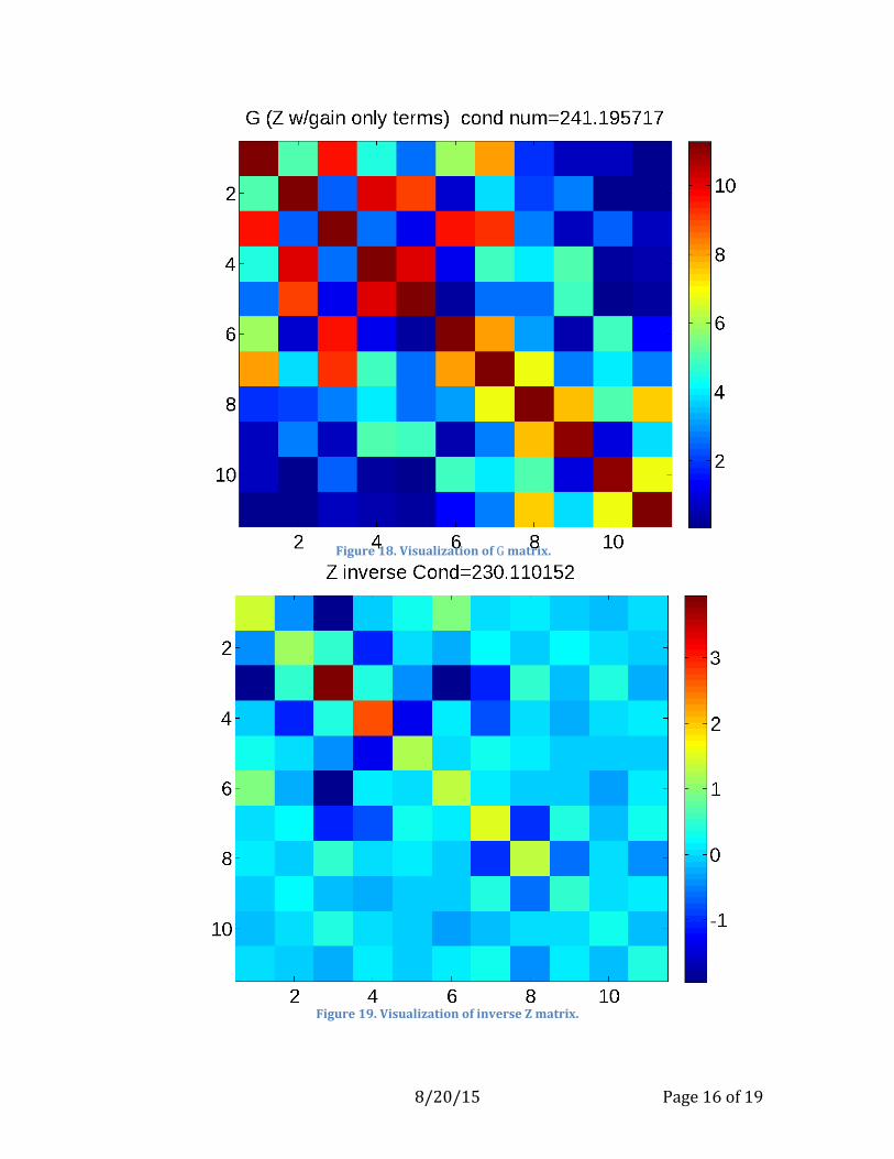
Using the gains in Fig. 17, the BG Z matrix can be computed. The BG G matrix is illustrated in Fig. 18. With the pre-averaged MRFs, the matrix condition is reduced to 241. Figure 19 shows the inverse of the BG Z matrix, where particular values of γ and ω are used. Figure 20 shows a plot of the condition number versus γ. The corresponding estimate of Tb is shown in Fig. 21. Note that the result now resembles the first case with the issues of the matrix inversion are resolved. The new Tb estimate is much closer to the AVE estimate.

8/20/15 Page15of19



8/20/15 Page16of19



8/20/15 Page17of19


Figure21.(blueline)BGTbestimateversusgammavalue.(redline)AVEvalue

8/20/15 Page18of19

3 Conclusion

Based on the analysis presented in this report, it is recommended that multiple measurements at one quantized grid location be averaged prior to applying the BG algorithm. Figure 22 shows the results with the corrected BG algorithm.

4 References

Backus,G.E.,andJ.F.Gilbert,1967.Numericalapplicationsofaformalismforgeophysicalinverseproblems,Geophys.J.R.Astron.Soc.,vol.13,pp.247–276.Backus,G.E.,andJ.F.Gilbert,1968.ResolvingpowerofgrossEarthdata,Geophys.J.R.Astron.Soc.,vol.16,pp.169–205.Caccin,B.,C.Roberti,P.Russo,andA.Smaldone,1992.TheBackus–Gilbertinversionmethodandtheprocessingofsampleddata,IEEETrans.SignalProcessing,vol.40,pp.2823–2825.Chakraborty,P.,A.Misra,T.Misra,andS.S.Rana,2008.BrightnessTemperatureReconstructionUsingBGI,IEEETrans.Geosci.RemoteSensing,vol.46,no.6,pp.1768–1773.Farrar,M.R.,andE.A.Smith,1992.SpatialresolutionenhancementofterrestrialfeaturesusingdeconvolvedSSM/Ibrightnesstemperatures,IEEETrans.Geosci.RemoteSensing,vol.30,pp.349–355.Long,D.G.,andD.L.Daum,1998.SpatialResolutionEnhancementofSSM/IData,”IEEETransactionsonGeoscienceandRemoteSensing,Vol.36,No.2,pp.407‐417. Long,D.G.,P.Hardin,andP.Whiting,1993.ResolutionEnhancementofSpaceborneScatterometerData,IEEETransactionsonGeoscienceandRemoteSensing,Vol.31,No.3,pp.700‐715. Poe,G.A.,1990.Optimuminterpolationofimagingmicrowaveradiometerdata,IEEETrans.Geosci.RemoteSensing,vol.28,pp.800–810. Robinson,W.D.,C.Kummerow,andW.S.Olson,1992.AtechniqueforenhancingandmatchingtheresolutionofmicrowavemeasurementsfromtheSSM/Iinstrument,IEEETrans.Geosci.RemoteSensing,vol.30,pp.419–429.Sethmann,R.,B.A.Burns,andG.C.Heygster,1994.SpatialresolutionimprovementofSSM/Idatawithimagerestorationtechniques,IEEETrans.Geosci.RemoteSensing,vol.32,pp.1144‐1151.

8/20/15 Page19of19

Stephens,P.J.,andA.S.Jones.2002.AcomputationallyefficientdiscreteBackus‐Gilbertfootprint‐matchingalgorithm.IEEETrans.Geosci.RemoteSensing,vol.40,no.8,pp.1865‐1878.Stogryn,A.,1978.Estimatesofbrightnesstemperaturesfromscanningradiometerdata,IEEETrans.AntennasPropagat.,vol.AP‐26,pp.720–726.

Figure22.SameasFig.1butwiththeBGalgorithm recommendationsimplemented.

implementation of bg - nsidc

Documents