Final Degree Project in Telecommunications engineering

Implementation of GNSS ionospheric models in gLAB

Author:

Deimos Ibanez Segura

Department of Applied Mathematics IV

Universitat Politecnica de Catalunya (UPC)

Year: 2014

Director:

Prof. Jose Miguel Juan ZornozaProf. Jaume Sanz Subirana

Tutor:

Adria Rovira Garcia

Resum

L’objectiu d’aquest Projecte Final de Carrera es incorporar els models ionosfericsdisponibles per a GNSS (Global Navigation Satellite System o Sistema Global deNavegacio per Satel.lit) en el programa gLAB (veure capıtol 2). Aquesta actu-alitzacio era necessaria ja que han aparegut nous models ionosferics ja acabatso d’altres que estan en la fase final de proves. Alguns d’ells s’han desenvolupatper a noves constel.lacions de satel.lits (com el model NeQuick per a Galileo-el sistema global de navegacio per satel.lit europeu-), altres s’han creat pera millorar la precisio (com el model F-PPP -Fast Precise Point Positioning oPosicionament de Punts Precıs i Rapid-). En qualsevol cas, actualitzar gLABfara que el programa tingui els models de darrera generacio en processament deGNSS.

Els models ionosferics son utilitzats durant la navegacio per satel.lit, per tantes donara una introduccio tant per a la ionosfera (veure capıtol 3), com per ala navegacio per satel.lit (veure capıtol 1). L’objectiu d’aquestes introduccionses donar una guia basica dels principis dels models ionosferics, accessible fins itot per als lectors que no estiguin familiaritzats amb GNSS.

Resumen

El objetivo de este Proyecto Final de Carrera es incorporar los modelos ionosfericosdisponibles para GNSS (Global Navigation Satellite System o Sistema Global deNavegacion por Satelite) en el programa gLAB (ver capıtulo 2). Esta actu-alizacion era necesaria ya que han aparecido nuevos modelos ionosfericos yaacabados u otros que estan en la fase final de pruebas. Algunos de ellos se handesarrollado para nuevas constelaciones de satelites (como el modelo NeQuickpara Galileo -el sistema global de navegacion por satelite europeo-), otros se hancreado para mejorar la precision (como el modelo F-PPP -Fast Precise PointPositioning o Posicionamento de Puntos Preciso y Rapido). En cualquier caso,actualizar gLAB hara que el programa tenga los modelos de ultima generacionen procesamiento de GNSS.

Los modelos ionosfericos son utilizados durante la navegacion por satelite, portanto se hara una introduccion tanto para la ionosfera (ver capıtulo 3), comopara la navegacion por satelite (ver capıtulo 1). El objetivo de estas intro-ducciones es dar una guıa basica de los principios de los modelos ionosfericos,accesible incluso a lectores no familiarizados con GNSS.

Abstract

The objective of this Final Degree Project is to incorporate the ionosphericmodels available for Global Navigation Satellite System (GNSS) (Global Nav-igation Satellite System) in gLAB software (see chapter 2). This update wasnecessary due to the appearance of new ionospheric models already finishedor others which are in the final testing phase. Some of them have been de-veloped for new satellite constellations (such as NeQuick model for EuropeanGlobal Navigation Satellite System (Galileo) -the european global navigationsatellite system-), others have been created for improving accuracy (like FastPrecise Point Positioning (F-PPP) model -Fast Precise Point Positioning-). Inany case, updating gLAB will make the program to be in the state-of-art inGNSS processing.

Ionospheric models are used during satellite navigation, so a proper introductionwill be made for both the ionosphere (see chapter 3) and the satellite navigation(see chapter 1). The objective of these introductions are to give a basic guidefor the principles of ionospheric models in satellite navigation, accesible even forreaders not familiarized with GNSS.

Contents

Resum III

Resumen V

Abstract VII

List of Figures XIII

List of Tables XVII

Acronyms XIX

1 Introduction 1

2 gLAB description 5

2.1 Main gLAB features . . . . . . . . . . . . . . . . . . . . . . . . 6

2.2 Graphical User Interface (GUI) . . . . . . . . . . . . . . . . . . 7

2.2.1 Positioning tab . . . . . . . . . . . . . . . . . . . . . . 8

2.2.2 Analysis tab . . . . . . . . . . . . . . . . . . . . . . . . 9

2.3 Data Processing Core (DPC) . . . . . . . . . . . . . . . . . . . 10

2.4 gLAB positioning example . . . . . . . . . . . . . . . . . . . . . 11

3 Ionospheric models 17

X CONTENTS

3.1 Two frequency ionosphere models . . . . . . . . . . . . . . . . 20

3.1.1 Ionosphere-free combination . . . . . . . . . . . . . . . 20

3.2 Single frequency ionosphere models . . . . . . . . . . . . . . . . 21

3.2.1 Klobuchar model . . . . . . . . . . . . . . . . . . . . . 21

3.2.2 BeiDou model . . . . . . . . . . . . . . . . . . . . . . . 24

3.2.3 NeQuick model . . . . . . . . . . . . . . . . . . . . . . 25

3.2.4 GIM (IONEX) model . . . . . . . . . . . . . . . . . . . 26

3.2.5 F-PPP model . . . . . . . . . . . . . . . . . . . . . . . 28

4 User interface changes and testing 29

4.1 User interface . . . . . . . . . . . . . . . . . . . . . . . . . . . 30

4.1.1 Input tab . . . . . . . . . . . . . . . . . . . . . . . . . . 30

4.1.2 Modelling tab . . . . . . . . . . . . . . . . . . . . . . . 32

4.1.3 Filter tab . . . . . . . . . . . . . . . . . . . . . . . . . . 33

4.2 Testing . . . . . . . . . . . . . . . . . . . . . . . . . . . . . . . 34

5 gLAB applications 37

5.1 Klobuchar excessive period . . . . . . . . . . . . . . . . . . . . 37

5.2 Ionospheric model comparison . . . . . . . . . . . . . . . . . . 45

5.3 Other studies where gLAB has been used as a Data ProcessingTool . . . . . . . . . . . . . . . . . . . . . . . . . . . . . . . . 49

6 Conclusion 51

A List of days with Klobuchar discontinuity 53

B Multi-platform arrangements 55

B.1 Windows . . . . . . . . . . . . . . . . . . . . . . . . . . . . . . 55

B.2 Macintosh . . . . . . . . . . . . . . . . . . . . . . . . . . . . . 57

CONTENTS XI

C F-PPP v0.50 59

Acknowledgments 63

Bibliography 65

List of Figures

1.1 GPS, GLONASS, Galileo and BeiDou satellites . . . . . . . . . . 2

1.2 GNSS architecture. . . . . . . . . . . . . . . . . . . . . . . . . 2

1.3 GPS, GLONASS, Galileo and BeiDou frequency bands . . . . . 3

2.1 gLAB GUI initial screen . . . . . . . . . . . . . . . . . . . . . . 7

2.2 gLAB GUI initial Positioning tab . . . . . . . . . . . . . . . . . 8

2.3 gLAB GUI initial Analysis tab . . . . . . . . . . . . . . . . . . . 9

2.4 gLAB Input tab example . . . . . . . . . . . . . . . . . . . . . 11

2.5 gLAB Preprocess tab example . . . . . . . . . . . . . . . . . . 12

2.6 gLAB Modelling tab example . . . . . . . . . . . . . . . . . . . 13

2.7 gLAB Filter tab example . . . . . . . . . . . . . . . . . . . . . 13

2.8 gLAB Output tab example . . . . . . . . . . . . . . . . . . . . 14

2.9 gLAB Analysis tab example . . . . . . . . . . . . . . . . . . . . 14

2.10 NEU positioning error . . . . . . . . . . . . . . . . . . . . . . . 15

3.1 TEC content examples . . . . . . . . . . . . . . . . . . . . . . 19

3.2 Klobuchar model layout . . . . . . . . . . . . . . . . . . . . . . 21

3.3 Ionospheric Pierce Point (IPP), vertical and slant delay illustration 22

3.4 Typical Klobuchar values example . . . . . . . . . . . . . . . . 24

3.5 The five regions defined in NeQuick model . . . . . . . . . . . . 25

XIV LIST OF FIGURES

3.6 Global Ionospheric Maps (GIM) four point interpolation algo-rithm definition . . . . . . . . . . . . . . . . . . . . . . . . . . 27

4.1 IONEX in gLAB input tab . . . . . . . . . . . . . . . . . . . . . 30

4.2 F-PPP in gLAB input tab . . . . . . . . . . . . . . . . . . . . . 31

4.3 DCB in gLAB input tab . . . . . . . . . . . . . . . . . . . . . . 31

4.4 Ionospheric corrections in gLAB modelling tab . . . . . . . . . . 32

4.5 Tropospheric corrections in gLAB modelling tab . . . . . . . . . 32

4.6 P1-P2 corrections in gLAB modelling tab . . . . . . . . . . . . 33

4.7 Ionospheric RMSE in gLAB filter tab . . . . . . . . . . . . . . . 33

4.8 Generic test script diagram . . . . . . . . . . . . . . . . . . . . 35

4.9 Examples of difference between gLAB and reference . . . . . . . 36

5.1 Typical Klobuchar ionospheric corrections for all satellites . . . . 38

5.2 Abnormal Klobuchar ionospheric corrections for all satellites . . 38

5.3 Typical Klobuchar ionospheric correction for a single satellite . . 39

5.4 Abnormal Klobuchar ionospheric corrections for a single satellite 39

5.5 Klobuchar gap values during GPS lifetime in northern hemisphere 40

5.6 Klobuchar gap values during GPS lifetime in southern hemisphere 40

5.7 Klobuchar gap values during GPS lifetime in function of geo-magnetic latitude . . . . . . . . . . . . . . . . . . . . . . . . . 41

5.8 Corrected Klobuchar ionospheric corrections for all satellites . . 42

5.9 Corrected Klobuchar ionospheric correction for a single satellite . 42

5.10 Positioning error in north component between nominal and cor-rected Klobuchar model . . . . . . . . . . . . . . . . . . . . . . 43

5.11 Positioning error in east component between nominal and cor-rected Klobuchar model . . . . . . . . . . . . . . . . . . . . . . 44

5.12 Positioning error in up component between nominal and cor-rected Klobuchar model . . . . . . . . . . . . . . . . . . . . . . 44

LIST OF FIGURES XV

5.13 Positioning error with Klobuchar model . . . . . . . . . . . . . 45

5.14 Positioning error with NeQuick model . . . . . . . . . . . . . . 46

5.15 Positioning error with IGS-GIM model . . . . . . . . . . . . . . 46

5.16 Positioning error with F-PPP model . . . . . . . . . . . . . . . 47

5.17 F-PPP vs ionospheric models . . . . . . . . . . . . . . . . . . . 48

List of Tables

5.1 RMS of 3D positioning error for station hofn, DoY 319, Year 2013 47

5.2 Processing time of 3D positioning error for station hofn, DoY319, Year 2013 (full day) . . . . . . . . . . . . . . . . . . . . . 47

A.1 List of days with Klobuchar discontinuity . . . . . . . . . . . . . 54

A.2 Percentage of days with Klobuchar discontinuity . . . . . . . . . 54

Acronyms list

ANTEX ANTenna EXchange format

ARNS Aeronautical Radio Navigation Service

ASCII American Standard Code for Information Interchange

BeiDou Big Dipper constellation in Chinese

CPU Central Processing Unit

DAT Data Analysis Tool

DCB Differential Code Bias

DoY Day of Year

DPC Data Processing Core

EGNOS European Geostationary Navigation Overlay System

ESA European Space Agency

F-PPP Fast Precise Point Positioning

FOC Full Operational Capability

gAGE Research group of Astronomy and Geomatics

Galileo European Global Navigation Satellite System

GIM Global Ionospheric Maps

gLAB GNSS-Lab Tool suite

GLONASS GLObal NAvigation Satellite System

GNSS Global Navigation Satellite System

GPS Global Positioning System

GUI Graphical User Interface

XX Acronyms list

IGS International GNSS Service

IONEX IONosphere map EXchange format

IPP Ionospheric Pierce Point

NASA National Aeronautics and Space Administration

NEU North East Up

PPP Precise Point Positioning

PRN Pseudo-Random Noise

QZSS Quasi-Zenith Satellite System

RINEX Receiver INdependent EXchange format

RMS Root Mean Square

RMSE Root Mean Square Error

RNSS Radionavigation Satellite Service

SINEX Solution (Software/technique) INdependent EXchange format

SoL Safety-of-Life

SP3 Standard Product #3

SPP Standard Point Positioning

STEC Slant Total Electron Content

TEC Total Electron Content

TECU Total Electron Content Unit

UPC Technical University of Catalonia

USA United States of America

UT Universal Time

Chapter 1

Introduction

A GNSS system is a constellation of satellites orbiting Earth, continuously trans-mitting signals which enables a user to determine his position in three dimensions(by solving the navigation equations), referenced from the Earth’s center.

The first GNSS to appear was GPS, initially focused on military use, but in 1983it was opened por public use (with limitations). Since that date, the numberof applications using GNSS for scientific, commercial and daily use has beencontinuosly increasing, which has made that nowadays an important chunk ofthe global economy is dependent on GNSS. This fact has made that severalcountries have decided to develop their own system.

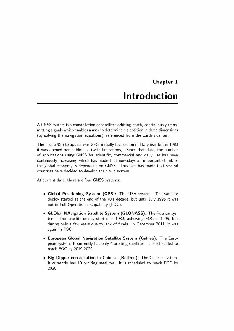
At current date, there are four GNSS systems:

• Global Positioning System (GPS): The USA system. The satellitedeploy started at the end of the 70’s decade, but until July 1995 it wasnot in Full Operational Capability (FOC).

• GLObal NAvigation Satellite System (GLONASS): The Russian sys-tem. The satellite deploy started in 1982, achieving FOC in 1995, butduring only a few years due to lack of funds. In December 2011, it wasagain in FOC.

• European Global Navigation Satellite System (Galileo): The Euro-pean system. It currently has only 4 orbiting satellites. It is scheduled toreach FOC by 2019-2020.

• Big Dipper constellation in Chinese (BeiDou): The Chinese system.It currently has 10 orbiting satellites. It is scheduled to reach FOC by2020.

2 Introduction

Figure 1.1: GNSS satellites: GPS IIR-M (top left), GLONASS-M (topright), Galileo IOV(bottom left) and BeiDou-M (bottom right) from[Sanz et al., 2013].

Each GNSS system is divided in three segments, as shown in figure Fig. 1.2:

• Space Segment: Formed by the orbiting satellites.

• Control Segment: Also known as ground segment, is composed of acontrol center for operating the system, monitoring stations distributedaround the world for data collection and ground antennas for uplink datato the satellites.

• User Segment: Any GNSS receiver capable of determining user coordi-nates from the GNSS signals. For example, any modern smartphone.

Ground Antennas

Control Segment Monitoring Stations

Communication Networks

Master Control Station

User Segment

Satellite Satellite Constellation

Space Segment

Figure 1.2: GNSS architecture from [Sanz et al., 2013].

Introduction 3

Every GNSS system transmits signals in two or more different frequencies. Thereare some frequencies which are exclusive, others are shared with other GNSS sys-tems. The signals transmitted by satellites in these frequencies can be classifiedin three types:

• Carrier: Radio frequency sinusoidal signal at a given frequency.

• Ranging code: Sequences of zeros and ones which allow the receiverto determine the travel time of the radio signal from the satellite to thereceiver. They are called Pseudo-Random Noise (PRN) sequences or PRNcodes.

• Navigation data: A binary-coded message providing information on thesatellite ephemeris (pseudo-Keplerian elements or satellite position andvelocity), clock bias parameters, satellite health status and other comple-mentary information. This data is updated every two hours.

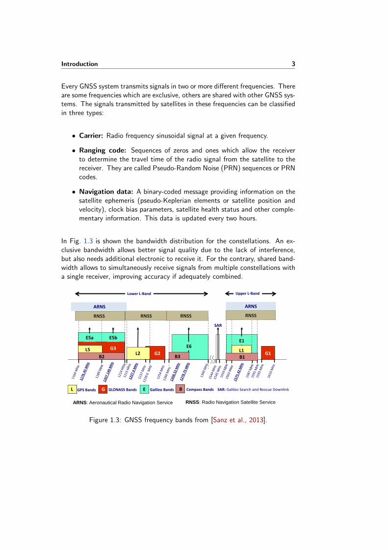
In Fig. 1.3 is shown the bandwidth distribution for the constellations. An ex-clusive bandwidth allows better signal quality due to the lack of interference,but also needs additional electronic to receive it. For the contrary, shared band-width allows to simultaneously receive signals from multiple constellations witha single receiver, improving accuracy if adequately combined.

GLONASS Bands GPS Bands Galileo Bands SAR: Galileo Search and Rescue Downlink

L2 E6

SAR

G1

E1

ARNS

RNSS RNSS RNSS

Lower L-Band Upper L-Band

ARNS

RNSS

ARNS: Aeronautical Radio Navigation Service RNSS: Radio Navigation Satellite Service

E5b E5a

B3 L1 B1

L5 B2

Compass Bands

G3 G2

L G E B

Figure 1.3: GNSS frequency bands from [Sanz et al., 2013].

4 Introduction

As shown in Fig. 1.3, the are two frequencies bands marked as AeronauticalRadio Navigation Service (ARNS), which are exclusive for GNSS signals, thusmaking them suitable for critical operations, such as Safety-of-Life (SoL) oraeronautical uses, hence the name. The rest of the band frequencies are forRadionavigation Satellite Service (RNSS), which are shared with radio locationservices (ground radars).

Furthermore, in Fig. 1.3, it is shown that:

• GPS has three frequencies, L1, L2 and L5. L1 has a civil and a militarysignal, L2 only has a military signal (but in the future will have a civilsignal), and L5 has only a civil signal, but is still is in deployment phase.

• GLONASS has three frequencies, G1, G2, G3. The three of them haveboth a civil and military signal, but the G3 signals is still in deploymentphase)

• Galileo will have 10 civil signals in their frequencies E1, E6 and E5 (E5aand E5b signals are modulated in the same frequency E5). It will haveno military signals, but some of them will have restricted access (only forpublic security authorities use) or for commercial services.

• BeiDou also has three frequencies, B1, B2, B3. B1 and B2 will havepublic signals and restricted signals (commercial or public authorities).B3 only has a restricted signal.

Finally, in order to perform GNSS positioning, the user should use the datagathered from the satellites (ranging code and navigation data) to calculate theposition. As the purpose of this project is the update of gLAB, instead of givinga detailed process of the calculus to retrieve user’s position, a practical examplewith gLAB is done in chapter 2.4.

Chapter 2

gLAB description

The GNSS-Lab Tool suite (gLAB) is an advanced interactive educational mul-tipurpose package to process and analyze GNSS data. The first release of thissoftware package allows full processing capability of GPS data, and partial han-dling of Galileo and GLONASS data.

The gLAB software tool performs a precise modelling of the GNSS observables(code and phase) at the centimeter level, allowing GPS standard and precisepoint positioning (SPP, PPP). gLAB also implements full processing capabili-ties for GPS data and is prepared to allocate future module updates, such as theexpansion to Galileo and GLONASS systems, EGNOS and differential process-ing. It is capable of reading a variety of standard formats such as RINEX-3.00,SP3, ANTEX or SINEX files, among others. Moreover, functionality is alsoincluded for Galileo and GLONASS, being able to perform some data analysiswith real multi-constellation data.

gLAB is flexible, able to run under Linux and Windows operating systems (OS)and it is provided free of charge by European Space Agency (ESA) to Universitiesand GNSS professionals. It is programmed in C and Python languages and isdivided in three main software modules:

• The Data Processing Core (DPC)

• The Data Analysis Tool (DAT)

• The Graphical User Interface (GUI)

The DPC implements all the data processing algorithms and can be executedin command line. The DAT provides a plotting tool for the data analysis. TheGUI consists in different graphic panels for a user friendly managing of both theDPC and DAT. Both the DPC and DAT modules may be used independentlyof the GUI, including them in batch files to automatically process GNSS data.

6 gLAB description

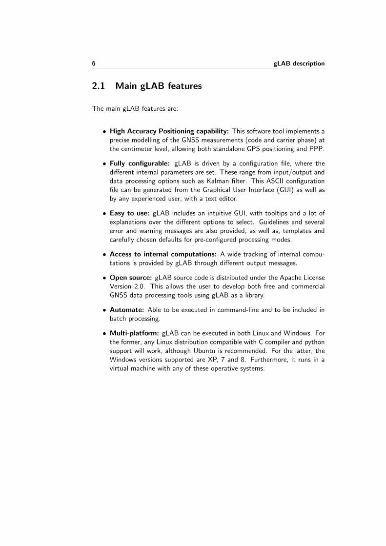
2.1 Main gLAB features

The main gLAB features are:

• High Accuracy Positioning capability: This software tool implements aprecise modelling of the GNSS measurements (code and carrier phase) atthe centimeter level, allowing both standalone GPS positioning and PPP.

• Fully configurable: gLAB is driven by a configuration file, where thedifferent internal parameters are set. These range from input/output anddata processing options such as Kalman filter. This ASCII configurationfile can be generated from the Graphical User Interface (GUI) as well asby any experienced user, with a text editor.

• Easy to use: gLAB includes an intuitive GUI, with tooltips and a lot ofexplanations over the different options to select. Guidelines and severalerror and warning messages are also provided, as well as, templates andcarefully chosen defaults for pre-configured processing modes.

• Access to internal computations: A wide tracking of internal compu-tations is provided by gLAB through different output messages.

• Open source: gLAB source code is distributed under the Apache LicenseVersion 2.0. This allows the user to develop both free and commercialGNSS data processing tools using gLAB as a library.

• Automate: Able to be executed in command-line and to be included inbatch processing.

• Multi-platform: gLAB can be executed in both Linux and Windows. Forthe former, any Linux distribution compatible with C compiler and pythonsupport will work, although Ubuntu is recommended. For the latter, theWindows versions supported are XP, 7 and 8. Furthermore, it runs in avirtual machine with any of these operative systems.

2.2. Graphical User Interface (GUI) 7

2.2 Graphical User Interface (GUI)

The GUI is an interface between the other two components (DPC and DAT).It allows the user to change parameters, and execute the other two programswith proper arguments. The initial screen can be seen in Fig. 2.1, where twomain tabs may be found:

• Positioning: Interfaces with the DPC tool, and allows selecting the dif-ferent processing options.

• Analysis: Interfaces with the DAT tool, and allows selecting the plottingoptions.

Figure 2.1: gLAB GUI initial screen.

A very important feature of gLAB are the tooltips. When the user hovers themouse over a given option, a small box with information about the item isautomatically displayed. These tooltips help the user to understand what is theeffect of each option.

8 gLAB description

2.2.1 Positioning tab

The positioning tab is split into 5 different sections, which correspond to 5different modules inside the DPC:

• INPUT: It is like a “driver” between the input data and the rest of theprogram. This module implements all the input reading capabilities andstores data into the appropriate internal structures.

• PREPROCESS: This module prepares the data for the next module(MODEL). It checks for cycle-slips, pseudorange-carrier phase inconsis-tencies and decimates the data (if required).

• MODEL: This module has all the functions to fully model the receivermeasurements. It implements several kinds of models, which can be en-abled or disabled at will.

• FILTER: This module implements a configurable Kalman filter, and ob-tains the estimations of the required parameters.

• OUTPUT: This module outputs the data obtained from the FILTER.

The GUI also provides two “data processing templates”, shown as buttons inthe lower center part of the interface with labels “SPP Template” and “PPPTemplate” (see Fig. 2.2). Those “templates” automatically configure the ap-propriate options to carry out the desired data processing strategy.

Figure 2.2: gLAB GUI initial Positioning tab.

2.2. Graphical User Interface (GUI) 9

2.2.2 Analysis tab

The analysis tab allows configuring all the visualization options for the DAT,as shown in Fig. 2.3. There are two different areas. On the upper part, theuser finds all the templates buttons. In this case, the templates are a set ofpreconfigured plotting options for the Graphic Details section. Clicking on anybutton will load all the corresponding options, allowing modifying or plottingthem directly.

On the lower part, the user can configure a plot from scratch using the “GlobalGraphic Parameters” section below the templates. The GUI can accommodateup to four plots, (i.e. four different data series in the same graphic) althoughthe DAT program has no plot number limitation when executed independentlyfrom the command line.

Finally, it is only to be remarked that while there are some common data thatneeds to be uploaded only once per graphic, user can fine tune different optionsof the individual plots, providing full flexibility.

Figure 2.3: gLAB GUI initial Analysis tab.

10 gLAB description

2.3 Data Processing Core (DPC)

The DPC is the processing tool of gLAB, and it has been programmed in C. Itis:

• Easy to use for an advanced user.

• Modularized, in order to incorporate future updates.

• Optimized for CPU and memory usage.

The options of the DPC and GUI are basically the same with some exceptionsthat provide further flexibility. The DPC can be executed with the “-help”argument, which provides detailed information of the possible arguments. It isalso worth mentioning that the DPC can also read the processing options from aconfiguration file, allowing an easy repeatability of results and automatic batchprocessing.

The DPC can work in four different modes:

• Positioning Mode: “Standard” mode, where all the processing is doneand the position solution for a receiver is provided as OUTPUT messages.The minimum parameters required for this mode are an input observationfile and orbit and clock products (broadcast or precise). Using preciseproducts will also require the use of an ANTEX file.

• Show Input Mode: This mode only reads an input RINEX observationfile and prints its measurements. No orbit nor clock products should beprovided (if provided, gLAB will switch to Positioning Mode).

• Product Comparison Mode: This mode reads and compares two differ-ent sources of orbit and clock products. In order to use this mode, twodifferent orbit and clock products should be provided. This mode outputsthe SATDIFF, SATSTAT and SATSTATTOT messages.

• Show Product Mode: This mode reads a single source of orbit and clockproducts. In order to use this mode, a single orbit and clock productshould be provided. This mode outputs SATPVT messages with thesatellite coordinates and clocks.

2.4. gLAB positioning example 11

2.4 gLAB positioning example

In this section a simple standard positioning will be done with gLAB. Althoughit is the least accurate, it is commonly used in mobile devices due to they onlywork in single frequency.

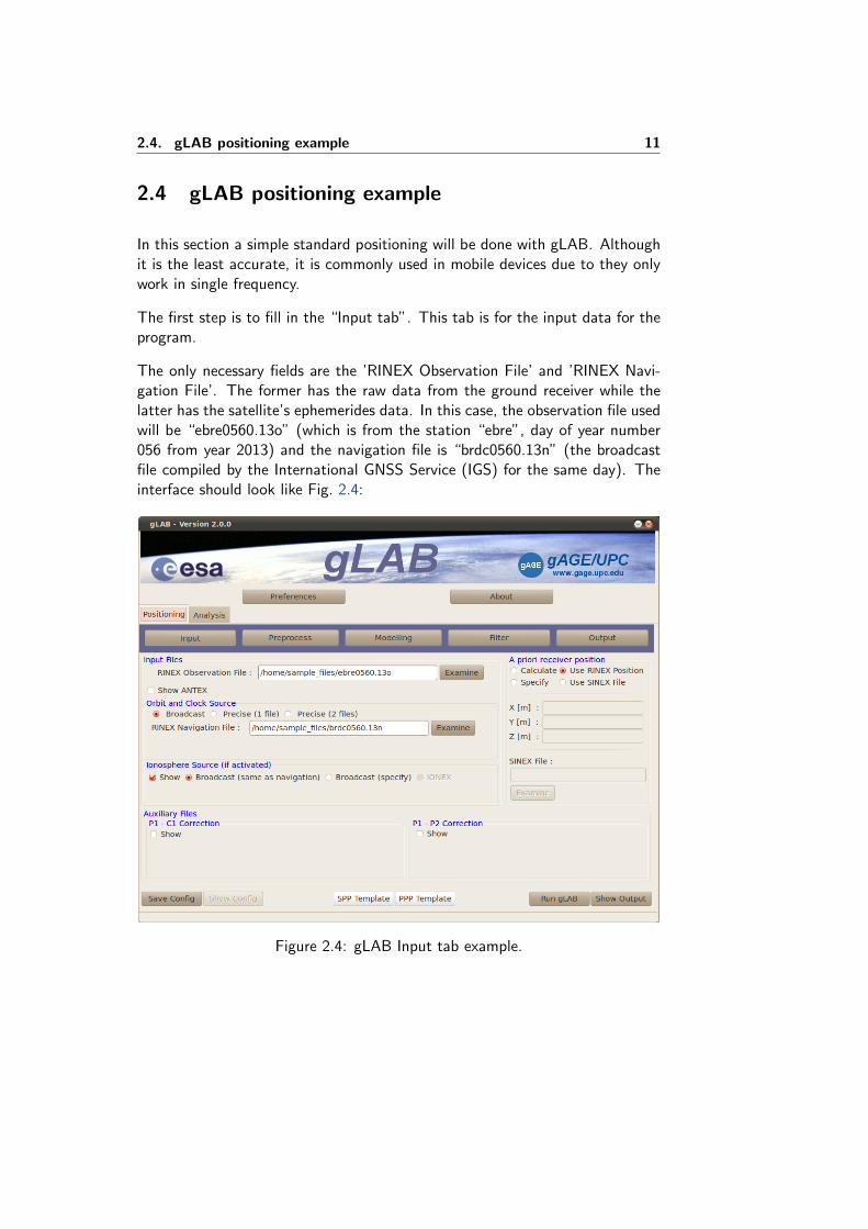
The first step is to fill in the “Input tab”. This tab is for the input data for theprogram.

The only necessary fields are the ’RINEX Observation File’ and ’RINEX Navi-gation File’. The former has the raw data from the ground receiver while thelatter has the satellite’s ephemerides data. In this case, the observation file usedwill be “ebre0560.13o” (which is from the station “ebre”, day of year number056 from year 2013) and the navigation file is “brdc0560.13n” (the broadcastfile compiled by the International GNSS Service (IGS) for the same day). Theinterface should look like Fig. 2.4:

Figure 2.4: gLAB Input tab example.

12 gLAB description

The next step is to check the “Preprocess tab”. The purpose of this tab is tocheck for data consistency and validity. Some of the checks are:

• Satellite health: Check if the health bits in the RINEX navigation mes-sage are “0”. If not “0”, it means that a satellite is not sending validdata.

• Cycle slip: When using the phase of the satellite signal (not used inthis example), the measurements must be continuous. When a cycle slipoccurs, measurements are not continuous and they have to be reset.

It is enough to use the default configuration. More information on each optionscan be gathered by hovering over them until its tooltip appears. The interfaceshould look like Fig. 2.5:

Figure 2.5: gLAB Preprocess tab example.

2.4. gLAB positioning example 13

In the “Modelling tab”, we can select the different models to compensate theerrors produced for electronic and environmental effects in the signal, such asthe electronic delays or atmospheric effects.

The default options should be used. The interface should look like Fig. 2.6:

Figure 2.6: gLAB Modelling tab example.

In the “Filter tab”, represents the last step in the calculus. After checking forsignal consistency and modelling error sources, a mathematic algorithm, namedfilter, uses all the data to calculate the current position, using also data fromthe previous iteration.

The default options should be used, though manipulating the filter optionsrequires advanced knowledge. The interface should look like Fig. 2.7:

Figure 2.7: gLAB Filter tab example.

14 gLAB description

Finally, in the “Output tab”, we can select which messages are printed in theoutput file. gLAB can print many values from its internal calculations.

The default options are recommended. At least the OUTPUT messages shouldbe activated. The interface should look like Fig. 2.8:

Figure 2.8: gLAB Output tab example.

Once the configuration is finished, click on the “Run gLAB” button on thebottom right hand side of the screen to start the computations. Once finished,we will switch to the ‘Analysis tab’.

In the “Analysis tab”, each of the buttons are for predefined plots. Clicking onthe “NEU positioning error” button will automatically set the configuration forprinting the measurement error in the three axis (North East Up (NEU)). Theinterface should look like Fig. 2.9:

Figure 2.9: gLAB Analysis tab example.

2.4. gLAB positioning example 15

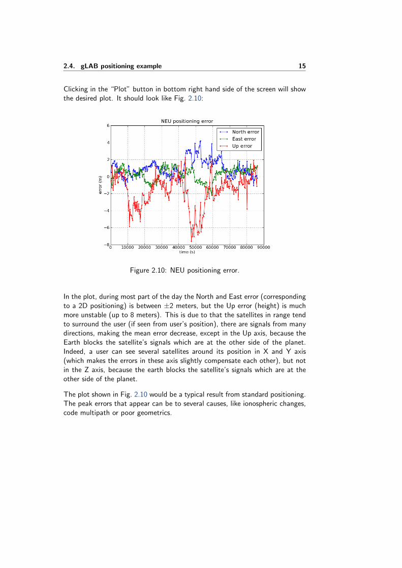
Clicking in the “Plot” button in bottom right hand side of the screen will showthe desired plot. It should look like Fig. 2.10:

Figure 2.10: NEU positioning error.

In the plot, during most part of the day the North and East error (correspondingto a 2D positioning) is between ±2 meters, but the Up error (height) is muchmore unstable (up to 8 meters). This is due to that the satellites in range tendto surround the user (if seen from user’s position), there are signals from manydirections, making the mean error decrease, except in the Up axis, because theEarth blocks the satellite’s signals which are at the other side of the planet.Indeed, a user can see several satellites around its position in X and Y axis(which makes the errors in these axis slightly compensate each other), but notin the Z axis, because the earth blocks the satellite’s signals which are at theother side of the planet.

The plot shown in Fig. 2.10 would be a typical result from standard positioning.The peak errors that appear can be to several causes, like ionospheric changes,code multipath or poor geometrics.

Chapter 3

Ionospheric models

The Earth’s atmosphere is a gaseous cover surrounding the planet and is retainedby the Earth gravitational field. The different regions of the atmosphere canbe characterized by temperature, composition and ionization. The atmospherechanges the speed and direction of propagation of radio signals, phenomenonwhich is referred to as refraction. These changes affect the signal transit time,which is the basic measurement in GNSS. The variation in signal directionis generally insignificant in both layers, but the speed variations can lead upto 60 meters difference in pseudorange measurements and can not be directlymeasured. Therefore, it is required a mathematic model to compensate thiseffect. For satellite signals, which goes through atmosphere, there are tworelevant layers, the troposhere and the ionosphere.

The troposphere, is a region of electrically neutral gaseous. It is found betweenEarth’s surface and an altitude of about 60 km, and it is a non dispersivemedium, meaning that the changes are independent from the frequency. Aconsequence of not being a dispersive medium is that the tropospheric refractioncannot be removed with dual-frequency measurements, hence being compulsorythe use of a mathematic model (this is the main reason why ESA’s troposphericmodel has been also included in this update, see section 4.1.2).

The troposhere refraction on GNSS signals appears as an extra delay in themeasurement of the signal travel time. This delay is separable in two compo-nents, the hydrostatic component delay (90% of the total delay) and the wetcomponent delay (10%). The former is caused by dry gases in the troposphere,and has a slow and predictible variation (it is the variation predicted by thetroposheric models). The latter is caused by the water vapour and condensedwater in form of clouds, and therefore depends on weather conditions. Thiscomponent delay is small (about tens of centimeters) and is estimated in thenavigation filter only in precise navigation. No more details will be given abouttroposphere, though it is not the subject of study in this project.

18 Ionospheric models

Focusing now on the ionosphere, it is the atmosphere region extends from aheight from 50 to 2000 km above the Earth. This region contains a partiallyionised medium, as a result of solar X and Extreme UltraViolet (EUV) raysin the solar radiation and the incidence of charged particles, which ionize thedifferent neutral atmospheric components.

The propagation speed of GNSS electromagnetic signals in the ionosphere de-pends on its electron density, which is typically driven by two main processes.During the day, the Sun’s radiation ionises neutral atoms to produce free elec-trons and ions. During the night, the recombination process prevails, where freeelectrons are recombined with ions to produce neutral particles, which leads toa reduction in the electron density. The electron density (Ne) in the ionospherechanges with height, having a maximum of Ne ' 1011 to 1012 e−/m3 around300− 500 km.

The ionosphere is a dispersive medium, which means that it is frequency depen-dent. Furthermore, dispersive mediums reflect signals lower than a thresholdfrequency. For the ionosphere the threshold is at 106 Hz, which is lower thanGNSS signals, that are at the order of 1 GHz (= 109 Hz), thus allowing satellitesignals to go through.

To compute the difference between the measured range (with frequency f signal)and the Euclidean distance between the satellite and receiver, the relation is thefollowing (from [Sanz et al., 2013]):

∆ionoph,f = −40.3

f2

∫Ne dl, ∆iono

gr,f = +40.3

f2

∫Ne dl (3.1)

The differences ∆ionoph,f and ∆iono

gr,f are called the phase and code ionosphericrefraction, respectively, and the integral is defined as the Slant TEC, or SlantTotal Electron Content (STEC)

STEC =

∫Ne dl (3.2)

As it can be seen in (3.1), phase measurements are advanced on crossing theionosphere, that is a negative delay, while the code measurements undergo apositive delay.

Ionospheric models 19

Usually, the STEC is given in TEC units (TECUs), where 1 TECU = 1016 e−/m2

and the ionospheric delay If (at the frequency f) is written as

If ≡ ∆ionogr,f = αf STEC (units: metres of delay) (3.3)

with

αf =40.3 · 1016

f2msignal delay(at frequencyf)

/TECU (where f is in Hz) (3.4)

The TEC, and hence the ionospheric refraction, depend on the geographic lo-cation of the receiver, the hour of day and the intensity of the solar activity.Figure 3.1a (left) shows a vertical TEC map of the geographic distribution ofthe TEC, where the equatorial anomalies are clearly depicted around the geo-magnetic equator. The figure on the right 3.1b shows the 11-year solar cyclewith a solar flux plot.

(a) TEC Map (b) Solar flux

Figure 3.1: The map on the left shows the vertical Total Electron Content inTECUs at 19UT on 26 June 2000 (1 TECU ' 16 cm of delay in the GPS L1signal). The plot on the right shows the evolution of the solar flux during thelast solar cycles (from [Sanz et al., 2013]).

20 Ionospheric models

3.1 Two frequency ionosphere models

3.1.1 Ionosphere-free combination

As explained above, ionosphere effects are frequency dependent. In concrete,first order effects depend on 99.9% on the inverse of squared signal frequency.Therefore, ionosphere effect can be eliminated through a linear combinationshown in (3.5), in example the ionosphere free combination:

Riono−free =f21R1 − f2

2R2

f21 − f2

2(3.5)

Where R1 and R2 are the pseudorange or carrier values measured in both fre-quencies, f1 and f2 are the signal frequencies, and Riono−free is the resultingvalue without ionosphere effects.

Although it is not a mathematic model, it is by far the most effective and sim-plest. Nevertheless, it has two important drawbacks: it requires dual frequencyreceivers (many of them are single receivers to reduce costs and space) and,obviously, it requires two frequencies.

For GPS system, there is only one civilian signal in one frequency. Neverthe-less, many commercial receivers are capable of tracking military signals in bothfrequencies, but at the cost of losing some accuracy. In the near future, it isplanned to create a new civil signal in the second GPS frequency. Regarding theother GNSS system, GLONASS has two public civil signals since 2004, whileGalileo and BeiDou will have them at the moment they reach Full OperationalCapability (FOC).

It must be pointed out that the Precise Point Positioning (PPP) uses code andcarrier phase measurements in the ionosphere-free combination to remove theionospheric refraction, because it is one of the effects that is more difficult tomodel accurately.

3.2. Single frequency ionosphere models 21

3.2 Single frequency ionosphere models

Single frequency receivers need to apply a model to remove ionospheric effects.As mentioned above, ionosphere effects are greatly variable, hence it is necessaryto adjust model parameters periodically. GPS, Galileo and BeiDou broadcastthis parameters through the navigation file transmitted by the satellites, andare updated daily. GLONASS does not broadcast any ionospheric model, butany of the existing models can be applied to this constellation by applying acorrection factor given by their relative squared frequency ratio.

3.2.1 Klobuchar model

Klobuchar model was designed to minimize user computational complexity anduser computer storage so as to keep a minimum number of coefficients to betransmitted. It is based on an empirical approach ([Klobuchar, 1987]) and itis estimated to reduce the error by 50% (in RMS). In the navigation message,these coeficients are given in the lines labeled as “IONALPHA” and “IONBETA”in RINEX version 2 or “GPSA” and “GPSB” in version 3 in the header tobroadcast its parameters.

This model is independent from user’s position (it does not apply any specificcorrection for any region) and the ionosphere is modeled as single layer at analtitude of 350 km. This model assumes there is a constant delay of 5 ns duringnight time and a half-cosine function in daytime that is centered at the 14thhour (2 pm) of local time (as shown in Fig. 3.2), whose amplitude and periodare given as a function of the eight parameters broadcasted in the navigationmessage.

Figure 3.2: Klobuchar model layout from [Sanz et al., 2013]

22 Ionospheric models

To compute the slant delay, it is necessary to first calculate the IonosphericPierce Point (IPP), which is the intersection of the ray with the ionosphericlayer at 350 km in height, then compute the vertical delay at the IPP, andfinally get the slant delay by multiplying by and obliquity factor (also called themapping function, see Fig 3.3 and equation 3.14).

Figure 3.3: Ionospheric Pierce Point (IPP), vertical and slant delay illustration[Sanz et al., 2013]

The Klobuchar algorithm to run in a single-frequency receiver is provided asfollows [Klobuchar, 1987].

Given the user’s approximate geodetic latitude ϕu and longitude λu, the el-evation angle E and azimuth A of the observed satellite and the Klobucharcoefficients αn and βn broadcasted in the GPS satellite navigation message:

1. Calculate the Earth-centred angle

ψ = π/2− E − arcsin

(RE

RE + hcosE

)(3.6)

2. Compute the latitude of the IPP

φI = arcsin (sinϕu cosψ + cosϕu sinψ cosA) (3.7)

3. Compute the longitude of the IPP

λI = λu +ψ sinA

cosφI(3.8)

4. Find the geomagnetic latitude of the IPP

φm = arcsin (sinφI sinφP + cosφI cosφP cos(λI − λP )) (3.9)

with φP = 78.3◦, λP = 291.0◦ the coordinates of the geomagnetic pole.

3.2. Single frequency ionosphere models 23

5. Find the local time at the IPP

t = 43 200λI/π + tGPS (λI in radians, t in seconds) (3.10)

where 0 ≤ t < 86 400. Therefore:If t ≥ 86 400, subtract 86 400. If t < 0, add 86 400.

6. Compute the amplitude of ionospheric delay

AI =

3∑n=0

αn (φm/π)n (seconds) (3.11)

If AI < 0, then AI = 0.

7. Compute the period of ionospheric delay

PI =

3∑n=0

βn (φm/π)n (seconds) (3.12)

If PI < 72 000, then PI = 72 000.

8. Compute the phase of ionospheric delay

XI =2π(t− 50 400)

PI(radians) (3.13)

9. Compute the slant factor (ionospheric mapping function)

F =

[1−

(RE

RE + hcosE

)2]−1/2

(3.14)

10. Compute the ionospheric time delay

I1=

[5 · 10−9 +AI cosXI

]× F, |XI | < π/2

5 · 10−9 × F, |XI | ≥ π/2(3.15)

The delay I1 is given in seconds and is referred to the GPS L1.

Although this algorithm is provided to estimate the ionospheric delay in theGPS, it can also be used to estimate the ionospheric time delay in other fre-quency signals or for the GLONASS and Galileo signals, as well. Indeed, takinginto account that the ionospheric delay is inversely proportional to the squareof the signal frequency, the delay for any GNSS signal transmitted on frequencyfk is given by

Ik =

(f1fk

)2

I1 (3.16)

24 Ionospheric models

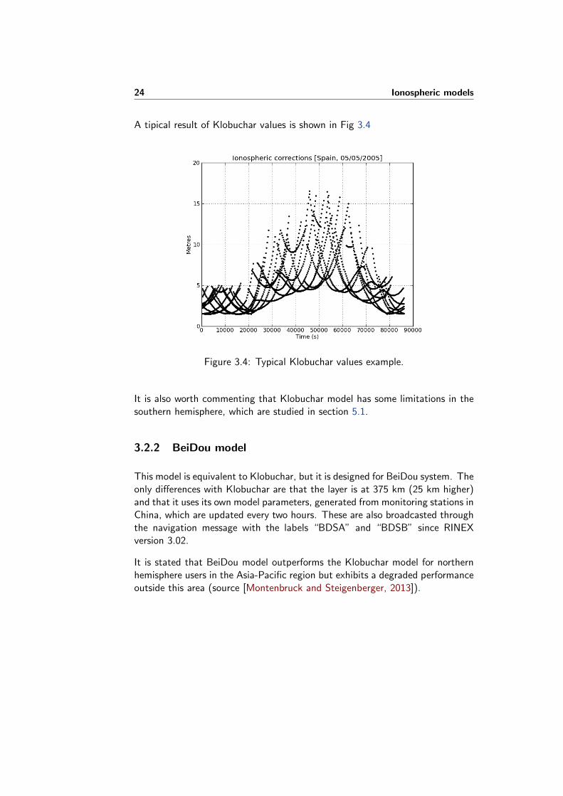
A tipical result of Klobuchar values is shown in Fig 3.4

Figure 3.4: Typical Klobuchar values example.

It is also worth commenting that Klobuchar model has some limitations in thesouthern hemisphere, which are studied in section 5.1.

3.2.2 BeiDou model

This model is equivalent to Klobuchar, but it is designed for BeiDou system. Theonly differences with Klobuchar are that the layer is at 375 km (25 km higher)and that it uses its own model parameters, generated from monitoring stations inChina, which are updated every two hours. These are also broadcasted throughthe navigation message with the labels “BDSA” and “BDSB” since RINEXversion 3.02.

It is stated that BeiDou model outperforms the Klobuchar model for northernhemisphere users in the Asia-Pacific region but exhibits a degraded performanceoutside this area (source [Montenbruck and Steigenberger, 2013]).

3.2. Single frequency ionosphere models 25

3.2.3 NeQuick model

NeQuick model has been designed for Galileo system, and it is based on theoriginal profiler developed by [Di Giovanni and Radicella, 1990]. It is a threedimensional and time dependent ionospheric electron density model, which pro-vides the electron density in the ionosphere as a function of position and time. Ithas five predefined regions (as shown in Fig. 3.5) and has four input parametersthat will be broadcasted in header of the navigation message, in the line labeledas “GAL”. It also uses 13 data files with numerical values that the receiver musthave in order to be able to use the model. These data files are expected to beupdated every 5 years approximately, due to its natural variation.

Northern Region

Northern Middle Region

Equatorial Region

Southern Middle Region

Southern Region

Figure 3.5: The five regions defined in NeQuick model (source[Arbesser-Rastburg, B., 2006])

The algorithm for the Galileo single-frequency receiver is based on the followingsteps1 (from [Arbesser-Rastburg, B., 2006]):

1. Model input values are computed using the navigation message parame-ters.

2. Electron density is calculated for a point along the satellite to receiverpath.

1The algorithm is too long to be explained here, as it is as big as 1/3 of gLAB

26 Ionospheric models

3. Steps 1 and 2 are repeated for many discrete points along the satellitereceiver path. The number and spacing of the points will depend onthe height and they will be a trade-off between integration error andcomputational time and power.

4. All electron density values along the ray are integrated in order to obtainSlant TEC (or STEC).

5. STEC, in TECUs, is converted to metres of slant delay for correctingpseudo-ranges, by

If =40.3 · 1016

f2TEC (where f is in Hz) (3.17)

Note that, as with the Klobuchar model, the ionospheric corrections computedby the NeQuick model can be used for any GNSS signal (GPS, GLONASS,Galileo, etc.) simply by setting the corresponding frequency in (3.17).

3.2.4 GIM (IONEX) model

Global Ionospheric Maps (GIM) is a world-wide map with ionosphere valuesmade by International GNSS Service (IGS). These values are estimated throughdirect measurements, and are provided as a regular grid. Each grid may havedifferent length between points, and may have or more layers. Each grid is givenat a certain epoch in Universal Time (UT), and it may not be at a fixed timeperiod, even though, they are very often published at a rate of 2 hours, with agrid of 2.5 degrees in latitude and 5 degrees in longitude, with a single layer at450 km, but these values are configurable.

The standard file format used for broadcasting ionospheric maps is known asIONosphere map EXchange format (IONEX)[Stefan Schaer, 1998] (this is whyGIM is often called IONEX). In the header of this file it is given the size of thegrid as well as the periodicity. This files are published on a public server thefollowing day, being not provided in real time. Nevertheless, there are predictedGIMs (from two days ahead) in order to allow real time navigation, althoughthe accuracy is worse. These files can be found, for instance, at the public ftpNASA server ftp://cddis.gsfc.nasa.gov/gps/products/ionex/.

3.2. Single frequency ionosphere models 27

The algorithm to compute the ionospheric correction is the following:

1. Find the grid maps which are before and ahead of our current time

2. Select the grid map time before our current time

3. Select the first layer in the current grid map

4. Compute the Ionospheric Pierce Point (IPP) in the current grid map andlayer

5. Find the four points of the grid which are surrounding the IPP

6. Calculate the Weights (Wi) for each grid point, which is the product ofthe unitary distance from the IPP to a grid point in each axis (see Fig. 3.6)

Figure 3.6: Four point interpolation algorithm definition

7. Compute the vertical ionospheric delay, which is the sum of the value ofeach grid point multiplied by its weight (see equation 3.18)

τvpp(φpp, λpp) =4∑

n=1

Wi · τvi (3.18)

8. Compute the mapping function2 for the current IPP

F =RE + h√

(RE + h)2 − (RE · cosE)2(3.19)

Being RE the Earth radius (provided in the IONEX header), h the layeraltitude and E the elevation angle.

2The equation provided corresponds to the “COSZ” function, which is the default if noneis specified in the IONEX header. There are others, like the “QFAC” function, but are rarelyused. gLAB supports “COSZ” and “QFAC” functions.

28 Ionospheric models

9. Calcute the slant delay at the current layer by multiplying the verticaldelay with the mapping function

10. Repeat steps 4 to 9 with all the available layers, adding up the slant delayof the previous layer to the current one

11. Calculate the weight of the current grid map time, which is the unitarydistance between the current time and the grid map time (like in step 6but in only 1 dimension)

12. Multiply the slant delay of the current grid map time by its weight

13. Repeat steps 3 to 12 with the grid map ahead of our current time

14. Sum the slant delay from both grid map time. The result is in TECUs

15. STEC, in TECUs, is converted to metres of slant delay for correctingpseudo-ranges, by

If =40.3 · 1016

f2TEC (where f is in Hz) (3.20)

Like the previous ionospheric models, it can be used with any GNSS signal bysimply setting the corresponding frequency in (3.20).

3.2.5 F-PPP model

The Fast Precise Point Positioning (F-PPP) ionosphere is a real-time world-wideionospheric model for precise navigation developed by the gAGE/UPC researchgroup. It is still in development, but current tests are giving results about oneorder of magnitude better than Klobuchar or NeQuick and several times betterthan the well-known post-processed IGS-GIMs [Rovira-Garcia et al., 2014].

The F-PPP is generated every 5 minutes, and it will be broadcasted throughpublic servers as IONEX files, allowing anyone using the GIM model will be ableto use F-PPP. At the current date, it is using a non-standard file format, whichgLAB is able to read (see appendix C for details).

Chapter 4

User interface changes andtesting

During the update of gLAB, it was intended that all new features available hadto be integrated as additional functions, so the main program structure wasunchanged. This guarantees full compatibility with older versions, as well asavoiding the user the need to re-familiarize with a new Graphical User Interface(GUI).

Furthermore, not only additional ionosphere models have been implemented,but other secondary improvements have been made. These are the capabilityof reading version 3.02 RINEX files and the inclusion of ESA’s tropospheremodel. The former is due to that RINEX version 2 files supports GPS, GalileoGLONASS and geostationary constellations, while version 3.02 can handle allof them (including new japanese QZSS and chinese BeiDou), so it is highlyrecommended to use this version (compulsory for multiple constellations files).The latter was done to complete Galileo models, even though gLAB is stillunable to process Galileo data, it prepares it for a possible future update on thismatter.

30 User interface changes and testing

4.1 User interface

Here are shown the Graphical User Interface (GUI) tabs which have been changedfor the new gLAB version:

4.1.1 Input tab

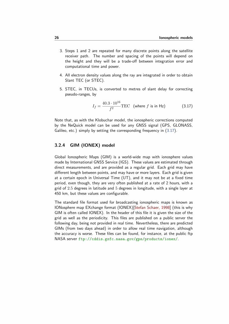
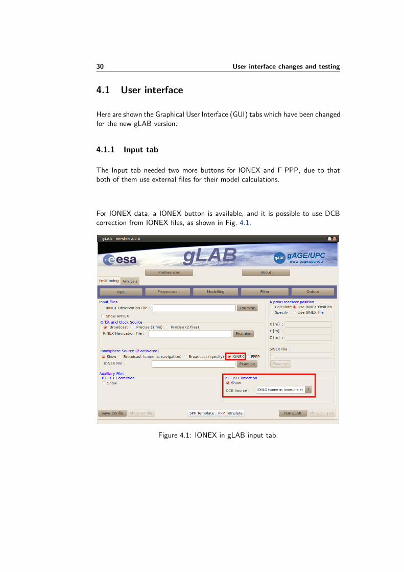
The Input tab needed two more buttons for IONEX and F-PPP, due to thatboth of them use external files for their model calculations.

For IONEX data, a IONEX button is available, and it is possible to use DCBcorrection from IONEX files, as shown in Fig. 4.1.

Figure 4.1: IONEX in gLAB input tab.

4.1. User interface 31

The same changes have been made for F-PPP data, as shown in Fig. 4.2.

Figure 4.2: F-PPP in gLAB input tab.

It is worth highlighting that in both cases, the DCB’s are selected by defaultfrom the same ionospheric source when the IONEX or F-PPP button are press,but it is possible to select DCB data from another IONEX or F-PPP file, asshown in Fig. 4.3.

Figure 4.3: DCB sources in gLAB input tab.

32 User interface changes and testing

4.1.2 Modelling tab

The Modelling tab has not had any significant changes but adding more optionsin the following corrections options:

The first add-on is in the ionospheric correction options, in which NeQuick,Klobuchar(BeiDou), IONEX and F-PPP models have been added, as shown inFig. 4.4 (see section 3.2 for ionospheric model explanation).

Figure 4.4: Ionospheric corrections in gLAB modelling tab.

The second add-on is the ESA’s tropospheric model (in the tropospheric correc-tion list), as shown in Fig. 4.5. It is worth pointing out that if ESA’s troposphericmodel is chosen, Niell mapping is selected by default, because this is the onlymapping accepted by this model.

Figure 4.5: Tropospheric corrections in gLAB modelling tab.

4.1. User interface 33

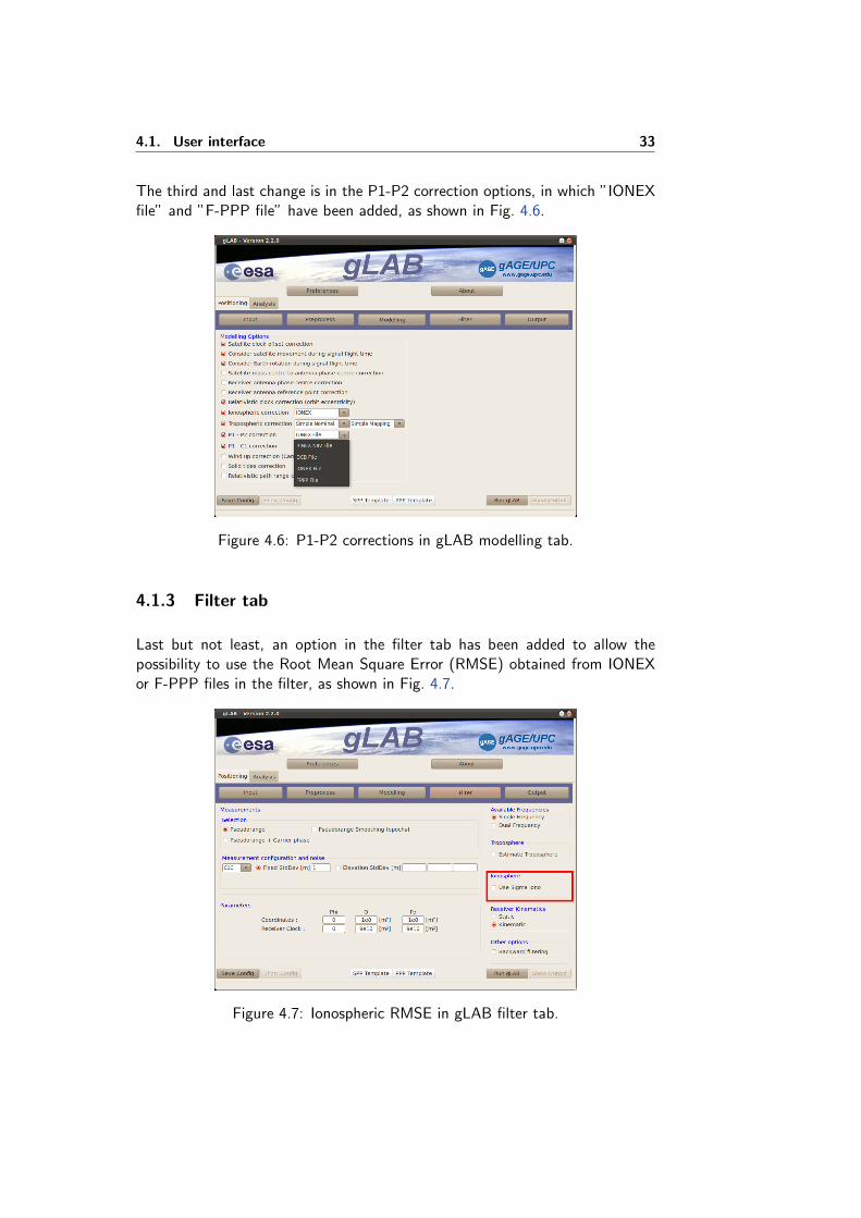
The third and last change is in the P1-P2 correction options, in which ”IONEXfile” and ”F-PPP file” have been added, as shown in Fig. 4.6.

Figure 4.6: P1-P2 corrections in gLAB modelling tab.

4.1.3 Filter tab

Last but not least, an option in the filter tab has been added to allow thepossibility to use the Root Mean Square Error (RMSE) obtained from IONEXor F-PPP files in the filter, as shown in Fig. 4.7.

Figure 4.7: Ionospheric RMSE in gLAB filter tab.

34 User interface changes and testing

4.2 Testing

Once ionospheric models are implemented in gLAB, they need to be checkedto assure their correct functionality. For this purpose, and for each model, anexternal script bash script was created. All of them have the same code exceptfor the ionospheric model used.

The aim of the script is to the test the models in all latitudes and longitudes,so for this purpose, from the station list given, it will sort them in order tomake a grid of stations by latitude and longitude (by default, width will be 5◦

in latitude and 10◦ in longitude). Once done, the script will process one stationin each square (close stations do not provide additional relevant data for thispurpose). If the selected station has no observation data, it will try to processother stations until any of them has data or there are not any stations left inthat range. The system flow chart is shown in Fig. 4.8.

The execution results are given in three files and four figures for each station:

• Files:

� The gLAB output file.

� The output file for the reference model (the format may vary in eachcase).

� A data file containing the time (DoY), the ionospheric values foreach model and the difference between them.

• Figures:

� A figure for gLAB ionospheric model values.

� A figure for the reference ionospheric model values.

� A figure with both model values superimposed.

� A figure with the difference (error) between models.

The most important files are both the difference error data file and figure. Thelatter allows and easy evaluation of the error value, while the former has theabsolute values, where is visible is following common patterns (like day/nightcycles). The exception is for BeiDou model, where there is no third partyprogram for comparing data, nor even broadcast data. For this reason, BeiDoucalculations will be done using Klobuchar’s broadcast data of GPS satellites. Asboth models are very similar, BeiDou results must be very similar too.

4.2. Testing 35

Input: Year, DoY, station list

Sort station list by latitude and

longitude, grouping by ranges of “n”

degrees

Download Navigation and Ionospheric (if

applicable) files

Set initial range as the lowest latitude range with stations

in the list

Select first station in list in

current range

Download station’s observation file

DownloadOK?

Is it the laststation

in range?

Select nextstation

Process with selected

ionospheric model

Calculate difference error betwen gLAB

and reference model

Generate graphs for gLAB, reference model and error

values

Erase observation file

Is it the last range?

Erase navigation and Ionospheric (if

applicable) files

End

Select next range

No

Yes

Yes

No

Yes

No

Figure 4.8: Generic test script diagram.

36 User interface changes and testing

The following images are the difference errors for each model:

(a) NeQuick (b) GIM

(c) F-PPP (d) BeiDou

Figure 4.9: Examples of difference between gLAB and reference

The error expected is in the range [0-10−8]. This tiny error is due to the limi-tations when printing the data, where data is rounded in internal calculations.Note that in case of BeiDou the figure is of the model value (with Klobuchar),rather than the difference error, due to there is no reference for BeiDou, but asstated above, the results had to be very close to Klobuchar, which is what thefigure shows. The other files are useful for analyzing and tracing errors.

The scripts used to test gLAB are given in electronic format, as well as aninstruction guide.

Chapter 5

gLAB applications

The new gLAB version has already been used for two main studies:

5.1 Klobuchar excessive period

As described in section 3.2.1, Klobuchar model assumes there is a constant delayof 5 ns during night time and a cosine function in daytime that is centered atthe 14th hour (2 pm) of local time (see Fig 3.2. Therefore, the maximumsemiperiod for the cosine function is 20 hours, because the value at the end ofthe day must be the same at the beginning of the following day (5 ns accordingto the model).

The semiperiod for the cosine function depends on the user position and thebroadcasted ionospheric parameters. It has been detected during gLAB teststhat some of the ionospheric parameters broadcasted could led to a semiperiodgreater than 20 hours (see appendix A for a full list of days). In these cases, theionospheric correction value will have a value gap, due to that the value at 12p.m according to the previous day is given by the cosine function, but accordingto the next day it should be 5 ns.

As an example, Hobart station (hob2) will be used, located at Tasmania, Thisstation, due to its geographical location, is one of the most affected by theissue, allowing to see clear gaps in the results. To better illustrate the user, thecomparison will be done within the same day in consecutive years, in which theresults, in principle, should not have varied much.

38 gLAB applications

In Fig. 5.1 we can see the Klobuchar’s ionospheric correction values on the 15thof January in 2011, which is not affected, and in Fig. 5.2 are the same resultsa year later (the same comparation is made in Fig 5.3 and Fig 5.4 but withsatellite number 3):

Figure 5.1: Typical Klobuchar ionospheric corrections for all satellites

Figure 5.2: Abnormal Klobuchar ionospheric corrections for all satellites

5.1. Klobuchar excessive period 39

Figure 5.3: Typical Klobuchar ionospheric corrections for a single satellite

Figure 5.4: Abnormal Klobuchar ionospheric corrections for a single satellite

40 gLAB applications

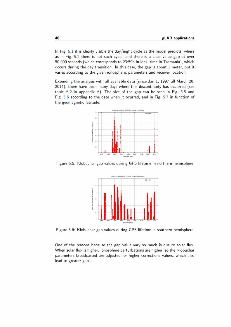
In Fig. 5.1 it is clearly visible the day/night cycle as the model predicts, whereas in Fig. 5.2 there is not such cycle, and there is a clear value gap at over50.000 seconds (which corresponds to 23:59h in local time in Tasmania), whichoccurs during the day transition. In this case, the gap is about 1 meter, but itvaries according to the given ionospheric parameters and receiver location.

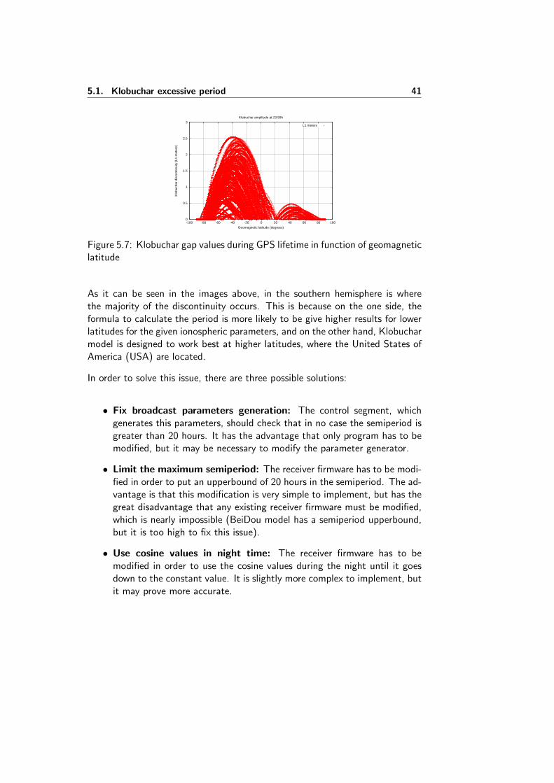
Extending the analysis with all available data (since Jan 1, 1997 till March 20,2014), there have been many days where this discontinuity has occurred (seetable A.2 in appendix A). The size of the gap can be seen in Fig. 5.5 andFig. 5.6 according to the date when it ocurred, and in Fig. 5.7 in function ofthe geomagnetic latitude.

0

0.2

0.4

0.6

0.8

1

1.2

1.4

1998 2000 2002 2004 2006 2008 2010 2012 2014

Klo

buch

ar d

isco

ntin

uity

(L1

met

ers)

Fractional years

Klobuchar amplitude at 23:59h in northern hemisfere

L1 meters

Figure 5.5: Klobuchar gap values during GPS lifetime in northern hemisphere

0

0.5

1

1.5

2

2.5

3

1998 2000 2002 2004 2006 2008 2010 2012 2014

Klo

buch

ar d

isco

ntin

uity

(L1

met

ers)

Fractional years

Klobuchar amplitude at 23:59h in southern hemisphere

L1 meters

Figure 5.6: Klobuchar gap values during GPS lifetime in southern hemisphere

One of the reasons because the gap value vary so much is due to solar flux.When solar flux is higher, ionosphere perturbations are higher, so the Klobucharparameters broadcasted are adjusted for higher corrections values, which alsolead to greater gaps.

5.1. Klobuchar excessive period 41

0

0.5

1

1.5

2

2.5

3

-100 -80 -60 -40 -20 0 20 40 60 80 100

Klo

buch

ar d

isco

ntin

uity

(L1

met

ers)

Geomagnetic latitude (degrees)

Klobuchar amplitude at 23:59h

L1 meters

Figure 5.7: Klobuchar gap values during GPS lifetime in function of geomagneticlatitude

As it can be seen in the images above, in the southern hemisphere is wherethe majority of the discontinuity occurs. This is because on the one side, theformula to calculate the period is more likely to be give higher results for lowerlatitudes for the given ionospheric parameters, and on the other hand, Klobucharmodel is designed to work best at higher latitudes, where the United States ofAmerica (USA) are located.

In order to solve this issue, there are three possible solutions:

• Fix broadcast parameters generation: The control segment, whichgenerates this parameters, should check that in no case the semiperiod isgreater than 20 hours. It has the advantage that only program has to bemodified, but it may be necessary to modify the parameter generator.

• Limit the maximum semiperiod: The receiver firmware has to be modi-fied in order to put an upperbound of 20 hours in the semiperiod. The ad-vantage is that this modification is very simple to implement, but has thegreat disadvantage that any existing receiver firmware must be modified,which is nearly impossible (BeiDou model has a semiperiod upperbound,but it is too high to fix this issue).

• Use cosine values in night time: The receiver firmware has to bemodified in order to use the cosine values during the night until it goesdown to the constant value. It is slightly more complex to implement, butit may prove more accurate.

42 gLAB applications

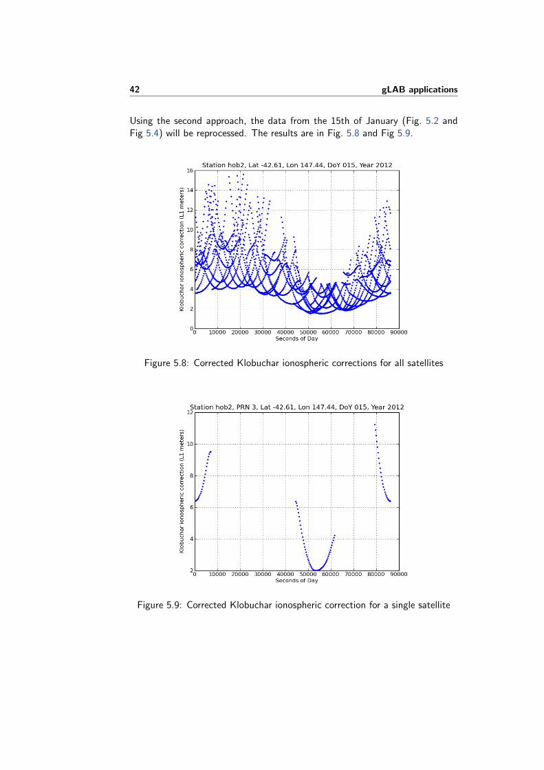
Using the second approach, the data from the 15th of January (Fig. 5.2 andFig 5.4) will be reprocessed. The results are in Fig. 5.8 and Fig 5.9.

Figure 5.8: Corrected Klobuchar ionospheric corrections for all satellites

Figure 5.9: Corrected Klobuchar ionospheric correction for a single satellite

5.1. Klobuchar excessive period 43

In Fig. 5.8, there is no value gap, and there is a clear stable period of 14.400seconds (4 hours), starting at about 51.000 seconds which corresponds to nighttime, as the Klobuchar model predicts. The length of four hours is due to thatthe semiperiod is 20 hours (which determined the length of the day), so theremaining time for one day are the 4 hours stated before.

As for Fig 5.9, there is also no gap, and the values computed are continuous.

Last, but not least, it is necessary to analyze how a semiperiod greater than 20hours affects user positioning. Thus, it will be compared, for each coordinate,how the error varies between using the nominal Klobuchar model and a correctedversion (using the second method for correction, setting the upperbound to 20hours).

In Fig. 5.10, Fig. 5.11 and Fig. 5.12 below are shown the error obtained in thethree coordinates for the nominal and corrected Klobuchar model, among theabsolute value of the difference between them:

Figure 5.10: Positioning error in north component between original and cor-rected Klobuchar model

44 gLAB applications

Figure 5.11: Positioning error in east component between original and correctedKlobuchar model

Figure 5.12: Positioning error in up component between original and correctedKlobuchar model

5.2. Ionospheric model comparison 45

It is clearly visible in all figures that around 50.000 seconds -where the discon-tinuity occurs- the difference between the models rises to about 1 meter. Inthe north and up component the corrected model has less error, but the eastcomponent has more error than the original, which shows that the correctedmodel may introduce additional error due to the modified semiperiod.

Although the gap size reaches about a meter, it is not critical, due to that userswho use Klobuchar model do simple positioning, where the error is about 5-10meters. As an example, in Fig. 5.10, Fig. 5.11 and Fig. 5.12, the total erroramount oscillates more than a meter, so it is impossible to distinguish if thesource of the error is from the Klobuchar model or the few accurate broadcastnavigation parameters for computing satellite position or clock drift.

5.2 Ionospheric model comparison

With gLAB capable of processing with multiple ionospheric models, this allowsto compare the performance of each model in terms of accuracy (how close isthe predicted value from the real one) and error positioning (how ionospheremodelling affects user positioning). In order to acquire precise results it shouldbe necessary to process data from many stations and days, but it is out of thescope for this project. Here it will only be provided a proof of concept, showingthe positioning error and RMS for a given day and station.

In the following figures the positioning error is presented for all models (exceptfor BeiDou, due to there were no ionospheric parameters available), with twomodes: using only code and using code plus carrier phase. The positioning erroris computed using precise orbits, clocks and single frequency. The reason to useprecise orbits is to take out the other meter error source, so the results directlyshow the performance of the ionosphere model.

(a) Klobuchar code (b) Klobuchar code and carrier

Figure 5.13: Positioning error with Klobuchar model

46 gLAB applications

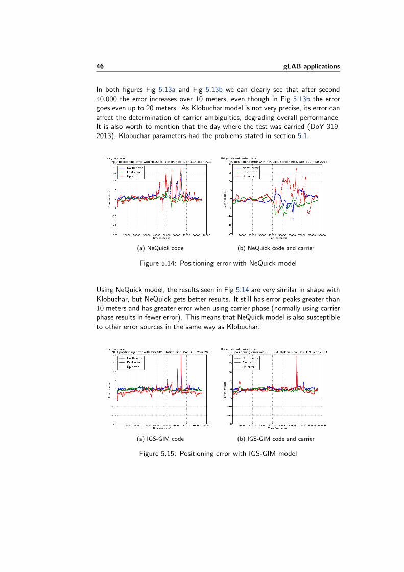
In both figures Fig 5.13a and Fig 5.13b we can clearly see that after second40.000 the error increases over 10 meters, even though in Fig 5.13b the errorgoes even up to 20 meters. As Klobuchar model is not very precise, its error canaffect the determination of carrier ambiguities, degrading overall performance.It is also worth to mention that the day where the test was carried (DoY 319,2013), Klobuchar parameters had the problems stated in section 5.1.

(a) NeQuick code (b) NeQuick code and carrier

Figure 5.14: Positioning error with NeQuick model

Using NeQuick model, the results seen in Fig 5.14 are very similar in shape withKlobuchar, but NeQuick gets better results. It still has error peaks greater than10 meters and has greater error when using carrier phase (normally using carrierphase results in fewer error). This means that NeQuick model is also susceptibleto other error sources in the same way as Klobuchar.

(a) IGS-GIM code (b) IGS-GIM code and carrier

Figure 5.15: Positioning error with IGS-GIM model

5.2. Ionospheric model comparison 47

IGS-GIM provides much better results as it can seen in Fig 5.15. The error isaround 3 meters, which is the expected for this model. With this model, usingcode and carrier gets better results, it can be clearly seen in Fig 5.15b, in whichthe error is smaller and less noiser than in Fig 5.15a. The error peaks can bedue to a rare ionospheric disturbance (as at this time the previous models alsohad error peaks) which the current model is unable to predict.

(a) F-PPP code (b) F-PPP code and carrier

Figure 5.16: Positioning error with F-PPP model

With F-PPP model, it can be seen in Fig 5.16 that the error is at the level of 1meter, with maximum error peaks of 3 meters. This proves that F-PPP is veryprecise and capable of following any ionospheric perturbation, due to that it hasno error peaks at about 62.000 seconds that appeared in the other models.

The RMS for each figure and the processing time (for the whole process, ingLAB) are in the following tables:

RMS Klobuchar NeQuick IGS−GIM F-PPPCode 83.35 63.66 43.02 2.09

Code +344.81 72.53 32.50 1.49

carrier phase

Table 5.1: RMS of 3D positioning error for station hofn, DoY 319, Year 2013

Processing time (s) /day Klobuchar NeQuick IGS−GIM F-PPPCode 1.65 4.75 1.71 12.04

Code +1.75 4.96 1.85 12.18

carrier phase

Table 5.2: Processing time of 3D positioning error for station hofn, DoY 319,Year 2013

48 gLAB applications

Moreover, in order to prove that the source of the positiong error showed aboveare due to the ionosphere model limitations, Klobuchar, NeQuick and IGS-GIMmodels will be compared with F-PPP model, the only one who was able to reach1 meter error without large error peaks. The results are in Fig 5.17:

(a) F-PPP only (b) F-PPP vs Klobuchar

(c) F-PPP vs NeQuick (d) F-PPP vs IGS-GIM

Figure 5.17: F-PPP vs ionospheric models

As it can be clearly seen in Fig 5.17, at 60.000 seconds there are peak valuesfor the ionospheric correction that only F-PPP is able to follow, therefore this isthe cause of the positioning error peaks seen at this time in Fig 5.13, Fig 5.14and in Fig 5.15.

With the results shown above, the best ionospheric model in terms of accuracyis, by far, F-PPP, but at the current state it has the longest processing timedue to the file format used, which is very far from using the minimum spaceas a IONEX does (now is about 100 times bigger than a IONEX file). Thedisadvantage of F-PPP and IGS-GIM is that they both need an external datafile, while Klobuchar and NeQuick only uses the parameters broadcasted in thenavigation message. Klobuchar also has the advantage to be the fastest, whichmakes it more suitable for mobile devices.

5.3. Other studies where gLAB has been used as a Data Processing Tool 49

5.3 Other studies where gLAB has been used as aData Processing Tool

In section 5.1 a study of Klobuchar periodicity has been with gLAB, while insection 5.2 a proof of concept of ionosphere comparisons with gLAB has beenmade. Additionaly, in two proceedings already published the new version ofgLAB has been used to compute some of the results presented in them.

In the proceedings [Juan et al., 2014b] and [Sanz et al., 2014] it was computedfor several months the ionospheric correction values for Klobuchar, NeQuick,IGS-GIM and F-PPP with gLAB, using these values to make a ionosphere per-formance comparison during a long period, a direct application shown in section5.2.

Also, in the in the proceeding [Vinh et al., 2013], the ionospheric correctionvalues for Klobuchar and IGS-GIM for the region it was studied in the paper(Vietnam) were computed using gLAB.

Last but not least, in the proceeding [Juan et al., 2014a], gLAB was used tocompute Klobuchar, NeQuick and IGS-GIM values for a period of about 6months.

Chapter 6

Conclusion

In this Final Degree Project it has been proven once again that gLAB is avery powerful tool for processing GNSS data. The main goal of the projectwas to include the ionospheric models described in chapter 3, validate thisimplementation with the test described in section 4.2 and provide some examplesof use for the new version of gLAB.

During the programming phase, it should be emphasised that the source codestructure and design of gLAB has proved to have a flexible and fully preparedfor updates, although being a source code with about 20.000 lines. Its modulardesign, with different files for the several parts of the processing (for example afile only for functions for reading files, another only for the filter, etc.), makesit much easier for any programmer to read -and update- the necessary parts.

In the test phase, the results obtained -with the test designed just for thispurpose-, proof that the results given by gLAB have the same accuracy up tolevel of 10−9, hence it can be said the values from gLAB are the same fromthe third party programs used as a reference. This test was done in a grid ofstations in all the world for several days, so the maximum number of possibilitieswere covered and the results were completely satisfactory.

Finally, in chapter 5, there are two examples of the direct use of gLAB, in section5.1 there was the Klobuchar period anomaly, which could be thoroughly studiedand tested a possible solution modifying the code (where as in proprietary formatwould not have been possible), and in 5.2 there was a proof of concept of thecapability for gLAB for being used to compare ionosphere models, which hasproved to be very useful, as it is the main use in the GNSS Meetings andWorkshop Proceedings stated in 5.3.

Appendix A

List of days with Klobuchardiscontinuity

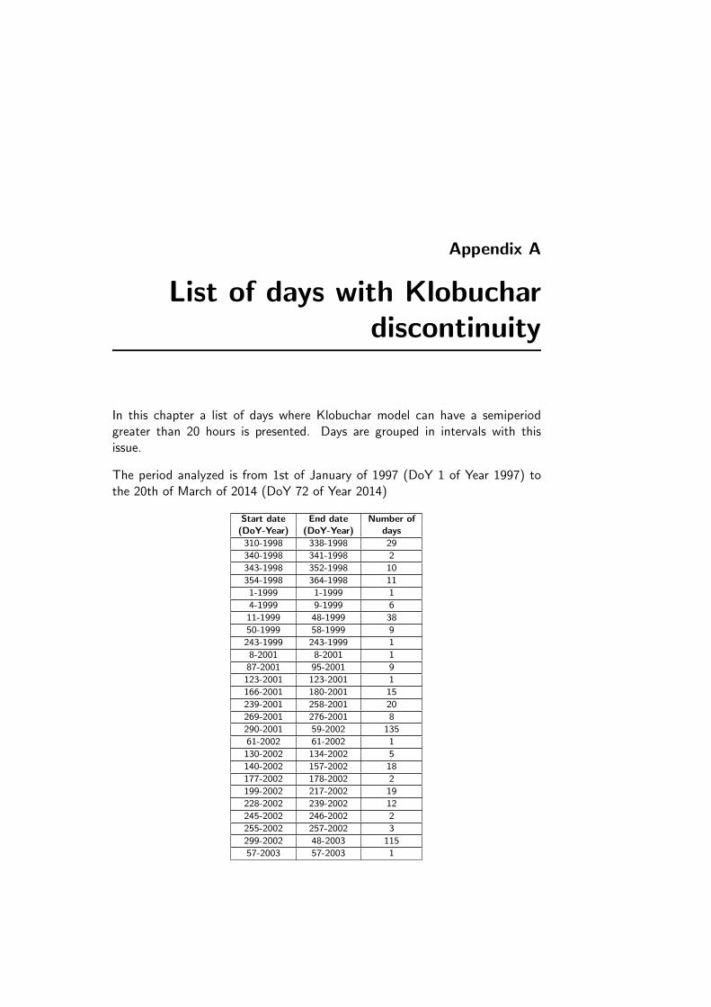
In this chapter a list of days where Klobuchar model can have a semiperiodgreater than 20 hours is presented. Days are grouped in intervals with thisissue.

The period analyzed is from 1st of January of 1997 (DoY 1 of Year 1997) tothe 20th of March of 2014 (DoY 72 of Year 2014)

Start date End date Number of(DoY-Year) (DoY-Year) days

310-1998 338-1998 29

340-1998 341-1998 2

343-1998 352-1998 10

354-1998 364-1998 11

1-1999 1-1999 1

4-1999 9-1999 6

11-1999 48-1999 38

50-1999 58-1999 9

243-1999 243-1999 1

8-2001 8-2001 1

87-2001 95-2001 9

123-2001 123-2001 1

166-2001 180-2001 15

239-2001 258-2001 20

269-2001 276-2001 8

290-2001 59-2002 135

61-2002 61-2002 1

130-2002 134-2002 5

140-2002 157-2002 18

177-2002 178-2002 2

199-2002 217-2002 19

228-2002 239-2002 12

245-2002 246-2002 2

255-2002 257-2002 3

299-2002 48-2003 115

57-2003 57-2003 1

54 Chapter A. List of days with Klobuchar discontinuity

166-2003 168-2003 3

303-2003 303-2003 1

305-2003 311-2003 7

328-2003 346-2003 19

349-2003 24-2004 41

36-2004 37-2004 2

202-2004 206-2004 5

308-2004 315-2004 8

319-2004 343-2004 25

348-2004 9-2005 28

16-2005 23-2005 8

319-2005 319-2005 1

321-2005 330-2005 10

336-2005 351-2005 16

356-2005 1-2006 11

320-2006 325-2006 6

340-2006 351-2006 12

3-2007 3-2007 1

7-2007 8-2007 2

346-2007 352-2007 7

322-2010 323-2010 2

322-2010 323-2010 2

342-2010 345-2010 4

347-2010 350-2010 4

3-2011 7-2011 5

309-2011 30-2012 87

32-2012 36-2012 5

186-2012 186-2012 1

189-2012 189-2012 1

192-2012 194-2012 3

196-2012 197-2012 2

317-2012 20-2013 70

36-2013 36-2013 1

303-2013 304-2013 2

311-2013 61-2014 116

Table A.1: List of days with Klobuchar discontinuity

In the following table there is a summary with the total number of days withdiscontinuity, and the percentage of these in the days processed.

Number of days Number ofPercentage

with discontinuity GPS days processedIn northern hemisphere 347 6289 5,52%

In southern hemisphere 888 6289 14,12%

In any latitude 1001 6289 15,92%

Table A.2: Percentage of days with Klobuchar discontinuity

Appendix B

Multi-platform arrangements

One of European Space Agency (ESA)’s requirements is that gLAB tool shouldbe multi-platform. gLAB was developed in Linux due to the powerful commandline shell available, which is perfect for scripting, fast data handling and massprocessing. In order to show these capabilities and how gLAB was designed tobe used, all the tutorials and exercises were prepared to be done under a Linuxenvironment. Therefore, in non Linux platforms it is necessary to add additionalsoftware so as the user experience is the same as in Linux.

B.1 Windows

There is an application for Windows called Cygwin (https://cygwin.com/),developed by RedHat and published under GPL license, which creates a Linuxshell in Windows. Their slogan is “Get that Linux feeling... in Windows” andthey got it. It has most of the programs that a Linux user uses, and it canrun Linux shell scripts straight out of the box. For our purposes, this allows touse all the training and exercises material for Linux to be run under Windowswithout modifications.

For an easy start for any user, an automatic installer (and uninstaller) for Cygwinhas been created and embedded in gLAB’s installer. The steps to do it are thefollowing:

• Retrieve Cygwin packages: Cygwin has a lot of packages, but only thenecessary ones will be installed in order to save disk and time.

56 Chapter B. Multi-platform arrangements

• Cygwin installer batch script: Create a batch script (our script is “InstallCygwin.bat”) for installing Cygwin which will receive as a parameter thegLAB installation path (from the installer). The script must be able towork with any language and Windows version. The steps in the script are:

� Call Cygwin installer in unattended mode, giving as parameters theinstallation path (in our case fixed to C:\Cygwin), and the list ofpackages to install.

� Retrieve the desktop and start menu path from the registry andcreate shortcuts

� Copy Cygwin uninstall script to a system path. It cannot be copiedto gLAB’s installation directory because the user must be able touninstall gLAB without uninstalling Cygwin or erasing our Cygwinuninstaller script.

� Copy bash user profiles to user’s home directory (this is optional, butit sets our aliases and colour configuration we like in Cygwin)

� Copy gLAB’s and graph execution scripts to Cygwin folder. Thisscripts are due to that gLAB and graph programs used are the Win-dows version, but in the exercises they will be called with linux paths,so these scripts automatically convert to Windows paths.

� Modify the scripts from the previous step in order to include in themthe path where gLAB is installed. In this case the installer called abash script (see items below).

• Cygwin uninstaller batch script: Create a batch script for uninstalling(the file is “Uninstall Cygwin.bat”). There is no official uninstaller forCygwin (only the instructions on the web page), so creating a script wasnecessary. It must be also able to work with any language and Windowsversion. The steps in the script are:

� Check for administrative privileges. If it is called from gLAB’s unin-staller it will inherit administrative privileges, but if it is called fromthe Start Menu it will not have them. It should prompt the user forprivileges if it has not got administrative privileges.

� Prompt the user to confirm if he wants to delete Cygwin. Thisallows the user to uninstall gLAB but not Cygwin, and also as aconfirmation in case the user did not want to call the uninstaller.

� Retrieve the desktop and start menu path from the registry anddelete shortcuts and user profiles files copied in the installation script.

� Delete Cygwin folder and Cygwin data in the Windows registry.

� Delete the uninstaller script file itself, so there is no files remainingin the computer.

B.2. Macintosh 57

• Cygwin configuration files: As mentioned in the Cygwin installer script,if the prompt shell is to be customized, the files .bashrc, .bash profile,.minttyrc and .vimrc have to be created and copied to the home folder.

• gLAB’s and graph execution scripts: As mentioned in the Cygwininstaller script, these execution scripts just read the input parameters andcheck for pathes. If a Linux path is found, it translates to Windowspaths. Afterwards they call the Windows gLAB or graph executables withthe given parameters (our file is “.run graph.sh”).

• Insert path in execution scripts: The execution script needs to knowwhere gLAB is installed, which a priori is not known. For this reason,during installation a bash script was created in order to to insert the pathin them (the file is “Configure cygwin.sh”). Additionally, this executionscripts were linked to the “/bin” folder, so they can be accessed from anydirectory.

• Modify gLAB’s installer script: gLAB’s installer is created with an InnoSetup script. It has to be modified so it includes the Cygwin installationfiles, copy them to a temporal folder (afterwards these files are no longerneeded), show the option to install Cygwin (using the installation script)after gLAB has installed and call the Cygwin uninstall script when unin-stalling.

All the previous steps require some scripting knowledge, in both Windows andLinux and it is out of the scope of this project to explain how to do them. Nev-ertheless, all scripts have plenty of comments and are included in the electroniccontent, so any user can make his own installer.

B.2 Macintosh

After several tests, it was not possible to make the GUI and the graph module towork under OSX due to python problems. Therefore, the solution for Macintoshis to create a virtual machine with VirtualBox, containing a light version ofUbuntu, with gLAB already installed. This allows any user in any platform todownload the virtual machine (shared in a standard “.ova” format), open it andstart working in a few minutes. The virtual machine files and the installationinstruction are available at gAGE’s website http://www.gage.es/gnss_book.

Appendix C

F-PPP v0.50

This is a preliminary unofficial version file for the F-PPP model. It has a headerwith the same pattern as the RINEX. Once the header ends, a data map startswith a list of hardware delays for each satellite (the order of the data is given inthe header, and each TEC may have their own hardware delays, so the last onefound should be used). Then a ionospheric map is given for a determinate regionand for a given epoch (every 5 minutes), ordered by longitude and latitude.The five fields in each line are: longitude, latitude, the partial Total ElectronContent (TEC), the sigma (mean error) and the map layer (the ionosphere isgiven in two layers).

(Continues in the next page)

0.5 IONOSPHERE MAPS FPPP FPPP VERSION / TYPE 2013 11 15 0 0 0 EPOCH OF FIRST MAP 300 INTERVAL 6371.0 BASE RADIUS 268.0 1600.0 HGT1 / HGT2 2.5 2.5 DLT / DLAT -90 90 MIN/MAX LAT TECUS MAP UNITS PRN FRAC_1 FRAC_W IFB(P1-P2) HARDWARE DELAYS cycles FRAC UNITS L1-L2 (LI) meters IFB UNITS END OF HEADER 1 START OF TEC MAPG 1 0.2529 0.1434 -4.320G 2 -0.2733 0.0176 1.201G 3 0.5647 0.5431 -1.847G 4 -0.6354 0.2289 -1.545G 5 0.7510 -0.4209 -0.836G 6 -0.1205 -0.2831 -1.750G 7 -0.0502 0.0081 -0.648G 8 -1.3232 0.4370 -1.903G 9 -0.1151 0.2681 -1.631G10 -0.2813 -0.2179 -2.269G11 -0.2955 0.3953 -0.459G12 0.5937 0.3640 -0.424G13 1.2399 -0.1631 -0.615G14 0.0338 0.0258 -0.962G15 0.1745 0.1818 -0.808G16 0.2792 0.1751 -0.768G17 0.0090 0.2541 -0.744G18 -0.0292 0.3420 -0.583G19 0.0732 0.1530 0.153G20 0.0634 -0.2927 -1.159G21 0.8965 -0.4240 -0.561G22 1.1177 -0.0109 0.681G23 0.5559 -0.0780 1.135G24 0.2802 -0.1223 -3.347G25 0.4423 -0.1454 -3.799G26 -0.3572 0.0590 -1.616G27 -0.3993 -0.3083 -3.100G28 -0.1628 0.4581 -0.696G29 -0.2691 0.0889 -0.968G31 0.0087 0.2139 -0.162G32 -0.3182 0.1141 -2.102 2013 11 15 0 0 0 EPOCH OF CURRENT MAP 0.0 -90.0 13.7238 1.43e+00 2 2.5 -90.0 13.6190 1.33e+00 2

5.0 -90.0 13.5047 1.24e+00 2 7.5 -90.0 13.4000 1.14e+00 2 10.0 -90.0 13.2857 1.05e+00 2 12.5 -90.0 13.1714 9.52e-01 2 15.0 -90.0 13.0666 9.04e-01 2 17.5 -90.0 12.9524 8.66e-01 2 20.0 -90.0 12.8476 8.37e-01 2 22.5 -90.0 12.7333 8.37e-01 2 25.0 -90.0 12.6190 8.56e-01 2... 355.0 90.0 4.2798 6.21e+01 1 355.0 90.0 4.5782 5.99e-01 2 357.5 90.0 4.0436 6.49e+01 1 357.5 90.0 4.5592 6.38e-01 2 2 START OF TEC MAPG 1 0.2426 0.1439 -4.320G 2 -0.2832 0.0175 1.202G 3 0.5537 0.5429 -1.847G 4 -0.6443 0.2294 -1.545G 5 0.7331 -0.4201 -0.836G 6 -0.1312 -0.2831 -1.749G 7 -0.0576 0.0081 -0.648G 8 -1.3331 0.4371 -1.903G 9 -0.1244 0.2683 -1.631G10 -0.2864 -0.2180 -2.268G11 -0.3059 0.3952 -0.459G12 0.5937 0.3640 -0.424G13 1.2203 -0.1641 -0.615G14 0.0244 0.0251 -0.963G15 0.1708 0.1817 -0.808G16 0.2723 0.1750 -0.768G17 0.0090 0.2541 -0.745G18 -0.0372 0.3417 -0.584G19 0.0620 0.1530 0.153G20 0.0565 -0.2925 -1.159G21 0.8867 -0.4242 -0.563G22 1.1336 -0.0178 0.681G23 0.5459 -0.0781 1.135G24 0.2712 -0.1229 -3.346G25 0.4386 -0.1471 -3.801G26 -0.3603 0.0590 -1.617G27 -0.4131 -0.3091 -3.100G28 -0.1725 0.4584 -0.695G29 -0.2774 0.0886 -0.967G31 999.0000 999.0000 -0.162G32 -0.3295 0.1140 -2.102 2013 11 15 0 5 0 EPOCH OF CURRENT MAP

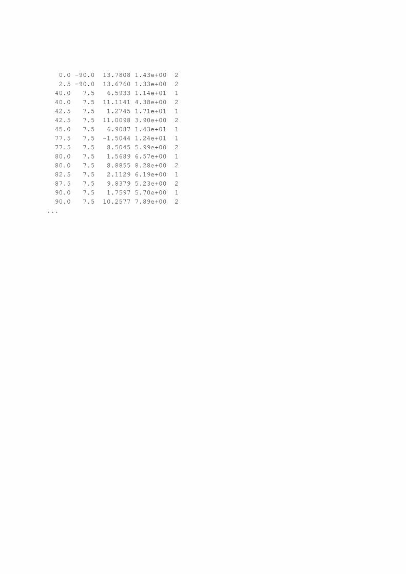
0.0 -90.0 13.7808 1.43e+00 2 2.5 -90.0 13.6760 1.33e+00 2 40.0 7.5 6.5933 1.14e+01 1 40.0 7.5 11.1141 4.38e+00 2 42.5 7.5 1.2745 1.71e+01 1 42.5 7.5 11.0098 3.90e+00 2 45.0 7.5 6.9087 1.43e+01 1 77.5 7.5 -1.5044 1.24e+01 1 77.5 7.5 8.5045 5.99e+00 2 80.0 7.5 1.5689 6.57e+00 1 80.0 7.5 8.8855 8.28e+00 2 82.5 7.5 2.1129 6.19e+00 1 87.5 7.5 9.8379 5.23e+00 2 90.0 7.5 1.7597 5.70e+00 1 90.0 7.5 10.2577 7.89e+00 2...

Acknowledgements

I would also like to thank my family for their patience and support during thistime.

I would like to specially thank my project director Dr. Jaume Sanz Subiranafor teaching me GNSS theory from scratch and his continuous help during therealisation and writing of this project.

I would like to thank Adria Rovira Garcia and Dr. Jose Miguel Juan Zornozafor their continuous support during all the project.

Last, but not least, thanks to Dr. Alberto Garcıa Rigo for his help when testingIONEX model in gLAB, while listening to my heavy metal music playlists.

Bibliography

[Arbesser-Rastburg, B., 2006] Arbesser-Rastburg, B., 2006. TheGalileo Single Frequency Ionospheric Correction Algorithm.http://sidc.oma.be/esww3/presentations/session4/arbesser.pdf.

[Di Giovanni and Radicella, 1990] Di Giovanni, G. and Radicella, S., 1990. AnAnalytical Model of the Electron Density Profile in the Ionosphere. Ad-vances in Space Research 10(11), pp. 27–30.

[Juan et al., 2014a] Juan, J., Sanz, J., Gonzalez-Casado, G., Rovira-Garcia, A.and Ibanez, D., 2014a. Accurate reference ionospheric model for testingGNSS ionospheric correction in EGNOS and Galileo.

[Juan et al., 2014b] Juan, J., Sanz, J., Rovira-Garcia, A., Gonzalez-Casado,G., Escudero Royo, M., Ibanez, D., Vinh, L. T. and Khoi, V., 2014b. AnAccurate Global Ionospheric Model for GNSS users.

[Klobuchar, 1987] Klobuchar, J., 1987. Ionospheric Time-Delay Algorithms forSingle-Frequency GPS Users. IEEE Transactions on Aerospace and Elec-tronic Systems AES-23(3), pp. 325–331.

[Montenbruck and Steigenberger, 2013] Montenbruck, O. and Steigenberger,P., 2013. The BeiDou Navigation Message. International Global Navi-gation Satellite Systems Society, IGNSS Symposium 2013 pp. 8–9.

[Rovira-Garcia et al., 2014] Rovira-Garcia, A., Juan, M. and Sanz, J., 2014. AReal-time World-wide Ionospheric Model for Single and Multi-frequencyPrecise Navigation. In: Proceedings of 27th International Technical Meet-ing of The Satellite Division of the Institute of Navigation, Tampa, Florida(USA).

[Sanz et al., 2013] Sanz, J., Juan, J. and Hernandez-Pajares, M., 2013. GNSSData Processing, Vol. I: Fundamentals and Algorithms. ESA Communica-tions, ESTEC. TM-23/1., Noordwijk, the Netherlands.

66 BIBLIOGRAPHY

[Sanz et al., 2014] Sanz, J., Rovira-Garcia, A., Juan, J., Gonzalez-Casado, G.,Ibanez, D. and Escudero, M., 2014. Fast-PPP on a planetary scale.

[Stefan Schaer, 1998] Stefan Schaer, W. G., 1998. IONEX: The IONosphereMap EXchange Format Version 1. In: Proc. of the IGS Analysis CenterWorkshop., Darmstadt, Germany.

[Vinh et al., 2013] Vinh, L., Quang, P. X., Garcia-Rigo, A., Rovira-Garcia, A.and Ibanez Segura, D., 2013. Experiments on the Ionospheric Models inGNSS. In: Proceedings of 20th Asia-Pacific Regional Space Agency Forum,Vol. 113number 335, Hanoi, Vietnam.