1

IMPLEMENTATION OF THE LRFD GEOTECHNICAL STRENGTH LIMIT STATE FOR COMPRESSION RESISTANCE

OF A SINGLE DRIVEN PILE

By:

Naser M. Abu-Hejleh, Ph.D., P.E (Corresponding Author) Geotechnical Engineering Specialist

FHWA Resource Center 4749 Lincoln Mall Drive, Suite 600, Matteson, IL 60443

Ph. 708-283-3550; Fax: 708 283 3550; E-mail: naser.abu-Hejleh@dot.gov

William Kramer, P.E. Foundations and Geotechnical Unit Chief

Bureau of Bridges and Structures, Illinois Department of Transportation Ph. (217) 782-7773, E-mail: William.Kramer@illinois.gov

Khalid Mohamed, PE., PMP

Principal Bridge Engineer - Geotechnical FHWA Headquarter, Washington, DC

Ph: 202-366-0886; Email: Khalid.mohamed@dot.gov

James H. Long Emeritus Faculty

Department of Civil Engineering, University of Illinois (217) 333-2543; E-mail: jhlong@illinois.edu

Mir A. Zaheer, P.E.

Geotechnical Design Engineer Office of Geotechnical Services, Indiana Department of Transportation

Ph. (317) 610 7251 Ext. 224; E-mail: mzaheer@indot.in.gov

Submitted to: 94th th Transportation Research Board Annual Meeting

Washington, D.C.

No. of text words = 6200 No. of Figures (4) x 250 words/Figure = 1000

No. of Tables (1) x 250 words/table = 250 Total number of words = 7450

1

ABSTRACT 1 2 This paper addresses issues and problems facing State DOTs in the development of LRFD design 3 specifications for driven piles based on the 2012 AASHTO LRFD Bridge Design Specifications. 4 It describes with solved example the design procedure to address the geotechnical strength limit 5 state for compression resistance of a single driven pile. Both the static analysis methods (e.g., 6 β-method) and field analysis methods (e.g., dynamic formulas) are used to determine the pile’s 7 nominal bearing resistances at various depths and the pile length. A new procedure is presented 8 to improve the agreement between the pile length estimated in the design and the pile length 9 finalized in the field. The effect of downdrag in the LRFD design of driven piles is discussed. 10 The use of setup, static load tests, and static analysis methods to finalize the pile lengths in the 11 LRFD design are described and their advantages are demonstrated. The results obtained from 12 addressing the geotechnical strength limit state are summarized in a design chart that can be used 13 by the foundation designers to optimize and finalize the LRFD design by determining the design 14 pile length and required field bearing resistance. Finally, a comprehensive LRFD Design 15 Example is solved to demonstrate the development and applications of design charts using a 16 static and three field analysis methods. 17 18 OVERVIEW 19 20 FHWA recently developed a new NHI training Course Number 132083, “Implementation of 21 LRFD Geotechnical Design for Bridge Foundations” (Abu-Hejleh et al., 2010). The goal of this 22 course is to assist State DOTs in the successful development of LRFD design specifications for 23 bridge foundations based on AASHTO LRFD Bridge Design Specifications (AASHTO, 2012) 24 and their local experiences. In these specifications, the geotechnical strength limit state for 25 compression resistance of a single driven pile is addressed by using both the static analysis 26 methods (e.g., α-method) and field analysis methods (e.g., wave equation analysis) to determine 27 the pile nominal bearing resistances at various depths and the pile length. Many of the LRFD 28 implementation questions received by FHWA from State DOTs have been related to the LRFD 29 design of driven piles. Some of these questions are addressed in the NHI Course Number 30 132083. However, there is a still a need to clarify the AASHTO LRFD geotechnical strength 31 limit state for compression resistance of a single driven pile and address following issues in 32 applying this limit state: 33 1. Large differences between the pile length estimated in the design using static analysis 34

methods and the pile length finalized and verified in the field using field analysis methods. 35 Contractors are often forced to order pile lengths based on pile lengths estimated in the 36 design phase before project construction begins, and before verification of pile bearing 37 resistance in the field, so as to meet rolling schedules and construction deadlines. Differences 38 between estimated and finalized pile lengths can be significant and lead to major construction 39 problems and delays in highway projects. 40

2. Evaluation and consideration of site-specific setup in LRFD design. Setup is common and 41 often results in large increases in pile geotechnical resistances that are not routinely 42 considered by most State DOTs in the design 43

3. Evaluation and consideration of downdrag effect in the LRFD design 44

2

4. Consideration and advantages of using static analysis methods to finalize the pile length in 1 the design phase. With this use, piles are driven in the field to a certain depth not to a certain 2 bearing resistance verified with a field analysis method. 3

5. Consideration of static load tests in the LRFD design and demonstration of their advantages. 4 5

This paper is developed to address these five issues. The paper describes with a solved example 6 the design procedures to address the geotechnical strength limit state for compression resistance 7 of a single driven pile. The results obtained from addressing the geotechnical strength limit state 8 are summarized in a design chart that can be used by the foundation designers to optimize and 9 finalize the LRFD design by determining the design pile length and required field bearing 10 resistance. Finally, the paper solves a comprehensive LRFD Design Example problem to 11 demonstrate the development and applications of the design charts using a static and three field 12 analysis methods. 13 14 2012 AASHTO LRFD Bridge Design Specifications to Determine Driven Pile Length 15 16 AASHTO Article 10.5.5 and Article 10.7 present the design specifications for a single and a 17 group of driven piles at all limit states. The pile length, L, is often finalized based on the LRFD 18 geotechnical strength limit state or extreme event limit state for compression resistance of a 19 single pile. The two limit states require the determination of the pile nominal bearing (or 20 geotechnical axial compression) resistances of a single pile at various depths. AASHTO Article 21 10.7.3.8 discusses two types of methods to determine the pile bearing resistance and pile lengths, 22 static and field analysis methods: 23 24 • Static analysis methods (β- and α- and Nordlund methods). According to AASHTO, these 25

methods are commonly used for estimating pile quantities in the design phase and may be 26 used to finalize pile length, L, in certain cases where field analysis methods are unsuitable for 27 field verification of nominal pile bearing resistance. Examples include projects with small 28 pile quantities or loads, and sites with long setup time (e.g., soft silts or clays (Article 29 10.7.3.8.6a). The FHWA manual on driven piles (Hannigan et. al., 2006) reported that using 30 the dynamic analysis methods (e.g., wave equation or dynamic formula) to verify the bearing 31 resistance of a friction H-pile in granular soils and finalize its length can be problematic and 32 result in significant length overruns. Such problems were reported by some State DOTs in 33 highway projects, where it was decided to either consider static load tests or static analysis 34 methods to finalize the pile length. According to the FHWA LRFD Implementation Manual 35 (Abu-Hejleh et. al., 2010), the static analysis methods can be used in all cases to finalize the 36 pile length as long as site variability is addressed in the design. Use and advantages of static 37 analysis methods to finalize pile length in the design phase will be demonstrated in this 38 paper. 39

40 • Field analysis methods. These methods are the static load test and the dynamic analysis 41

methods that include dynamic testing with signal matching, wave equation analysis, and 42 dynamic formulas. These methods are routinely used by the vast majority of State DOTs to 43 verify pile bearing resistances and finalize the pile length in the field. The design results with 44 these methods are: 45 • The required bearing resistance needed to finalize pile length in the field (AASHTO 46

3

Article 10.7.7). The geotechnical strength and extreme event limit states must be met in 1 the field by driving the pile to a length or depth where the required field bearing 2 resistance is achieved or exceeded. 3

• An estimate of the pile length, L, needed to achieve the required field bearing resistance 4 (Article 10.7.3.3). This pile length could be different from the pile length determined in 5 the field. The main reason for this difference is that the pile bearing resistances from the 6 field analysis methods are not available in the design, so static analysis resistances are 7 used to estimate the pile length, L. The paper presents a new procedure of estimating the 8 pile bearing resistances from the field analysis methods in the design phase that will 9 improve the agreement between the pile lengths estimated in the design and finalized in 10 the field. 11

12 In the design, obtain the pile lengths, L, and required field bearing resistances that are needed to 13 address both the strength limit and extreme event limit states for compression resistance of a 14 single pile. Then, consider the larger values of bearing resistances and pile lengths in the final 15 design (AASHTO Article 10.7.3.3). 16 17 The minimum pile length, Lm, referred to as the “minimum pile penetration” in AASHTO LRFD 18 Bridge Design Specifications, is defined as the deepest depth needed to meet all of the applicable 19 limit states and design requirements listed in AASHTO LRFD Article 10.7.6. These limit states 20 include the service limit states, lateral and uplift resistances of a single pile, and all limit states 21 for a group of piles. 22 23 The contract pile length, Lc, is the length developed in the design to address all applicable LRFD 24 design limit states for driven piles (Lc is the larger of L or Lm). If a static analysis method is 25 selected to finalize the pile length, the contract pile length represents the length the piles need to 26 be driven to in the field, since there will be no verification of pile bearing resistance in the field. 27 This length is the basis for the ordered length for production piles. With the field analysis 28 methods, there are two types of pile lengths: 29 • Contract pile length. This length is determined as described above. According to AASHTO 30

LRFD Bridge Design Specifications Articles 10.7.3.3 and 10.7.3.1, the contract pile length is 31 an estimate of the required pile quantities and should be used only as a basis for bidding, not 32 for ordering piles. 33

• Ordered pile length for production piles. This length is determined in the field as the 34 length needed to achieve both the: 35 • Required field bearing resistance needed to address the strength and extreme event limit 36

states for the axial compression resistances of a single pile, and the 37 • Minimum pile length, Lm, needed to address all other limit states (AASHTO LRFD 38

Article 10.7.9). 39 40

Based on AASHTO LRFD Articles 10.7.8 and 10.7.3, drivability analysis should be performed 41 in the design stage to ensure that piles can be driven in the field without damage to the required 42 bearing resistance or length (e.g., Lc or Lm) specified in the design. 43 44

4

This paper focuses only on addressing the LRFD geotechnical strength for compression 1 resistance of a single pile. Future publications should address other limit states and the 2 drivability analysis. 3 4 GEOTECHNICAL STRENGTH LIMIT STATE FOR THE AXIAL COMPRESSION 5 RESISTANCE OF A SINGLE PILE 6 7 Downdrag Effect and Total Factored Compression Load 8 9 According to the AASHTO LRFD Bridge Design Specifications, downdrag (DD) effects for the 10 design of a single driven pile at all limit states should be applied twice: as an additional 11 compression load and as an additional lost nominal geotechnical resistance (AASHTO Articles 12 3.11.8, 10.7.1.6.2, and 10.7.3.7). According to AASHTO LRFD, downdrag loads and resistances 13 at the strength limit state are the same and equal to the nominal geotechnical side resistances of 14 the soil layers located in and above the lowest layer contributing to downdrag. Hence, the total 15 factored axial compression load for a pile is 16 17

Qf + γp DD (1) 18 19 Where Qf is the largest factored axial compression load applied to the top of a single pile in a pile 20 group, DD is the downdrag load, and γp is its load factor, which is a function of the method 21 selected to determine the side resistance (see Table 3.4.1-2 in AASHTO LRFD). 22 23 In this paper, the 2012 AASHTO LRFD Bridge Design Specifications procedure to compute DD 24 loads and resistances at the strength state limit is used. However, it is recommended to develop a 25 complete settlement vs. axial compression load curve for a single pile up to the pile nominal 26 bearing resistance. Then, based on the relative settlement between the settling soil around the 27 pile and the pile at various limit states, evaluate the downdrag effect at various limit states. 28 29 Governing Equation and Design Chart for the Strength Limit State 30 31 The governing equation is: 32

33 Qf + γp DD ≤ φ Rn (2) 34

35 Where, Rn is the pile nominal bearing resistance of a single pile, and φ is the geotechnical 36 resistance factor for the method employed to determine Rn. For static analysis methods Rn = Rnstat 37 and φ = φstat and for field analysis methods, Rn = Rnfield and φ = φdyn. 38 39 Equation 2 can be written as: 40 41

Qf ≤ φ Rn – γpDD (3) 42 After the available Rn is determined at various depths using static and field analysis methods, the 43 factored nominal bearing resistance (RR) at various depths can be computed as: 44 45

5

RR = φ Rn (4) 1 The net factored nominal bearing resistance (RR-NET) at various depths is computed as: 2 3

RR-NET = φ Rn – γpDD (5) 4 By equating the applied factored loads, Qf, to RR-NET as 5

RR-NET = Qf = φ Rn – γpDD

(6)

6 a Qf vs. depth curve can be developed in the design chart and used to estimate the required pile 7 length, L, as the depth where RR-NET = Qf. The pile length, L, can also be determined at the depth 8 where the Rn resistance is equal to the required Rn resistance computed as: 9

10 Required Rn = (Qf + γpDD)/φ (7)

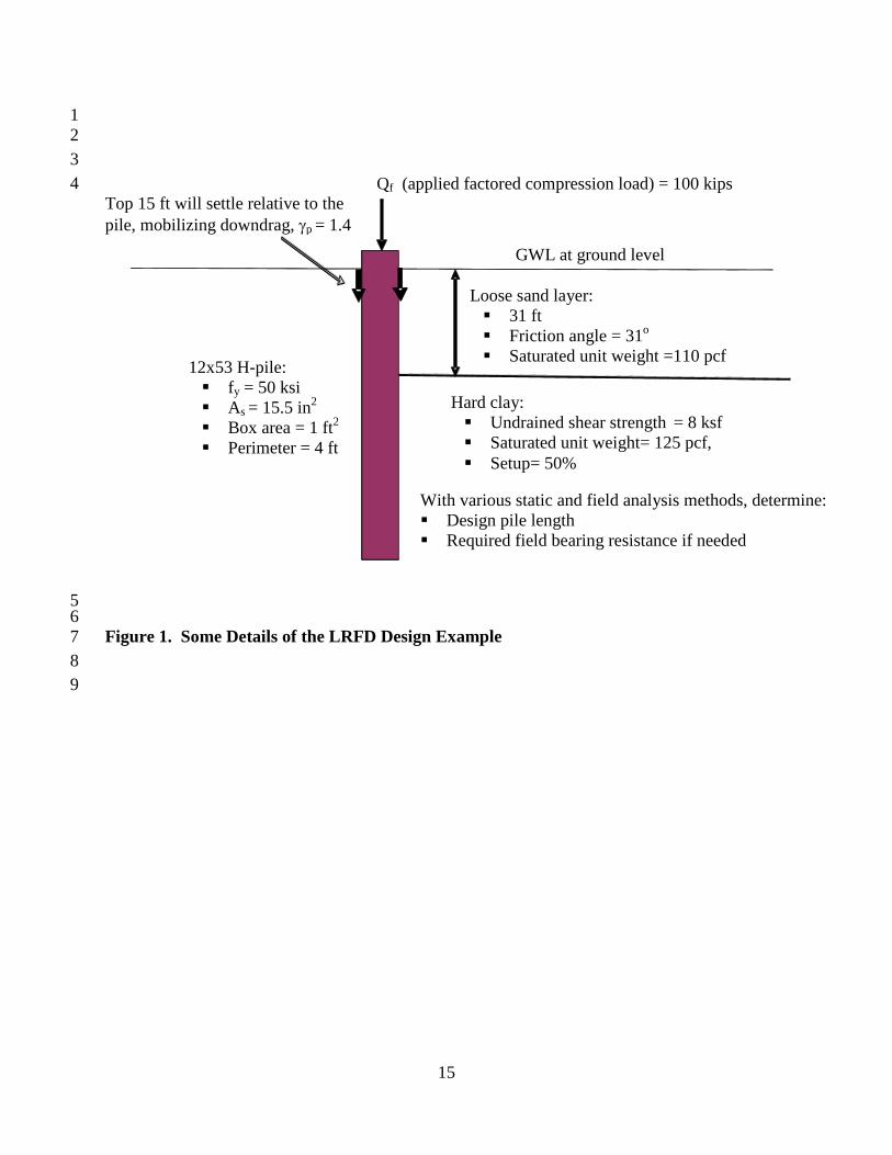
11 The design charts also include curves for the bearing resistances at various depths that can also 12 be used to determine the required bearing resistances. 13 14 As will be demonstrated later in this paper, the design charts provides the designer with a simple 15 and flexible approach to determining pile length, L, and required bearing resistance, especially 16 with continuous changes in the applied Qf loads during design. 17 18 LRFD DESIGN EXAMPLE PROBLEM 19 20 Some details of this example are given in Figure 1. As described in Figure 1, there are two soil 21 layers: loose silty sand layer with no setup that extends to a depth of 31 ft from the ground 22 surface, underlain by hard overconsolidated clay layer with an estimated setup factor of 50 23 percent (%). The top 15 ft of the loose silty sand layer will settle sufficiently to mobilize 24 downdrag. The load factor for the downdrag load, γp, at the strength limit state is given as 1.4. 25 The pile type is a 12x53 H-pile with steel yield strength, fy, of 50 ksi; steel area, As, of 15.5 in2; 26 box area of 1 ft2; and a box perimeter of 4 ft. It is required to develop design charts to address the 27 geotechnical strength limit state for compression resistance of a single pile using the following 28 four AASHTO LRFD design methods: 29 1. β-method, which is a static analysis method with a resistance factor, φ, of 0.25. 30 2. Wave equation analysis at end of driving (EOD) conditions with φ =0.5. 31 3. Wave equation analysis at beginning of restrike (BOR) conditions with φ =0.5. 32 4. Axial compression static load test with φ = 0.75. 33 34 It is also required to use the design charts to determine the pile length, L, and required field 35 bearing resistances (if needed) for an applied factored compression load of 100 kips. 36 37 38 39 40 41

6

NOMINAL BEARING RESISTANCES OF A SINGLE PILE 1 2

Types of Pile Bearing Resistances: 3 4 • Resistance mobilized during pile driving until the end of driving (EOD), Rndr. 5 • Short-term resistance, Rnre. This is the resistance that is developed shortly after pile driving. 6

The Rnre includes the permanent changes in the pile’s geotechnical resistances that occur after 7 EOD, for example due to setup and relaxation. Soil setup, expressed as a percentage, is 8 defined as 100(Rnre – Rndr)/Rndr. 9

• Long-term resistance (Rn). This is the resistance needed in LRFD design (Eq. 2). It is defined 10 as the minimum pile bearing resistance that would always be available to support the applied 11 loads during the entire design life of the foundation or design life of the structure supported 12 by the foundation, for example a bridge. Rn does not include the geotechnical resistance 13 losses (GL) that may not be available during the foundation design life. At the strength limit 14 state, GL can be generated from downdrag, scour, and future increases of the groundwater 15 level (GWL). 16

17 Bearing Resistances from Static Analysis Methods 18

19 The analytical expressions for these methods (e.g., Nordlund method for driven piles) require 20 deign soil and rock properties (e.g., undrained shear strength, Su) obtained from the subsurface 21 investigation (in-situ and laboratory testing). The bearing resistances are determined in the 22 following order: 23 24 • Rnre (Short Term Resistance). This includes the side and base resistances of all the soil 25

layers around the pile, including contributions from those layers that could eventually 26 contribute to geotechnical resistance losses (e.g., due to downdrag). 27

• Rndr (Resistance at End of Driving). This is estimated from Rnre and the given time-28 dependent changes in resistance after driving. For example, Rndr = Rnre/(1 + setup) if setup is 29 expected, and Rndr = Rnre if there is no setup. Site-specific setup factors are needed to develop 30 accurate Rndr resistances. 31

32 Use the GWL expected during pile driving in the estimation of Rnre and Rndr. 33

34 • Rn or Rnstat (Long-term Resistance). This resistance is determined using the same 35

procedure used to compute Rnre and the following guidelines: (a) use the highest GWL 36 expected during the design life of the foundation (b) subtract the geotechnical resistance 37 losses (GL). 38 • Downdrag (DD) Effect (AASHTO LRFD Articles 10.7.3.7 and 3.11.8). Assume zero 39

bearing resistance (Rnstat = 0) for the soil layers located in and above the lowest soil layer 40 contributing to downdrag. GL is the nominal side geotechnical resistances of these soil 41 layers (equal to DD load). For the soil layers located below the lowest soil layer 42 contributing to downdrag, Rnstat= Rnre – GL. 43

• Scour Effect (AASHTO LRFD Articles 3.7.5, 2.6.4.2, and 10.7.3.6). For estimation of 44 the total scour depth, Dscour, of a single pile at the strength limit state, consider Hannigan 45 et al. (2006) and the FHWA’s recently published Hydraulic Engineering Circular No. 18 46

7

(HEC-18) (Arneson et al., 2012). In computing Rn, consider the consequences of removal 1 of soil layers within the scour depth: 2 • Assume zero bearing resistance (Rnstat = 0) for all soil layers within the total scour 3

depth, Dscour. 4 • For the soil layers located below Dscour, compute Rnstat assuming no soil layers present 5

above them. Consider zero vertical effective stress only within the portion of the 6 scour depth subject to degradation and contraction, but not within the lower portion 7 generated from local scour (Hannigan et. al., 2006). 8

• GL due to scour is computed at various depths as Rnre – Rnstat. Use the expected depth 9 at the bottom of the pile to estimate GL due to scour. 10

11 The soil at any given depth can only contribute to losses due to either downdrag or scour, 12 but not both. If both scour and downdrag are possible during the design life, consider 13 them separately in the design to determine which controls the design (or pile length). 14

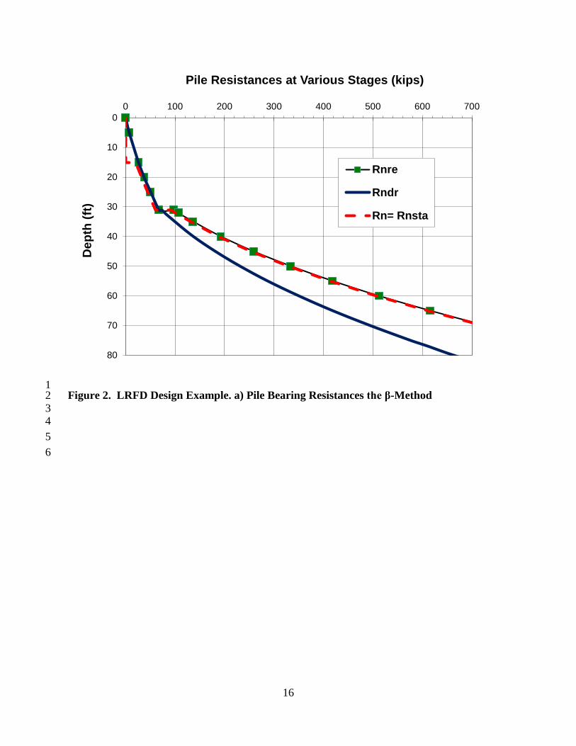
15 LRFD Design Example. Figure 2a shows the results of the available pile bearing resistances 16 (Rnre, Rnstat, and Rndr) at various depths using the β-method. These results are obtained as follows: 17 18 1. Develop the Rnre vs. depth profile as follows: 19

• The unit side resistance at various depths is computed as: 20 • 0.28σ’v in the sand layer, where σ’v is the vertical effective stress. 21 • 1.5 σ’v in the clay layer. 22

• The unit base resistance is computed as: 23 • 28σ’v in the sand layer. 24 • 9Su or 72 ksf in the clay layer, where Su is the undrained shear strength (8 ksf). 25

• The total side resistance in the top 15 ft is computed as 6 kips, so GL = DD = 6 kips. 26 2. Then, develop the Rndr profile as follows: 27

• In the sand layer, Rndr = Rnre, since no setup is considered for this layer. 28 • In the clay layer, Rndr < Rnre due to a setup of 50%. The Rnre unit side resistances in 29

the clay layer, computed at various depths as 1.5 σ’v, are divided by 1.5 to estimate 30 the Rndr unit resistances in the clay layers at various depths. The Rndr unit base 31 resistance is taken as 72 ksf with an assumption that setup does not affect base 32 resistance. 33

3. Finally, the Rn or Rnstat profile is developed as follows: 34 • Zero in the top 15 ft, and 35 • Rnre – 6 kips below the 15 ft depth. 36

37 Bearing Resistances from the Field Analysis Methods 38 39 AASHTO LRFD presents two types of methods to determine the pile nominal bearing resistance 40 in the field: 41 42 • Dynamic Analysis Methods (AASHTO LRFD Article 10.7.3.8.3-5). These methods include 43

dynamic testing with signal matching, wave equation analysis, and dynamic formulas. These 44 methods have two main components: an analytical model and the driving information needed 45

8

as input for the analytical model. This information includes the hammer-developed energy, 1 the hammer efficiency, and the penetration resistance. The penetration resistance is defined 2 as the number of hammer blows needed to drive the pile 1 inch. These methods can be used 3 to determine the nominal bearing resistances in the field during pile driving, at the end of 4 driving (EOD), Rndr, and at beginning of redrive (BOR), Rnre, by restriking the pile. The time 5 interval from EOD to BOR is called the restrike time. AASHTO LRFD (2012) provides 6 recommendations for restrike times for various types of soils. 7

• Static Load Test. In this method, the short-term nominal bearing resistance, Rnre, is 8 measured directly in the field after a waiting time following EOD, called “load test time.” 9 AASHTO LRFD (2012) recommends a minimum of 5 days for load test times. If restrike is 10 considered, perform it before conducting the static load tests. 11

12 This paper focuses only on soil setup (not relaxation). Setup is common and often results in large 13 increases in geotechnical resistances that are not routinely considered by most DOTs in the 14 design. To consider setup in design with the field analysis methods, the setup should be verified 15 by measurements of Rnre resistances from restrikes or load test. 16 17 With the field analysis methods, there are two options to determine bearing resistances and 18 finalize pile length: 19 20 • EOD Conditions, where only Rndr resistances are measured during driving and at EOD. 21

Site-specific setup is not needed and should not be directly considered in the design since it 22 will not be verified in the field. With this option, Rn is determined as: 23

24 Rn = Rnfield = Rndr – GL (8) 25

26 Based on Eqs. 7 and 8, the required Rndr is determined as: 27

28 29

Required Rndr = (Qf + γpDD)/φdyn + GL (9) 30 31

• BOR conditions, where both Rndr and Rnre resistances are measured. Site-specific setup 32 should be considered in the design since it will be verified in the field. With this option, Rn is 33 determined as: 34

35 Rn = Rnfield = Rnre – GL (10) 36 37

Based on Eqs. 7 and 10, the required Rnre is determined as: 38 39

Required Rnre = (Qf + γpDD)/φdyn + GL (11) 40 41

Based on the site-specific setup considered in the design, the required Rndr for BOR conditions 42 can be estimated as will be demonstrated later. 43

44 45 46

9

Estimation of the Bearing Resistances of the Field Analysis Methods during Design 1 2 The field analysis methods do not provide the Rnfield resistances needed for the estimation of the 3 pile length, L, in the design phase. AASHTO LRFD Equation C10.7.3.3.-1 suggests using the 4 resistance factor for the static analysis method, φstat, with Rnstat to estimate the pile length for the 5 field methods. This may lead to differences between the pile length estimated in the design and 6 the pile length finalized in the field using Rnfield and φdyn. Some State DOTs employ an 7 oversimplified approach of combining the φdyn from the field analysis method with the Rnstat 8 estimated from the static analysis method (factored bearing resistance = φdyn Rnstat) to estimate the 9 pile length. This is not theoretically accurate since the resistance factor from the field method is 10 matched with the resistance predictions from the static analysis method. To estimate the Rnfield 11 resistances, AASHTO LRFD (2012) recommends adjusting the static analysis resistance 12 predictions using bias in the resistance between the field and static analysis methods. However, 13 AASHTO does not provide a specific procedure for implementing this adjustment. The 14 following relationship is suggested to predict more accurately the resistances for a field analysis 15 method, Rnfield, from the resistances calculated with a static analysis method, Rnstat: 16

17 Rnfield = α Rnstat (12) 18 19 Where α is the resistance median bias between the field analysis method and the static analysis 20 method. This bias factor is expanded to αBOR at BOR conditions defined as: 21 22

αBOR = Rnre (field analysis method)/Rnre (static analysis method) (13) 23 24 The bias factor at EOD conditions, αEOD, is defined as: 25 26 αEOD = Rndr (field analysis method)/Rnre (static analysis method) (14) 27 28 With EOD conditions, only Rndr resistances will be measured in the field and only Rnre 29 resistances can be obtained from the static analysis methods because setup will not be directly 30 considered in the design or verified in the field. Therefore, αEOD is defined to estimate the Rndr 31 for the field analysis method from the Rnre calculated with the static analysis method. In this 32 case, αEOD accounts for both the resistance bias between the field and static analysis methods and 33 setup. 34 35 The αBOR and αEOD bias factors are used to estimate the resistances for a selected field analysis 36 method in the design phase using the resistances estimated from a selected static analysis method 37 as follows: 38 • BOR Conditions. Estimate Rndr, Rnre, Rnstat, and GL at various depths using the selected 39

static analysis method and multiply them by αBOR to predict at various depths the Rndr, Rnre, 40 Rnfield, and GL, respectively, for the selected field analysis method. 41

• EOD Conditions. Estimate Rnre, Rnstat, and GL at various depths using the selected static 42 analysis method and multiply them by αEOD to predict at various depths the Rndr, Rnfield, and 43 GL, respectively, for the selected field analysis method. 44

45

10

Then, use the estimated resistances of the field analysis methods to predict the pile length as will 1 be demonstrated later. 2 3 Determination of αBOR, αEOD, and Setup Factors 4 5 Accurate estimates of these parameters are needed to develop accurate estimates of the field pile 6 bearing resistances and length in the design phase. Two approaches are recommended to develop 7 these factors: 8 9 1. Local Calibration. This calibration can be performed as illustrated in Table 1 by compiling 10

the predicted Rnre resistances from the calibrated static analysis method and the measured 11 Rnre and Rndr resistances from the calibrated field analysis method at EOD and BOR 12 conditions. Analyze these data to obtain the resistance bias between the static analysis 13 method and the field analysis method at BOR conditions and at EOD conditions. Then, 14 obtain the resistance median bias factors at BOR conditions, αBOR, and at EOD conditions, 15 αEOD. A similar procedure (also show in Table 1) can be used to obtain the median setup 16 factor. Develop αBOR, αEOD, and the setup factor for different combinations of the typical 17 and local conditions encountered in the design and construction of production piles in actual 18 projects. For example, develop these factors for an H-pile driven into sand, using the β-19 method as the static analysis method and wave equation analysis as the field analysis 20 method, a specific driving system, and a specified restrike time and procedure. 21 22

2. Reliability Calibration Results. αBOR can be estimated based on the resistance mean bias, 23 λ, developed in the reliability calibration of resistance factors (Abu-Hejleh et al., 2010) for 24 the static analysis method, λstat, and for the field analysis method at BOR conditions, λBOR, 25 using the equation: 26

27 αBOR = λstat/λBOR (15) 28

29 Then, based on the expected site-specific setup factors, estimate αEOD as αBOR/(1 + setup). 30 Note that in this approach, αBOR and αEOD represent the mean (not median) resistance bias 31 factors, so they are approximate solutions. It is important to select λstat and λBOR parameters 32 that are representative of the typical local conditions encountered in the design and 33 construction of production piles in actual projects. 34

35 There are uncertainties it the procedure suggested above for estimating pile bearing resistances 36 that will be used to estimate pile length. Consequences of underestimating pile length are 37 typically greater than overestimating pile length. Based on these consequences and the 38 confidence in the developed αBOR, αEOD factors, it is recommended to apply an appropriate safety 39 factor to the estimated pile length. 40 41 LRFD Design Example. The resistances for the wave equation analysis at EOD and BOR 42 conditions presented in Figure 2b are developed as follows: 43 44

11

1. For both the sand and clay layers, αBOR is estimated as 0.61/1.05 = 0.58 based on λstat = 0.61 1 reported for the β-method (Paikowsky et al., 2004) and λBOR = 1.05 reported for wave 2 equation analysis (Smith et al., 2010). 3

2. With αBOR = 0.58 for both the sand and clay soils, αEOD is estimated as 0.58 for the sand (no 4 setup) and as 0.58/(1 + 0.5) = 0.39 for the clay layer (setup of 50%). 5

3. Multiply the Rndr, Rnre, and Rnstat resistances estimated from the β-method (Figure 2a) by 6 αBOR to obtain Rnre, Rndr, and Rnfield, respectively, for the wave equation analysis method at 7 BOR conditions. 8

4. Multiply Rnre and Rnstat resistances estimated from the β-method (Figure 2a) by αEOD to 9 determine Rndr and Rnfield , respectively, for the wave equation analysis method at EOD 10 conditions. 11

5. With GL estimated as 6 kips using the β-method, GL for the wave equation analysis is 12 computed as 0.58 x 6 = 3.5 kips at both EOD and BOR conditions (same for both conditions 13 since GL is developed only in the sand layer that has no setup). 14

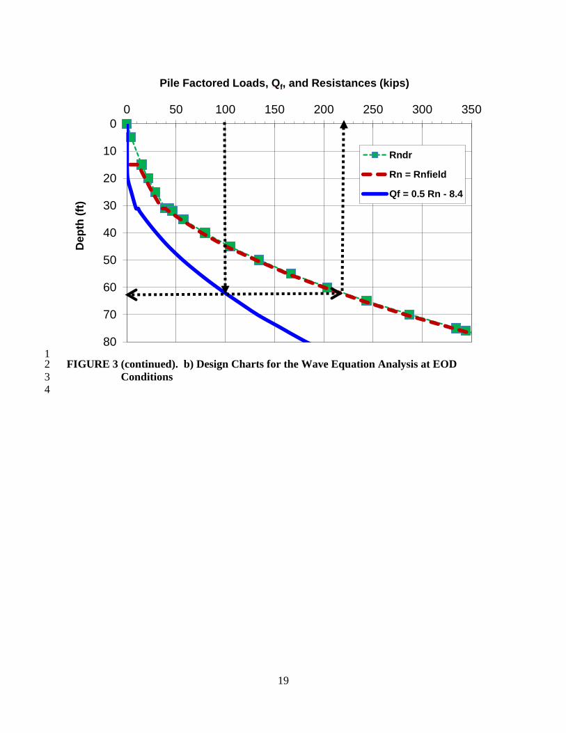
15 DEVELOPMENT AND APPLICATIONS OF DESIGN CHARTS 16 17 The development and applications of the design charts are demonstrated in this section by 18 solving the LRFD design Example. 19 20 β-Method 21 22 The developed design chart in Figure 3a include Rnstat vs. depth curve (Figure 2a) and Qf vs. 23 depth curve obtained using Qf = 0.25Rnstat – 8.4. As demonstrated in this design chart, the 24 required pile length to support Qf of 100 kips is obtained from the design chart as 56 ft using 25 either: 26 • Qf vs. depth curve at Qf= 100 kips 27 • Rnstat vs. depth curve at required Rnstat computed as (100 + 8.4)/0.25 = 433.6 kips. 28 29 Wave Equation Analysis at EOD Conditions. 30 31 The developed design chart in Figure 3b include Rnfield and Rndr vs. depth curves (from Figure 32 2b) and Qf vs. depth curve obtained using Qf = 0.5Rnfield – 8.4. As demonstrated in this design 33 chart: 34 • The pile length to support Qf of 100 kips is estimated as 62 ft, obtained from the Qf vs. depth 35

curve at Qf= 100 kips. 36 • Use the Rndr vs. depth curve and pile length of 62 ft to determine the required Rndr as 220 37

kips. Alternately, the required Rndr can be computed using Eq. 9 as (100 + 8.4)/0.5 + 3.5 = 38 220.3 kips. 39

40 To address uncertainties in the procedure used to estimate the field bearing resistances in the 41 design, the estimated pile length, L, is increased from 62 ft to 67 ft, as previously discussed. 42 43 44 45 46

12

Wave Equation Analysis at BOR Conditions 1 2 The developed design chart in Figure 3c include Rnfield, Rndr, Rnre vs. depth curves (from Figure 3 2b) and Qf vs. depth curve obtained using Qf = 0.5Rnfield – 8.4. As demonstrated in this design 4 chart: 5 • The pile length to support Qf of 100 kips is estimated as 52 ft. 6 • Use the Rnre vs. depth curve and pile length of 52 ft to determine the required Rnre as 220 7

kips. Alternately, the required Rnre may be computed using Eq. 11 as (100 + 8.4)/0.5 + 3.5 = 8 220.3 kips. 9

• Use the Rndr vs. depth curve at a depth of 52 ft to determine the required Rndr as 145 kips. 10 11

To address uncertainties in the procedure used to estimate the field bearing resistance in the 12 design, the estimated pile length, L, is increased from 52 ft to 57 ft. 13 14 Benefits of Setup. Figure 4 suggests that the factored axial compression loads, Qf, that can be 15 supported at various depths are larger with the wave equation analysis at BOR conditions than at 16 EOD conditions due to consideration of setup at BOR conditions. Hence, consideration of setup 17 in the design will lead to either reduced pile length or fewer piles. In the solved example, the 18 consideration of setup at BOR conditions reduced pile length by 10 ft from 67 ft to 57 ft. In 19 conclusion, the consideration of setup in the design would lead to more economical design in 20 most cases. 21 22 Static vs. Field Dynamic Analysis Methods. Figure 4 suggests that the factored axial 23 compression loads, Qf, that can be supported at various depths are larger with the β-Method than 24 the wave equation analysis at EOD, suggesting that the design pile length or number of piles will 25 be smaller with the β-Method. For example, in the solved example, the pile length with the β-26 Method is 56 ft , which is less than length of 67 ft estimated with the wave equation analysis at 27 EOD. This means that consideration of static analysis method to finalize pile length may be more 28 economical than some field analysis methods as also demonstrated by Abu-Hejleh et. al. (2010). 29 Also, benefits of setup can be considered with the static analysis in the design phase without the 30 need for verification of setup in the field. Finally, with selection of static analysis methods to 31 finalize pile length in the design, construction time will be reduced and construction problems 32 could be reduced, for example the problems developed with selection of field analysis methods 33 to finalize pile length as previously discussed. 34 35 Axial Compression Static Load Test 36 37 Since λBOR = 1.0 for the static load test and λstat = 0.61 for the β-method, αBOR for the load test is 38 estimated as 0.61 (0.61/1.0). Then, Rnsta resistances for the β-Method (Figure 2a) were multiplied 39 by αBOR = 0.61 to obtain the Rnfield vs. depth curve for the static load test. Finally, the Qf vs. 40 depth curve for the load test presented in Figure 4 is developed using Qf = 0.75Rnfield – 8.4. As 41 demonstrated in Figure 4, the pile length to support Qf of 100 kips is estimated as 44 ft. This pile 42 length is the smallest pile length among all methods investigated in this paper. The required Rnre 43 that should be verified with the static load test is computed using Eq. 11 as (100 + 8.4)/0.75 + 3.5 44 = 148 kips. 45 46

13

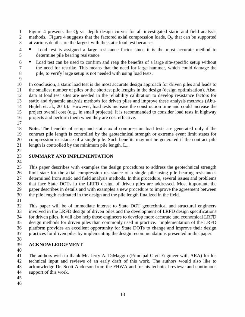
Figure 4 presents the Qf vs. depth design curves for all investigated static and field analysis 1 methods. Figure 4 suggests that the factored axial compression loads, Qf, that can be supported 2 at various depths are the largest with the static load test because: 3 • Load test is assigned a large resistance factor since it is the most accurate method to 4

determine pile bearing resistance 5 • Load test can be used to confirm and reap the benefits of a large site-specific setup without 6

the need for restrike. This means that the need for large hammer, which could damage the 7 pile, to verify large setup is not needed with using load tests. 8

9 In conclusion, a static load test is the most accurate design approach for driven piles and leads to 10 the smallest number of piles or the shortest pile lengths in the design (design optimization). Also, 11 data at load test sites are needed in the reliability calibration to develop resistance factors for 12 static and dynamic analysis methods for driven piles and improve these analysis methods (Abu-13 Hejleh et. al., 2010). However, load tests increase the construction time and could increase the 14 project overall cost (e.g., in small projects). It is recommended to consider load tests in highway 15 projects and perform them when they are cost effective. 16 17 Note. The benefits of setup and static axial compression load tests are generated only if the 18 contract pile length is controlled by the geotechnical strength or extreme event limit states for 19 compression resistance of a single pile. Such benefits may not be generated if the contract pile 20 length is controlled by the minimum pile length, Lm. 21

22 SUMMARY AND IMPLEMENTATION 23 24 This paper describes with examples the design procedures to address the geotechnical strength 25 limit state for the axial compression resistance of a single pile using pile bearing resistances 26 determined from static and field analysis methods. In this procedure, several issues and problems 27 that face State DOTs in the LRFD design of driven piles are addressed. Most important, the 28 paper describes in details and with examples a new procedure to improve the agreement between 29 the pile length estimated in the design and the pile length finalized in the field. 30 31 This paper will be of immediate interest to State DOT geotechnical and structural engineers 32 involved in the LRFD design of driven piles and the development of LRFD design specifications 33 for driven piles. It will also help those engineers to develop more accurate and economical LRFD 34 design methods for driven piles than commonly used in practice. Implementation of the LRFD 35 platform provides an excellent opportunity for State DOTs to change and improve their design 36 practices for driven piles by implementing the design recommendations presented in this paper. 37 38 ACKNOWLEDGEMENT 39 40 The authors wish to thank Mr. Jerry A. DiMaggio (Principal Civil Engineer with ARA) for his 41 technical input and reviews of an early draft of this work. The authors would also like to 42 acknowledge Dr. Scott Anderson from the FHWA and for his technical reviews and continuous 43 support of this work. 44

45 46

14

REFERENCES 1 2 1. AASHTO (American Association of State Highway and Transportation Officials) (2012). 3

“AASHTO LRFD Bridge Design Specifications, 6th Edition,” Washington, D.C. 4 2. Abu-Hejleh, N., DiMaggio, J.A., Kramer, W.M., Anderson, S., and Nichols, S. (2010). 5

“Implementation of LRFD Geotechnical Design for Bridge Foundations.” FHWA-NHI-10-6 039, National Highway Institute, Federal Highway Administration, Washington, D.C. 7

3. Arneson, L.A., Zevenbergen, L.W., Lagasse, P.F., and Clopper, P.E. (2012). “Evaluating 8 Scour at Bridges, 5th Edition.” Hydraulic Engineering Circular No. 18, FHWA-HIF-12-9 003, Federal Highway Administration, Washington, D.C. 10

4. Hannigan, P.J., Goble, G.G., Likens, G.E., and Rausche, F. (2006). “Design and 11 Construction of Drivn Pile Foundations.” FHWA-NHI-05-042, National Highway Institute, 12 Federal Highway Administration, Washington, D.C. 13

5. Paikowsky, S.G., Birgisson, B., McVay, M., Nguyen, T., Kuo, C., Baecher, G., Ayyub, B., 14 Stenersen, K., O’Malley, K., Chernauskas, L., and O’Neill, M. (2004). “Load and 15 Resistance Factor Design (LRFD) for Deep Foundations.” NCHRP Report 507, 16 Transportation Research Board, Washington, D.C. 17

http://www.trb.org/news/blurb_detail.asp?id=4074 18 6. Smith, T., Banas, A., Gummer, M., and Jin, J. (2010). “Recalibration of the GRLWEAP 19

LRFD Resistance Factor for Oregon DOT.” Publication No. OR-RD-98-00, Oregon 20 Department of Transportation, Research Unit, Salem, Oregon. 21

22

15

1 2 3

4

5 6

Figure 1. Some Details of the LRFD Design Example 7 8 9

Loose sand layer: 31 ft Friction angle = 31o Saturated unit weight =110 pcf

12x53 H-pile: fy = 50 ksi As = 15.5 in2 Box area = 1 ft2 Perimeter = 4 ft

Hard clay: Undrained shear strength = 8 ksf Saturated unit weight= 125 pcf, Setup= 50%

Top 15 ft will settle relative to the pile, mobilizing downdrag, γp = 1.4

GWL at ground level

With various static and field analysis methods, determine: Design pile length Required field bearing resistance if needed

Qf (applied factored compression load) = 100 kips

16

1 Figure 2. LRFD Design Example. a) Pile Bearing Resistances the β-Method 2 3

4 5 6

0

10

20

30

40

50

60

70

80

0 100 200 300 400 500 600 700

Dep

th (f

t) Pile Resistances at Various Stages (kips)

Rnre

Rndr

Rn= Rnsta

17

1 Figure 2 (continued). b) Pile Bearing Resistances for Wave Equation Analysis at EOD and 2 BOR Conditions 3 4 5 6 Table 1. Developing the Median: Resistance Bias Factors Between a Field Analysis Method 7

and a Static Analysis Method and Setup Factor. 8 9

10 11 12 13 14 15 16 17 18 19 20 21 22

0

10

20

30

40

50

60

70

80

90

0 100 200 300 400 500D

epth

(ft)

Pile Resistances at Various Stages (kips)

Rndr

Rnre

Rn = Rnfield, BOR Conditions

Rn = Rnfield, EOD Conditions

Rndr αEOD (Field Rndr/

Static Rnre)Rnre

αBOR (Field Rnre/ Static Rnre)

625 410 0.66 512 0.82 25633 504 0.80 610 0.96 21571 308 0.54 381 0.67 24489 409 0.84 470 0.96 15853 475 0.56 590 0.69 24550 426 0.78 533 0.97 25817 412 0.50 515 0.63 25

Median 0.66 0.82 24

Rnre Resistances from Static

Analysis Method (kips)

Resistances from Field Analysis Method (kips)Setup (%)

(Rnre-Rndr)/Rndr

18

1 2

3

4 Figure 3. LRFD Design Example. a) Design Charts for the β-Method 5

19

1 FIGURE 3 (continued). b) Design Charts for the Wave Equation Analysis at EOD 2

Conditions 3 4

0

10

20

30

40

50

60

70

80

0 50 100 150 200 250 300 350

Dep

th (f

t) Pile Factored Loads, Qf, and Resistances (kips)

Rndr

Rn = Rnfield

Qf = 0.5 Rn - 8.4

20

1 FIGURE 3 (continued). c) Design Charts for the Wave Equation Analysis at BOR 2

Conditions 3 4 5 6 7 8

0

10

20

30

40

50

60

70

0 50 100 150 200 250 300 350

Dep

th (f

t) Pile Factored Loads, Qf, and Resistances (kips)

Rnre

Rn = Rnfield

Rndr

Qf = 0.5 Rn - 8.4

21

1 FIGURE 4. Design curves for all investigated Static and Field Analysis Methods 2

0

10

20

30

40

50

60

70

80

0 100 200 300 400D

epth

(ft)

Pile Top Factored Axial Compression Loads, Qf (kips)

Beta Method

Wave Equation Analysis at EOD

Wave Equation Analysis at BOR

Static Load Test`