implementation of the marchenko method
TRANSCRIPT

Implementation of the Marchenko method
Jan Thorbecke1, Evert Slob1, Joeri Brackenhoff1, Joost van der Neut1, and Kees Wapenaar1
ABSTRACT
The Marchenko method makes it possible to computesubsurface-to-surface Green’s functions from reflectionmeasurements at the surface. Applications of the Marchenkomethod have already been discussed in many papers, but itsimplementation aspects have not yet been discussed in de-tail. Solving the Marchenko equation is an inverse problem.The Marchenko method computes a solution of the Marche-nko equation by an (adaptive) iterative scheme or by a directinversion. We have evaluated the iterative implementationbased on a Neumann series, which is considered to be theconventional scheme. At each iteration of this scheme, a con-volution in time and an integration in space are performedbetween a so-called focusing (update) function and the reflec-tion response. In addition, by applying a time window, oneobtains an update, which becomes the input for the next iter-ation. In each iteration, upgoing and downgoing focusingfunctions are updated with these terms. After convergence ofthe scheme, the resulting upgoing and downgoing focusingfunctions are used to compute the upgoing and downgoingGreen’s functions with a virtual-source position in the subsur-face and receivers at the surface. We have evaluated thisalgorithm in detail and developed an implementation that re-produces our examples. The software fits into the SeismicUnix software suite of the Colorado School of Mines.
INTRODUCTION
The Marchenko method relates Green’s function from a virtualsource inside a medium to the reflection response at the surface ofthat medium. The method has been introduced to the geophysicalworld by Broggini and Snieder (2012). In close collaboration with
these authors, their work is extended to 2D and 3D media by Brog-gini et al. (2012) and Wapenaar et al. (2013). Based on the outputsof the Marchenko method, upgoing and downgoing Green’s func-tions can be estimated, for any point in the subsurface to the surfacearray, using the reflection response recorded at the surface. TheGreen’s function is the earth impulse response and is fundamentalin many processing schemes.The application of the results of the Marchenko method is there-
fore manifold: It has been used for imaging the subsurface withoutthe disturbing effect of internal multiples (Behura et al., 2014; Slobet al., 2014; Wapenaar et al., 2014b; da Costa Filho et al., 2015; vander Neut et al., 2015c; Vasconcelos et al., 2015; Meles et al., 2016;Ravasi et al., 2016), internal multiple elimination in the data domain(Meles et al., 2015; van der Neut and Wapenaar 2016; da CostaFilho et al., 2017), and retrieving the homogeneous Green’s func-tion between any two points inside a medium from the reflectionresponse (Wapenaar et al., 2017).In the first geophysical Marchenko papers, the computation of
the Green’s function is based on iteratively updating acoustic pres-sure fields (Wapenaar et al., 2013). This pressure-based algorithmrequires two separate iterative updates to calculate the upgoing ordowngoing Green’s functions at a virtual source position. Slob et al.(2014) combine these separate iterative schemes into one. In thiscombined scheme, upgoing and downgoing focusing functionsare updated in each iteration. Wapenaar and Slob (2014) and daCosta Filho et al. (2014) extend the method to elastic media, Singhet al. (2015) include the free-surface multiples, and Slob (2016)adapts the method to dissipative acoustic media. Apart from itera-tive schemes, the Marchenko method can also be implemented as anadaptive subtraction (Staring et al., 2016) or a least-squares inver-sion (van der Neut et al., 2015b; Slob and Wapenaar, 2017).In this paper, we describe in detail the implementational aspects
of the 2D iterative acoustic-Marchenko method based on focusingfunctions. Although the algorithm is straightforward to implement,the treatment of amplitudes and the initialization steps of the firstiterations require special attention. The input of the method is a
Peer-reviewed code related to this article can be found at http://software.seg.org/2017/0007.Manuscript received by the Editor 17 February 2017; revised manuscript received 8 June 2017; published ahead of production 21 July 2017; published online
06 September 2017.1Delft University of Technology, Department of Geoscience and Engineering, GA Delft, Delft, The Netherlands. E-mail: [email protected]; e.c.slob@
tudelft.nl; [email protected]; [email protected]; [email protected].© 2017 Society of Exploration Geophysicists. All rights reserved.
WB29
GEOPHYSICS, VOL. 82, NO. 6 (NOVEMBER-DECEMBER 2017); P. WB29–WB45, 12 FIGS., 1 TABLE.10.1190/GEO2017-0108.1
Dow
nloa
ded
09/1
0/17
to 1
45.9
4.65
.141
. Red
istr
ibut
ion
subj
ect t
o SE
G li
cens
e or
cop
yrig
ht; s
ee T
erm
s of
Use
at h
ttp://
libra
ry.s
eg.o
rg/
reflection response without free-surface multiples, and it is decon-volved by its source wavelet. The output of a surface-related multi-ple elimination (SRME) scheme can (in principle) provide thisreflection response. A (smooth) background model is needed to cal-culate an initial focusing function to start the algorithm. The“Numerical examples” section demonstrates the use of the algo-rithm and provides a user’s first steps with the Marchenkotechnique.The software bundled with this paper contains all source code and
scripts to reproduce the examples presents herein. The code can alsobe found at its GitHub repository (Thorbecke, 2017). The GitHubrepository contains the most up-to-date stable version with bug fixesand the latest developments. In Appendix A, the input parameters ofthe programs are explained. To reproduce the figures in this manu-script and to carry out a few post- and preprocessing steps, SeismicUnix (SU) (Cohen and Stockwell, 2016) is required.
MARCHENKO METHOD
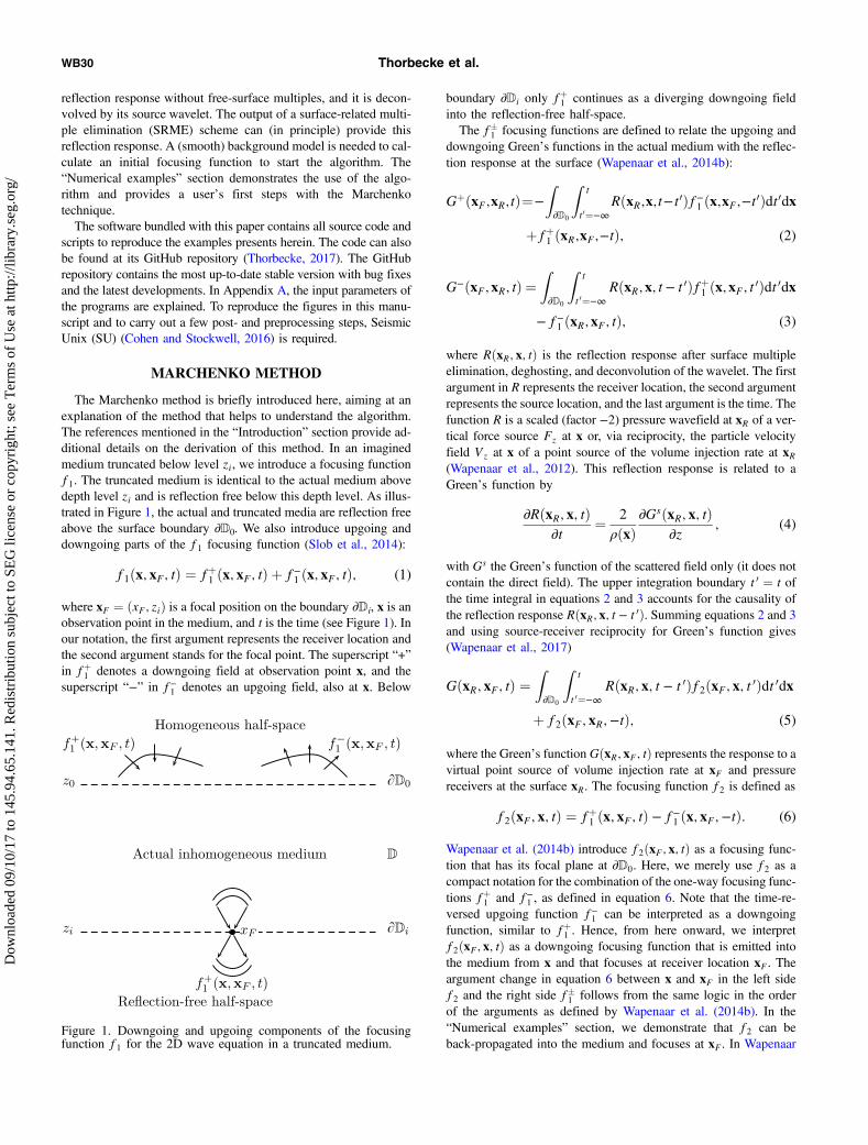
The Marchenko method is briefly introduced here, aiming at anexplanation of the method that helps to understand the algorithm.The references mentioned in the “Introduction” section provide ad-ditional details on the derivation of this method. In an imaginedmedium truncated below level zi, we introduce a focusing functionf1. The truncated medium is identical to the actual medium abovedepth level zi and is reflection free below this depth level. As illus-trated in Figure 1, the actual and truncated media are reflection freeabove the surface boundary ∂D0. We also introduce upgoing anddowngoing parts of the f1 focusing function (Slob et al., 2014):
f1ðx; xF; tÞ ¼ fþ1 ðx; xF; tÞ þ f−1 ðx; xF; tÞ; (1)
where xF ¼ ðxF; ziÞ is a focal position on the boundary ∂Di, x is anobservation point in the medium, and t is the time (see Figure 1). Inour notation, the first argument represents the receiver location andthe second argument stands for the focal point. The superscript “+”in fþ1 denotes a downgoing field at observation point x, and thesuperscript “−” in f−1 denotes an upgoing field, also at x. Below
boundary ∂Di only fþ1 continues as a diverging downgoing fieldinto the reflection-free half-space.The f�1 focusing functions are defined to relate the upgoing and
downgoing Green’s functions in the actual medium with the reflec-tion response at the surface (Wapenaar et al., 2014b):
GþðxF;xR;tÞ¼−Z∂D0
Zt
t0¼−∞RðxR;x;t−t0Þf−1 ðx;xF;−t0Þdt0dx
þfþ1 ðxR;xF;−tÞ; (2)
G−ðxF;xR; tÞ ¼Z∂D0
Zt
t 0¼−∞RðxR;x; t− t 0Þfþ1 ðx;xF; t 0Þdt 0dx
− f−1 ðxR;xF; tÞ; (3)
where RðxR; x; tÞ is the reflection response after surface multipleelimination, deghosting, and deconvolution of the wavelet. The firstargument in R represents the receiver location, the second argumentrepresents the source location, and the last argument is the time. Thefunction R is a scaled (factor −2) pressure wavefield at xR of a ver-tical force source Fz at x or, via reciprocity, the particle velocityfield Vz at x of a point source of the volume injection rate at xR(Wapenaar et al., 2012). This reflection response is related to aGreen’s function by
∂RðxR; x; tÞ∂t
¼ 2
ρðxÞ∂GsðxR; x; tÞ
∂z; (4)
with Gs the Green’s function of the scattered field only (it does notcontain the direct field). The upper integration boundary t 0 ¼ t ofthe time integral in equations 2 and 3 accounts for the causality ofthe reflection response RðxR; x; t − t 0Þ. Summing equations 2 and 3and using source-receiver reciprocity for Green’s function gives(Wapenaar et al., 2017)
GðxR; xF; tÞ ¼Z∂D0
Zt
t 0¼−∞RðxR; x; t − t 0Þf2ðxF; x; t 0Þdt 0dx
þ f2ðxF; xR;−tÞ; (5)
where the Green’s function GðxR; xF; tÞ represents the response to avirtual point source of volume injection rate at xF and pressurereceivers at the surface xR. The focusing function f2 is defined as
f2ðxF; x; tÞ ¼ fþ1 ðx; xF; tÞ − f−1 ðx; xF;−tÞ: (6)
Wapenaar et al. (2014b) introduce f2ðxF; x; tÞ as a focusing func-tion that has its focal plane at ∂D0. Here, we merely use f2 as acompact notation for the combination of the one-way focusing func-tions fþ1 and f−1 , as defined in equation 6. Note that the time-re-versed upgoing function f−1 can be interpreted as a downgoingfunction, similar to fþ1 . Hence, from here onward, we interpretf2ðxF; x; tÞ as a downgoing focusing function that is emitted intothe medium from x and that focuses at receiver location xF. Theargument change in equation 6 between x and xF in the left sidef2 and the right side f�1 follows from the same logic in the orderof the arguments as defined by Wapenaar et al. (2014b). In the“Numerical examples” section, we demonstrate that f2 can beback-propagated into the medium and focuses at xF. In Wapenaar
Figure 1. Downgoing and upgoing components of the focusingfunction f1 for the 2D wave equation in a truncated medium.
WB30 Thorbecke et al.
Dow
nloa
ded
09/1
0/17
to 1
45.9
4.65
.141
. Red
istr
ibut
ion
subj
ect t
o SE
G li
cens
e or
cop
yrig
ht; s
ee T
erm
s of
Use
at h
ttp://
libra
ry.s
eg.o
rg/

et al. (2013), a (reciprocal) relation between f2ðxF; x; tÞ and adowngoing wavefield pþðx; xF; tÞ is given. Together with pþ thereis also a p− defined, the upgoing reflection response at x from thefocal point at xF. The sum of pþ and p− gives also the Green’sfunction of equation 5. The p� functions are just a different notationof the Marchenko method and can be used to compute the Green’sfunctions in a convenient way. These p� functions are thereforeused in the implementation to compute the Green’s function. Froman educational point of view, the Marchenko method is more easilyunderstood using the focusing functions only, and we will continuealong that way.The above equations, on which the following implementation is
based on, use pressure-normalized fields. Other papers derive sim-ilar equations based on flux-normalized fields (Wapenaar et al.,2014a; Singh et al., 2015; van der Neut et al., 2015b). The relation-ship between pressure- and flux-normalized representations is ex-plained by Wapenaar et al. (2014a).TheMarchenko algorithm estimates focusing functions fþ1 ðx;xF;tÞ
and f−1 ðx; xF; tÞ. However, equations 2 and 3 are by themselves in-sufficient to determine f1; there are four unknowns, but only twoequations. We can eliminate two unknowns by exploiting the fact thatthe focusing functions and Green’s functions have different causalityproperties in the time-space domain. Based on the principle of cau-sality, we know that no energy arrives before the first arrivaltdðxR; xFÞ; hence, the Green’s function GðxR; xF; t < tdðxR; xFÞÞis zero. This also holds for the upgoing and downgoing Green’s func-tions and leads to
0 ¼ −Z∂D0
Zt
t 0¼−∞RðxR; x; t − t 0Þf−1 ðx; xF;−t 0Þdt 0dx
þ fþ1 ðxR; xF;−tÞ; (7)
0 ¼Z∂D0
Zt
t 0¼−∞RðxR; x; t − t 0Þfþ1 ðx; xF; t 0Þdt 0dx
− f−1 ðxR; xF; tÞ; (8)
where t < tdðxR; xFÞ in both equations above.The combination of equations 7 and 8 is known as the Marchenko
equation. These equations form the basis of the iterative scheme,which estimates focusing functions fþ1 and f−1 . In Wapenaar et al.(2014a), the relation
fþ1 ðx; xF; tÞ ¼ T invðxF; x; tÞ (9)
is used to derive an initial estimate for fþ1 that can start the inversionscheme. In equation 9, T invðxF; x; tÞ is the inverse of the transmis-sion response of the truncated medium, which is equal to the actualmedium between ∂D0 and ∂Di, for a source at x (at ∂D0) and areceiver at ∂Di. It is assumed that this inverse transmission responseT inv can be composed as a direct wave followed by scattering coda(van der Neut et al., 2015b):
fþ1 ðx; xF; tÞ ¼ T invd ðxF; x; tÞ þMþðx; xF; tÞ; (10)
where Mþ is the unknown scattering coda and T invd is the direct
arrival of the inverse transmission response. In equation 10, the in-verse of the direct arrival of the transmission response is needed. Forsimplicity, we take the time reversal of the direct arrival of Green’sfunction; Gdðx; xF;−tÞ:
fþ1 ðx; xF; tÞ ≈ Gdðx; xF;−tÞ þMþðx; xF; tÞ: (11)
We thereby introduce an overall scaling error and an offset-depen-dent amplitude error, proportional to transmission losses, in the finalresult. The function Gdðx; xF;−tÞ is the time-reversed direct arrivalpart of the transmission response to subsurface focal point xF andcan, for example, be computed from a smooth macromodel. Asmentioned before, the arrival time of Gdðx; xF; tÞ is td; hence,Gdðx; xF; tÞ is zero before t < td. The multiple scattering codaMþðx; xF; tÞ follows after the first arrival of fþ1 , and it is zerofor t ≤ −td. It can also be shown that it is also zero for t ≥ þtd (Slobet al., 2014).Equations 7 and 8 are only valid for t < td. Therefore, we define a
time-window function:
θðxR; xF; tÞ ¼8<:
1 t < tεd12
t ¼ tεd0 t > tεd
; (12)
where time tεd is the time of the direct arrival from the focal point xFto xR (td), minus a small positive constant ε to exclude the waveletin the direct arrival Gd. For example, a time window that sets alltimes t < −tεd to zero and applied to equation 11 mutes Gdð−tÞ,but it leaves all events of Mþ in. In the following, we will usethe shorthand notation θt for θðxR; xF; tÞ. In the included Marchen-ko program, there is an input parameter (called smooth; see Ap-pendix A for all input parameters) that defines a temporal taperingin this mute window to suppress high-frequency artifacts.It is further assumed that it is possible to get an estimate of this
direct arrival Gd of the transmission response. Given the reflectionresponse RðxR; x; tÞ and this direct arrival Gdðx; xF; tÞ from the fo-cal point, the Marchenko algorithm solves for the scattering codaMþðx; xF; tÞ to estimate fþ1 ðx; xF; tÞ and f−1 ðx; xF; tÞ.The iterative solution of the Marchenko equations can now be
developed. The iterative scheme is started with the following ini-tialization of Mþ:
Mþ0 ðxR; xF; tÞ ¼ 0: (13)
The subscript in Mþ0 defines the iteration number. By substituting
equation 11, using 13 as an initialization, into equation 8 one arrivesat the initialization of f−1 :
f−1;0ðxR; xF; tÞ
¼ θt
Z∂D0
Zt
t 0¼−∞RðxR; x; t − t 0ÞGdðx; xF;−t 0Þdt 0dx:
(14)
Equation 14 includes the previously defined time-window functionθt. Equations 7 and 11 are expressions for fþ1 . By combining theseequations, the only part remaining in equation 11 is Mþ. The iter-ative update of Mþ for step k ≥ 1 is given by
Mþk ðxR; xF;−tÞ
¼ θt
Z∂D0
Zt
t 0¼−∞RðxR; x; t − t 0Þf−1;k−1ðx; xF;−t 0Þdt 0dx:
(15)
Marchenko method WB31
Dow
nloa
ded
09/1
0/17
to 1
45.9
4.65
.141
. Red
istr
ibut
ion
subj
ect t
o SE
G li
cens
e or
cop
yrig
ht; s
ee T
erm
s of
Use
at h
ttp://
libra
ry.s
eg.o
rg/

Following the assumption in equation 11, that it is possible to writefþ1;k as a direct field plus scattering coda, the update at step k of f
þ1;k
is given by
fþ1;kðxR; xF; tÞ ¼ GdðxR; xF;−tÞ þMþk ðxR; xF; tÞ: (16)
Using equation 8 and the expression of fþ1 in equation 16, the up-date of f−1 at step k is given by
f−1;kðxR; xF; tÞ ¼ f−1;0ðxR; xF; tÞ
þ θt
Z∂D0
Zt
t 0¼−∞RðxR; x; t − t 0ÞMþ
k ðx; xF; t 0Þdt 0dx: (17)
This completes the definition of the iterative Marchenko scheme.In the next section, the first few iterations are discussed in detail andillustrated with simple numerical examples.
MARCHENKO ALGORITHM
To compute f1 focusing functions with the Marchenko method,two ingredients are needed:
• Reflection data without free-surface multiples, ghosts anddeconvolved for the wavelet: RðxR; x; tÞ with source x andreceiver xR on the same surface ∂D0, and small enough sam-pling for xR and x to avoid spatial aliasing.
• An estimate of the direct arrival between the receiver posi-tions at the surface (xR), and the focal point at xF:GdðxR; xF; tÞ, and derived from it the direct arrival timetdðxR; xF; tÞ. Note that td can also be computed by anothermethod, for example, an eikonal solver.
Given these two components, the iterative method can be initial-ized and the iterations of the Marchenko method can start.
The first few iterations
The initialization of the method is given in equations 13 and 14.The time-windowed expression for f−1;0ðxR; xF; tÞ in equation 14 isrenamed to
− N0ðxR; xF;−tÞ
¼ θt
Z∂D0
Zt 0RðxR; x; t − t 0ÞGdðx; xF;−t 0Þdt 0dx: (18)
At each iteration, the spatial integration and temporal convolutionwith R plays an important role because it is used to define new fo-cusing updates given by terms Ni (see also appendix B of Wapenaaret al., 2014b). These Ni terms are used to update the estimates of thefocusing functions fþ1 and f−1 . Although theNi terms are not strictlyneeded to describe the method, they are introduced here to remainas close as possible to the actual implementation.For computational efficiency, the temporal convolution of R is
implemented in the Fourier domain. The spatial integration is car-ried out by summing the resulting traces of the time convolutionover a common-receiver gather. The introduced time-window setsevents for t > tεd to zero, in accordance with equation 18. Applyingthe mute window is therefore a crucial and mandatory step in theMarchenko method; without it, the method would be incorrect.
Given these initializations, the first step in the algorithm, basedon equations 15–17, can be computed. This first step, k ¼ 1, in-volves two integration-convolutions with R to update fþ1 and f−1 :
Mþ1 ðxR;xF;−tÞ¼θt
Z∂D0
Zt 0RðxR;x;t− t 0Þf−1;0ðx;xF;−t 0Þdt 0dx
¼−θtZ∂D0
Zt 0RðxR;x;t− t 0ÞN0ðx;xF;t 0Þdt 0dx
¼N1ðxR;xF;−tÞ; (19)
fþ1;1ðxR; xF; tÞ ¼ GdðxR; xF;−tÞ þMþ1 ðxR; xF; tÞ
¼ GdðxR; xF;−tÞ þ N1ðxF; xR; tÞ; (20)
f−1;1ðxR;xF; tÞ ¼ f−1;0ðxR;xF; tÞ
þ θt
Z∂D0
Zt 0RðxR;x; t− t 0ÞMþ
1 ðx;xF; t 0Þdt 0dx
¼−N0ðxR;xF;−tÞ
þ θt
Z∂D0
Zt 0RðxR;x; t− t 0ÞN1ðx;xF; t 0Þdt 0dx;
¼−N0ðxR;xF;−tÞ−N2ðxR;xF;−tÞ; (21)
f2;1ðxF; xR; tÞ ¼ GdðxR; xF;−tÞ þ N0ðxR; xF; tÞþ N1ðxR; xF; tÞ þ N2ðxR; xF; tÞ: (22)
The first integration-convolution with R in equation 19 is used toupdate fþ1 as shown in equation 20. The second integration-convo-lution in equation 21 updates f−1 . The update of f2, introduced inequation 6, includes the results of all integration-convolutionswith R.The next step for k ¼ 2 results in the following updates:
Mþ2 ðxR;xF;−tÞ¼θt
Z∂D0
Zt 0RðxR;x;t− t 0Þf−1;1ðx;xF;−t 0Þdt 0dx
¼−θtZ∂D0
Zt 0RðxR;x;t− t 0ÞfN0ðx;xF;tÞ
þN2ðx;xF;tÞgdt 0dx¼N1ðxR;xF;−tÞþN3ðxR;xF;−tÞ; (23)
fþ1;2ðxR; xF; tÞ ¼ GdðxR; xF;−tÞ þMþ2 ðxR; xF; tÞ
¼ GdðxR; xF;−tÞ þ N1ðxR; xF; tÞþ N3ðxR; xF; tÞ; (24)
WB32 Thorbecke et al.
Dow
nloa
ded
09/1
0/17
to 1
45.9
4.65
.141
. Red
istr
ibut
ion
subj
ect t
o SE
G li
cens
e or
cop
yrig
ht; s
ee T
erm
s of
Use
at h
ttp://
libra
ry.s
eg.o
rg/

f−1;2ðxR;xF;tÞ¼f−1;0ðxR;xF;tÞ
þθt
Z∂D0
Zt 0RðxR;x;t− t 0ÞMþ
2 ðx;xF;t 0Þdt 0dx
¼−N0ðxR;xF;−tÞþθt
Z∂D0
Zt 0RðxR;x;t− t 0Þ
×fN1ðx;xF;tÞþN3ðx;xF;tÞgdt 0dx¼−N0ðxR;xF;−tÞ−N2ðxR;xF;−tÞ−N4ðxR;xF;−tÞ; (25)
f2;2ðxF; xR; tÞ ¼ GdðxR; xF;−tÞ þ N0ðxR; xF; tÞþ N1ðxR; xF; tÞ þ N2ðxR; xF; tÞþ N3ðxR; xF; tÞ þ N4ðxR; xF; tÞ: (26)
From these updates, it becomes clear that in updating fþ1 in equa-tion 24 Gd and the odd terms of Ni are used and in updating f−1 inequation 25 the even terms of Ni are used. The f2 function in equa-tion 26 is built up from Gd and even and odd Ni terms.In the implementation, the Ni terms are computed by
N−1ðxR; xF;−tÞ ¼ Gdðx; xF;−t 0Þ; (27)
NiðxR;xF;−tÞ¼−θtZ∂D0
Zt 0RðxR;x;t− t 0ÞNi−1ðx;xF;t 0Þdt 0dx;
(28)
and are used to update the focusing functions fþ1 ; f−1 , and f2. This
makes the algorithm simple and efficient. In summary, the relationsfor Mþ
m;Ni and the updates for the focusing functions for m iter-ations with m ≥ 1 are
MþmðxR; xF; tÞ ¼
Xm−1
l¼0
N2lþ1ðxR; xF; tÞ; (29)
fþ1;mðxR; xF; tÞ ¼ GdðxR; xF;−tÞ þXm−1
l¼0
N2lþ1ðxR; xF; tÞ;
(30)
f−1;mðxR; xF; tÞ ¼ −Xml¼0
N2lðxR; xF;−tÞ; (31)
f2;mðxF; xR; tÞ ¼ GdðxR; xF;−tÞ þX2ml¼0
NlðxR; xF; tÞ: (32)
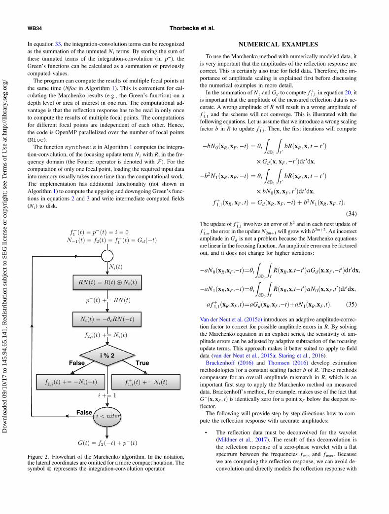
In the provided program, each computation of a focusing updateterm Ni is called one iteration. The implementation is shown in Al-gorithm 1, and a flowchart is shown in Figure 2.The initializations of f−1 , f
þ1 , f2, and Ni are done just before the
iteration starts. The even and odd iterations for Ni update f−1 and
fþ1 , respectively. The Green’s function is computed by inserting theestimate of f2 given by equation 32 into equation 5:
GðxF;xR;tÞ¼f2ðxF;xR;−tÞ
þZ∂D0
Zt
t 0¼−∞RðxR;x;t− t 0ÞGdðx;xF;−tÞdt 0dx
þX2ml¼0
Z∂D0
Zt
t 0¼−∞RðxR;x;t− t 0ÞNlðx;xF;t 0Þdt 0dx:
(33)
Algorithm 1. The Marchenko algorithm as implemented inthe provided source code.
Marchenko method WB33
Dow
nloa
ded
09/1
0/17
to 1
45.9
4.65
.141
. Red
istr
ibut
ion
subj
ect t
o SE
G li
cens
e or
cop
yrig
ht; s
ee T
erm
s of
Use
at h
ttp://
libra
ry.s
eg.o
rg/
In equation 33, the integration-convolution terms can be recognizedas the summation of the unmuted Ni terms. By storing the sum ofthese unmuted terms of the integration-convolution (in p−), theGreen’s functions can be calculated as a summation of previouslycomputed values.The program can compute the results of multiple focal points at
the same time (Nfoc in Algorithm 1). This is convenient for cal-culating the Marchenko results (e.g., the Green’s function) on adepth level or area of interest in one run. The computational ad-vantage is that the reflection response has to be read in only onceto compute the results of multiple focal points. The computationsfor different focal points are independent of each other. Hence,the code is OpenMP parallelized over the number of focal points(Nfoc).The function synthesis in Algorithm 1 computes the integra-
tion-convolution, of the focusing update term Ni with R, in the fre-quency domain (the Fourier operator is denoted with F ). For thecomputation of only one focal point, loading the required input datainto memory usually takes more time than the computational work.The implementation has additional functionality (not shown inAlgorithm 1) to compute the upgoing and downgoing Green’s func-tions in equations 2 and 3 and write intermediate computed fields(Ni) to disk.
NUMERICAL EXAMPLES
To use the Marchenko method with numerically modeled data, itis very important that the amplitudes of the reflection response arecorrect. This is certainly also true for field data. Therefore, the im-portance of amplitude scaling is explained first before discussingthe numerical examples in more detail.In the summation of N1 and Gd to compute fþ1;1 in equation 20, it
is important that the amplitude of the measured reflection data is ac-curate. A wrong amplitude of R will result in a wrong amplitude offþ1;1 and the scheme will not converge. This is illustrated with thefollowing equations. Let us assume that we introduce a wrong scalingfactor b in R to update fþ1;i. Then, the first iterations will compute
−bN0ðxR; xF;−tÞ ¼ θt
Z∂D0
Zt 0bRðxR; x; t − t 0Þ
× Gdðx; xF;−t 0Þdt 0dx;
−b2N1ðxR; xF;−tÞ ¼ θt
Z∂D0
Zt 0bRðxR; x; t − t 0Þ
× bN0ðx; xF; t 0Þdt 0dx;fþ1;1ðxR; xF; tÞ ¼ GdðxR; xF;−tÞ þ b2N1ðxR; xF; tÞ:
(34)
The update of fþ1;1 involves an error of b2 and in each next update of
fþ1;m the error in the updateN2mþ1 will growwith b2mþ2. An incorrectamplitude in Gd is not a problem because the Marchenko equationsare linear in the focusing function. An amplitude error can be factoredout, and it does not change for higher iterations:
−aN0ðxR;xF;−tÞ¼θt
Z∂D0
Zt0RðxR;x;t−t0ÞaGdðx;xF;−t0Þdt0dx;
−aN1ðxR;xF;−tÞ¼θt
Z∂D0
Zt0RðxR;x;t−t0ÞaN0ðx;xF;t0Þdt0dx;
afþ1;1ðxR;xF;tÞ¼aGdðxR;xF;−tÞþaN1ðxR;xF;tÞ: (35)
Van der Neut et al. (2015c) introduces an adaptive amplitude-correc-tion factor to correct for possible amplitude errors in R. By solvingthe Marchenko equation in an explicit series, the sensitivity of am-plitude errors can be adjusted by adaptive subtraction of the focusingupdate terms. This approach makes it better suited to apply to fielddata (van der Neut et al., 2015a; Staring et al., 2016).Brackenhoff (2016) and Thomsen (2016) develop estimation
methodologies for a constant scaling factor b of R. These methodscompensate for an overall amplitude mismatch in R, which is animportant first step to apply the Marchenko method on measureddata. Brackenhoff’s method, for example, makes use of the fact thatG−ðx; xF; tÞ is identically zero for a point xF below the deepest re-flector.The following will provide step-by-step directions how to com-
pute the reflection response with accurate amplitudes:
• The reflection data must be deconvolved for the wavelet(Mildner et al., 2017). The result of this deconvolution isthe reflection response of a zero-phase wavelet with a flatspectrum between the frequencies fmin and fmax. Becausewe are computing the reflection response, we can avoid de-convolution and directly models the reflection response with
Figure 2. Flowchart of the Marchenko algorithm. In the notation,the lateral coordinates are omitted for a more compact notation. Thesymbol ⊛ represents the integration-convolution operator.
WB34 Thorbecke et al.
Dow
nloa
ded
09/1
0/17
to 1
45.9
4.65
.141
. Red
istr
ibut
ion
subj
ect t
o SE
G li
cens
e or
cop
yrig
ht; s
ee T
erm
s of
Use
at h
ttp://
libra
ry.s
eg.o
rg/

a source signature that has a flat frequency spectrum of am-plitude 1.0:
sðtÞ ¼Z
fmax
fmin
1.0 expð−j2πftÞdf: (36)
The implemented flat wavelet spectrum has smooth transitions(a cosine taper) to the minimum, and from the maximum, frequencyto avoid a very long wavelet in the time domain. The provided pro-gram makewave can generate these waveforms and the providedscripts give the makewave parameters used to calculate the sourcewavelet. Note: In the discrete implementation of the computation ofthe source wavelet in the frequency domain, one must not forget tomultiply with the frequency interval Δf, when going from fre-quency to time with the Fourier transform. The source wavelet usedin the examples is shown in Figure 3. A shift of 0.3 s (the parametersetting t0=0.3 in makewave) is added to the source wavelet tomake it causal and suitable to use in the finite-difference program.In the finite-difference modeling of the reflection response, the re-cording of the data is postponed with 0.3 s (parameter settingrec_delay = 0.3 in fdelmodc) to set the peak of the waveletback at the correct time.
• In the finite-difference program for modeling RðxR; x; tÞ, anFz source of vertical force is chosen (see the manual of thefinite-difference modeling program fdelmodc for an ex-planation about the options). The receivers are placed atthe same surface as the source and measure the pres-sure field.
• The amplitude scaling factor, in the finite-difference schemefor an Fz source with time signature sðtÞ, is defined in theupdate of particle velocity Vz as
Vzðx; z; tþ ΔtÞ ¼ Vzðx; z; tÞ −ΔPðx; z; tÞ
ρΔzþ Δt
ρΔx2sðtÞ:
(37)
The discrete intervals Δt;Δx ¼ Δz are the steps in the finite-differ-ence program, and ρ is the local density at the injection grid point ofthe source. The term ΔP∕Δz is a fourth-order finite-difference im-plementation of the first derivative to z of pressure field P
• To compute R, from Green’s functions calculated by the fi-nite-difference program, only a factor of −2 is needed (equa-tion 10 in Wapenaar et al., 2012). This factor −2 is includedin the marchenko program when it reads in the reflectionresponse R.
• The time convolution of R is implemented by a forward Fou-rier transformation from the time to the frequency domain,multiplication in the frequency domain, and back-transfor-mation to the time domain. In the numerical implementation,the multiplication with Δt, for the convolution in time andwith Δx for the integration over x, must be included as well.Together with the standard scaling factor of 1∕N for discreteFourier transformations when going from the time to the fre-quency domain and back to the time domain, with N thenumber of time samples, the scale factor to compute the time
convolution and space integration in the frequency domainbecomes
ΔxΔtN
: (38)
Building up the Green’s function
The Marchenko algorithm is illustrated with a 2D horizontallylayered model as shown in Figure 4. The numerical modeling iscarried out with a finite-difference modeling program (Thorbeckeand Draganov, 2011) that is also included in the software package.The input source signature used to model the reflection responseRðxR; x; tÞ is approximately a sinc function with a flat spectrumof amplitude 1, as shown in Figure 3.The full reflection matrix RðxR; x; tÞ, for a fixed-spread geometry,
can be constructed from one forward-modeled shot (Figure 4c) be-cause the model contains no lateral variations. The constructedfixed-spread geometry ranges from −2250 to 2250 m with a 5 mdistance between the source and receiver positions. The 5 m dis-tance is chosen to avoid spatial aliasing. We use a laterally invariantmedium because the time to compute the reflection response R in alaterally variant medium is too large to be practical for the desiredreproducibility of the examples in this paper. However, the Marche-nko method does not make any assumption about the medium andcan handle lateral variations as well. Moreover, the demo directory
0 0.2 0.3 0.5 0.6 0.8 0.9Time (s)
0
a)
b)
100
Am
plitu
de
0 10 20 30 40 50 60 70 80 90 100 110 120
Frequency (1/s)
0.5
1.0
Am
plitu
de
Figure 3. Source wavelet with a flat frequency spectrum betweenfminð¼ 5 HzÞ and fmaxð¼ 80 HzÞ used to model the reflection re-sponse.
Marchenko method WB35
Dow
nloa
ded
09/1
0/17
to 1
45.9
4.65
.141
. Red
istr
ibut
ion
subj
ect t
o SE
G li
cens
e or
cop
yrig
ht; s
ee T
erm
s of
Use
at h
ttp://
libra
ry.s
eg.o
rg/

of the Marchenko program contains also an example with lateralvariations in the model (marchenko/demo/twoD).The transmission response, recorded at the surface for a source at
a 900 m depth, is shown in Figure 4d. It has been modeled with azero-phase Ricker source wavelet sðtÞ that has its peak at 25 Hz. It isimportant that the chosen source wavelet to model Gd be zerophase; otherwise, the time reversals applied in the algorithm wouldnot work properly and the Marchenko scheme would not converge.It is also preferable to choose a source wavelet that decreases rap-idly in time. This is to minimize the occurrence of overlap betweenthe direct arrival and the first reflections as is assumed in equa-tion 11. In case of an overlap, the defined window function (θt inequation 12) cuts through the overlapping events, and the first re-flection is not retrieved correctly.The initialization step used to compute f−1;0 (equation 18) is illus-
trated in Figure 5. Each shot record in RðxR; x; tÞ is convolvedwith GdðxR; xF;−tÞ, where GdðxR; xF;−tÞ shown in Figure 5only contains the time reversal of the full transmission responseas shown in Figure 4d. By making use of shift invarianceRðxR; x; tÞ ¼ RðxR − x; 0; tÞ, the time-convolution result is inte-grated (summed over all receiver positions xR) and results in onetrace at the x position in the N0 panel.In −N0ðx; xF;−tÞ, the dotted lines indicate the cutoff boundaries
of the implemented time window θðx; xF; tÞ. To suppress wrap-around events (from positive times wrapping to negative times),the time window θðx; xF; tÞ, as introduced in equation 12, is sym-metrized. Hence, from here onward θðx; xF; tÞ is zero for t > tεd andt < −tεd, and unity for times inside −tεd < t < tεd. For deep focalpoints, one can also extend the time axis by padding zeros at
the end of the array and in that way avoid the influence ofwrap-around events in the time domain. In Appendix A, the treat-ment of time wrap-around is explained in more detail.The events before the top dotted line and the events after the
bottom dotted line are muted. The two remaining events originatefrom the two reflectors above the chosen focal point at a 900 mdepth. A detailed explanation of the different events in the focus-ing functions is given by van der Neut et al. (2015b). Staring et al.(2016) give a similar explanation in case free-surface multiples areincluded in the Marchenko method. This initialization of f−1 is theinput of the next step to compute a first estimate of fþ1 , given inequations 19 and 20.The computation of fþ1;1 involves the same time convolution and
spatial integration operation, and it is illustrated in Figure 6. Theresult of the integration and convolution; −N1ðx; xF;−tÞ is, accord-ing to equation 20, time reversed, multiplied by −1 and added toGdðx; xF;−tÞ to get the first estimate fþ1;1. Note, that the lower(causal) part of the time window θðx; xF; tÞ mutes also the eventat direct arrival time. This event at the direct arrival time td willend up in the update of the Green’s function and will adjust theamplitude of the direct arrival in the Green’s function (van der Neutet al., 2015b). This update of the direct arrival in the Green’s func-tion is explained in more detail below.Figure 7 shows the results of the first four iterations of the
Marchenko method. The first column represents the results of eachconvolution and integration of the focusing update term Ni with R.From these figure parts (all with the same clipping factor) one canobserve that the amplitude of Ni becomes smaller with each nextiteration.
0
200
400
600
800
1000
1200
1400
Dep
th (
m)
–2000 –1000 0 1000 2000Lateral distance (m)
–2000 –1000 0 1000 2000Lateral distance (m)
1800
2000
2200
2400
0
a)
b)
c) d)
200
400
600
800
1000
1200
1400
Dep
th (
m)
1000
2000
3000
4000
0
0.4
0.8
1.2
1.6
2.0
Tim
e (s
)
0
0.4
0.8
1.2
1.6
2.0
Tim
e (s
)
–2000 –1000 0 1000 2000Lateral distance (m)
–2000 –1000 0 1000 2000Lateral distance (m)
Figure 4. Four-layer model with (a) velocity and (b) density contrasts. (c) A shot record, with source position xðx ¼ 0; z ¼ 0Þ and receivers atxRðx ¼ xr; z ¼ 0Þ, and (d) the transmission response from a source at xFðx ¼ 0; z ¼ 900Þ. Note that the source wavelet used to compute R(c) is given in Figure 3 and T (d) is modeled with a Ricker wavelet with a peak at 25 Hz.
WB36 Thorbecke et al.
Dow
nloa
ded
09/1
0/17
to 1
45.9
4.65
.141
. Red
istr
ibut
ion
subj
ect t
o SE
G li
cens
e or
cop
yrig
ht; s
ee T
erm
s of
Use
at h
ttp://
libra
ry.s
eg.o
rg/

The trace in the fifth column is a comparison between the refer-ence Green’s function (solid gray) and the computed Green’s func-tion (dotted black). In these traces, one can observe (indicated witharrows) that some events are weakened by subsequent iterations:The computed Green’s function converges to the reference Green’sfunction.To get a better understanding of the computation of the Green’s
function, the first few iterations are discussed in more detail. Theinitialization of the method starts with Gd (equation 27), and G iscomputed according to equation 33. This gives
f2;0ðxF; xR; tÞ ¼ GdðxR; xF;−tÞG0ðxR; xF; tÞ ¼ GdðxR; xF;−tÞ
þZ∂D0
Zt
t 0¼−∞RðxR; x; t − t 0Þ
× Gdðx; xF;−tÞdt 0dxþ N0ðxR; xF;−tÞ:(39)
Note that in equation 39, the result of the firstintegration-convolution with R is notmuted withθt. The initial estimate of Green’s function is thusbuilt up of three terms:
1) the direct arrival of the transmission re-sponse (GdðxR; xF;−tÞ),
2) the integration-convolution of R withGd, this is the (unmuted) top left panel inFigure 7, and
3) A θt muted and multiplied by −1 version ofthe integration-convolution of R with Gd:N0ðxR; xF;−tÞ ¼ −f−1;0ðxR; xF; tÞ, the sec-ond panel in the top row of Figure 7 multi-plied by −1.
It is important to note that the result of the com-bination of the second and third terms just sub-tracts f−1;0ðtÞ (the events within the black-dottedlines) from the unmuted integration-convolutionof R with Gd. This is the same as the inverse op-eration of the time window θt. To get the first es-timate of the Green’s function, GdðxR; xF;−tÞ isadded to this result and gives the top-right panelin Figure 7. In the next iteration, we have
f2;1ðxF;xR;tÞ¼GdðxF;xR;−tÞþN0ðxF;xR;tÞG1ðxF;xR;tÞ¼G0ðxR;xF;tÞ
þZ∂D0
Zt
t0¼−∞RðxR;x;t−t0Þ
×N0ðx;xF;tÞdt0dxþN1ðxR;xF;−tÞ: (40)
Compared with the previous iteration, two newterms are added:
1) the integration-convolution of R with N0, this is the (unmuted)left panel for i ¼ 1 in Figure 7 and
2) the θt muted, time reversed, multiplied by −1 version of theintegration-convolution of R with N0: N1ð−tÞ.
The combination of these two terms results in the subtraction of theevents within the black-dotted lines from the unmuted integration-convolution of R with N0.Each next iteration follows this same pattern: The events within
the time window θt (above tεd) are used to update the f1 focusing
0
0.4
0.8
1.2
1.6
2.0
Tim
e (s
)
–2000 –1000 0 1000 2000Lateral distance (m)
–2000 –1000 0 1000 2000Lateral distance (m)
–2000 –1000 0 1000 2000Lateral distance (m)
–2.0
–1.6
–1.2
–0.8
–0.4
0
Tim
e (s
)
–1.2
–0.8
–0.4
–0.0
0.4
0.8
1.2
Tim
e (s
)
Figure 5. Initialization step to compute f−1;0ðx; xF; tÞ ¼ −N0ðx; xF;−tÞ. After applyingthe time window θðx; xF; tÞ ¼ θt only events between the dotted lines remain in N0. Themute window at t < 0 is applied to mute the wrap-around events of the temporal con-volution. This extra window at t < 0 is only a practical solution and is not needed fromthe theory. Note the difference in the time axes of the three panels: positive for RðtÞ,negative for Gdð−tÞ, and negative and positive for N0ð−tÞ).
Marchenko method WB37
Dow
nloa
ded
09/1
0/17
to 1
45.9
4.65
.141
. Red
istr
ibut
ion
subj
ect t
o SE
G li
cens
e or
cop
yrig
ht; s
ee T
erm
s of
Use
at h
ttp://
libra
ry.s
eg.o
rg/

function, and the events outside the time window θt (below tεd)are used to update Green’s function. Application of the windowfunction θt separates the focusing function and the Green’sfunction.There is one important remark to make: The direct arrival T inv
d inthe focusing function fþ1 is not updated, whereas the direct arrivalGd in the Green’s function G is updated. In the first iteration (toprow in Figure 7), the direct arrival in the Green’s function G0 is
equal toGd. In the second iteration shown in Figure 7, the amplitudeof the direct arrival is corrected by the event in the unmuted−N1ð−tÞ just below the black-dotted line of the mute window. Thisevent in the unmuted −N1ð−tÞ has an opposite sign to the directarrival and decreases the amplitude of the direct arrival (van derNeut et al., 2015b). In the plotted trace of G0, the amplitude ofthe direct arrival (the dotted line) is much higher than the reference(the gray line). In G1, the amplitudes of the direct arrival between
0
0.4
0.8
1.2
1.6
2.0
Tim
e (s
)
–1.2
–0.8
–0.4
–0.0
0.4
0.8
1.2
Tim
e (s
)
–1.2
–0.8
–0.4
–0.0
0.4
0.8
1.2
Tim
e (s
)
–1.2
–0.8
–0.4
–0.0
0.4
0.8
1.2
Tim
e (s
)
–2000 –1000 0 1000 2000Lateral distance (m)
–2000 –1000 0 1000 2000Lateral distance (m)
–2000 –1000 0 1000 2000Lateral distance (m)
–2000 –1000 0 1000 2000Lateral distance (m)
Figure 6. First iteration to compute fþ1;1ðx; xF; tÞ from f−1;0ðxR; xF; tÞ. In the summation of Gd with N1 it is important that the amplitudes of Rare correct.
WB38 Thorbecke et al.
Dow
nloa
ded
09/1
0/17
to 1
45.9
4.65
.141
. Red
istr
ibut
ion
subj
ect t
o SE
G li
cens
e or
cop
yrig
ht; s
ee T
erm
s of
Use
at h
ttp://
libra
ry.s
eg.o
rg/

–1.2
–0.8
–0.4
–0.0
0.4
0.8
1.2
–2000 –1000 0 1000 2000 –2000 –1000 0 1000 2000 –2000 –1000 0 1000 2000 –2000 –1000 0 1000 2000
–2000 –1000 0 1000 2000 –2000 –1000 0 1000 2000 –2000 –1000 0 1000 2000 –2000 –1000 0 1000 2000
–2000 –1000 0 1000 2000 –2000 –1000 0 1000 2000 –2000 –1000 0 1000 2000 –2000 –1000 0 1000 2000
–2000 –1000 0 1000 2000 –2000 –1000 0 1000 2000 –2000 –1000 0 1000 2000 –2000 –1000 0 1000 2000
–1.2
–0.8
–0.4
–0.0
0.4
0.8
1.2
–1.2
–0.8
–0.4
–0.0
0.4
0.8
1.2
–1.2
–0.8
–0.4
–0.0
0.4
0.8
1.2
–1.2
–0.8
–0.4
–0.0
0.4
0.8
1.2
–1.2
–0.8
–0.4
–0.0
0.4
0.8
1.2
–1.2
–0.8
–0.4
–0.0
0.4
0.8
1.2
–1.2
–0.8
–0.4
–0.0
0.4
0.8
1.2
–1.2
–0.8
–0.4
–0.0
0.4
0.8
1.2
–1.2
–0.8
–0.4
–0.0
0.4
0.8
1.2
–1.2
–0.8
–0.4
–0.0
0.4
0.8
1.2
–1.2
–0.8
–0.4
–0.0
0.4
0.8
1.2
0
0.4
0.8
1.2
1.6
2.0
0
0.4
0.8
1.2
1.6
2.0
0
0.4
0.8
1.2
1.6
2.0
0
0.4
0.8
1.2
1.6
2.0
0
0.2
0.4
0.6
0.8
1.0
1.2
1.4
1.6
1.8
2.0
–2000 0 2000
–2000 0 2000
–2000 0 2000
–2000 0 2000
0
0.2
0.4
0.6
0.8
1.0
1.2
1.4
1.6
1.8
2.0
0
0.2
0.4
0.6
0.8
1.0
1.2
1.4
1.6
1.8
2.0
0
0.2
0.4
0.6
0.8
1.0
1.2
1.4
1.6
1.8
2.0
Figure 7. Four successive iterations of the Marchenko method. The arrows point to an event that does not belong to Green’s function, and it isweakened at each iteration. The function f−1;i (the second column) only changes from i ¼ 1 to i ¼ 2, whereas fþ1;i (the third column) changesfrom i ¼ 0 to i ¼ 1 and from i ¼ 2 to i ¼ 3. The clip level forNi andGi is the same for all panels. Labels of the horizontal and vertical axes arethe same for all panels, and they are shown for the top and left panels.
Marchenko method WB39
Dow
nloa
ded
09/1
0/17
to 1
45.9
4.65
.141
. Red
istr
ibut
ion
subj
ect t
o SE
G li
cens
e or
cop
yrig
ht; s
ee T
erm
s of
Use
at h
ttp://
libra
ry.s
eg.o
rg/

reference and computed Green’s function are already much closer.We do not expect that the scheme started with the approximationT invd ≈Gd will arrive at the correct amplitudes; to achieve accurate
amplitudes, the inverse of the transmission transpose had to be usedand not Gd. There is an offset-dependent scaling factor between thereference and the computed Green’s function. Thorbecke et al.(2013) show that this estimate of the direct arrival does not haveto be precise and can be based on a macromodel. The relative am-plitudes between the events of the computed Green’s function arecorrect and are shown in the trace comparison with the referenceoutput in Figure 7.The iterative corrections of the amplitude of Green’s function
are needed to take into account transmission losses. The result isthat the upgoing field that arrives at t ¼ td has an amplitude thatis equal to the local reflection coefficient of depth level zf (Slobet al., 2014). In the next section, we will see how good thiscorrection is when the f2 focusing function is emitted into themedium.
Broggini et al. (2014) use the energy before the direct arrivalin Green’s function to define the convergence of the scheme.In the provided Marchenko program, there is no stopping criteriabuilt in, to give the user the freedom to choose the number of iter-ations carried out. The energy in the focusing update term
(ffiffiffiffiffiffiffiffiffiffiffiffiffiffiffiffiffiffiffiffiffiffiffiffiffiP
x;tN2i ðx; tÞ
q) is computed and printed for each iteration and
can be monitored for convergence. In each next iteration, thisenergy should become smaller. The convergence rate for eight iter-ations is shown in Figure 8.A comparison with the reference Green’s function and the
Marchenko-computed Green’s function after eight iterations isshown in Figure 9. The difference with the reference Green’s func-tion is negligible in the middle part of the picture around x ¼ 0.A small amplitude mismatch increases slightly with the increasingoffset. Closer to the edge of the acquisition (�2250 m), the differ-ence with the reference becomes larger because the full Fresnel zoneis not included in the acquisition. The higher wavenumbers, morepresent at earlier times, are also not captured by the limited acquis-ition. Note that after approximately 1.5 s, the presence of higherwavenumbers becomes smaller, and the amplitude error at thefar offsets also decreases. To suppress artifacts from limited acquis-ition aperture, tapers can be applied to the edges of the initial focus-ing operator and/or the reflection response. In our experience, thesetapers have limited effects on suppressing these artifacts. Depend-ing on the specific events at the boundaries of the model the finiteaperture effect could slightly be attenuated. In some cases, the tapershifts the problem to the nontapered part adjacent to the taperedregion and finite aperture artifacts remain. Another, usually smaller,amplitude mismatch is caused by the use of the time reversal of thedirect arrival in the transmission response Gd (equation 11) insteadof the inverse.
Propagating the focusing function
One of the properties of the defined f2ðxF; x; tÞ focusing functionin equation 6 is that it will focus at t ¼ 0 at the focal point xF. Thisproperty can be demonstrated by emitting f2ðxF; x; tÞ from ∂D0 intothe medium and show that it has a focus at position xF at snapshott ¼ 0 (Singh et al., 2016; Wapenaar et al., 2017). If the transmissionlosses in the events in f2 have correctly been taken into account,then all internal multiples will be canceled at (and only at) t ¼ 0.The left column of Figure 10 shows five snapshots at times−0.30;−0.15;−0.03;−0.02, and 0.0. The snapshot at t ¼ 0 indeedshows only a focus at the focal point. In the snapshots at times t ¼−0.03 and t ¼ −0.02, it is observed that events related to internalmultiples have opposite amplitude and travel toward each other tocancel out at t ¼ 0.The second column of Figure 10 shows snapshots at positive
times, after the wavefield has focused at t ¼ 0. After t ¼ 0, thefocused and dimmed events separate again and continue theirpath.Adding the snapshots at negative times to the corresponding snap-
shots at positive times defines the snapshots of the homogeneousGreen’s function (Wapenaar et al., 2016) with a virtual source atxF. The third column in Figure 10 shows these combined snapshots,in which the snapshots at positive and negative times are summed,and they represent the causal part of the homogeneous Green’s func-tion. These snapshots can be interpreted as the response of a virtualsource located at the position of the focal point xF.
0.001
0.01
0.1
1
0 2 4 6 8 10 12 14 16
Con
verg
ence
rat
e
Number of iterations
Figure 8. Logarithmic convergence rate of the marchenko/demo/oneD example for 16 iterations. The bumps at the end of the curveare caused by limited aperture artifacts. These artifacts are two or-ders of magnitude smaller than the main events.
0
0.4
0.8
1.2
1.6
2.0
Tim
e (s
)
–2000 –1500 –1000 –500 0 500 1000 1500 2000Lateral distance (m)
Figure 9. Comparison of the Marchenko computed Green’s func-tion after eight iterations with the reference Green’s function: Thesolid-gray trace in the background is the reference, and the dotted-black trace is the Green’s function computed with the Marchenkomethod.
WB40 Thorbecke et al.
Dow
nloa
ded
09/1
0/17
to 1
45.9
4.65
.141
. Red
istr
ibut
ion
subj
ect t
o SE
G li
cens
e or
cop
yrig
ht; s
ee T
erm
s of
Use
at h
ttp://
libra
ry.s
eg.o
rg/

CONCLUSION
The iterative Marchenko method computes focusing functionswhich in turn can be used to compute upgoing and downgoingGreen’s functions from a virtual source position in the subsurface.For the method to converge, the amplitudes of the (modeled) reflec-tion response must be deconvolved for the source signature and cor-
rectly scaled. In each iteration, a time convolution and spatialintegration is carried out between a focusing-update term Ni andthe reflection data. The result of this integration is split by a timewindow that is defined by the first-arrival time from the virtualsource position. The events before the first arrival define at eachiteration a new Ni, which is used in the next iteration. The eventsafter the time window update the Green’s function. The main com-
0
200
400
600
800
1000
1200
–1000 –500 0 500 1000 –1000 –500 0 500 1000 –1000 –500 0 500 1000
–1000 –500 0 500 1000 –1000 –500 0 500 1000 –1000 –500 0 500 1000
–1000 –500 0 500 1000 –1000 –500 0 500 1000 –1000 –500 0 500 1000
–1000 –500 0 500 1000 –1000 –500 0 500 1000 –1000 –500 0 500 1000
–1000 –500 0 500 1000 –1000 –500 0 500 1000 –1000 –500 0 500 1000
0
200
400
600
800
1000
1200
0
200
400
600
800
1000
1200
0
200
400
600
800
1000
1200
0
200
400
600
800
1000
1200
0
200
400
600
800
1000
1200
0
200
400
600
800
1000
1200
0
200
400
600
800
1000
1200
0
200
400
600
800
1000
1200
0
200
400
600
800
1000
1200
0
200
400
600
800
1000
1200
0
200
400
600
800
1000
1200
0
200
400
600
800
1000
1200
0
200
400
600
800
1000
1200
0
200
400
600
800
1000
1200
Figure 10. Snapshots of propagation of focusing function f2 through the actual medium. The left column shows snapshots at acausal times,and the middle column shows snapshots at causal times. The rightmost column shows the addition of the acausal snapshots at negative timeswith the corresponding causal snapshots at positive times (time T). Labels of the horizontal and vertical axes are the same for all panels, andthey are shown for the top and left panels.
Marchenko method WB41
Dow
nloa
ded
09/1
0/17
to 1
45.9
4.65
.141
. Red
istr
ibut
ion
subj
ect t
o SE
G li
cens
e or
cop
yrig
ht; s
ee T
erm
s of
Use
at h
ttp://
libra
ry.s
eg.o
rg/

putational work in each iteration is the computation of these focus-ing-update terms Ni. The focusing functions are updated by addingthe computed Ni terms.
ACKNOWLEDGMENTS
We are grateful for the many constructive comments and sugges-tions that we received from C. A. da Costa Filho, two anonymousreviewers, and the associate editor F. Brogginni. The reviewershelped to improve the readability of the paper and also made it bet-ter suited for an introduction to the Marchenko method.
APPENDIX A
INPUT PARAMETERS AND IMPLEMENTATIONDETAILS
The provided marchenko source-code package contains twomain programs:
• fmute: picks the first-arrival time from a transmission re-sponse and mutes along this time
• marchenko: solves for the focusing functions in the Mar-chenko method and computes the Green’s functions.
The fmute program tracks the first arrival from a transmissionresponse to a focal point in the subsurface. Its main use is to sep-arate the direct arrival of the transmission response (Gd) from themultiple scattering coda (Mþ), a similar separation to that presentedin equation 11. In the examples provided, the transmission responseis also computed by finite-difference modeling and the direct arrivalneeds to be separated from the coda. For example, fmute is used tocompute GdðtÞ in Figure 5 from TðtÞ in Figure 4d. The programfmute is not needed if a method is used (e.g., an eikonal solver)that computes the direct arrival in a direct way. The output Gd of thefmute program is the input file_inv of the marchenko pro-gram. The different parameters of fmute are shown in the self-docu-mentation of the program:fmute - mute in time domain file_shot along
curve of maximum amplitude in file_mutefmute file_shot= file_mute= [optional
parameters]
Required parameters:file_mute= : : : : : :input file with event that
defines the mute linefile_shot= : : : : : :input data that are muted
Optional parameters:file_out=.. : : : : : :output fileabove=0 ... : : : : : : mute after(0), before(1) or
around(2) the maximum timesof file_mute : : : : : : options4 is the inverse of 0, and−1 is the inverse of 1
shift=0 ... : : : : : : number of points above(pos-itive) / below(negative)maximum time for mute
check=0 ...: : : : : :. plots muting window on topof file_mute: output filecheck.su
scale=0 .. : : : : : :scale data by dividingthrough the maximum
hw=15 ..... : : : : : :number of time samples tolook up and down in the nexttrace for the maximum
smooth=0 .. : : : : : :number of points to smooththe mute with a cosinewindow
verbose=0. : : : : : : silent option; >0 displayinfo
If file_mute is not provided, file_shot will be used in-stead to pick the first-arrival times.The above option is explained in Figure A-1 and separates in
different ways the direct arrival time (td) from the coda. Theabove=0 and above=4 options have also a truncation point atthe lower end of the time axis, with the time reversal of td, to mutewrap-around events introduced by the periodicity of the discreteFourier transform. Note that the lower end of the time axis can alsorepresent negative times. The above=2 option defines a passingwindow around td, and it is convenient to select the direct arrivalof the transmission response in case the first arrival also containshead waves.To find the first-arrival time in file_mute, a simple tracking
algorithm is implemented. At the trace position equal to the source
0
0.5
1.0
1.5
2.0
2.5
3.0
3.5
4.0
Tim
e (s
)
0
0.5
1.0
1.5
2.0
2.5
3.0
3.5
4.0
Tim
e (s
)
0
0.5
1.0
1.5
2.0
2.5
3.0
3.5
4.0
Tim
e (s
)
0
0.5
1.0
1.5
2.0
2.5
3.0
3.5
4.0
Tim
e (s
)
0
0.5
1.0
1.5
2.0
2.5
3.0
3.5
4.0
Tim
e (s
)
–2000 –1000 0 1000 2000Lateral distance (m)
–2000 –1000 0 1000 2000Lateral distance (m)
–2000 –1000 0 1000 2000Lateral distance (m)
–2000 –1000 0 1000 2000Lateral distance (m)
–2000 –1000 0 1000 2000Lateral distance (m)
Figure A-1. The different options of the above parameter in the fmute and marchenko programs, illustrated with a shot panel consisting ofnoise.
WB42 Thorbecke et al.
Dow
nloa
ded
09/1
0/17
to 1
45.9
4.65
.141
. Red
istr
ibut
ion
subj
ect t
o SE
G li
cens
e or
cop
yrig
ht; s
ee T
erm
s of
Use
at h
ttp://
libra
ry.s
eg.o
rg/

position, the algorithm searches for the maximum value in thattrace. It is assumed that this is the first-arrival time at the sourceposition. For complex models, this might not be true, and it is there-fore always good to enable check=1 and verify in the created out-put file check.su if the program has tracked the correct directarrival time. Starting at the time-sample position of the maximum(jmax) in the source trace i, the algorithm looks in neighboring traces(i� 1) for the maximum. It only searches for this maximum in arestricted time window. For example, the maximum in the left traceis searched in the time window jmax − hw < ti−1 < jmax þ hw,where hw is several samples given as the input parameter. If thereare head waves present, the search algorithm can lose track of thedirect arrival, so it is good practice to choose a small hw (four toeight samples).The shift option represents the ε in tεd, and it is needed to in-
clude the width of the wavelet in the mute window. Figure A-2shows the effect of setting a negative or positive shift to excludeor include the width of the wavelet. With the above=-1 option,a positive shift will mute the direct arrival, whereas a negative shiftwill preserve the direct arrival.The parameter smooth defines a transition zone (in samples)
going from one to zero in the mute window. Using a few time sam-ples (3–5) for the smooth transition zone is enough to give satisfac-tory results. The direction of the taper, going from zero to one, isaway from �td.The marchenko program has the following parameters and
options:MARCHENKO — Iterative Green’s function and fo-
cusing functions retrievalmarchenko file_tinv= file_shot= [optional
parameters]Required parameters:file_tinv= : : : : : : direct arrival from focal
point: G_dfile_shot= : : : : : : Reflection response: R
Optional parameters:INTEGRATIONtap=0 : : :... : : : : : : lateral taper focusing(1),
shot(2) or both(3)ntap=0 .. : : : : : : : : : number of taper points at
the boundariesfmin=0 : : : : : :.. : : : minimum frequency in the
Fourier transformfmax=70 : : :. : : : : : : maximum frequency in the
Fourier transformMARCHENKO ITERATIONSniter=10 : : : : : : : : : number of iterations
MUTE-WINDOWabove=0 . : : : : : : : : : mute above(1), around(0) or
below(−1) the first travel-times of file_tinv
shift=12 : : : : : : : : : number of points above(pos-itive) / below(negative)traveltime for mute
hw=8 : : : : : : : : :. : : : window in time samples tolook for the maximum inthe next trace
smooth=5 : : : : : : : : : number of points to smoothmute with the cosine window
REFLECTION RESPONSE CORRECTIONtsq=0.0 : : : : : : : : : scale factor n for t^n for
true amplitude recoveryscale=2 . : : : : : : : : : scale factor of R for summa-
tion of Ni with G_dpad=0 ... : : : : : : : : : amount of samples to pad the
reflection seriesOUTPUT DEFINITIONfile_green= : : : : : : output file with the full
Green’s function(s)file_gplus= : : : : : : output file with G+file_gmin= . : : : : : : output file with G-file_f1plus= : : :. output file with f1+file_f1min= : : : : : : output file with f1-file_f2= : : :... : : : output file with f2 (=p+)file_pplus= : : : : : : output file with p+file_pmin= : : : : : : output file with p-file_iter= : : : : : : output file with -Ni(-t) for
each iterationverbose=0 : : : : : : silent option; >0 displays
info.The number of iterations required for convergence depends on
the reflection strengths and number of events in the model; a com-plex model will need more iterations. Typically, the number of iter-ations is between 8 and 20. An automatic stopping criterion couldbe based on the energy in the focusing update Ni. This stoppingcriterion is not implemented to give the user the freedom to choosethe number of iterations.To suppress artifacts from a limited acquisition aperture, tapers
can be applied to the edges of the initial focusing operator (tap=1)and/or the reflection response (tap=2). In our experience, thesetapers have limited effects on suppressing the finite-acquisition-
0
0.5
1.0
1.5
2.0
Tim
e (s
)
–2000 –1000 0 1000 2000Lateral distance (m)
Figure A-2. The shift parameter in the fmute and marchenko pro-grams.
Marchenko method WB43
Dow
nloa
ded
09/1
0/17
to 1
45.9
4.65
.141
. Red
istr
ibut
ion
subj
ect t
o SE
G li
cens
e or
cop
yrig
ht; s
ee T
erm
s of
Use
at h
ttp://
libra
ry.s
eg.o
rg/
related artifacts and tapering is usually not enabled. The mute-window parameters have the same meaning as in the fmuteprogram.The temporal convolution of events at positive times in the fo-
cusing update term causes events in R to be shifted forward in time.Events at negative times will shift events in R backward in time. Inthe Marchenko method, it is important that these backward-shiftedevents are properly handled. For deeper focal points, some eventscan be shifted to negative times; see, for example, N0 in Figure 5.By implementing the temporal convolution in the frequency do-main, we make use of the periodic property of the discrete Fouriertransformation: Negative times wrap around to the end of the dis-crete time axis.The reason to symmetrize the time window θt is to suppress un-
wanted time wrap-around effects. The time-wrap-around effects canalso be avoided by padding zeros to the time traces in R, making thetime traces 2*nt long, where the last nt samples are zeros. Theparameter pad will pad zeros to the time traces of R. Adding extratime samples will lead to longer computation times. Therefore, weprefer to use a symmetrized time window to suppress the unwantedeffects of time wrap around.The scale parameter can be useful when the modeled data do
not have the correct amplitude, and it represents the previously men-tioned b scaling factor of the reflection response. The programcan optionally, when the file-names file_* are defined, outputresults of computed Green’s and focusing functions. Definingfile_iter writes for each iteration the focusing update term−Nið−tÞ (=iRN(t) in Algorithm 1) before applying the mute win-dow. By setting the verbose option to 2, the energy of the focusingupdate term is printed out for each iteration and can be used to mon-itor the convergence of the scheme.The code to reproduce all figures in this paper can be found in the
directory marchenko/demo/oneD. The README file in thatdirectory explains in detail how to run the scripts. A more compli-cated (laterally varying) model can be found in the directory mar-chenko/demo/twoD. This example usually takes several hours tocomplete the reflection data modeling on a personal computer,and it is thus not discussed.In addition to the Marchenko programs, the package also contains
the previously published finite-difference modeling code, which isused to model all data in the examples, in directory fdelmodc(Thorbecke and Draganov, 2011). The directory utils containsprograms to calculate a gridded model (makemod), source wavelets(makewave), and programs for basic processing steps.
REFERENCES
Behura, J., K. Wapenaar, and R. Snieder, 2014, Autofocus imaging: Imagereconstruction based on inverse scattering theory: Geophysics, 79, no. 3,A19–A26, doi: 10.1190/geo2013-0398.1.
Brackenhoff, J., 2016, Rescaling of incorrect source strength using Marche-nko Redatuming: M.Sc. thesis, TU Delft Repository, Delft Universityof Technology, http://resolver.tudelft.nl/uuid:0f0ce3d0-088f-4306-b884-12054c39d5da, accessed 31 August 2016.
Broggini, F., and R. Snieder, 2012, Connection of scattering principles: Avisual and mathematical tour: European Journal of Physics, 33, 593–613,doi: 10.1088/0143-0807/33/3/593.
Broggini, F., R. Snieder, and K. Wapenaar, 2012, Focusing the wavefieldinside an unknown 1D medium: Beyond seismic interferometry: Geo-physics, 77, no. 5, A25–A28, doi: 10.1190/geo2012-0060.1.
Broggini, F., K. Wapenaar, J. van der Neut, and R. Snieder, 2014, Data-driven Green’s function retrieval and application to imaging with multi-dimensional deconvolution: Journal of Geophysical Research: SolidEarth, 119, 425–441, doi: 10.1002/2013JB010544.
Cohen, J. K., and J. W. Stockwell, 2016, CWP/SU: Seismic Un*x ReleaseNo. 43R4: An open source software package for seismic research andprocessing: Center for Wave Phenomena, Colorado School of Mines.
da Costa Filho, C. A., G. A. Meles, and A. Curtis, 2017, Elastic internalmultiple analysis and attenuation using Marchenko and interferometricmethods: Geophysics, 82, no. 2, Q1–Q12, doi: 10.1190/geo2016-0162.1.
da Costa Filho, C. A., M. Ravasi, and A. Curtis, 2015, Elastic P- and S-waveautofocus imaging with primaries and internal multiples: Geophysics, 80,no. 5, S187–S202, doi: 10.1190/geo2014-0512.1.
da Costa Filho, C. A., M. Ravasi, A. Curtis, and G. A. Meles, 2014,Elastodynamic Green’s function retrieval through single-sided Marche-nko inverse scattering: Physical Review E, 90, 063201.
Meles, G. A., K. Löer, M. Ravasi, A. Curtis, and C. A. da Costa Filho, 2015,Internal multiple prediction and removal using Marchenko autofocusingand seismic interferometry: Geophysics, 80, no. 1, A7–A11, doi: 10.1190/geo2014-0408.1.
Meles, G. A., K. Wapenaar, and A. Curtis, 2016, Reconstructing the primaryreflections in seismic data by Marchenko redatuming and convolutionalinterferometry: Geophysics, 81, no. 2, Q15–Q26, doi: 10.1190/geo2015-0377.1.
Mildner, C., F. Broggini, K. de Vos, and J. O. A. Robertsson, 2017, Sourcewavelet amplitude spectrum estimation using Marchenko FocusingFunctions: 79th Annual International Conference and Exhibition, EAGE,Extended Abstracts, We B2 01.
Ravasi, M., I. Vasconcelos, A. Kritski, A. Curtis, C. A. da Costa Filho, andG. A. Meles, 2016, Target-oriented Marchenko imaging of a North Seafield: Geophysical Journal International, 205, 99–104, doi: 10.1093/gji/ggv528.
Singh, S., R. Snieder, J. Behura, J. van der Neut, K. Wapenaar, and E. Slob,2015, Marchenko imaging: Imaging with primaries, internal multiples,and free-surface multiples: Geophysics, 80, no. 5, S165–S174, doi: 10.1190/geo2014-0494.1.
Singh, S., J. van der Neut, K. Wapenaar, and R. Snieder, 2016, BeyondMarchenko — Obtaining virtual receivers and virtual sources in the sub-surface: 86th Annual International Meeting, SEG, Expanded Abstracts,5166–5171.
Slob, E., 2016, Green’s function retrieval and Marchenko imaging in a dis-sipative acoustic medium: Physical Review Letters, 116, 164301, doi: 10.1103/PhysRevLett.116.164301.
Slob, E., and K. Wapenaar, 2017, Theory for Marchenko imaging of marineseismic data with free surface multiple elimination: 79th AnnualInternational Conference and Exhibition, EAGE, Extended Abstracts,Tu A1 04.
Slob, E., K. Wapenaar, F. Broggini, and R. Snieder, 2014, Seismic reflectorimaging using internal multiples with Marchenko-type equations:Geophysics, 79, no. 2, S63–S76, doi: 10.1190/geo2013-0095.1.
Staring, M., R. Pereira, H. Douma, J. van der Neut, and K. Wapenaar, 2017,Adaptive double-focusing method for source-receiver Marchenko reda-tuming on field data: 87th Annual International Meeting, SEG, ExpandedAbstracts, 4808–4812.
Staring, M., J. van der Neut, and K. Wapenaar, 2016, An interferometricinterpretation of Marchenko redatuming including free-surface multiples:86th Annual International Meeting, SEG, Expanded Abstracts, 5172–5176.
Thomsen, H., 2016, Investigating the robustness of Green’s functionretrieval via Marchenko focusing and Seismic Interferometry: M.Sc. The-sis, ETH Zürich.
Thorbecke, J., 2017, GitHub repository of Source code, https://github.com/JanThorbecke/OpenSource.
Thorbecke, J., and D. Draganov, 2011, Finite-difference modeling experi-ments for seismic interferometry: Geophysics, 76, no. 6, H1–H18, doi:10.1190/geo2010-0039.1.
Thorbecke, J., J. van der Neut, and K. Wapenaar, 2013, Green’s functionretrieval with Marchenko equations: A sensitivity analysis: 83rd AnnualInternational Meeting, SEG, Expanded Abstracts, 3888–3893.
van der Neut, J., J. Thorbecke, K. Wapenaar, and E. Slob, 2015a, Inversionof the multidimensional Marchenko equation: 77th Annual InternationalConference and Exhibition, EAGE, Extended Abstracts, We N106 04.
van der Neut, J., I. Vasconcelos, and K. Wapenaar, 2015b, On Green’sfunction retrieval by iterative substitution of the coupledMarchenko equa-tions: Geophysical Journal International, 203, 792–813, doi: 10.1093/gji/ggv330.
van der Neut, J., and K. Wapenaar, 2016, Adaptive overburden eliminationwith the multidimensional Marchenko equation: Geophysics, 81, no. 5,T265–T284, doi: 10.1190/geo2016-0024.1.
van der Neut, J., K. Wapenaar, J. Thorbecke, E. Slob, and I. Vasconcelos,2015c, An illustration of adaptive Marchenko imaging: The LeadingEdge, 34, 818–822, doi: 10.1190/tle34070818.1.
Vasconcelos, I., K. Wapenaar, J. van der Neut, C. Thomson, and M. Ravasi,2015, Using inverse transmission matrices for Marchenko redatumingin highly complex media: 85th Annual International Meeting, SEG,Expanded Abstracts, 5081–5086.
WB44 Thorbecke et al.
Dow
nloa
ded
09/1
0/17
to 1
45.9
4.65
.141
. Red
istr
ibut
ion
subj
ect t
o SE
G li
cens
e or
cop
yrig
ht; s
ee T
erm
s of
Use
at h
ttp://
libra
ry.s
eg.o
rg/

Wapenaar, K., F. Broggini, E. Slob, and R. Snieder, 2013, Three-dimensional single-sided Marchenko inverse scattering, data-drivenfocusing, Green’s function retrieval, and their mutual relations: PhysicalReview Letters, 110, 084301, doi: 10.1103/PhysRevLett.110.084301.
Wapenaar, K., F. Broggini, and R. Snieder, 2012, Creating a virtualsource inside a medium from reflection data: Heuristic derivation andstationary-phase analysis: Geophysical Journal International, 190, 1020–1024.
Wapenaar, K., and E. Slob, 2014, On the Marchenko equation for multi-component single-sided reflection data: Geophysical Journal International,199, 1367–1371, doi: 10.1093/gji/ggu313.
Wapenaar, K., J. Thorbecke, and J. van der Neut, 2016, A single-sidedhomogeneous Green’s function representation for holographic imaging,
inverse scattering, time-reversal acoustics and interferometric Green’sfunction retrieval: Geophysical Journal International, 205, 531–535,doi: 10.1093/gji/ggw023.
Wapenaar, K., J. Thorbecke, J. van der Neut, F. Broggini, E. Slob, and R.Snieder, 2014a, Green’s function retrieval from reflection data, in absenceof a receiver at the virtual source position: The Journal of the AcousticalSociety of America, 135, 2847–2861, doi: 10.1121/1.4869083.
Wapenaar, K., J. Thorbecke, J. van der Neut, F. Broggini, E. Slob, and R.Snieder, 2014b, Marchenko imaging: Geophysics, 79, no. 3, WA39–WA57, doi: 10.1190/geo2013-0302.1.
Wapenaar, K., J. Thorbecke, J. van der Neut, E. Slob, and R. Snieder, 2017,Virtual sources and their responses, Part II: Data-driven single-sided fo-cusing: Geophysical Prospecting, doi: 10.1111/1365-2478.12495.
Marchenko method WB45
Dow
nloa
ded
09/1
0/17
to 1
45.9
4.65
.141
. Red
istr
ibut
ion
subj
ect t
o SE
G li
cens
e or
cop
yrig
ht; s
ee T
erm
s of
Use
at h
ttp://
libra
ry.s
eg.o
rg/