Implied Recovery

Sanjiv R. Das a,∗, Paul Hanouna b,aSanta Clara University, Leavey School of Business,

500 El Camino Real, Santa Clara, California, 95053, USA; Tel: 408-554-2776.bVillanova University, Villanova School of Business,

800 Lancaster Avenue, Villanova, Pennsylvania, 19085, USA., andCenter For Financial Research, FDIC

Abstract

In the absence of forward-looking models for recovery rates, market participants tend to useexogenously assumed constant recovery rates in pricing models. We develop a flexible jump-to-default model that uses observables: the stock price and stock volatility in conjunction withcredit spreads to identify implied, endogenous, dynamic functions of the recovery rate and defaultprobability. The model in this paper is parsimonious and requires the calibration of only threeparameters, enabling the identification of the risk-neutral term structures of forward defaultprobabilities and recovery rates. Empirical application of the model shows that it is consistentwith stylized features of recovery rates in the literature. The model is flexible, i.e., it may beused with different state variables, alternate recovery functional forms, and calibrated to multipledebt tranches of the same issuer. The model is robust, i.e., evidences parameter stability overtime, is stable to changes in inputs, and provides similar recovery term structures for differentfunctional specifications. Given that the model is easy to understand and calibrate, it may beused to further the development of credit derivatives indexed to recovery rates, such as recoveryswaps and digital default swaps, as well as provide recovery rate inputs for the implementationof Basel II.

Key words: credit default swaps, recovery, default probability, reduced-form JEL Codes: G12.

∗ Corresponding author.Email addresses: srdas@scu.edu (Sanjiv R. Das), paul.hanouna@villanova.edu (Paul Hanouna).

1 Thanks to the editor Carl Chiarella, an Associate Editor, and two anonymous referees for very useful

guidance on the paper. We are grateful to Viral Acharya, Santhosh Bandreddi, Christophe Barat, Darrell

Duffie, Lisa Goldberg, Francis Longstaff and Raghu Sundaram, as well as seminar participants at Bar-clays Global Investors, Moodys KMV, Standard & Poors, University of Chicago’s Center for Financial

Mathematics, and the American Mathematical Society Meetings 2008, who gave us many detailed and

useful suggestions. We are grateful to RiskMetrics for the data. The first author received the financialsupport of a Santa Clara University grant and a Breetwor fellowship.

Preprint submitted to Working Papers 2 May 2009

2

1. Introduction

As the market for credit derivatives matures, and the current financial crisis heightens,the need to extract forward-looking credit information from traded securities increases.Just as the equity option markets foster the extraction of forward-looking implied volatil-ities, this paper develops a method to extract and identify the implied forward curvesof default probabilities and recovery rates for a given firm on any date, using the extantcredit default swap spread curve.

The paucity of data on recoveries (about a thousand defaults of U.S. corporationstracked by Moodys and S&P in the past 25 years or so) has made the historical mod-eling of recovery rates somewhat tenuous, though excellent studies exist on explainingrealized recovery (see Altman, Brady, Resti and Sironi (2005); Acharya, Bharath andSrinivasan (2007)). As yet, no model exists that provides forecasted forward-looking re-covery rate functions for the pricing of credit derivatives. By developing a model in which“implied” forward recovery rate term structures may be extracted using data from thecredit default swap market and the equity market, our model makes possible the pricingof recovery related products such as recovery swaps and digital default swaps. Further,the recent regulatory requirements imposed by Basel II require that banks use recoveryrate assumptions in their risk models. Thus, our model satisfies important trading andrisk management needs.

While models for default likelihood have been explored in detail by many researchers 2 ,the literature on recovery rate calibration is less developed. Academics and practitionershave often assumed that the recovery rate in their models is constant, and set it to liemostly in the 40-50% range for U.S. corporates, and about 25% for sovereigns. Imposingconstant recovery may be practically exigent, but is unrealistic given that recovery ratedistributions evidence large variation around mean levels within a class (see Hu (2004) formany examples of fitted recovery rate distributions. Moody’s reports that recovery ratesmay also vary by seniority, from as little as 7.8% for junior subordinated debt to as highas 83.6% for senior secured over the 1982-2004 period 3 ). The rapid development of thecredit default swap (CDS) market has opened up promising possibilities for extractingimplied default rates and recovery rates so that the class of models developed here willenable incorporating realistic recovery rates into pricing models.

If the recovery rate is assumed exogenously, as in current practice, then the term struc-ture of CDS spreads may be used to extract the term structure of risk-neutral defaultprobabilities, either using a structural model approach as in the model of CreditGrades(Finger, Finkelstein, Lardy, Pan, Ta and Tierney (2002)), or in a reduced-form frame-work, as in Jarrow, Lando and Turnbull (1997), Duffie and Singleton (1999), Jarrow(2001), Madan, Guntay and Unal (2003), or Das and Sundaram (2007). However, assum-ing recovery rates to be static is an impractical imposition on models, especially in theface of mounting evidence that recovery rates are quite variable over time. For instance,Altman, Brady, Resti and Sironi (2005) examined the time series of default rates andrecovery levels in the U.S. corporate bond market and found both to be quite variableand correlated. The model we develop in this paper makes recovery dynamic, not static,and allows for a range of relationships between the term structures of risk-neutral for-ward default probabilities and recovery rates. We find overall, that recovery rates and

2 See, amongst others, Merton (1974), Leland (1994), Jarrow and Turnbull (1995), Longstaff and

Schwartz (1995), Madan and Unal (1995), Leland and Toft (1996), Jarrow, Lando and Turnbull (1997),Duffie and Singleton (1999), Sobehart, Stein, Mikityanskaya and Li (2000), Jarrow (2001) and Duffie,

Saita and Wang (2005))3 Based on “Default and Recovery Rates of Corporate Bond Issuers, 1920-2004”, from Moody’s, NewYork, 2005, Table 27.

3

default rates are inversely related, though this is not necessary on an individual firmbasis. Though theoretically unconnected to the result of Altman et al, which is underthe physical measure, this conforms to economic intuition that high default rates occurconcurrently with low resale values of firm’s assets. 4

Extracting recovery rates has proven to be difficult owing to the existence of an iden-tification problem arising from the mathematical structure of equations used to pricemany credit derivative products. Credit spreads (C) are approximately the result of theproduct of the probability of default (λ) and the loss rate on default (L = 1− φ), whereφ is the recovery rate, i.e. C ≈ λ(1− φ). Hence, many combinations of λ and φ result inthe same spread. Our model resolves this identification problem using stock market datain addition to spread data. We do this in a dynamic model of default probabilities andrecovery rates.

The identification problem has been addressed in past work. Zhang (2003) shows howjoint identification of default intensities and recovery rates may be carried out in a reducedform model. He applies the model to Argentine sovereign debt and finds that recoveryrates are approximately 25%, the number widely used by the market. See Christensen(2005) for similar methods. Pan and Singleton (2008), using a panel of sovereign spreadson three countries (Mexico, Russia and Turkey), also identify recovery rates and defaultintensities jointly assuming recovery of face value rather than market value. Exploitinginformation in both the time series and cross-section they find that recovery rates may bequite different from the widely adopted 25% across various process specifications. Song(2007) uses a no-arbitrage restriction to imply recovery rates in an empirical analysisof sovereign spreads and finds similar recovery levels. Bakshi, Madan and Zhang (2001)(see also Karoui (2005)) develop a reduced-form model in which it is possible to extracta term structure of recovery using market prices; they show that it fits the data on BBBU.S. corporate bonds very well. They find that the recovery of face value assumptionprovides better fitting models than one based on recovery of Treasury. Madan, Guntayand Unal (2003) finesse the identification problem by using a sample of firms with bothjunior and senior issues.

Other strands of the estimation literature on recovery rates are aimed at explaining re-covery rates in the cross-section and time series. Acharya, Bharath and Srinivasan (2007)find that industry effects are extremely important in distinguishing levels of recovery inthe cross-section of firms over a long period of time. Chava, Stefanescu and Turnbull(2006) jointly estimate recovery rates and default intensities using a large panel data setof defaults.

In contrast to these times-series dependent econometric approaches to recovery rateextraction, this paper adopts a calibration approach, applicable to a single spread curveat a single point in time. The model eschews the use of historical data in favor of itsgoal to extract forward looking implied recovery rates from point-in-time data. It usesthe term structure of CDS spreads, and equity prices and volatility, at a single point intime, to extract both, the term structure of hazard rates and of recoveries, using a simpleleast-squares fit. The model extracts state-dependent recovery functions, not just pointestimates of recovery. Hence, it also provides insights into the dynamics of recovery.

The main differences between this approach and the econometric ones of Zhang (2003)and Pan and Singleton (2008) are two-fold. First, only information on a given trading dayis used, in much the same way traders would calibrate any derivatives model in practice;

4 An interesting point detailed by an anonymous referee suggests also that a negative relation between

default probability and recovery under the risk-neutral measure may simply be an artifact of risk premia.Since risk premia on default probabilities drive these values higher under the risk neutral measure, anddrive recovery rates lower, when risk premia are high (as in economic downturns), it induces a negativecorrelation between the two term structures.

4

in the empirical approaches, time series information is also required. Second, rather thanextract a single recovery rate, our model delivers an entire forward term structure ofrecovery and a functional relation between recovery and state variables, thereby offeringa dynamic model of recovery.

Other approaches closer to ours, though static, have also been attempted. A previouspaper that adopts a calibration approach is by Chan-Lau (2008). He used a curve-fittingapproach to determine the maximal recovery rate; this is the highest constant recoveryrate that may be assumed, such that the term structure of default intensities extractedfrom CDS spreads admits economically acceptable values. (Setting recovery rates toohigh will at some point, imply unacceptably high default intensities, holding spreadsfixed). This paper offers three enhancements to Chan-Lau’s idea. First, it fits an entireterm structure of recovery rates, not just a single rate (i.e. flat term structure). Second,it results in exact term-dependent recovery rates, not just upper bounds. Third, ourapproach also extracts the dynamics of the recovery rate because we obtain impliedrecovery functions and not just point estimates of the term structure.

It is also possible to find implied recovery rates if there are two contracts that permitseparating recovery risk from the probability of default. Berd (2005) shows how this isfeasible using standard CDS contracts in conjunction with digital default swaps (DDS),whose payoffs are function of only default events, not recovery (they are based on prede-termined recovery rates); such pairs enable disentanglement of recovery rates from defaultprobabilities in a static manner. Using these no-arbitrage restrictions is also exploited bySong (2007) in a study of sovereign spreads. This forms the essential approach in valuinga class of contracts called recovery swaps, which are options on realized versus contractedrecovery rates. In Berd’s model, calibrated default rates and recovery rates are positivelycorrelated (a mathematical necessity, given fixed CDS spreads and no remaining degreesof freedom). 5 In the model in this paper, the functional relation between default prob-ability and recovery does not impose any specific relationship. However, the empiricalliterature mostly evidences a negative correlation between the term structures of defaultprobabilities and recovery rates.

The main features of the model are as follows: First, we explain the recovery rate iden-tification problem (Section 2). In Section 3 we develop a flexible “jump-to-default” modelthat uses additional data, the stock price S and stock volatility σ in conjunction withcredit spreads and the forward risk free rate curve to identify not just the implied valuesof default probability λ and recovery rate φ, but instead, the parameterized functionalforms of these two inputs.

Second, the model in this paper is parsimonious and requires the calibration of onlythree parameters. Calibration is fast and convergent, and takes only a few seconds (Sec-tion 4.2). Third, we apply the model to data on average firm-level CDS spread curvessorted into 5 quintiles over 31 months in the period from January 2000 to July 2002 (seeSection 4.1). In Section 4.2 we calibrate the model for each quintile and month, and thenuse the calibrated parameters to identify the risk-neutral term structures of forward de-fault probabilities and recovery rates (Section 4.3). Fourth, the model is also illustratedon individual names and calibrates easily. Calibration may be undertaken to as few asthree points on the credit spread curve (given a three-parameter model), but may alsofit many more points on the term structure (Section 4.4). Fifth, several experimentson individual names show that the parameters tend to be relatively stable and change

5 Empirically, there is some work on the historical correlation of realized default rates and recoveries.

There is no technical relation between realized rates and implied ones; however, the empirical recordshows that realized default rates and recovery are in fact negatively correlated (Altman, Brady, Resti andSironi (2005); Gupton and Stein (2005) find a positive correlation between credit quality and recovery,and this relation persists even after conditioning on macroeconomic effects).

5

in a smooth manner over time (Section 4.4.1). Sixth, the model is shown to work wellfor different recovery rate specifications and the extracted term structures are robust tochanges in model specification (Section 4.4.2). Seventh, the calibration of the model isnot sensitive to small changes in the inputs. Hence, the mathematical framework of themodel is stable (Section 4.4.3). Finally, the model may be extended to fitting multipledebt tranches of the same issuer, such that the term structure of default probabilitiesremains the same across tranches, yet allowing for multiple term structures of recov-ery rates, one for each debt tranche (Section 4.4.4). The same approach also works toextend the model to fitting multiple issuers (within the same rating class for example)simultaneously to better make use of the information across issuers.

Since the model framework admits many possible functional forms, it is flexible, yetparsimonious, allowing for the pricing of credit derivatives linked to recovery such asrecovery swaps and digital default swaps. Concluding comments are offered in Section 5.

2. Identification

It is well understood in the literature that separate identification of recovery ratesand default intensities is infeasible using only the term structure of credit default swap(CDS) spreads (for example, see the commentary in Duffie and Singleton (1999) and Panand Singleton (2008)). Here, we introduce the notation for our model and clarify theexact nature of the identification problem. The dynamic model of implied recovery willbe introduced in the next section.

Assume there are N periods in the model, indexed by j = 1, . . . , N . Without loss ofgenerality, each period is of length h, designated in units of years; and we also assumethat h is the coupon frequency in the model. Thus, time intervals in the model are{(0, h), (h, 2h), . . . , ((N−1)h,Nh)}. The corresponding end of period maturities are Tj =jh.

Risk free forward interest rates in the model are denoted f((j−1)h, jh) ≡ f(Tj−1, Tj),i.e. the rate over the jth period in the model. We write these one period forward ratesin short form as fj , the forward rate applicable to the jth time interval. The discountfunctions (implicitly containing zero-coupon rates) may be written as functions of theforward rates, i.e.

D(Tj) = exp

{−

j∑k=1

fkh

}, (1)

which is the value of $1 received at time Tj .For a given firm, default is likely with an intensity denoted as ξj ≡ ξ(Tj−1, Tj), constant

over forward period j. Given these intensities, the survival function of the firm is definedas

Q(Tj) = exp

{−

j∑k=1

ξkh

}(2)

We assume that at time zero, a firm is solvent, i.e. Q(T0) = Q(0) = 1.

Default SwapsFor the purposes of our model, the canonical default swap is a contract contingent on

the default of a bond or loan, known as the “reference” instrument. The buyer of thedefault swap purchases credit protection against the default of the reference security, andin return pays a periodic payment to the seller. These periodic payments continue until

6

maturity or until the reference instrument defaults, in which event, the seller of the swapmakes good to the buyer the loss on default of the reference security. Extensive detailson valuing these contracts may be found in Duffie (1999).

We denote the periodic premium payments made by the buyer to the seller of the Nperiod default swap as a “spread” CN , stated as an annualized percentage of the nominalvalue of the contract. Without loss of generality, we stipulate the nominal value to be $1.We will assume that defaults occur at the end of the period, and given this, the premiumswill be paid until the end of the period. Since premium payments are made as long asthe reference instrument survives, the expected present value of the premiums paid on adefault swap of maturity N periods is as follows:

AN = CN h

N∑j=1

Q(Tj−1)D(Tj) (3)

This accounts for the expected present value of payments made from the buyer to theseller.

The other possible payment on the default swap arises in the event of default, and goesfrom the seller to the buyer. The expected present value of this payment depends on therecovery rate in the event of default, which we will denote as φj ≡ φ(Tj−1, Tj), which isthe recovery rate in the event that default occurs in period j. The loss payment on defaultis then equal to (1− φj), for every $1 of notional principal. This implicitly assumes the“recovery of par” (RP) convention is being used. This is without loss of generality. Otherconventions such as “recovery of Treasury” (RT) or “recovery of market value” (RMV)might be used just as well.

The expected loss payment in period j is based on the probability of default in periodj, conditional on no default in a prior period. This probability is given by the probabilityof surviving till period (j − 1) and then defaulting in period j, given as follows:

Q(Tj−1)(1− e−ξjh

)(4)

Therefore, the expected present value of loss payments on a default swap of N periodsequals the following:

BN =N∑j=1

Q(Tj−1)(1− e−ξjh

)D(Tj) (1− φj) (5)

The fair pricing of a default swap, i.e. a fair quote of premium CN must be such that theexpected present value of payments made by buyer and seller are equal, i.e. AN = BN .

IdentificationIn equations (3) and (5), the premium CN and the discount functions D(Tj) are ob-

servable in the default risk and government bond markets respectively. Default intensitiesξj (and the consequent survival functions Q(Tj)), as well as recovery rates φj are notdirectly observed and need to be inferred from the observables.

Since there are N periods, we may use N default swaps of increasing maturity each withpremium Cj . This mean there are N equations AN = BN available, but 2N parameters:{ξj , φj}, j = 1, 2, . . . , N to be inferred. Hence the system of equations is not sufficient toresult in an identification of all the required parameters.

How is identification achieved? There are two possible approaches.(i) We assume a functional form for recovery rates, thereby leaving only the default

intensities to be identified. For example, we may assume, as has much of the liter-ature, that recovery rates are a constant, exogenously supplied value, the same for

7

all maturities. The calculations to extract default intensities under this assump-tion are simple and for completeness are provided in Appendix A. We may alsoassume the recovery rate term structure is exogenously supplied. Again, the simplecalculations are provided in Appendix B. Both these methods are bootstrappingapproaches which assume that recovery rates are time-deterministic (static) andnot dynamic.

(ii) The more general approach is to assume a dynamic model of recovery rates. Thisapproach specifies recovery rates as functions of state variables, and therefore, re-covery becomes dynamic, based on the stochastic model for the underlying statevariable. In this class of model we extract dynamic implied functions for both,forward default intensities and forward recovery rates. It is this approach that weadopt in the paper.

The specific dynamic model that we use is denoted the “jump-to-default” model. It resideswithin the class of reduced form models of default, and uses additional information fromthe equity markets, namely stock prices and volatilities to identify default intensities andrecovery rates. We describe this model next.

3. The Jump-to-Default Model

Our model falls within the hybrid model class of Das and Sundaram (2007) (DS), ex-tended here to extracting endogenous implied recovery term structures from CDS spreads.The DS model permits stochastic term structures of risk free rates, modeled using a for-ward rate model. As a result, the default hazard function in that model is very general,where in addition to equity state variables, interest rates are also permitted to be statevariables. The process of default in DS has dynamics driven by both equity and interestrates. In this paper, we do not make interest rates stochastic. Instead we generalize therecovery rate model. In DS, recovery rates are static, constant and exogenous. Here, wemake a significant extension where recovery rates are dynamic, stochastic and endoge-nous. The techniques introduced here result in identification of the recovery rate termstructures and the dynamics of recovery rates as functions of the stochastic process ofequity.

The inputs to the model are the term structure of CDS swap rates, Cj , j = 1, . . . , N ;forward risk free interest rates fj , j = 1, . . . , N , the stock price S and its volatility σ (theselast two inputs are the same as required in the implementation of the Merton (1974)model). The outputs from the model are (a) implied functions for default intensitiesand recovery rates, and (b) the term structures of forward default probabilities (λj) andforward recovery rates (φj).

The single driving state variable in the model is the stock price S. We model its stochas-tic behavior on a Cox, Ross and Rubinstein (1979) binomial tree with an additional fea-ture: the stock can jump to default with probability λ, where λ is state-dependent. Hence,from each node, the stock will proceed to one of three values in the ensuing period:

S →

S u = Seσ

√h w/prob q(1− λ)

S d = Se−σ√h w/prob (1− q)(1− λ)

0 w/prob λ

The stock rises by factor u = eσ√h, or falls by factor d = e−σ

√h, conditional on no

default. We have assumed that recovery on equity in the event of default is zero (thethird branch). This third branch creates the “jump-to-default” (JTD) feature of the

8

model. {q, 1− q} are the branching probabilities when default does not occur. If f is therisk free rate of interest for the period under consideration, then under risk-neutrality,the discounted stock price must be a martingale, which allows us to imply the followingjump-compensated risk-neutral probability

q =R/(1− λ)− d

u− d, R = efh.

We note that this jump-to-default tree provides a very general model of default. Forinstance, if we wish to value a contract that pays one dollar if default occurs over thenext 5 years, then we simply attach a value of a dollar to each branch where defaultoccurs, and then, by backward recursion, we accumulate the expected present value ofthese default cashflows to get the fair value of this claim. Conversely, if we know thevalue of this claim, then we may infer the “implied” value of default probability λ thatresults in the model value that matches the price of the claim. And, if we know the valueof the entire term structure of these claims, we can “imply” the term structure of defaultprobabilities. By generalizing this model to claims that are recovery rate dependent, wemay imply the term structure of recovery rates.

We denote each node on the tree with the index [i, j], where j indexes time and iindexes the level of the node at time j. The initial node is therefore the [0, 0] node. Atthe end of the first period, we have 2 nodes [0, 1] and [1, 1]; there are three nodes at theend of the second period: [0, 2], [1, 2] and [2, 2]. And so on. We allow for a different defaultprobability λ[i, j] at each node. Hence, the default intensity is assumed to be time- andstate-dependent, i.e. dynamic. Further, for any reference instrument, we apply a recoveryrate at each node, denoted φ[i, j], which again, is dynamic over [i, j]. We define functionsfor the probability of default and the recovery rate as follows:

λ[i, j] = 1− e−ξ[i,j] h, ξ[i, j] =1

S[i, j]b, (6)

φ[i, j] =N(a0 + a1λ[i, j]) (7)

S[i, j] = S[0, 0] uj−i di = S[0, 0] exp[σ√h(j − 2i)]

where N(·) is the cumulative normal distribution. Thus, the default probabilities andrecovery rates at each node are specified as functions of the state variable S[i, j], andare parsimoniously parameterized by three variables: {a0, a1, b}. Note that our functionalspecifications for λ and φ result in values that remain within the range (0, 1). The inter-mediate variable ξ is the default “intensity” or hazard rate of default. When the stockprice goes to zero, the hazard rate of default ξ becomes infinite, i.e. immediate defaultoccurs. And as the stock price gets very high, ξ tends towards zero. One may envisagemore complicated functional forms for λ and φ with more parameters as needed to fitthe market better. We provide later analyses that extend the recovery functional formto logit and arctan specifications.

Our model implies some implicit connections between the parameters in order forthe equivalent martingale measure to exist in this jump-to-default model. These are asfollows. We begin with the probability function:

q =R/(1− λ)− d

u− d(8)

If 0 ≤ q ≤ 1, it implies the following two restrictions:

u ≥ R/(1− λ), d ≤ R/(1− λ) (9)

9

Substituting in the expressions for u = eσ√h, R = efh, and 1− λ = e−ξh, we get

σ ≥ (f + ξ)√h ≥ −σ (10)

The latter inequality is trivially satisfied since f, ξ, σ ≥ 0. The first inequality is alsosatisfied, especially when h→ 0. 6 We also note that if we begin with the expression σ ≥(f + ξ)

√h or σ ≥ (f + 1

Sb )√h, then rearranging gives the slightly modified expression:

b ≥− ln

(σ√h− f

)lnS

(12)

We note that the lower bound on b is decreasing when S is increasing, when h is de-creasing, when σ is increasing, or when f is decreasing. An additional restriction is thatb ≥ 0 so that default risk in the model increases when the stock price decreases. If weuse values from the data in the paper, we find that these conditions on b are easily met.Hence, the existence of martingale measures for pricing default risky securities is assured.

Given the values of {a0, a1, b}, the jump-to-default tree may be used to price CDScontracts. This is done as follows. The fair spread CN on a N -period CDS contract isthat which makes the present value of expected premiums on the CDS, denoted AN [0, 0],equal to the present value of expected loss on the reference security underlying the CDS,denoted BN [0, 0] (as described in equations (3) and (5)). These values may be computedby recursion on the tree using calculations have been exposited earlier. We use the valuesof λ[i, j] and φ[i, j] on the tree to compute the fair CDS spreads by backward recursion.The operative recursive equations are (for the CDS with maturity of N periods):

A[i, j] =CN/R+1R

[q[i, j](1− λ[i, j])A[i, j + 1] + (1− q[i, j])(1− λ[i, j])A[i+ 1, j + 1]]

B[i, j] = λ[i, j](1− φ[i, j]) +1R

[q[i, j](1− λ[i, j])B[i, j + 1] + (1− q[i, j])(1− λ[i, j])B[i+ 1, j + 1]]

for all N, i

The recursion ends in finding the values of A[0, 0] and B[0, 0]. The fair spread CN isthe one that makes the initial present value of expected premiums A[0, 0] equal to thepresent value of expected losses B[0, 0]. The term structure of fair CDS spreads may bewritten as Cj(a0, a1, b) ≡ Cj(S, σ, f ; a0, a1, b), j = 1 . . . N .

We proceed to fit the model by solving the following least-squares program:

minb,a0,a1

1N

N∑j=1

[Cj(a0, a1, b)− C0

j

]2(13)

where {C0j }, j = 1 . . . N are the observable market CDS spreads, and Cj(a0, a1, b) are

the model fitted spreads. This provides the root mean-squared (RMSE) fit of the model

6 As an aside, we also note that this restriction is also implicit in the seminal paper by Cox, Ross and

Rubinstein (1979) on binomial trees. In that paper, the risk-neutral probabilities are given by

q =efh − e−σ

√h

eσ√h − e−σ

√h

=⇒ σ ≥ f√h ≥ −σ (11)

which is exactly the same restriction as we have in equation (10) above when ξ = 0.

10

to market spreads by optimally selecting the three model parameters {a0, a1, b}. Notethat each computation of Cj(a0, a1, b) requires an evaluation on a jump-to-default tree,and the minimization above results in calling N such trees repeatedly until convergenceis attained. 7 The model converges rapidly, in a few seconds.

Once we have the calibrated parameters, we are able to compute the values of λ[i, j]and φ[i, j] at each node of the tree. The forward curve of default probabilities {λj} andrecovery rates {φj} are defined as the set of expected forward values (term structure)

φj =j∑i=0

p[i, j]φ[i, j], ∀j (14)

λj =j∑i=0

p[i, j]λ[i, j], ∀j (15)

where we have denoted the total probability of reaching node [i, j] (via all possible paths)on the tree as p[i, j]. The probabilities p[i, j] are functions of the node probabilitiesq[i, j] = (R/(1− λ[i, j])− d)/(u− d) and the probabilities of survival (1− λ[i, j]) on thepaths where default has not occurred prior to the period j. 8

We note that no restrictions have been placed on parameters {a0, a1, b} that governthe relationship between default probabilities, recovery rates and stock prices. If thesereflect the stylized empirical fact that default rates and recovery rates are negativelycorrelated then a1 < 0. Also if default rates are increasing when stock prices are falling,then b > 0. We do not impose any restrictions on the optimization in equation (13) whenwe implement the model. As we will see in subsequent sections the parameters that weobtain are all economically meaningful.

3.1. Mapping the model to structural models

Our reduced-form model uses the stock price as the driving state variable. In thissubsection we show that, with this state variable, the model may be mapped into astructural model. Specifically, we will see that the model results in a jump-diffusionversion of Merton (1974).

Assume that the defaultable stock price S is driven by the following jump compensatedstochastic process:

dS = (r + ξ)S dt+ σS dZ − S dN(ξ) (16)

where dN(ξ) is a jump (to default) Poisson process with intensity ξ. When the defaultjump occurs, the stock drops to zero. The same stochastic process is used in Samuelson

7 The reader will recognize that this is analogous to equity options where we numerically solve for the

implied volatility surface using binomial trees if American options are used. See for example Dumas,

Fleming and Whaley (1998) where a least-squares fit is undertaken for implied tree models of equityoptions.8 We note that the forward recovery curve is the expected value of all the recovery rates φ[, j] acrossall states i at time j without any discounting. The expectation is taken using the probabilities of pathson the jump-to-default tree. This is the expected recovery rate in a dynamic model where recovery rates

are stochastic, because they are functions of the stock price. It is not the same as the recovery rate termstructure in a static model where recovery rates are not stochastic, i.e. there is a single recovery ratefor each time j. It is possible to recover the static recovery term structure from the dynamic one, as thestatic term structure is a nonlinear function of the dynamic one.

11

(1972) as well. Define debt D(S, t) (and correspondingly credit spreads) as a function ofS and time t. Using Ito’s lemma we have

dD =[DS(r + ξ)S +

12DSSσ

2S2 +Dt

]dt+DSσS dZ + [φD −D]dN(ξ) (17)

where φ is the recovery rate on debt. No restrictions are placed on φ, which may bestochastic as well. Therefore, in a structural model setting we may deduce the stochasticprocess for firm value V = S +D, i.e.

dV = dS + dD

=[(1 +DS)(r + ξ)S +

12DSSσ

2S2 +Dt

]dt

+(1 +DS)σS dZ + [D(φ− 1)− S] dN(ξ) (18)

If we define leverage as L = D/V , then equation (18) becomes

dV

V=[(1 +DS)(r + ξ)(1− L) +

12DSSσ

2S(1− L) +Dt

V

]dt

+σ(1 +DS)(1− L) dZ + (φL− 1) dN(ξ) (19)

Therefore, there is a system of equations (16), (17), (19), that are connected, and implythe default intensity ξ and recovery rate φ. We may choose to model firm value V(the structural model approach of equation 19), or model S (the reduced-form approachof equation 16). Both approaches in this setting result in dynamic models of impliedrecovery. In the previous section, we chose to proceed with the reduced-form approach indiscrete time. Our exposition here also shows the equivalence in continuous time. (See alsoJarrow and Protter (2004) for connections between structural and reduced-form modelsin the context of information content of the models). Next, we undertake empirical andexperimental illustrations of the methodology.

4. Analysis

4.1. Data

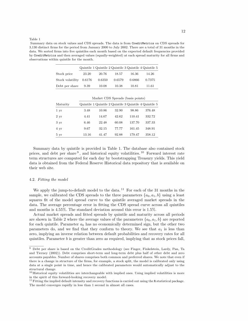
We obtained data from CreditMetrics on CDS spreads for 3,130 distinct firms forthe period from January 2000 to July 2002. The data comprise a spread curve withmaturities from 1 to 10 years derived from market data using their model. We used onlythe curve from 1 to 5 years, and incorporated half-year time steps into our analysis byinterpolating the half-year spread levels from 1 to 5 years. There are a total of 31 monthsin the data. We sorted firms into five quintiles each month based on the expected defaultfrequencies provided by CreditMetrics and then averaged values (equally-weighted) ateach spread maturity for all firms and observations within quintile for the month. Hence,we obtain an average CDS spread curve per month for each quintile.

12

Table 1Summary data on stock values and CDS spreads. The data is from CreditMetrics on CDS spreads for

3,130 distinct firms for the period from January 2000 to July 2002. There are a total of 31 months in the

data. We sorted firms into five quintiles each month based on the expected default frequencies providedby CreditMetrics and then averaged values (equally-weighted) at each spread maturity for all firms and

observations within quintile for the month.

Quintile 1 Quintile 2 Quintile 3 Quintile 4 Quintile 5

Stock price 23.20 20.76 18.57 16.36 14.26

Stock volatility 0.6176 0.6350 0.6579 0.6866 0.7375

Debt per share 9.39 10.08 10.38 10.81 11.61

Market CDS Spreads (basis points)

Maturity Quintile 1 Quintile 2 Quintile 3 Quintile 4 Quintile 5

1 yr 3.48 10.86 32.90 98.86 376.48

2 yr 4.41 14.67 42.62 110.41 332.72

3 yr 6.46 22.48 60.08 137.70 337.33

4 yr 9.67 32.15 77.77 161.45 348.91

5 yr 13.16 41.47 92.88 179.47 358.12

Summary data by quintile is provided in Table 1. The database also contained stockprices, and debt per share 9 , and historical equity volatilities. 10 Forward interest rateterm structures are computed for each day by bootstrapping Treasury yields. This yielddata is obtained from the Federal Reserve Historical data repository that is available ontheir web site.

4.2. Fitting the model

We apply the jump-to-default model to the data. 11 For each of the 31 months in thesample, we calibrated the CDS spreads to the three parameters {a0, a1, b} using a leastsquares fit of the model spread curve to the quintile averaged market spreads in thedata. The average percentage error in fitting the CDS spread curve across all quintilesand months is 4.55%. The standard deviation around this error is 1.5%.

Actual market spreads and fitted spreads by quintile and maturity across all periodsare shown in Table 2 where the average values of the parameters {a0, a1, b} are reportedfor each quintile. Parameter a0 has no economically determined sign, but the other twoparameters do, and we find that they conform to theory. We see that a1 is less thanzero, implying an inverse relation between default probabilities and recovery rates for allquintiles. Parameter b is greater than zero as required, implying that as stock prices fall,

9 Debt per share is based on the CreditGrades methodology (see Finger, Finkelstein, Lardy, Pan, Taand Tierney (2002)). Debt comprises short-term and long-term debt plus half of other debt and zero

accounts payables. Number of shares comprises both common and preferred shares. We note that even if

there is a change in structure of the firms, for example, a stock split, the model is calibrated only usingdata at a single point in time, and hence the calibrated parameters would automatically adjust to thestructural change.10Historical equity volatilities are interchangeable with implied ones. Using implied volatilities is morein the spirit of this forward-looking recovery model.11Fitting the implied default intensity and recovery functions is carried out using the R statistical package.

The model converges rapidly in less than 1 second in almost all cases.

13

Table 2Actual and fitted spread term structures. The spread values represent the averages across 31 months of

data for each quintile broken down by the maturity of the CDS contract into 1 to 5 years. The parameters

{a0, a1, b} are the three parameters for the default probability and recovery rate functions. We reportthe average of these values for the entire period by quintile.

Parameter Quintile 1 Quintile 2 Quintile 3 Quintile 4 Quintile 5

a0 2.0937 1.4679 0.9778 0.6622 7.1245

a1 -4.1005 -5.0468 -3.2557 -1.1549 -11.9068

b 1.3421 1.3503 1.2594 1.0399 0.3519

Market CDS Spreads in basis points

Maturity Quintile 1 Quintile 2 Quintile 3 Quintile 4 Quintile 5

1 yr 3.48 10.86 32.90 98.86 376.48

2 yr 4.41 14.67 42.62 110.41 332.72

3 yr 6.46 22.48 60.08 137.70 337.33

4 yr 9.67 32.15 77.77 161.45 348.91

5 yr 13.16 41.47 92.88 179.47 358.12

Fitted CDS Spreads in basis points

Maturity Quintile 1 Quintile 2 Quintile 3 Quintile 4 Quintile 5

1 yr 3.20 10.12 30.12 90.35 352.71

2 yr 4.44 14.73 43.36 117.60 342.67

3 yr 6.55 22.75 61.89 143.25 347.60

4 yr 9.81 32.62 78.77 161.64 354.06

5 yr 13.05 41.13 91.39 173.80 359.22

RMSE/Avg Spread 0.0405 0.0351 0.0451 0.0625 0.0444

Stdev 0.0126 0.0082 0.0104 0.0065 0.0191

the probability of default becomes larger. Since λ = 1/Sb, the smaller the value of b, thegreater the probability of default. As can be seen in Table 2, the value of this parameter,though non-monotonic, is much smaller for the higher (low credit quality) quintile.

4.3. Calibrated term structures

Using the data in Table 1 on the “average” firm within each quintile, we calibratedthe model. For each month and quintile, we used the calibrated values of {a0, a1, b} tocompute the term structures of forward probabilities of default and forward recovery ratesby applying equations (14) and (15). These are displayed in Figures 1 and 2 respectively.

The term structures of forward default probabilities in Figure 1 show increasing termstructures for the better quality credit qualities (quintiles 1 to 3). Quintile 4 has a humpedterm structure, and quintile 5 (the poorest credit quality) has a declining term structureof default probability. This conforms to known intuitions. For low quality firms, the short-run likelihood of default is high, and then declines, conditional on survival. Therefore,we see that the conditional forward default probabilities for Quintile 5 decline rapidly.

14

0

0.02

0.04

0.06

0.08

0.1

0.12

0.14

0.16

0.18

0.2

1 2 3 4 5Maturity (yrs)

Q1Q2Q3Q4Q5

Fig. 1. Term structure of Forward Probabilities of Default for each quintile using data averaged over

31 months (Jan 2000 to July 2002). All firms in the sample were divided into quintiles based on their

expected default frequencies (EDFs). The average CDS spread curve in each quintile is used to fitthe jump-to-default (JTD) model using the stock price and stock volatility as additional identification

data. Fitting is undertaken using a two parameter function for the forward recovery rate (φ) and a one

parameter function for the forward probability of default (λ). The overall average probability of defaultfrom all quintiles and across all months and maturities in the data is 5.86%.

Conversely, for high quality firms the short-run probability of default is low comparedto longer maturities. The average risk-neutral probability of default is 5.86% per annum(across all quintiles and maturities in the term structure). We note that expected de-fault frequencies under the statistical probability measure in prior work (see Das, Duffie,Kapadia and Saita (2007) for example) is around 1.5%, implying a ratio of risk-neutralto physical default probabilities of around 3 to 4, consistent with what is known in theliterature, e.g. Berndt, Douglas, Duffie, Ferguson and Schranz (2005).

The term structures of forward recovery rates are shown in Figure 2. Recovery termstructures show declining levels as the quality of the firms declines from quintile 1 toquintile 5. Quintile 1 recovery rates are in the 90% range, whereas the worst qualityquintile has recovery rates that drop to the 30% range. The average across all maturitiesand quintiles of the risk-neutral forward recovery rate in our data is 73.55%. The termstructures are declining, i.e. the forward recovery is lower when the firm defaults laterrather than sooner. There may be several reasons for this. First, firms that migrateslowly into default suffer greater dissipation of assets over time, whereas a firm that hasa short-term surprise default may be able to obtain greater resale values for its assets.Second, sudden defaults of high-grade names that are associated with fraud result in lossof franchise value, though the assets of the firm are still valuable and have high resalevalues. Recovery rates of the poorest quintile firms are in the range seen in the empiricalrecord. This is the quintile from which almost all defaults have historically occurred. Incontrast, surprise defaults of high quality firms are likely to result in higher recoveryrates. Finally, we note that in the Merton (1974) structural class of models, conditionalrecovery rates usually decline with maturity, since recovery in that model depends onthe firm value at maturity; conditional on default, a firm is likely to have lost more of its

15

0

0.1

0.2

0.3

0.4

0.5

0.6

0.7

0.8

0.9

1

1 2 3 4 5Maturity (yrs)

Q1Q2Q3Q4Q5

Fig. 2. Term structure of Recovery Rates for each quintile using data averaged over 31 months (Jan

2000 to July 2002). All firms in the sample were divided into quintiles based on their expected defaultfrequencies (EDFs). The average CDS spread curve in each quintile is used to fit the jump-to-default

(JTD) model using the stock price and stock volatility as additional identification data. Fitting is un-

dertaken using a two parameter function for the forward recovery rate (φ) and a one parameter functionfor the forward probability of default (λ). The overall average recovery rate from all quintiles and across

all months in the data is 73.55%.

asset value over a longer time frame.In a separate exercise, we fitted the model to the average firm for each quintile within

each month. We then averaged default probabilities and recovery rates across maturitiesand quintiles for each month to construct time series indices. The plot is shown in Figure3. Over the period from 2000 to 2002, the credit markets worsened. This is evidenced inthe increasing levels of implied probabilities of default and declining levels of recoveryrates. The time series correlation of the two series is −0.56. While this relationship isobtained for the risk-neutral measure, similar, though technically unconnected results areobtained for the statistical measure – Altman, Brady, Resti and Sironi (2005) also founda strong negative correlation using data on realized default and recovery rates. Similarlevels of negative correlation are also provided in the results of Chava, Stefanescu andTurnbull (2006).

4.4. Individual Firm Calibration

The analysis of the model using quintile-aggregated data provides only a first cutassessment that the model is a reasonable one. In practice, the model is intended forapplication to individual names. Therefore in this sub-section, we explore three liquidlytraded issuers over the period January 2000 to July 2002. The issues we examine are (a)parameter stability in the calibration of the model, (b) evolution of the term structuresof forward default probabilities and recovery rates over this time period, and (c) thestability of the model calibration to different forms of the recovery function.

16

0.035

0.037

0.039

0.041

0.043

0.045

0.047

0.049

0.051

0.053

Jan-

00

Mar

-00

May

-00

Jul-00

Sep

-00

Nov

-00

Jan-

01

Mar

-01

May

-01

Jul-01

Sep

-01

Nov

-01

Jan-

02

Mar

-02

May

-02

Jul-02

Pro

bab

ilit

y o

f d

efa

ult

(Lam

bd

a)

0.6

0.61

0.62

0.63

0.64

0.65

0.66

0.67

0.68

0.69

0.7

Reco

very r

ate

(P

hi)

AVG LAM

AVG PHI

Fig. 3. Average probability of default and recovery rates over the sample period. The Figure depicts theequally weighted average across all quintiles of the data. As credit risk increased in the economy from

2000 to 2002, we see that the probability of default increased whereas the implied recovery rate declined.

The average is taken across all maturities of the term structure at a given point in time. The correlationbetween the time series of default probability and recovery rates is −0.56.

We chose three issuers for this exercise, of low, medium and high credit risk. The threefirms are Sunoco (SUN), General Motors (GM) and Amazon (AMZN) respectively. Foreach firm month, we fitted the model to only 5 points on the average CDS spread curvefor the month, i.e. to the 1,2,3,4,5 year maturities. The calibration exercise also uses thestock price, stock volatility, and the forward interest rate curve (averages for the month).

4.4.1. Time seriesWe begin by examining the results for the low risk firm Sunoco. Figure 4 shows the

history of the 5 yr CDS spread. We see that spreads for Sunoco declined over time, eventhough the overall change for the 5 year maturity is just 25 basis points, which is verysmall. The figure also shows that the three parameters (a0, a1, b) of the λ and φ functionsare relatively stable over time. The term structures of forward default probabilities andrecovery rates are shown in Figure 5. The term structure of default probability has amildly humped shape. The term structure of recovery is declining.

The medium risk firm that we analyzed is GM, results for which are shown in Figures6 and 7. Whereas with Sunoco, the 5 year CDS spread ranged from 45 to 75 basis points,in the case of GM, the range is from 150 to 450 basis points. We note that the termstructure of CDS spreads is inverted, so that the short term spreads are higher than longterm spreads. The shape of the spread curve is indicative of the market’s concern withshort-run default. Correspondingly, we see that the parameter b is much lower than thatexperienced with Sunoco. This is also evidence in a downward sloping term structure ofdefault probability. In the case of GM, spreads increased over the time period, whereaswith Sunoco, the opposite occurred. Also, the 5 year recovery rate is much lower for GM(in the range of 20-30%) versus Sunoco (in the range of 70-80%).

17

0 5 10 15 20 25 30

45

50

55

60

65

70

5yr CDS spreads

months: 01/2000 - 07/2002

cds

spr

0 5 10 15 20 25 30

3.0

3.5

4.0

4.5

Parameter a0

months: 01/2000 - 07/2002

a0

0 5 10 15 20 25 30

-95

-90

-85

-80

-75

Parameter a1

months: 01/2000 - 07/2002

a1

0 5 10 15 20 25 30

0.95

1.05

1.15

1.25

Parameter b

months: 01/2000 - 07/2002

b

sun.dat

Fig. 4. Calibration Time Series for Sunoco. This graph shows the time series of CDS spreads andcalibrated parameters (a0, a1, b) for the period Jan 2000 to July 2002.

As an example of a firm with very high risk, we look at Amazon. Result for AMZN areshown in Figures 8 and 9. In this case, spreads ranged from 450 to 1100 basis points, andincreased rapidly over the time period as market conditions worsened. The probabilities ofdefault increased and then declined somewhat. However, in a clear indication of worseningconditions, the recovery rates declined rapidly over the time period, suggestive of a lowimplied resale value of Amazon’s assets. We see that the parameters vary over timebut in a smooth manner. In the case of all three firms, parameter evolution appears tobe quite smooth (with a range). Hence, there is some “stickiness” to the parameters,suggesting that credit model structure, even for individual firms, does not change ina drastic manner. The indication we obtain from these single-issuer analyses is thatour dynamic modeling of the term structures of default probabilities and recovery ratesappears to work well with forward interest rates, stock prices and stock volatilities asdriving state variables.

4.4.2. Alternative Recovery Function SpecificationsThe recovery model in the paper is essentially a probit function specification. To recall,

the recovery rate is modeled as φ = N(a0 + a1λ), where N(·) is the normal distributionfunction. We note that this specification ensures that the recovery rate remains boundedin the (0, 1) range.

We now examine two other specifications. These are:(i) Logit. The functional form is

φ =1

1 + exp(a0 + a1λ)

18

maturity

1

2

3

4

5

month

s (J

an 2000 -

July 2

002)

5

10

15

20

25

30

Fw

d P

Ds

0.020

0.022

0.024

0.026

0.028

0.030

sun.dat

maturity

1

2

3

4

5

month

s (J

an 2000 -

July 2

002)

5

10

15

20

25

30

Fw

d R

ecov ra

tes

0.70

0.75

0.80

0.85

0.90

0.95

sun.dat

Fig. 5. Calibration Time Series for Sunoco. This graph shows the time series of implied term structures

of forward default probabilities and recovery rates for the period Jan 2000 to July 2002.

(ii) Arctan. The functional form here is as follows:

φ =12

[arctan(a0 + a1λ)

2π

+ 1]

We note that under both these specifications as well, the recovery function producesvalues that remain in the (0, 1) interval.

We re-calibrated the model under these specifications and compared the extractedterm structures of default and recovery for all three of our sample firms. The results arepresented in Table 3. We used the calibration of the model for the month of September2001 as an illustration. We note the following features of these results. First, the fittingerror (RMSE) is very small, ranging from less than 1% of average CDS spreads (in thecase of AMZN) to 8.2% (in the arctan model for SUN). The model appears to fit betterfor poor credit quality firms than for good ones (because spreads are larger for poorfirms, the percentage error tends to be lower). Second, the calibrated term structuresof default probabilities and recovery rates are similar across the three recovery functionspecifications. They are the closest for AMZN and least similar for SUN, although notthat different. Therefore, model specification does not appear to be much of an issue. Ofcourse, the fitted parameters are different, but the fact that the models deliver similar

19

0 5 10 15 20 25 30

200

300

400

5yr CDS spreads

months: 01/2000 - 07/2002

cds

spr

0 5 10 15 20 25 30

68

10

12

Parameter a0

months: 01/2000 - 07/2002

a0

0 5 10 15 20 25 30

-40

-30

-20

-10

Parameter a1

months: 01/2000 - 07/2002

a1

0 5 10 15 20 25 30

0.100.150.200.250.30

Parameter b

months: 01/2000 - 07/2002

b

gm.dat

Fig. 6. Calibration Time Series for General Motors. This graph shows the time series of CDS spreads

and calibrated parameters (a0, a1, b) for the period Jan 2000 to July 2002.

results suggests that the framework is general and may be implemented in differentways. The overall conclusion is that the model is insensitive to the parametric form ofthe recovery function, and tends to fit the data better for high risk firms than low riskones.

4.4.3. Calibration sensitivity to changes in inputsWe now examine whether the implied framework is overly sensitive to the inputs. Are

the extracted term structures of default and recovery so sensitive to the inputs that smallchanges in the inputs result in dramatic changes in the resultant term structures?

To assess this question, we used the calibration setting for our three sample firms in themonth of September 2001, as before. We changed each input to the model by increasingthem individually by 10% and then examined the resultant changes in the calibratedparameters and the term structures. The results are portrayed in Table 4. Across allthe experiments conducted, for the low and medium risk firm cases, the sensitivity ofthe calibrated parameters and the implied term structures does not display any suddenchanges. In fact, the change in implied values does not exceed 10%. For the high risk firm,we do see some change in the calibrated parameters for the change in stock price andvolatility. This indicates that at very low stock price and high volatility levels, the termstructures of default probabilities and recovery rates do seem to be sensitive to changesin inputs, resulting in changes in the calibrated parameters as well. Overall, the evidencemostly suggests that the model framework is very stable in the calibration process.

20

maturity

1

2

3

4

5

month

s (J

an 2000 -

July 2

002)

5

10

15

20

25

30

Fw

d P

Ds

0.1

0.2

0.3

0.4

0.5

gm.dat

maturity

1

2

3

4

5

month

s (J

an 2000 -

July 2

002)

5

10

15

20

25

30

Fw

d R

ecov ra

tes

0.2

0.4

0.6

0.8

gm.dat

Fig. 7. Calibration Time Series for General Motors. This graph shows the time series of implied term

structures of forward default probabilities and recovery rates for the period Jan 2000 to July 2002.

4.4.4. Calibrating multiple spread curvesFor a single firm, there may be multiple debt issues with different features. For exam-

ple, the debt tranches may differ in their seniority. CDS contracts written on differentreference instruments of the same firm will have the same default probability term struc-ture, but different recovery rate term structures. The market for LCDS is a good exampleof derivatives on multiple debt tranches, as most LCDS names also have traded bondCDS.

It is possible to calibrate our model to multiple debt tranches of the same firm. With-out loss of generality, assume that there are two debt tranches in the firm. Calibra-tion is undertaken by fitting both term structures of CDS spreads to five parameters:{a01, a11, a02, a12, b}, where alj is the parameter al, l = {0, 1} for the j-th term structureof credit spreads. Of course, since the term structure of default probabilities is the sameacross the debt tranches, only a common parameter b is necessary.

To illustrate, we take the example of Amazon for September 2001. Using the same dataas in the previous subsection, we created two term structures of CDS spreads by settingone term structure to be higher than that of the original data and setting the secondone to be lower. One may imagine the latter term structure to relate to debt with higherseniority than the former term structure. Each term structure is annual and hence we

21

0 5 10 15 20 25 30

500

700

900

1100

5yr CDS spreads

months: 01/2000 - 07/2002

cds

spr

0 5 10 15 20 25 30

-2-1

01

23

Parameter a0

months: 01/2000 - 07/2002

a0

0 5 10 15 20 25 30

-15

-10

-50

Parameter a1

months: 01/2000 - 07/2002

a1

0 5 10 15 20 25 30

0.6

0.7

0.8

0.9

1.0

1.1

Parameter b

months: 01/2000 - 07/2002

b

amzn.dat

Fig. 8. Calibration Time Series for Amazon. This graph shows the time series of CDS spreads and

calibrated parameters (a0, a1, b) for the period Jan 2000 to July 2002.

calibrate ten observations to five parameters by minimizing the root mean-squared error(RMSE) across both term structures. Convergence is rapid and results in a single termstructure of default probabilities and two term structures of recovery rates. The inputsand outputs of this calibration exercise are shown in Table 5. As expected, the higherquality tranche results in recovery rates that are higher than that of the lower qualitytranche.

Analogously, it may be of interest to calibrate the spread curves of multiple issuersjointly such that they all have the same default probability term structure, but differentrecovery term structures. The approach would be the same – the parameter b is will bethe same across issuers, but separate parameters will be used for the individual recoveryterm structures.

5. Discussion

There is no extant model for determining forward looking recovery rates, even thoughrecovery rates are required in the pricing of almost all credit derivative products. Thismarket deficiency stems from an identification problem emanating from the mathematicalstructure of credit products. Market participants have usually imposed recovery rates of40% or 50% (for U.S. corporates) in an ad-hoc manner in their pricing models.

The paper remedies this shortcoming of existing models. We develop a flexible jump-to-default model that uses additional data, the stock price S and stock volatility σin conjunction with credit spreads to identify not just the implied values of defaultprobability λ and recovery rate φ, but instead, the parameterized functional forms of

22

maturity

1

2

3

4

5

month

s (J

an 2000 -

July 2

002)

5

10

15

20

25

30

Fw

d P

Ds

0.05

0.10

0.15

amzn.dat

maturity

1

2

3

4

5

month

s (J

an 2000 -

July 2

002)

5

10

15

20

25

30

Fw

d R

ecov ra

tes

0.2

0.4

0.6

0.8

amzn.dat

Fig. 9. Calibration Time Series for Amazon. This graph shows the time series of implied term structures

of forward default probabilities and recovery rates for the period Jan 2000 to July 2002.

these two inputs. The model in this paper is parsimonious and requires the calibrationof only three parameters {a0, a1, b}.

We illustrate the application of the model using average firm data on CDS spreadcurves for 5 quintiles over 31 months in the period from January 2000 to July 2002. Wecalibrate the model for each quintile and month, and then use the calibrated parametersto identify the risk-neutral term structures of forward default probabilities and recoveryrates.

We also examined the behavior of the model on low, medium and high risk firms, withupward and downward sloping credit spread term structures. Many useful results areobtained. First, the model calibrate very well to individual firms, with very low mean-squared errors. Second, fitting the model month by month, we find that there is stabilityin the estimated parameters. Hence, the parameters do change in a smooth mannerover time, and the dynamics of the extracted term structures of default probability andrecovery are driven by changes in the state variables (equity prices and volatilities).Third, we assessed the model for different recovery rate specifications and found thatthe extracted term structures are robust to changes in model specification. Fourth, wedemonstrate that the calibration of the model is not sensitive to small changes in theinputs. Hence, the mathematical framework of the model is stable. Fifth, we extended the

23

Table 3Calibration of the model for alternative recovery function specifications. For each of the three illustrative

firms - SUN, GM, AMZN - we calibrated the model for September 2001 using three specifications for

the recovery function: (a) Probit: φ = N(a0 + a1λ), (b) Logit: φ = 11+exp(a0+a1λ)

, and (c) Arctan:

φ = 12

[arctan(a0 + a1λ) 2

π+ 1]. The results are presented in the three panels below, one for each firm.

The market spreads are shown, along with the fitted spreads, so as to give an idea of the quality offit. For each recovery function, we report the fitted spread and the calibrated term structure of forward

default probabilities and recovery rates. The percentage RMSE is also reported (it is the root mean-

squared error divided by the average CDS spread across maturities for the month). The other inputs areprovided in Table 4.

SUN Probit Model: %RMSE=4.8 Logit Model: %RMSE=5.02 Arctan Model: %RMSE=8.17

Maturity (yrs) Mkt CDS spr Fitted Spr Fwd PD Fwd Recov Fitted Spr Fwd PD Fwd Recov Fitted Spr Fwd PD Fwd Recov

1 6.74 6.23 0.0278 0.9776 6.70 0.0252 0.9734 9.97 0.0314 0.9683

2 15.40 14.99 0.0285 0.9100 14.08 0.0261 0.9124 12.14 0.0319 0.9305

3 28.98 31.08 0.0287 0.8209 31.28 0.0265 0.8094 31.31 0.0318 0.8808

4 43.08 43.89 0.0285 0.7844 43.51 0.0265 0.7853 43.17 0.0312 0.7934

5 55.99 53.78 0.0278 0.7438 53.97 0.0261 0.7349 54.03 0.0302 0.7305

Parameters (a0, a1, b): 4.178 -78.189 0.994 -7.541 156.279 1.021 21.344 -360.64 0.959

GM Probit Model: %RMSE=3.4 Logit Model: %RMSE=3.8 Arctan Model: %RMSE=5.1

Maturity (yrs) Mkt CDS spr Fitted Spr Fwd PD Fwd Recov Fitted Spr Fwd PD Fwd Recov Fitted Spr Fwd PD Fwd Recov

1 1038.12 1045.11 0.2816 0.6288 1045.67 0.2753 0.6202 1049.91 0.2465 0.5741

2 735.34 697.81 0.1869 0.6590 691.93 0.1845 0.6673 674.56 0.1723 0.7040

3 532.72 536.99 0.1287 0.5332 538.19 0.1280 0.5353 545.66 0.1239 0.5481

4 447.25 463.44 0.0911 0.4015 465.54 0.0913 0.4080 468.90 0.0912 0.4486

5 398.49 421.44 0.0661 0.3102 422.58 0.0666 0.3192 424.08 0.0685 0.3600

Parameters (a0, a1, b): 12.724 -44.026 0.248 -23.330 82.950 0.254 95.694 -387.23 0.282

AMZN Probit Model: %RMSE=0.1 Logit Model: %RMSE=0.1 Arctan Model: %RMSE=0.1

Maturity (yrs) Mkt CDS spr Fitted Spr Fwd PD Fwd Recov Fitted Spr Fwd PD Fwd Recov Fitted Spr Fwd PD Fwd Recov

1 749.92 749.86 0.1381 0.4571 749.87 0.1382 0.4576 749.86 0.1381 0.4572

2 942.44 942.52 0.1876 0.3957 942.50 0.1876 0.3959 942.51 0.1876 0.3957

3 1048.50 1048.66 0.1713 0.3102 1048.69 0.1713 0.3103 1048.67 0.1713 0.3102

4 1054.55 1054.48 0.1014 0.2307 1054.49 0.1014 0.2308 1054.48 0.1014 0.2307

5 1071.10 1070.98 0.0910 0.1845 1070.99 0.0909 0.1845 1070.98 0.0910 0.1845

Parameters (a0, a1, b): -0.116 0.063 0.931 0.183 -0.094 0.930 -0.146 0.079 0.931

model to fitting multiple debt tranches of the same issuer, such that the term structureof default probabilities remains the same across tranches, yet we obtain multiple termstructures of recovery rates, one for each debt tranche. The same approach also works toextend the model to fitting multiple issuers (within the same rating class for example)simultaneously to better make use of the information across issuers.

A natural question that arises in this class of models is whether the model dependscritically on integration of the equity and credit markets (see Kapadia and Pu (2008)for evidence of weak integration). We note that integration of markets is a very strongcondition that is sufficient but not necessary for our framework. The model uses the stockprice and volatility as state variables that drive the dynamics of default and recovery. Aslong as there is an established empirical link between the dynamics of equity and credit

24

Table 4Sensitivity of implied term structures of forward default probabilities (FwdPD) and recovery rates

(FwdRecov) to changes in input variables. The Probit specification for recovery rates is used. Keeping

forward rates and CDS spreads fixed (initial data), the base case inputs and calibrated term structuresof default probabilities and recovery rates are presented first. In the lower half of the panel for each firm,

we show the input stock price and volatility, as well as the three parameters (a0, a1, b) as calibrated for

best fit. The fitting error (RMSE as a percentage of average CDS spread) is also reported. Calibration isthen undertaken after shifting the stock price up by 10%. Results are reported under the heading “Stock

Shift”. Next, the “Volatility Shift” case shows the calibration results when volatility is shifted up by10%. Finally, the “CDS Spr Shift” columns show the results when the entire spread curve experiences a

parallel upward shift of 10%.

SUN Initial Data Base Case Stock Shift Volatility Shift CDS Spr Shift

T FwdRt Mkt Spr FwdPD FwdRecov FwdPD FwdRecov FwdPD FwdRecov FwdPD FwdRecov

1 0.0282 6.74 0.0278 0.9776 0.0288 0.9787 0.0209 0.9662 0.0297 0.9782

2 0.0341 15.40 0.0285 0.9100 0.0293 0.9101 0.0225 0.9049 0.0303 0.9041

3 0.0412 28.98 0.0287 0.8209 0.0295 0.8204 0.0238 0.8177 0.0304 0.8095

4 0.0478 43.08 0.0285 0.7844 0.0291 0.7837 0.0246 0.7739 0.0300 0.7776

5 0.0545 55.99 0.0278 0.7438 0.0283 0.7424 0.0250 0.7372 0.0291 0.7322

Inputs Params Inputs Params Inputs Params Inputs Params

Stk Price a0 36.293 4.179 39.922 4.339 36.293 3.328 36.293 4.394

Stk Vol a1 0.338 -78.190 0.338 -80.220 0.372 -71.636 0.338 -79.919

b 0.994 0.958 1.073 0.974

RMSE% 4.808 5.062 2.304 6.071

GM Initial Data Base Case Stock Shift Volatility Shift CDS Spr Shift

T FwdRt Mkt Spr FwdPD FwdRecov FwdPD FwdRecov FwdPD FwdRecov FwdPD FwdRecov

1 0.0282 1038.12 0.2816 0.6288 0.2819 0.6292 0.3023 0.6542 0.2847 0.5961

2 0.0341 735.34 0.1869 0.6590 0.1873 0.6588 0.1952 0.6527 0.1881 0.6501

3 0.0412 532.72 0.1287 0.5332 0.1290 0.5329 0.1310 0.5041 0.1290 0.5317

4 0.0478 447.25 0.0911 0.4015 0.0914 0.4006 0.0907 0.3697 0.0911 0.3974

5 0.0545 398.49 0.0661 0.3102 0.0663 0.3089 0.0644 0.2798 0.0659 0.3052

Inputs Params Inputs Params Inputs Params Inputs Params

Stk price a0 87.256 12.726 95.982 12.965 87.256 13.602 87.256 13.026

Stk Vol a1 0.324 -44.034 0.324 -44.828 0.356 -43.678 0.324 -44.905

b 0.248 0.242 0.229 0.245

RMSE% 3.362 3.345 4.094 3.251

AMZN Initial Data Base Case Stock Shift Volatility Shift CDS Spr Shift

T FwdRt Mkt Spr FwdPD FwdRecov FwdPD FwdRecov FwdPD FwdRecov FwdPD FwdRecov

1 0.0282 749.92 0.1381 0.4571 0.1196 0.3722 0.1750 0.5729 0.1382 0.4030

2 0.0341 942.44 0.1876 0.3957 0.1737 0.3460 0.2180 0.4608 0.1876 0.3491

3 0.0412 1048.50 0.1713 0.3102 0.1734 0.2872 0.1766 0.3363 0.1713 0.2738

4 0.0478 1054.55 0.1014 0.2307 0.1048 0.2096 0.1013 0.2423 0.1014 0.2035

5 0.0545 1071.10 0.0910 0.1845 0.0938 0.1711 0.0856 0.1840 0.0910 0.1628

Inputs Params Inputs Params Inputs Params Inputs Params

Stk price a0 7.756 -0.116 8.531 -0.409 7.756 0.255 7.756 -0.255

Stk Vol a1 0.972 0.063 0.972 0.690 1.069 -0.406 0.972 0.069

b 0.931 0.961 0.805 0.930

RMSE% 0.011 0.286 0.308 0.011

25

Table 5Simultaneous calibration of multiple CDS spread curves. CDS contracts written on different reference

instruments of the same firm will have the same default probability term structure, but different recovery

rate term structures. We take the example of Amazon for September 2001. We created two term structuresof CDS spreads by setting one term structure to be higher than that of the original data and we set

the second one to be lower. Each term structure is annual and we calibrate ten observations to fiveparameters. Calibration is undertaken by fitting both term structures of CDS spreads to five parameters:

{a01, a11, a02, a12, b}, where alj is the parameter al for the j-th term structure. Since the term structure

of default probabilities is the same across the debt tranches, only a common parameter b is necessary.The screen shot shows the fit of the model in Excel. The input spread curves are denoted “MktSpr1”

and “MktSpr2”. The fitted spread curves are “CDSspr”. The forward default probability and recovery

rate curves are denoted “FwdPD” and “FwdRec” respectively.

Inputs Outputs

Maturity (T ) Fwd Rate MktSpr1 MktSpr2 FwdPD FwdRec1 FwdRec2

1 0.0226 899.06 599.38 0.1735 0.4818 0.6541

2 0.0273 1130.93 753.95 0.2015 0.3712 0.5230

3 0.0329 1258.20 838.80 0.1647 0.2762 0.3914

4 0.0383 1265.46 843.64 0.1025 0.2114 0.2941

4 0.0436 1285.32 856.88 0.0838 0.1629 0.2272

Inputs: S = 7.756, σ = 0.972, h = 1

Parameters: a01 = 0.161, a02 = 0.533, a11 = −1.189, a12 = −0.788, b = 0.809

risk, the model is on a good footing. Indeed, the same is assumed in all structural modelsof default risk, and we have shown this linkage theoretically in the paper. There is agrowing body of empirical evidence that CDS spreads are well-related to equity dynamics,as in the work of Berndt, Douglas, Duffie, Ferguson and Schranz (2005), Duffie, Saita andWang (2005), and Das and Hanouna (2009). Another body of evidence shows that thatdefault and recovery prediction models are also well grounded on distance-to-default, ameasure of credit risk extracted from equity prices and volatilities (see Finger, Finkelstein,Lardy, Pan, Ta and Tierney (2002); Gupton and Stein (2005); Jarrow (2001); Sobehart,Stein, Mikityanskaya and Li (2000); and Das, Hanouna and Sarin (2006)). Nevertheless,the model is agnostic as to the state variable that may be used to drive credit spreaddynamics. Instead of equity, any other variable that relates to credit risk may be usedsuch as macroeconomic variables and ratings, as long as there are sufficient inputs thatallow the variable’s dynamics to be represented on the model tree.

The model is flexible in the manner in which it may be calibrated. Instead of equity,options may be used to calibrate the model. We note that the volatility input to the modelcurrently captures the information from options. However, one deficiency of the modelis that it does not use the information in the option smile, which is partially related tocredit risk (it is easy to show that in a jump-to-default model of equity, a negative skewon tree from the default jump results in an implied volatility skew). To accommodate thevolatility skew in our model we would need to change the pricing tree from the currentone, i.e. the Cox, Ross and Rubinstein (1979) tree, to the local volatility tree model ofDerman and Kani (1994). This would enhance the complexity of the model appreciablyand we leave it for future research. However, this is an important extension, becauseit allows the entire volatility surface to be used in the calibration exercise, raising theinformation content of the model.

Given that the model is easy to understand and calibrate, it may be used to further thedevelopment of credit derivatives indexed to recovery rates, such as recovery swaps anddigital default swaps. It will also provide useful guidance to regulators in their recovery

26

specifications for the implementation of Basel II.

Appendix A. Appendix: Constant Recovery Rates

In practice, a common assumption is to fix the recovery rate to a known constant. Ifwe impose the condition that φj ≡ φ, ∀j, it eliminates N parameters, leaving only the Ndefault intensities, λj . Now, we have N equations with as many parameters, which maybe identified in a recursive manner using bootstrapping. To establish ideas, we detailsome of the bootstrapping procedure.

Starting with the one-period (N = 1) default swap, with a premium C1 per annum,we equate payments on the swap as follows:

A1 =B1

C1 h Q(T0)D(T1) =(1− e−λ1h

)D(T1)(1− φ)

C1 h =(1− e−λ1h

)(1− φ)

This results in an identification of λ1, which is:

λ1 = − 1h

ln[

1− φ− C1 h

1− φ

], (A.1)

which also provides the survival function for the first period, i.e. Q(T1) = exp(−λ1 h).We now use the 2-period default swap to extract the intensity for the second period.

The premium for this swap is denoted as C2. We set A2 = B2 and obtain the followingequation which may be solved for λ2.

C2 h

2∑j=1

Q(Tj−1)D(Tj) =2∑j=1

Q(Tj−1)(1− e−λjh

)D(Tj)(1− φ) (A.2)

Expanding this equation, we have

C2 h {Q(T0)D(T1) +Q(T1)D(T2)}=Q(T0)

(1− e−λ1h

)D(T1)(1− φ)

+Q(T1)(1− e−λ2h

)D(T2)(1− φ)

Re-arranging this equation delivers the value of λ2, i.e.

λ2 =− 1h

ln[L1/L2] (A.3)

L1 ≡Q(T0)(1− e−λ1h

)D(T1)(1− φ)

+Q(T1)D(T2)(1− φ)− C2 h [D(T1) +Q(T1)D(T2)] (A.4)

L2 ≡Q(T1)D(T2)[1− φ] (A.5)

and we also note that Q(T0) = 1.In general, we may now write down the expression for the kth default intensity:

λk =

ln

[Q(Tk−1)D(Tk)(1−φ)+

∑k−1

j=1Gj−Ck h

∑k

j=1Hj

Q(Tk−1)D(Tk)(1−φ)

]−h

(A.6)

27

Gj ≡Q(Tj−1)(1− e−λjh

)D(Tj)(1− φ) (A.7)

Hj ≡Q(Tj−1)D(Tj) (A.8)

Thus, we begin with λ1 and through a process of bootstrapping, we arrive at all λj , j =1, 2, . . . , N .

Appendix B. Time-Dependent Recovery Rates

The analysis in the previous appendix is easily extended to the case where recoveryrates are different in each period, i.e. we are given a vector of φjs. The bootstrappingprocedure remains the same, and the general form of the intensity extraction equationbecomes (for all k)

λk =−1

hln

[Q(Tk−1)D(Tk)(1− φj) +

∑k−1

j=1Gj − Ck h

∑k

j=1Hj

Q(Tk−1)D(Tk)(1− φj)

](B.1)

Gj ≡Q(Tj−1)(1− e−λjh

)D(Tj)(1− φj) (B.2)

Hj ≡Q(Tj−1)D(Tj) (B.3)

This is the same as equation (A.6) where the constant φ is replaced by maturity-specificφjs.

References

Acharya, V., Bharath, S., Srinivasan, A., 2007. Does Industry-wide Distress Affect De-faulted Firms? - Evidence from Creditor Recoveries. Journal of Financial Economics85(3), 787-821.

Altman, E., Fanjul. G., 2004. Defaults and Returns in the High-Yield Bond Market:Analysis through 2003, NYU Salomon Center, working paper.

Altman, E., Resti, A., Sironi, A., 2005. Default Recovery rates in Credit Risk Modeling:A Review of the Literature and Empirical Evidence, Journal of Finance Literature 1,21-45.

Altman, E., Brady, B., Resti, A., Sironi, A., 2005. The Link between Default and RecoveryRates: Theory, Empirical Evidence and Implications, Journal of Business 78, 2203-2228.

Bakshi, G., Madan, D., Zhang, F., 2001. Recovery in Default Risk Modeling: TheoreticalFoundations and Empirical Applications, working paper, University of Maryland.

Berd A.M., 2005. Recovery Swaps, Journal of Credit Risk 1(3), 1-10.Berndt A., Douglas, R., Duffie, D., Ferguson, M., Schranz, D., 2005. Measuring Default-

Risk Premia from Default Swap Rates and EDFs, Working paper, Graduate School ofBusiness, Stanford University.

Carey, M., Gordy, M., 2004. Measuring Systematic Risk in Recovery on Defaulted DebtI: Firm-Level Ultimate LGDs, Working paper, Federal Reserve Board.

Chan-Lau, J.A., 2008. Anticipating Credit Events using Credit Default Swaps, with anApplication to Sovereign Debt Crisis, Credit Risk: Models, Derivatives, and Manage-ment, editor: Niklas Wagner, CRC Press; (originally published as IMFworking paper3/106, 2003).

Chava, S., Jarrow, R., 2004. Bankruptcy Prediction with Industry Effects,” Review ofFinance 8, 537-569.

Chava, S., Stefanescu, C., Turnbull, S.M., 2006. Modeling Expected Loss with Unobserv-able Heterogeneity, working paper, University of Houston.

28

Christensen, J., 2005. Joint Estimation of Default and Recovery Risk: A SimulationStudy, Working paper, Copenhagen Business School.

Cox, J., Ross, A., Rubinstein, M., 1979. Option Pricing: A Simplified Approach, Journalof Financial Economics, v7, 229-263.

Das, S., Sundaram, R., 2007. An Integrated Model for Hybrid Securities, ManagementScience 53, 1439-1451.

Das, S., Freed, L., Geng, G., Kapadia, N., 2001. Correlated Default Risk, Journal ofFixed Income, Fall, 7-32.

Das, S., Duffie, D., Kapadia, N., Saita, L., 2007. Common Failings: How Corporate De-faults are Correlated, Journal of Finance 62, 93-117.

Das, S., Hanouna, P., 2009. Hedging Credit: Equity Liquidity Matters, Journal of Finan-cial Intermediation 18(1), 112-123.

Das, S., Hanouna, P., Sarin, A., 2006. Back to Basics: Fundamentals-Based versusMarket-Based Cross-Sectional Models of CDS Spreads, Journal of Banking and Fi-nance 33, 719-730.

Derman, E., Kani, I., 1994. The Volatility Smile and its Implied Tree, QuantitativeStrategies Research Notes, Goldman Sachs.

Duffie, D., 1999. Credit Swap Valuation, Financial Analysts Journal, January-February,73-87.

Duffie, D., Singleton, K., 1999. Modeling Term Structures of Defaultable Bonds, Reviewof Financial Studies 12, pp. 687-720.

Duffie, D., Saita, L., Wang, K., 2005. Multi-Period Corporate Default Prediction withStochastic Covariates, Journal of Financial Economics 83, 635-665.

Dumas, B., Fleming, J., Whaley, R., 1998. Implied Volatility Functions: Empirical Tests,Journal of Finance 53(6), 2059-2106.

Finger, C., Finkelstein, V., Lardy, J-P., Pan, G., Ta, T., Tierney, J., 2002. CreditGradesTechnical Document, RiskMetrics.

Guo, X., Jarrow, R., Zeng, Y., 2005. Modeling the Recovery Rate in a Reduced FormModel, Mathematical Finance 19(1), 73-97.

Gupton, G., Stein, R., 2005. LossCalcv2:Dynamic Prediction of LGD, Working paper,Moodys.

Hu, W., 2004. Applying the MLE Analysis on the Recovery Rate Modeling of US Cor-porate Bonds, Master’s Thesis in Financial Engineering, UC Berkeley.

Jarrow, R., 2001. Default Parameter Estimation using Market Prices, Financial AnalystsJournal 57(5), 75-92.

Jarrow, R.A., Turnbull, S.M., 1995. Pricing Derivatives on Financial Securities Subjectto Credit Risk, Journal of Finance 50(1), 53-85.

Jarrow, R.A., Lando, D., Turnbull, S.M., 1997. A Markov model for the term structureof credit risk spreads, Review of Financial Studies 10, 481-523.

Jarrow, R., Protter, P., 2004. Structural vs Reduced Form Models: A New InformationBased Perspective, Journal of Investment Management v2(2), 34-43.

Levy, A., Hu, Z., 2006. Incorporating Systematic Risk in Recovery: Theory and Evidence,Working paper, Moodys KMV.

Kapadia, N., Pu, X., 2008. Limited Arbitrage between Equity and Credit Markets, Work-ing paper, University of Massachusetts, Amherst.

Karoui, L., 2005. Modeling the Term Structure of Defaultable Bonds under RecoveryRisk, Working paper, McGill University.

Leland, H. E., 1994. Corporate Debt Value, Bond Covenants and Optimal Capital Struc-ture, Journal of Finance 49(4), 1213-1252.

Leland, H., Toft, K., 1996. Optimal Capital Structure, Endogenous Bankruptcy, and theTerm Structure of Credit Spreads, Journal of Finance 51(3), 987-1019.

29

Longstaff, F.A., Schwartz, E., 1995. A Simple Approach to Valuing Risky Fixed andFloating Rate Debt, Journal of Finance 50(3), 789-819.

Madan, D., Unal, H., 1995. Pricing the Risks of Default, Review of Derivatives Research2, 121-160.

Madan, D., Guntay, L., Unal, H., 2003. Pricing the Risk of Recovery in Default withAPR Violation, Journal of Banking and Finance 27(6), 1001-1218.

Merton, R. C., 1974. On the Pricing of Corporate Debt: The Risk Structure of InterestRates, The Journal of Finance 29, 449-470.

Pan, J., Singleton, K., 2008. Default and Recovery Implicit in the Term Structure ofSovereign CDS Spreads, Journal of Finance 63, 2345-2384.

Samuelson, P., 1972. Mathematics of Speculative Price, in: R.H. Day and S.M. Robin-son, eds, Mathematical Topics in Economic Theory and Computation, PA: Society forIndustrial and Applied Mathematics, Reprinted in SIAM Review 15, 1973, 1-42.

Schuermann, T., 2005. What do we know about Loss Given Default? in: Altman, E., Resti,A., Sironi, A., (Eds.), Recovery Risk: The Next Challenge in Credit Risk Management,Risk Books, London.

Sobehart, J., Stein, R., Mikityanskaya, V., Li, L., 2000. Moodys Public Firm Risk Model:A Hybrid Approach To Modeling Short Term Default Risk, Moodys Investors Service,Global Credit Research, Rating Methodology, March.

Song, J., 2007. Loss Given Default Implied by Cross-sectional No Arbitrage, Workingpaper, Columbia University.

Truck, S., Harpainter, S., Rachev, S., 2005. A Note on Forecasting Aggregate Recov-ery Rates with Macroeconomic Variables, Working paper, Institut fur Statistik undMathematische Wirtschaftstheorie, Universitat Karlsruhe.

Zhang, F., 2003. What Did the Credit Market Expect of Argentina Default? Evidencefrom Default Swap Data, working paper, Federal Reserve Board.