importance of networks in biology (look at stuff in google). use cases 57 8.1 biological case study
TRANSCRIPT

CellstormA bioinformatics software system to visualize subcellular
networks
Ana Neves
A thesis submitted in partial fulfillmentof the requirements for the degree of
Master of Science in the Department ofComputer Science, New York University
April 25, 2007
Approved: __________________________________________
Professor Dennis Shasha, Research Advisor

Approved: __________________________________________
Professor Zvi Kedem, Second Reader
Acknowledgements
I want to gratefully thank all the people who supported me during
my thesis project. I want to give a very special thank you to my research
advisor, Professor Dennis Shasha, for all his guidance and support. I want
to thank Chris Poultney who gave me highly qualified help and directions
for Cellstorm design and implementation. Thanks go also to Manpreet
Katari who gave me great support in the biology area and was always
available to answer my questions. I want to thank in general to all the great
researchers from the plant biology lab of Gloria Coruzzi who have helped
me during the thesis project. Finally, I want to thank my family and my
husband Andre Neves for all the patience and encouraging during the
periods of work.
2

©
Ana Neves
All Rights Reserved, 2007
Contents
1. INTRODUCTION ..................................................................................................................................... 4
2. BIOLOGICAL NETWORKS .................................................................................................................... 6
3. RELATED WORK .................................................................................................................................. 11
3.1. CYTOSCAPE ..................................................................................................................................... 11
Viewing and Filtering a Network ................................................................................................. 11 Combining Interaction and Expression Data ........................................................................... 12 Comparison with Cellstorm .......................................................................................................... 12
3.2. MAPMAN ....................................................................................................................................... 14
Comparison with Cellstorm .......................................................................................................... 16 3.3. PATHWAY STUDIO ............................................................................................................................ 17
Pathway visualization .................................................................................................................... 17 Comparison with Cellstorm .......................................................................................................... 17
3.4. SUNGEAR ........................................................................................................................................ 19
Comparison with Cellstorm .......................................................................................................... 20
4. CELLSTORM INTERFACE .................................................................................................................. 21
4.1. SUBCOMPONENTS .............................................................................................................................. 22
4.2. ZOOMING ........................................................................................................................................ 26
4.3. NETWORKS AND LINKS ...................................................................................................................... 29
5. CELLSTORM DESIGN .......................................................................................................................... 33
5.1 DATA ............................................................................................................................................ 34
5.1.1 Gene Ontology ....................................................................................................................... 35 5.1.2 Files and formatting ............................................................................................................. 36
5.2 MODULES ........................................................................................................................................ 38
5.3 PROGRAM STRUCTURE ........................................................................................................................ 40
6. CELLSTORM IMPLEMENTATION .................................................................................................... 41
6.1 CELLSTORM MAJOR DATA STRUCTURES .................................................................................................. 41
6.2 CELLSTORM MAJOR GRAPHICAL COMPONENTS .......................................................................................... 44
6.3 CELLSTORM MAJOR ALGORITHMS ....................................................................................................... 45
6.3.1. Subcomponent placement algorithm .............................................................................. 45 6.3.2. Drawing highways – thickness and quadratic curves ................................................ 48
7. CELLSTORM INTEGRATION ............................................................................................................ 55
3

8. USE CASES ............................................................................................................................................. 57
8.1 BIOLOGICAL CASE STUDY .................................................................................................................... 57
8.2. NON- BIOLOGICAL CASE STUDY ........................................................................................................... 60
9. CONCLUSION AND FUTURE WORK .............................................................................................. 63
10. REFERENCES ....................................................................................................................................... 65
1. Introduction
In the last few decades a lot has been done with the use of
computers in biological research. Information science has been applied to
biology to produce the field called Bioinformatics . Bioinformatics is now
one of the most rapidly growing areas of biological science, combining the
questions of computer science with those of biological research. The
methods of bioinformatics are being used in different fields such as
genetics, biochemistry, molecular biology, evolutionary science, cell
studies, clinical research, and field biology.
With the genomics revolution, biologists now spend much of their
time using computational tools to help them browse through the large
database of genes, proteins, and interactions. However, the access to
biological databases is not quite enough. One of the reasons is that
biologists must be able to manage and analyze large amounts of data
obtained from different sources, and therefore they have a great need for
data visualization and analysis tools.
4

Cellstorm is a bioinformatics software system that can be used by
biologists to visualize and analyze large amounts of genes’ data. Cellstorm
allows a rapid visualization of genes and networks’ interactions among the
cellular component.
Given a list of genes, an interesting problem is to know where they
located and what are the subcomponents where they are mostly expressed.
Biologists have the data needed to answer this question but a manual
process would be very time consuming. With Cellstorm we can get this
answer in a few seconds. Another interesting problem is to know how the
genes relate to each other. Cellstorm uses data from biological networks
(please refer to next chapter to see more about biological networks) to
display connections between sub- cellular components.
In sum, Cellstorm is a graphical display of genomic data where the
goal is to visualize the position of genes within a cell in terms of their sub-
cellular location and to visualize networks of various types as “highways”.
Although Cellstorm is mainly targeted for biologists, it can be used
in many other different fields. Cellstorm makes as few assumptions as
possible about the data it’s displaying, it doesn’t know, or care, if it’s
working with biological data. Cellstorm is a generic tool that avoids
building in data - specific assumptions and therefore can analyze large
amounts of data of completely different sources and fields.
5

2. Biological Networks
Biological networks facilitate the understanding of the cell’s
functional organization. Post genomic research aims to systematically
catalogue molecules and their interactions within a living cell. Indeed it is
very important to understand how these molecules and the interactions
between them determine the cell’s functional organization. Advances in
network biology indicate that cellular networks are governed by universal
laws.
For over a century, reductionism has provided knowledge about
individual cellular components and their functions, however it is clear that
a discrete biological function can only rarely be attributed to an individual
molecule. Most biological characteristics arise from complex interactions
6

between the cell’s numerous constituents, such as proteins, DNA, RNA and
small molecules.
It is increasingly recognized that complex systems cannot be
described in a reductionist view. A challenge for biology is to understand
the structure and the dynamics of the complex intracellular web of
interactions that contribute to the structure and function of the living cell.
Understanding the behavior of such systems starts with understanding the
topology of the corresponding network. Topological information is
fundamental in constructing realistic models for the function of the
network.
There are several types of networks, including protein - protein
interaction, metabolic, signaling and transcription - regulatory networks.
None of these networks are independent, instead they form a “network of
networks” which is going to be responsible for the behavior of the cell.
The cell’s behavior emerges from the activity of many components
that interact with each other through pair- wise interactions. The
components are just a series of nodes that are connected to each other by
links, with each link representing the interactions between two
components. The network is mainly formed by the nodes and links
together. In a more formal mathematical language one can say that a
network is just a graph (see figure 1).
7

Figure 1: Undirected and Directed networks
As we can see from figure 1, depending on the nature of interactions,
networks can be directed or undirected. For directed networks, the
interaction has a well- defined direction, for example the direction of the
information flow from a transcriptional factor to the gene that it regulates.
For undirected networks, there is no assigned direction between the nodes.
For example, in protein interaction networks, if protein A binds to protein
B, then protein B also binds to protein A. See figure 2.
8
a) Und irected b) Directed

Figure 2: Yeast protein interaction network. Nodes are proteins and links are
physical interactions
This figure was taken from A.- L- Barabasi & Z. Oltvai, Science, 2004
Despite the diversity of networks in nature, their architecture is
governed by a few simple principles that are common to most networks.
There are three models that had an important impact on the
understanding of biological networks: random networks where a fixed
number of nodes are randomly connected to each other, scale- free
networks characterized by a power law degree distribution and hierarchical
networks with clusters combined in an iterative manner. Figure 3
9
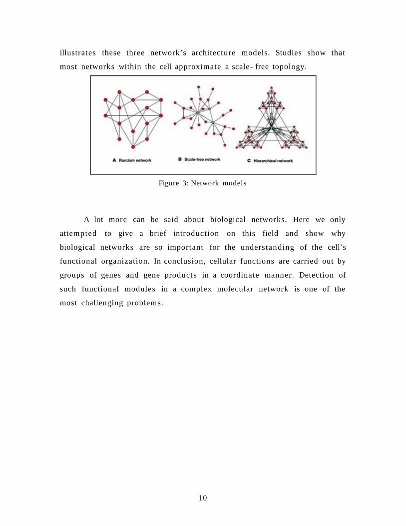
illustrates these three network’s architecture models. Studies show that
most networks within the cell approximate a scale- free topology.
Figure 3: Network models
A lot more can be said about biological networks. Here we only
attempted to give a brief introduction on this field and show why
biological networks are so important for the understanding of the cell’s
functional organization. In conclusion, cellular functions are carried out by
groups of genes and gene products in a coordinate manner. Detection of
such functional modules in a complex molecular network is one of the
most challenging problems.
10

3. Related work
The goal of this section is to compare Cellstorm with a set of
existing software systems that are widely used as visualization tools in
several biology fields. All the tools presented in this chapter work with
large data sets of genes and other genes’ related data, for example
networks data.
3.1. Cytoscape
Cytoscape is an open source Java- based software platform that
works on all major operating systems and that can be used for visualizing
networks of any type, as long as data are formatted in Simple Interaction
Format (SIF; three columns indicating interacting molecules and the type of
interaction).
Cytoscape can be extended through a plug- in architecture, allowing
rapid development of additional computational analyses and features.
Viewing and Filtering a Network
We start Cytoscape by loading the network data from a SIF file, or
the user can create the network data manually by using Cytoscape editing
tools. If the network has thousands of nodes, the user can filter the data
using measures of node and edge density which can help organize the
network into highly connected sub- networks.
11

Once the network data is fully loaded Cytoscape provides a wide
range of display layouts: layouts based on spring forces, layouts that try to
detect certain types of graph structure, annotation - based layouts, and
many others. Networks can be easily browsed, nodes and edges can be
selected, and their attributes examined. Nodes can also be searched for by
ID.
Combining Interaction and Expression Data
With Cytoscape the user can overlap expression information to
identify any patterns. Cytoscape offers easy ways to import expression
information where the key requirement is the use of the same
nomenclature system for interactions and expression. Once expression
data are linked to the nodes, the user has several choices about how to use
these data. Using a numeric filter, nodes above or below a threshold
expression value/ratio can be selected. Otherwise, nodes can be colored
one of several colors in a spectrum depending on user defined cutoffs.
Cellstorm does not offer the capability of importing expression
information other than the one already present and it only provides a
numeric filter for nodes with more genes or less genes than a threshold
value (Visibility threshold window).
Comparison with Cellstorm
Cellstorm is not as flexible as Cytoscape in terms of including
different display layouts. This is one of the powerful sides of Cytoscape.
Nevertheless the lack of flexibility allows Cellstorm to be less complex and
easier to use by any type of users. Cellstorm is a simple applet that can be
12

loaded in a few seconds and offers a clear user interface to visualize
networks.
Suppose that one wanted to analyze different networks selectively
within Cytoscape. It would be possible to create a node for each subcellular
component and to draw links between the nodes, but a front end program
would have to offer Cellstorm’s (i) zooming facility; (ii) import and export
facilities based on user selections; (iii) ability to dynamically select links;
Therefore, Cellstorm gives more insight than Cytoscape for the same
application.
The next figure shows a Sample Cytoscape Plugin for Interfacing
with cPath. The Cytoscape Expression Viewer plugin enables researchers to
visualize expression data on biological pathways. The plugin utilizes the
cPath web service API to retrieve pathway data, such as the Kit receptor
pathway from the Cancer Cell Map.
13
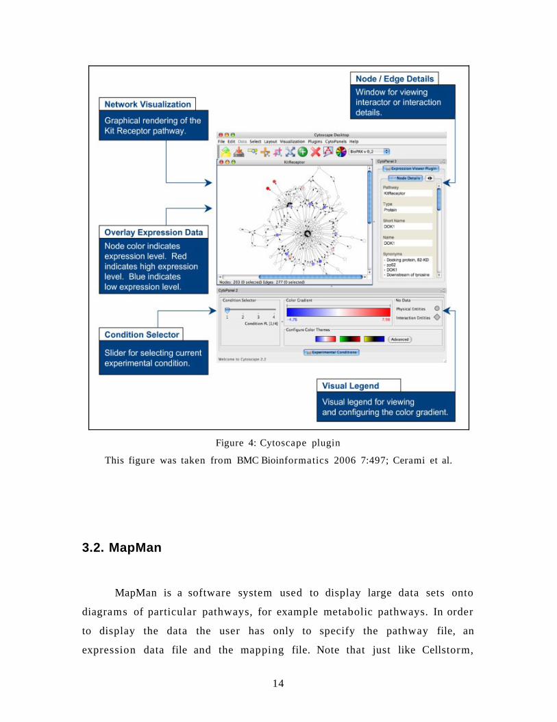
Figure 4: Cytoscape plugin
This figure was taken from BMC Bioinformatics 2006 7:497; Cerami et al.
3.2. MapMan
MapMan is a software system used to display large data sets onto
diagrams of particular pathways, for example metabolic pathways. In order
to display the data the user has only to specify the pathway file, an
expression data file and the mapping file. Note that just like Cellstorm,
14

Mapman is a general tool that avoids building on data - specific
assumptions.
In MapMan each pathway is arranged into hierarchical categories,
BINs and subBINs which are given locations within the diagram according
to the selected pathway. The expressed data is then assigned to one or
more of these BINs forming a MapMan diagram. A continuous color map
going from red to blue to designate the data expression value is used to
help find the locations with higher and lower levels of expressed data, for
example expressed genes.
The next image is a MapMan diagram of pathway level display of
genes involved in the TCA cycle, glyoxylate cycle, gluconeogenesis and
other organic acid transformations.
15

Figure 5:. This figure was taken from The Plant Journal(2004) 37, pag 927; Oliver
Thimm et al.
In addition to displaying pathway diagrams, MapMan also offers a
variety of tools to get information like for example gene names, expression
values, and other data properties and statistics.
Comparison with Cellstorm
The use of MapMan can be complementary to Cellstorm. While
Mapman displays entire paths and a relatively small number of genes
(scores at most) annotated to that pathway, Cellstorm is focused on single
links and can abstract a network in such a way as to show an arbitrary
number of links. MapMan is a very static application and doesn’t try to
offer the dynamic interaction that Cellstorm offers.
16

3.3. Pathway Studio
Pathway Studio is a software system for gene expression analysis
focusing on biological principles rather than on the selection of gene lists.
With Pathway Studio the user can import raw gene expression data files
and generate interaction maps to show possible regulation events and the
highly affected entities.
Pathway Studio offers a wide and diverse range of features going
from building and visualizing pathways, importing and analyzing gene and
protein lists, interpreting microarray gene expression data among others.
In this section we only present pathway visualization since this is the
feature that most relates with Cellstorm.
Pathway visualization
This Pathway Studio feature consists of a graphical user interface for
drawing, coloring, viewing, editing and annotating of pathway and
relationship maps. Very much like MapMan, the layout reveals pathway
organization. A very interesting layout is by cell localization. This layout
option automatically arranges entities by their localization in a cell. Other
layouts are also possible. Please see figure 6 for an example of cell layout.
Comparison with Cellstorm
While Pathway Studio looks at specific interactions, for example
sub- cellular interactions, Cellstorm with its zooming feature, is more
general allowing to look at interactions in different hierarchical levels. For
example, with Cellstorm we can look at biological networks between
different root cells, and going one level down, we can look at specific sub-
17

cellular interactions. We are not restricted to only one level on the
hierarchy. Cellstorm is much more dynamic than Pathway Studio and that
is a big advantage.
In terms of layout, Cellstorm may have less options; Cellstorm does
not present a range of different layouts and does not display components
using specific images or incorporating location information from
pathways. Nevertheless, Cellstorm offers other features that will be very
important for a user that is interested in visualizing networks and its
structure. In Pathway Studio the layout does not bring any information
about the expression values. While in Cellstorm we have highways with
different thickness representing the number of links and subcomponents
with different sizes representing the number of annotated genes. In
Pathway Studio we cannot get that information intuitively from the
displayed image.
The next image was taken from the Pathway Studio website and
illustrates the use of pathway using layout by cell localization.
18

Figure 6: Pathway layout by cell localization
3.4. Sungear
Sungear is a complementary application to Cellstorm.
Sungear enables rapid, visually interactive exploration of large sets
of genomic data. It allows browsing of gene sets by experiment
membership, gene annotation, and ontological term. Its intuitive interface
enables the user to quickly find the data sets that play a role in a function
of interest. The purpose of Sungear is to make otherwise complicated
queries quick and visually intuitive.
19

Figure 7: Example of the Sungear interface
This image was taken from Sungear’s paper ; C. Poultney et al.
Comparison with Cellstorm
Sungear is a very powerful tool but does not offer any feature to
visualize networks data. In fact we designed Cellstorm to fill exactly this
gap.. Therefore these tools are made to complement each other. With
Sungear the user can select the set of genes that he is interested in
analyzing. The user can then import this list into Cellstorm to visualize the
networks. Note that besides the network data that Cellstorm needs to get
as input file, Sungear and Cellstorm use just the same data import files.
20

4. Cellstorm Interface
Cellstorm is manly an interactive graphical tool that allows a very
rapid visualization of data. Therefore the user interface is a very important
aspect of this work. In this chapter we will describe the main features
covered by Cellstorm.
The most relevant property of Cellstorm is that display size and
quantity (number of genes expressed in a subcomponent or number of
links present in a network connection) are directly interconnected,
meaning that size is proportional to quantity.
21

4.1. Subcomponents
Cellstorm starts by receiving a list of genes selected externally,
either by the user, Sungear or other Virtual Plant applications. Once the
gene list is received, Cellstorm intersects the gene list and the genes
associated with each subcomponent. Each subcomponent will be bigger if
it has lots of genes from this intersection and smaller otherwise. This will
allow the user to intuitively see which subcomponent has more expressed
genes.
We illustrate this feature in figure 8. We can immediately say that
subcomponent “cell” (meaning in all subcellular components) is the one
with the higher number of genes (320 genes), followed by “organelle”,
“CCU”, “PC” and so on. For this example the gene list has a total of 442
genes (top right corner) and we are using the Gene Ontology hierarchy. If
the user is interested in knowing the exact number of genes associated
with each subcomponent, he only has to position the mouse on top of the
subcomponent and that number will be displayed as we can see for “cell”
subcomponent. To see the list explicitly the user may click on top of the
subcomponent and the list will be displayed. Please refer to Figure 5 to see
an example of this feature.
22

Figure 8: Graphical display of subcomponents of cellular_component
Figure 9: List of genes in “envelope”
The user has the options to Add, Remove or Intersect the displayed
genes to the user’s pre existing list of genes. When the application is
loaded for the first time, the user’s list is empty. In figure 8, bottom right
corner, we can see the number of genes in the user’s list and by clicking in
the link “My list” a pop up window will open with the actual list of genes,
23

please see figure 10 for an example.
As for the options, “Add”, will add the displayed genes that don’t
already exist in the user’s list, “Remove”, will remove the displayed genes
that exist in the user’s list and “Intersect”, will keep the genes that exist
both in the displayed list and the user’s list. OK, will close the window.
Figure 10: User’s gene list
In case an export_url was provided to Cellstorm through the query
string, then the button “Export” in the “My gene list” will be active and by
clicking on it the user has the ability to export its own list to that
export_url. In figure 10 we can see the “My gene list” window with the
Export button.
At any point in time, the user may select away subcomponents to
reduce clutter and to prune the gene list. Figure 11 shows an example
where this feature may be important to use due to the graphic complexity
originated by the high number of subcomponents present for “cytoplasm”.
24

Figure 11: Graphical display of subcomponents and networks of cytoplasm
If the user changes the visibility for example to 3 (see figure 13),
then the subcomponents with less than 3 genes will not be displayed.
Figure 12 shows the result of applying this new visibility threshold.
Figure 12: Graphical display of subcomponents and networks of cytoplasm with
25

threshold set to 3
By comparing figure 11 and figure 12, we can see the benefits of
changing the visibility threshold. Note that the total number of genes has
been reduced as well, in figure 11 we see that there are 188 genes in the
list, after changing the visibility threshold the list has been reduced to 182
genes.
Figure 13: Changing visibility threshold
To finalize this section, just a final remark about the subcomponent
position. When the subcomponents are displayed, Cellstorm chooses a
default position using a circular /oval distribution and avoiding overlaps as
much as possible. However, the user can always change the
subcomponents position by dragging and dropping.
4.2. Zooming
Before delving into the graphical display of networks we will explain
how zooming works for Cellstorm. As mentioned before, Cellstorm expects
to have some basic data like entities, hierarchical categories, a set
membership file and networks data. Using the hierarchical categories,
every view in Cellstorm has a main container /component (e.g.
cellular_Component) and sub- containers / s ubcomponents (e.g cell, CCU,
PC, envelope, ML, organelle). Once this hierarchical structure is defined,
zooming in and zooming out will allow to browse through all elements in
26

the structure. This will be exemplified in the following figures.
Zooming- In on a subcomponent will retrieve a new view level where
the subcomponent is now the new main component. If we look at the
hierarchical structure as a graph, zooming- In makes the subcomponent
the new parent. Zooming- Out works the other way around. The previous
main component will now be just one of the children in the new view level.
Zooming- In and Out will allow the user to graphically traverse the graph.
Zooming- Out will not be available if we are at the top level and Zooming-
In applies only if there are some edges to draw in the lower level.
As for the interface, there are two ways to zoom- In and zoom- Out.
The most simple and fast option is to use the mouse wheel exactly the
same way as in Google maps, roll- up to zoom - In and roll- down to zoom-
Out. The other option is to use a pop- down menu where the name of the
subcomponent to zoom- In or zoom- Out may be selected from a list. This
is shown in figure 14.
Figure 14: Zooming- In and Zooming- Out
The next two figures exemplify how zooming works. Figure 15,
shows the result of zooming- In on “cell”. Note that the current view
(parent) is now cell.
27

Figure 15: Zooming- In and Zooming- Out
Figure 16, shows the result of zooming- out. Note that the new
current view is now cellular - component.
Figure 16: Zooming- In and Zooming- Out
28

4.3. Networks and links
As already mentioned before, Cellstorm receives networks
information from a multi - network static file which will be provided by the
system or by the user. Once the subcomponents are displayed, the user is
then offered a menu of network types to choose from (figure 17), e.g.
metabolic, protein: protein, regulation and so on. Each network has a color
which will allow a very rapid visualization.
When a network type is selected, “highways” of various
thicknesses are drawn between the subcomponents. The highway size or
thickness, is proportional to the number of links that relate a gene in one
node to a gene in a second node (which could be the same). So thicker
means more links and thinner means fewer links.
For directed networks we have one way highways with appropriate
thickness and an arrow representing the network direction. We may also
have undirected networks, with no arrows, or bidirectional networks, with
an arrow in each side. Figures 18 and 19 illustrate the networks display.
For each view level the networks selection list (figure 17) may vary.
Only the networks with links will be displayed in this list for each view
level.
Also, the user has the option to hide or show self- loops. This may be
used to reduce graphic complexity. Another important aspect of the self-
loops is that by looking at a subcomponent’s self- loops the user can have
an idea of the networks that will be displayed when zooming- In on that
subcomponent.
29

Figure 17: Networks selection
The user selects only the networks that he or she is interested in
viewing. As mentioned before, if a network has no links then the network
checkbox is not displayed. Mousing over a network type will display the
number of links for that network.
30

Figure 18: Networks between subcomponents of cellular_component without self-
loops
Figure 19: Networks between subcomponents of cellular_component with self-
loops
In figure 18 we see that the thicker “highway” corresponds to the
blue network “Reaction” between “organelle” and “cell” meaning that this
network has the highest number of links (106 links /gene pairs), on the
other side, the red network, “Protein: protein” is the one with the lowest
number of links.
Also this figure shows the three different directional types of
networks: “Protein: protein” and “Reaction” are undirected networks,
“Reversible Reaction” is a bi- directed network and finally “Irreversible
Reaction (important)” is a directed network.
31

For directed networks, we may have a “highway” going from C1 to
C2 but none going from C2 to C1. In figure 18, this is the case for
“Irreversible Reaction (important)” between “CCU” and “cell” or between
“CCU” and “organelle”. If both “highways” are present one may be thicker
than the other. Again in figure 18 for “Irreversible Reaction(important)” we
have a “highway” with 32 links from “organelle” to “cell” and a “highway”
with 30 links from “cell” to “organelle”. Therefore the “highway” going
from “organelle” to “cell” is slightly thicker.
The user has a variety of mouse events that can be used to extract
more information from the networks. Mousing over a “highway” will
display the number of links /gene pairs. A mouse click opens a new window
with the gene pairs (figure 20).
Figure 20: Network gene pairs
32

The user has the options to Add, Remove or Intersect the displayed
genes to the user’s own list of genes the same way as for subcomponents.
5. Cellstorm design
A major design issue for Cellstorm concerned the choice between a
server - side language like Perl or Python or a client - side language like Java.
To get a more interactive application, and since all the data is loaded from
text files provided by the user, we decided to use Java.
Cellstorm consists of a Java applet that can be used directly on the
World Wide Web (internet). A Cellstorm application starts by reading a few
text files and loading the data in the corresponding data structures. Once
the loading process is complete the user can start using the application.
Achieving good performance in Cellstorm was an interesting
challenge. As an interactive application we wanted Cellstorm to handle
(load and retrieve) data as fast as possible. By using Java’s class Hash
Tables and Hash Sets to create Cellstorm’s data structures we were able to
achieve a good performance level for loading and retrieval.
A Cellstorm application is divided into two main windows. The
display window on the left and the control panel window on the right. An
action done in the control panel will always take effect on the display
section. In more detail, inside the control panel we have three sub-
windows. The networks window, the zooming window and the visibility
33

threshold window. Any of these windows offer a set of options that can be
selected by the user. See figure 21.
Figure 21: Cellstorm windows
In the next two sections we will explain in more detail Cellstorm’s
data and modules.
5.1 Data
As mentioned before, Cellstorm expects to have some basic data
like: entities, hierarchical categories, a set membership file and networks
data. For Arabidopsis, these are genes, GO (gene ontology) terms, the gene
34

list /set membership input file and the multi - networks file. The data is
provided to Cellstorm as a set of text files.
5.1.1 Gene Ontology
GO terms used by Cellstorm (by default) are provided by the Gene
Ontology project which offers consistent description of gene and gene
products attributes in any organism.
The GO project has developed three structured ontologies that
describe gene products in terms of their associated biological processes,
cellular components and molecular functions in a species - independent
manner.
The ontologies are structured as directed acyclic graphs (DAGs)
providing an hierarchical structure used by Cellstorm to create different
view levels. Note that each child in these structures may have more than
one parent.
GO terms have a unique numerical identifier of the form
GO:nnnnnnn , and a term name, e.g. cell . Each term is also assigned to one
of the three ontologies, molecular function, cellular component or
biological process. A gene product might be associated with or located in
one or more cellular components.
Cellstorm can use any of the three ontologies, however many
Cellstorm applications will use the cellular component ontology which
describes locations at the levels of subcellular structures and
macromolecular complexes. Generally, a gene product is located in or is a
subcomponent of a particular cellular component.
35

In order to maintain a hierarchical structure, each GO term has a
path to the root node (cellular component) which passes solely through
is_a relationships which means that there are is_a parent terms by at least
one path all the way to cellular component.
5.1.2 Files and formatting
Cellstorm may be used with different species. The user will have to
provide Cellstorm with the species name, gene annotation file, GO term
annotation file, GO term hierarchy file, GO term / gene correspondence
file, network file and network configuration file.
The file formatting is general for all the species. In this section we
will illustrate the files format by using Arabidopsis files.
• Species name: Arabidopsis
• The gene annotation file contains pairs (gene ID | gene description):
At3g26090 | expressed protein
At5g65080 | MADS- box family protein
…
• The GO term annotation file contains pairs (GO ID | GO description):
GO:0000001 | mitochondrion inheritance
GO:0000002 | mitochondrial genome maintenance
…
• The GO term hierarchy file contains rows like
(parent GO ID | list_of_child_go_ids)
GO:0000018 | GO:0045910 GO:0045911 GO:0000337 GO:0000019
GO:0000087 | GO:0007072 GO:0000281 GO:0007067
36

GO:0000023 | GO:0000024 GO:0000025
…
• The GO term / gene correspondence file contains rows like
(GO ID | z- score | gene1list - of_gene_ids)
GO:0000002 | 1.1503067484662577E- 4 | At5g46400 At1g10270
GO:0000003 | 0.005138036809815951 | At3g20740
…
Note that for the scope of this project z- score values are not used;
• The network file contains rows like
(Origin /tab Network name /tab Destination)
At5g59710 interolog:pp At4g00660
At3g56150 interact At4g14110
At1g77070 regulog:pp At5g24760
1,2- Diacyl- sn- glycerol Irc At1g02660
10- Formyltetrahydrofolate Irc At4g17360
…
The network file follows the Simple Interaction Format, SIF, three
columns indicating interacting molecules (origin and destination) and
the interaction type;
• The network configuration file contains rows like
(network pretty name | network name | network type | network
color)
Interaction | interact | none | 153,102,51
Predicted protein:protein | interolog:pp | none | 153,0,204
Irreversible Reaction (important) | Irc | directional | 255,204,0
Positive Regulation | activate | directional | 255,102,0
…
• Gene List contains a list of genes
At1g01050
37

At1g01450
At1g01460
At1g01510
At1g01560
…
5.2 Modules
In this section we will describe each of the eight classes maintained
in Cellstorm.
• Class Gene
Data: id, name, location, gene_is_a
The gene location is the GO terms where the gene is annotated. The
gene_is_a is the list of GO terms to which the gene is annotated and its
ancestors in the cellular component ontology;
Methods: setName, setLocation, setGene_is_a, getId,
getName,getGene_is_a
• Class Goterm
Data: id, name, parent, children
Both parent and children are taken from the gene ontology
hierarchy;
Methods: setId, setName, setChildren, setParent, getId, getName,
getChildren, getParent, copy, clean, print
38

• Class Network
Data: nodeA, nodeB, label, name, direction, type, netColor
Methods: getName, getPrettyName, getType, getOrigin,
getDestination, getDirection, getColor
• Class Shape is abstract
Methods: getX, getY, getWidth, getHeight, getId, getName
• Class SubComponent extends Shape
Data: id, name, x, y, width, height, color, shape, geneList, geneCount
Methods: setSize, setCoordinates, adjustCoordinates, setDragged,
setColor, setShape, addGeneList, contains, getNumGenes, getName,
getX, getY, getWidth, getHeight, setBounds, getId, getGeneList,
getGeneSet, draw
• Class Link
Data: color, thickness, origin, destination, type, name, weight,
genePairs, divFactor, curve, netWidth
Methods: setColor, equal, isPair, addThickness, getThickness,
addDivisionFactor, addGenePair, getListSize, getGenePairs,
getGeneSet, getName, getOriginName, getDestinationName,
getDirection, drawArrowFormat, contains, drawCurvedArrows, draw,
• Class Cellstorm extends JApplet implements Runnable
This is the main module where all graphical components that
compose Cellstorm interface are created. It’s also in this module
that all the data structures are defined and the data is loaded from the
text files
39

• Class Display extends JPanel implements MouseListener,
MouseMotionListener, MouseWheelListener; This is a nested class
that represents the drawing surface of the applet
Data: width, height, graphic2D
5.3 Program structure
Cellstorm starts with two different threads. One thread creates the
Graphical User Interface; the other thread will take care of more time
consuming tasks as reading and loading data. Most often the GUI is
displayed even before the data has been processed.
The GUI creation thread starts by creating the component for the
drawing area using the Display class. Then it creates the main control
panel followed by the network panel, zooming panel and threshold options
panel. All these three panels are added to the control panel. Finally, the
drawing area and control panel are both added to the Applet.
The second thread starts by reading gene and go term data and
filling the correspondent data structures. This thread reads the data by the
following order: gene list, gene annotation, go to gene, go term annotation,
go hierarchy, network configuration and networks. Once all the data is
processed then the zooming area, visibility threshold and network area are
created and filled with data.
In the next chapter (Cellstorm implementation) we will describe in
more detail how the data is loaded into Cellstorm data structures.
40

6. Cellstorm implementation
In this section we will describe the major Cellstorm data structures,
some graphical components and the most important algorithms.
6.1 Cellstorm major data structures
• From the gene list file and gene annotation file Cellstorm creates a
geneMap that consists of pairs (Gene_ID, Gene). The map size
41

matches the gene list size however if a given gene does not exist in
the gene annotation file than it will be discarded.
Map<String, Gene> geneMap = new Hashtable<String, Gene>();
• From the go term annotation file Cellstorm creates a goMap that
consists of pairs (Go_ID, Goterm). The map size matches the file
size.
Map<String, Goterm> goMap = new Hashtable<String, Goterm>();
• From the network configuration file Cellstorm creates several
different network maps that will contains the different network
properties.
Map<String, String> networkMapName = new Hashtable<String, String>();
Map<String, String> networkMapType = new Hashtable<String, String>();
Map<String, String> networkMapColor = new Hashtable<String, String>();
• From the networks data file Cellstorm creates a networks set that
consists of entries that have at least one node belonging to geneMap.
So, any entry in the network file that does not have an origin or a
destination from the gene list will be discarded. Since the network
file is usually very big, this implementation strategy is important to
reduce the number of networks to be loaded in Cellstorm and
therefore to reduce the loading and processing time. It also reduces
the visual clutter.
42

Set<Network> networks = new HashSet<Network>();
• Other important data structures related to Gene and Goterm data
// Selected Genes in My List
Set<String> selectedGenes = new HashSet<String>();
// The top component in the hierarchy (Applet parameter)
String TopComponent;
// zoom in pushes terms to the history stack
// zoom out pops terms from the history stack
Stack<Goterm> history = new Stack<Goterm>();
• Other important data structures related to networks data
// set of all network types
Set<String> networksType = new HashSet<String>();
// types that have been selected by the user
Set<String> selectedNetworks = new HashSet<String>();
// types that are active for each zoom level
Set<String> activeNetworks = new HashSet<String>();
// network's pretty name
Set<String> prettyName = new HashSet<String>();
// network weigths to be used to draw the curved highways
Map<String, Double> networkWeight = new Hashtable<String, Double>();
// Apply associative rule: gene-other + other-gene => gene-gene
Map<String, Set<Network>> origin_map = new Hashtable<String,
Set<Network>>();
43

Map<String, Set<Network>> destination_map = new Hashtable<String,
Set<Network>>();
6.2 Cellstorm major graphical components
• Main window
// Applet width and height
int w,h;
JPanel canvasPanel;
JPanel controlPanel;
JScrollPane controlPanelScroll;
• Canvas Panel
// list of subcomponents to be displayed in the canvas
Vector<SubComponent> shapes = new Vector<SubComponent>();
// list of links between subcomponents
Set<Link> links = new HashSet<Link>();
• Control Panel
JPanel networkPanel;
JPanel zoomPanel;
JPanel thresholdPanel;
• Network Panel
Map<String, JCheckBox> networkMap = new Hashtable<String, JCheckBox>();
• Zoom Panel
44

JButton zoomIn, zoomOut;
ImageIcon ImageZoomIn = createImageIcon("zoom_in.jpg","Zoom_IN");
ImageIcon ImageZoomOut = createImageIcon("zoom_out.jpg","Zoom_OUT");
JLabel currentComponent;
JComboBox zoomInChoice, zoomOutChoice;
ComboBoxModel modelChildren, modelParent;
• Threshold Panel
JButton changeThreshold;
JComboBox thresholdChoice;
JLabel thresholdLabel;
6.3 Cellstorm Major Algorithms
6.3.1. Subcomponent placement algorithm
For each view level Cellstorm has a variable number of
subcomponents that must be displayed in the canvas area. Cellstorm
displays the group of subcomponents in an ellipse - shaped diagram. Next
we present the algorithm outline.
- Ellipse center:
int centerX = 10 + (width-20)/2;
int centerY = 40 + (height-80)/2;
- Number of subcomponents:
int numSubComp = shapes.size();
- Ellipse semi major axis and semi minor axis:
45

int radiumX = 3*(width-20)/7;
int radiumY = 3*(height-80)/7;
- Distance between subcomponents:
double theta;
if (numSubComp > 2)
{ theta = 2*Math.PI/numSubComp; }
else
{ theta = 2*Math.PI/3; }
- Subcomponent location. Coordinates location for subcomponent top left
corner:
double x = radiumX * Math.cos(i*theta);
double y = radiumY * Math.sin(i*theta);
int xCoord = centerX+(int)x-(maxSizeW/2);
int yCoord = centerY+(int)y-(maxSizeH/2);
shapes.get(i).setCoordinates(xCoord,yCoord);
- Subcomponents maximum size. This is the size of the subcomponent
with more genes:
int maxSizeH = Math.min( 80, (int)(radiumY * Math.sin(theta) - 20.0));
int maxSizeW = maxSizeH;
if (width - height > 0)
{ maxSizeW = maxSizeW + (width-height)/4; }
- Subcomponent size using linear interpolation. Size is proportional to
quantity of genes:
46
if (maxGenes != 0)
{ width = (width/2 + ((geneList.size()/maxGenes) * (width/2)));
height = (height/2 + ((geneList.size()/maxGenes) * (height/2)));
}
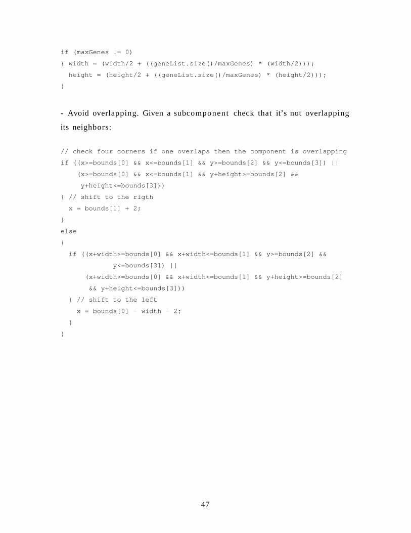
- Avoid overlapping. Given a subcomponent check that it’s not overlapping
its neighbors:
// check four corners if one overlaps then the component is overlapping
if ((x>=bounds[0] && x<=bounds[1] && y>=bounds[2] && y<=bounds[3]) ||
(x>=bounds[0] && x<=bounds[1] && y+height>=bounds[2] &&
y+height<=bounds[3]))
{ // shift to the rigth
x = bounds[1] + 2;
}
else
{
if ((x+width>=bounds[0] && x+width<=bounds[1] && y>=bounds[2] &&
y<=bounds[3]) ||
(x+width>=bounds[0] && x+width<=bounds[1] && y+height>=bounds[2]
&& y+height<=bounds[3]))
{ // shift to the left
x = bounds[0] - width - 2;
}
}
47

6.3.2. Drawing highways – thickness and quadratic curves
Given two subcomponents, Cellstorm displays the networks between
them using quadratic curves whose thickness is proportional to the
number of gene pairs retrieved for each network type. Depending on the
type of network, the end points of the quadratic curve may or may not be
arrows. Directed – one arrow representing the network direction;
Undirected – no arrows; Bi- directed – two arrows one in each side. Next we
present the algorithm outline.
- Assign a different weight to each network type. Between two
subcomponents we may have several different network types. In order to
avoid the overlapping of each network must have a specific weight that will
serve as a measure to get the quadratic curve control points:
int totalNet = prettyName.size();
int i = 0;
Iterator it_prettyName = prettyName.iterator();
while(it_prettyName.hasNext())
{ String Net_prettyName = (String)it_prettyName.next();
networkWeight.put(Net_prettyName,(i*1.0/(totalNet*1.0 - 1)));
i++;
};
- Get division factor for directed networks. Directed networks need to have
two different weights, one for each direction. We use the division factor to
split one weight into two different weights:
divisionFactor = 1.0/(totalNet*1.0 - 1);
48

- Get maximum number of gene- pairs to be used for thickness:
Iterator it_link = links.iterator();
while(it_link.hasNext())
{
Link link = (Link)it_link.next();
maxGenePairs = Math.max(link.getListSize(),maxGenePairs);
}
- Get network width (known as thickness):
netWidth = (maxSize/5 + ((maxSize-maxSize/5)*1.0/maxGenePairs)
*genePairs.size())/(1.5);
- Get origin and destination center points:
// Origin center point
double Ocx = origin.getX() + origin.getWidth()/2;
double Ocy = origin.getY() + origin.getHeight()/2;
// Destination center point
double Dcx = destination.getX() + destination.getWidth()/2;
double Dcy = destination.getY() + destination.getHeight()/2;
- Get slope of line that connects Origin and Destination center points:
t = ((Ocy-Dcy)*1.0/(Ocx-Dcx));
- Find bisector of previous line (connects Origin and Destination center
points). The control points will be always on top of bisector line. The next
figure illustrates how we get the bisector line and helps to follow the code.
49

Figure 22: Algorithm illustration
double h = Math.sqrt((Ocx-Dcx)*(Ocx-Dcx) + (Ocy-Dcy)*(Ocy-Dcy));
double l = h/Math.sqrt(2);
double alfa = Math.asin(Math.min(Math.abs(Ocx-Dcx),Math.abs(Ocy-
Dcy))/h);
double beta = Math.acos(Math.min(Math.abs(Ocx-Dcx),Math.abs(Ocy-
Dcy))/h);
double gamma;
if (Math.abs(t)<1)
{ gamma = Math.PI/2 - Math.min(alfa,beta) - Math.PI/4; }
else
{ gamma = beta - Math.PI/4; }
double a = l*Math.sin(gamma);
double b = l*Math.cos(gamma);
50
Orig
Dest
a
b
Line connecting Orig to Dest
Bisector Line
Angle alpha
Angle gamma
Angle beta
Oy - Dy

- Get bisector start and end points (x1,y1) (x2,y2):
double x1,y1,x2,y2;
if (t>0)
{ if (Math.abs(t) < 1)
{ x1 = Math.min(Ocx,Dcx) + a;
y1 = Math.min(Ocy,Dcy) + b;
x2 = Math.max(Ocx,Dcx) - a;
y2 = Math.max(Ocy,Dcy) - b;
}
else
{ x1 = Math.max(Ocx,Dcx) - b;
y1 = Math.max(Ocy,Dcy) - a;
x2 = Math.min(Ocx,Dcx) + b;
y2 = Math.min(Ocy,Dcy) + a;
}
}
else
{ if (Math.abs(t) < 1)
{ x1 = Math.min(Ocx,Dcx) + b;
y1 = Math.max(Ocy,Dcy) + a;
x2 = Math.min(Ocx,Dcx) + a;
y2 = Math.max(Ocy,Dcy) - b;
}
else
{ x1 = Math.max(Ocx,Dcx) + a;
y1 = Math.min(Ocy,Dcy) + b;
x2 = Math.min(Ocx,Dcx) - a;
y2 = Math.max(Ocy,Dcy) - b;
}
}
51

- Get quadratic curve (link) control points:
double m = (y2-y1)/(x2-x1);
double c = y1 - m*x1;
double ctrlx, ctrly;
if (m!=0 && m!=Double.POSITIVE_INFINITY && m!=Double.NEGATIVE_INFINITY)
{ ctrly = Math.min(y1,y2) + Math.abs(y1-y2)*weight;
ctrlx = (ctrly - c)/m;
}
else
{
if (m==0)
{ ctrlx = Math.min(x1,x2) + Math.abs(x1-x2)*weight;
ctrly = y1;
}
else
{ ctrlx = x1;
ctrly = Math.min(y1,y2) + Math.abs(y1-y2)*weight;
}
}
- Get curve’s origin and destination. If the subcomponents are very close
then these points will be the center points of the subcomponents,
otherwise these points will be the intersection points between the
quadratic curve and the subcomponent shape. Next we show how to get
these values:
// - find intersection point for origin SubComponent
if (Ocx-ctrlx !=0)
{ // intersects with vertical left ?
x = Ocx - origin.getWidth()/2 - netWidth;
y = m1*x + b1;
if (y>=Ocy-origin.getHeight()/2-netWidth &&
y<=Ocy+origin.getHeight()/2+netWidth && y>=Math.min(Ocy,ctrly) &&
y<=Math.max(Ocy,ctrly))
{ Ox = x; Oy = y; }
52

// intects with vertical right ?
x = Ocx + origin.getWidth()/2 + netWidth;
y = m1*x + b1;
if (y>=Ocy-origin.getHeight()/2-netWidth &&
y<=Ocy+origin.getHeight()/2+netWidth && y>=Math.min(Ocy,ctrly) &&
y<=Math.max(Ocy,ctrly))
{ Ox = x; Oy = y;}
}
if (Ocy-ctrly !=0)
{ // intects with horizontal top ?
y = Ocy - origin.getHeight()/2 - netWidth;
x = (y-b1)/m1;
if (x>=Ocx-origin.getWidth()/2-netWidth &&
x<=Ocx+origin.getWidth()/2+netWidth && y>=Math.min(Ocy,ctrly) &&
y<=Math.max(Ocy,ctrly))
{ Ox = x; Oy = y;}
// intects with horizontal bottom ?
y = Ocy + origin.getHeight()/2 + netWidth;
x = (y-b1)/m1;
if (x>=Ocx-origin.getWidth()/2-netWidth &&
x<=Ocx+origin.getWidth()/2+netWidth && y>=Math.min(Ocy,ctrly) &&
y<=Math.max(Ocy,ctrly))
{ Ox = x; Oy = y;}
}
// - find intersection point for destination SubComponent
if (Dcx-ctrlx !=0)
{ // intersects with vertical left ?
x = Dcx - destination.getWidth()/2 - netWidth;
y = m2*x + b2;
if (y>=Dcy-destination.getHeight()/2-netWidth &&
y<=Dcy+destination.getHeight()/2+netWidth &&
y>=Math.min(Dcy,ctrly) && y<=Math.max(Dcy,ctrly))
{ Dx = x; Dy = y;}
53

// intects with vertical right ?
x = Dcx + destination.getWidth()/2 + netWidth;
y = m2*x + b2;
if (y>=Dcy-destination.getHeight()/2-netWidth &&
y<=Dcy+destination.getHeight()/2+netWidth &&
y>=Math.min(Dcy,ctrly) && y<=Math.max(Dcy,ctrly))
{ Dx = x; Dy = y;}
}
if (Dcy-ctrly !=0)
{ // intects with horizontal top ?
y = Dcy - destination.getHeight()/2 - netWidth;
x = (y-b2)/m2;
if (x>=Dcx-destination.getWidth()/2-netWidth &&
x<=Dcx+destination.getWidth()/2+netWidth &&
y>=Math.min(Dcy,ctrly) && y<=Math.max(Dcy,ctrly))
{ Dx = x; Dy = y;}
// intects with horizontal bottom ?
y = Dcy + destination.getHeight()/2 + netWidth;
x = (y-b2)/m2;
if (x>=Dcx-destination.getWidth()/2-netWidth &&
x<=Dcx+destination.getWidth()/2+netWidth &&
y>=Math.min(Dcy,ctrly) && y<=Math.max(Dcy,ctrly))
{ Dx = x; Dy = y;}
}
}
- Draw quadratic curve:
g.setStroke( newBasicStroke((float)netWidth,BasicStroke.CAP_SQUARE,
BasicStroke.JOIN_ROUND));
curve = new QuadCurve2D.Double((double)Ox, (double)Oy, (double)ctrlx,
(double)ctrly, (double)Dx, (double)Dy);
drawCurvedArrows(g,(float)Ox,(float)Oy,(float)Dx,(float)Dy,(float)(netW
54

idth),(float)ctrlx,(float)ctrly);
7. Cellstorm Integration
Cellstorm is part of a bigger project called VirtualPlant. VirtualPlant
integrates genomic data and provides visualization and analysis tools for
rapid and efficient exploration of genomic data. Cellstorm belongs to that
group of tools.
Cellstorm is located in the VirtualPlant web server
/var /www/h tml /cellstorm and is launched from the VirtualPlant export
page by selecting Cellstorm from the pop- down list together with one or
several group of genes to analyze. Figures 23 and 24 show Cellstorm being
selected and launched from VirtualPlant page.
Figure 23: Cellstorm windows
55

Figure 24: Cellstorm windows
From the selected group of genes VP makes a file and sends its URL
to Cellstorm in the query string as the “data_url”. VP also sends a few more
parameters that will be used by Cellstorm to send back information to VP.
The most important of these is the URL where VP expects the form
submission to add new group: “export_url”. The data files urls can also be
send in the query string using specific parameters. The following is a
typical query string passed from VirtualPlant to Cellstorm:
http: / /vir tualplant.bio.nyu.edu /cellstorm /cellStorm1.html?
species=arabidopsis&
data_url= http: / /virtualplant.bio.nyu.edu /virtualplant / t emp / t em p5117612
2.sun &
export_url= http: / /vir tualplant - prod.bio.nyu.edu /cgi - bin/virtualplant.cgi &
56

export_cmd=addGroups&
export_action=session&
export_session_id=cc1f26aa8040f837f772dfe18bc24ffe
8. Use cases
In this section we will present two different test cases. The first case
shows Cellstorm being applied in a biological context. In the second case
Cellstorm is applied in a non- biological context. The second test case is
useful to demonstrate Cellstorm data independence.
8.1 Biological case study
We gratefully thank Miriam Gifford and Ken Birnbaum for supplying
the data for this test case.
In this case study we use Cellstorm to visualize network connections
between five different cell types within the root: Lateral Root Cap (LRC),
Epidermis&Cortex (EpiCor), Endodermis&Pericycle (EndoPeri), Pericycle
(Peri), Stele (Stele).
For each of these cell types we have the group of genes that are
nitrogen induced and nitrogen depressed. We have about 6,000 genes in
total. Note that genes can be nitrogen induced or depressed in more than
one cell type.
The data was grouped as nitrogen induced and nitrogen depressed.
For each of these groups we run Cellstorm for all genes and for cell
specific genes only.
57

In this case study the entities are Arabidopsis genes. The
hierarchical categories are: Root, LCR, EpiCor, EndoPeri, Peri and Stele
where the Root is the parent and all the other categories are Root’s
children. The membership is the nitrogen depressed / induced genes for
each cell type and finally the networks are the biological networks. The top
component in this case is the “Root”. Next we present some images from
this Cellstorm application, one per each different data group.
• Nitrogen induced:
Figure 25: Nitrogen induced using all genes
58

Figure 26: Nitrogen induced using cell specific genes only
• Nitrogen depressed:
Figure 27: Nitrogen depressed using all genes
59

Figure 28: Nitrogen depressed using cell specific genes only
8.2. Non- Biological case study
In this case study we use Cellstorm to show flight connections
between airports in different continents, countries and cities. The data for
this case study was built manually and does not attempt to represent a
complete set of flight connections.
Cellstorm expects entities, hierarchical categories, membership and
networks. In this case study the entities are airports, the hierarchical
categories are physical locations for example world, continents, countries,
states / regions, cities, the membership is where each airport is located and
finally the networks are the flight connections between different airports.
The top component in this case is the “World”.
Next we show several figures obtained from this case study. Figure
29 shows the top level view where the subcomponents are the 6
continents. Not surprisingly between continents we have more connections
60

for longer flights than for shorter flights.
Figure 29: Top level with flight connection
By zooming In on Europe we get the next figure that shows the flight
connections between some European countries. In this case, as we were
expecting, the longer flights disappeared and we only have connections for
shorter flights.
61

Figure 30: Zoom in to Europe
Next figure shows the airport locations for United Kingdom. We
obtain this figure by mouse clicking on top of the subcomponent “UK”.
Figure 31: Airport locations for United Kingdom
By mouse clicking in a link we obtain the list of connections between
two locations. Next figure shows the connections “between 2 and 3 hours”
from Portugal and United Kingdom.
62

Figure 32: Flight connections between Portugal and UK
9. Conclusion and Future Work
Cellstorm is a software system that allows a rapid visualization of
63

genes and subcellular networks. Given a set of genes, expression levels,
structural hierarchy and network’s data, Cellstorm displays the networks
at any level of the hierarchy and provides a set of user options such as
zooming, network selection and list filtering. In the graphical display the
most important property is that size is always proportional to quantity, for
example number of genes expressed in a subcomponent or number of
links present in a network connection.
Cellstorm is a generic tool that avoids building in data- specific
assumptions. Although it is targeted to be used in a biological context
Cellstorm can be applied in many other contexts as has been shown in
section 8.
Cellstorm was tested by some biology researchers and proved to be
a helpful tool to visualize networks in large datasets. Based on user
comments a variety of features may be added in the future to Cellstorm.
Here is a list of some suggestions:
• Connect Cellstorm directly from Sungear;
• Make the history (showed at the bottom of the display section)
interactive where clicking in a subcomponent name turns that
subcomponent to the present View level;
• Allow to view networks between genes /entities; The user would be
able to toggle between: display networks between subcomponents
and display networks between genes;
• Allow to create more than one list of genes and provide a more
flexible interface to add, remove and intersect list of genes;
64

10. References
[1] Albert - László Barabási & Zoltán N. Oltvai. Network Biology:
Understanding the cell’s functional Organization.
www.nature.com/ reviews /genetics
[2] George W. Bell and Fran Lewitter. DNA Microarrays, Part B, Visualizing
Networks.
[3] Paul Shannon, Andrew Markiel, Owen Ozier, Nitin S. Baliga, Jonathan T.
Wang, Daniel Ramage, Nada Amin, Benno Schwikowski and Trey Ideker.
Cytoscape: A Software Environment for Integrated Models of Biomolecular
Interaction Networks. Genome Res.2003 13: 2498- 2504.
[4] Oliver Thimm et al. MapMan: A user - driven tool to display genomics
data sets onto diagrams of metabolic pathways and other biological
processes. The Plant Journal (2004) 37, 914- 939.
[5] C. Poultney et al. Sungear: Interactive visualization and functional
analysis of genomic datasets. Bioinformatics Advance Access published
October 2,2006.
[6] The Gene Ontology project. www.geneontology.org
[7] Virtual Plant. http: / /vir tualplant - prod.bio.nyu.edu /cgi -
bin/virtualplant.cgi
[8] Pathway Studio. http: / /www.ariadnegenomics.com/p roducts / pa thway-
studio /
[9] James D. Tisdall. Perl Programming for Bioinformatics. Mastering Perl
65

for Bioinformatics
[10] Java documentation. http: / / j ava.sun.com /j2se /1.4.2 /docs /
66