Importance Sampling for Online Planningunder Uncertainty

Yuanfu Luo, Haoyu Bai, David Hsu, and Wee Sun Lee

National University of Singapore, Singapore 117417, Singapore

APPEARED IN

Proc. Int. Workshop on the Algorithmic Foundations of Robotics (WAFR), 2016

Abstract. The partially observable Markov decision process (POMDP) providesa principled general framework for robot planning under uncertainty. Leverag-ing the idea of Monte Carlo sampling, recent POMDP planning algorithms havescaled up to various challenging robotic tasks, including, e.g., real-time onlineplanning for autonomous vehicles. To further improve online planning perfor-mance, this paper presents IS-DESPOT, which introduces importance samplingto DESPOT, a state-of-the-art sampling-based POMDP algorithm for planningunder uncertainty. Importance sampling improves the planning performance whenthere are critical, but rare events, which are difficult to sample. We prove thatIS-DESPOT retains the theoretical guarantee of DESPOT. We present a generalmethod for learning the importance sampling distribution and demonstrate empir-ically that importance sampling significantly improves the performance of onlinePOMDP planning for suitable tasks.

1 Introduction

Uncertainty in robot control and sensing presents significant barriers to reliable robotoperation. The partially observable Markov decision process (POMDP) provides a prin-cipled general framework for robot decision making and planning under uncertainty [20].While POMDP planning is computationally intractable in the worst case, approximatePOMDP planning algorithms have scaled up to a wide variety of challenging tasksin robotics and beyond, e.g., autonomous driving [1], grasping [8], manipulation [13],disaster rescue management [25], and intelligent tutoring systems [4]. Many of these re-cent advances leverage probabilistic sampling for computational efficiency. This workinvestigates efficient sampling distributions for planning under uncertainty under thePOMDP framework.

A general idea for planning under uncertainty is to sample a finite set of “scenarios”that capture uncertainty approximately and compute an optimal or near-optimal planunder these sampled scenarios on the average. Theoretical analysis reveals that a smallsampled set guarantees near-optimal online planning, provided there exists an optimalplan with a compact representation [22]. In practice, the sampling distribution may havesignificant effect on the planning performance. Consider a de-mining robot navigatingin a mine field. Hitting a mine may have low probability, but severe consequence. Fail-ing to sample these rare, but critical events often results in sub-optimal plans.

Importance sampling [10] provides a well-established tool to address this challenge.We have developed IS-DESPOT, which applies importance sampling to DESPOT [22],a state-of-the-art sampling-based online POMDP algorithm (Section 3). The idea isto sample probabilistic events according to their “importance” instead of their naturalprobability of occurrence and then reweight the samples when computing the plan. We

prove that IS-DESPOT retains the theoretical guarantee of DESPOT. We also presenta general method for learning the importance sampling distribution (Section 4). Fi-nally, we present experimental results showing that importance sampling significantlyimproves the performance of online POMDP planning for suitable tasks (Section 5).

2 Background

2.1 POMDP Preliminaries

A POMDP models an agent acting in a partially observable stochastic environment. It isdefined formally as a tuple (S,A,Z, T,O,R, b0), where S,A and Z are the state space,the action space, and the observation space, respectively. The function T (s, a, s′) =p(s′|s, a) defines the probabilistic state transition from s ∈ S to s′ ∈ S, when the agenttakes an action a ∈ A. It can model imperfect robot control and environment changes.The function O(s, a, z) = p(z|s, a) defines a probabilistic observation model, whichcan capture robot sensor noise. The function R(s, a) defines a real-valued reward forthe agent when it takes action a ∈ A in state s ∈ S.

Because of imperfect sensing, the agent’s state is not known exactly. Instead, theagent maintains a belief, which is a probability distribution over S. The agent startswith an initial belief b0. At time t, it infers a new belief, according to Bayes’ rule, byincorporating information from the action at taken and the observation zt received:

bt(s′) = τ(bt−1, at, zt) = ηO(s′, at, zt)

∑s∈S

T (s, at, s′)bt−1(s), (1)

where η is a normalizing constant.A POMDP policy maps a belief to an action. The goal of POMDP planning is to

choose a policy π that maximizes its value, i.e., the expected total discounted reward,with initial belief b0:

Vπ(b0) = E( ∞∑t=0

γtR(st, at+1)∣∣∣ b0, π) (2)

where st is the state at time t, at+1 = π(bt) is the action taken at time t to reachst+1, and γ ∈ (0, 1) is a discount factor. The expectation is taken over the sequence ofuncertain state transitions and observations over time.

A key idea in POMDP planning is the belief tree (Fig. 1a). Each node of a belief treecorresponds to a belief b. At each node, the tree branches on every action a ∈ A andevery observation z ∈ Z. If a node b has a child node b′, then b′ = τ(b, a, z). To findan optimal plan, one way is to traverse the tree from the bottom up and and compute anoptimal action recursively at each node using the Bellman’s equation:

V ∗(b) = maxa∈A

{∑s∈S

b(s)R(s, a) + γ∑z∈Z

p(z|b, a)V ∗(τ(b, a, z)

)}. (3)

2.2 Importance Sampling

We want to calculate the expectation µ = E(f(s)

)=∫f(s)p(s) ds for a random

variable s distributed according to p, but the function f(s) is not integrable. One idea isto estimate µ by Monte Carlo sampling: µ̂ = (1/n)

∑ni=1 f(si), where si ∼ p for all

samples si, i = 1, 2, . . . , n. The estimator µ̂ is unbiased, with variance Var(µ̂) = σ2/n,where σ2 =

∫(f(s)− µ)2p(s) ds.

Importance sampling reduces the variance of the estimator by carefully choosing animportance distribution q for sampling instead of using p directly:

µ̂UIS =1

n

n∑i=1

f(si)p(si)

q(si)=

1

n

n∑i=1

f(si)w(si), si ∼ q, (4)

where w(si) = p(si)/q(si) is defined as the importance weight of the sample siand q(s) 6= 0 whenever f(s)p(s) 6= 0. The estimator µ̂UIS is also unbiased, withvariance Var(µ̂) = σ2/n, where σ2 =

∫( f(s)p(s)q(s) − µ)2q(s) ds. Clearly the choice

of q affects the estimator’s variance. The optimal importance distribution q∗(s) =|f(s)| p(s)

/Ep(|f(s)|

)gives the lowest variance [16].

When either p or q is unnormalized, an alternative estimator normalizes the impor-tance weights:

µ̂NIS =

∑ni=1 f(si)w(si)∑n

i=1 w(si), si ∼ q, (5)

which requires q(s) 6= 0 whenever p(s) 6= 0. This estimator is biased, but is asymptoti-cally unbiased as the number of samples increases [16]. The performance of µ̂NIS versusthat of µ̂UIS is problem-dependent. While µ̂NIS is biased, it often has lower variance thanµ̂UIS in practice, and the reduction in variance often outweighs the bias [12].

2.3 Related Work

There are two general approaches to planning under uncertainty: offline and online.Under the POMDP framework, the offline approach computes beforehand a policy con-tingent on all possible future events. Once computed, the policy can be executed onlinevery efficiently. While offline POMDP algorithms have made dramatic progress in thelast decade [15,17,21,23], they are inherently limited in scalability, because the numberof future events grows exponentially with the planning horizon. In contrast, the onlineapproach [18] interleaves planning and plan execution. It avoids computing a policy forall future events beforehand. At each time step, it searches for a single best action for thecurrent belief only, executes the action, and updates the belief. The process then repeatsat the new belief. The online approach is much more scalable than the offline approach,but its performance is limited by the amount of online planning time available at eachtime step. The online and offline approaches are complementary and can be combinedin various ways to further improve planning performance [5,7]

Our work focuses on online planning. POMCP [19] and DESPOT [22] are amongthe fastest online POMDP algorithms available today, and DESPOT has found applica-tions in a range of robotics tasks, including autonomous driving in a crowd [1], robotde-mining in Humanitarian Robotics and Automation Technology Challenge 2015 [27],

z1z2z3 z3 z1 z2

z3

z2z3z2

b0

a1

z1

a2

z1 z3

a1 a2

z2z1

a1

z1

a2

z2z3 z1z2

z3 z3 z1 z2z3

z2z3z2

b0

a1

z1

a2

z1 z3

a1 a2

z2z1

a1

z1

a2

z2z3

(a) (b)

Fig. 1: Online POMDP planning performs lookahead search on a tree. (a) A standardbelief tree of height D = 2. Each belief tree node represents a belief. At each node, thetree branches on every action and observation. (b) A DESPOT (black), obtained under 2sampled scenarios marked with blue and orange dots, is overlaid on the standard belieftree. A DESPOT contains all actions branches, but only sampled observation branches.

and push manipulation [14]. One key idea underlying both POMCP and DESPOT is touse Monte Carlo simulation to sample future events and evaluate the quality of can-didate policies. A similar idea has been used in offline POMDP planning [3]. It is,however, well known that standard Monte Carlo sampling may miss rare, but criticalevents, resulting in sub-optimal actions. Importance sampling is one way to alleviatethis difficulty and improve planning performance.

We are not aware of prior use of importance sampling for robot planning underuncertainty. However, importance sampling is a well-established probabilistic samplingtechnique and has applications in many fields, e.g., Monte Carlo integration [10], raytracing for computer graphic rendering [24], and option pricing in finance [6].

3 IS-DESPOT

3.1 Overview

Online POMDP planning interleaves planning and action execution. At each time step,the robot computes a near-optimal action a∗ at the current belief b by searching a belieftree with the root node b and applies (3) at each tree node encountered during the search.The robot executes the action a∗ and receives a new observation z. It updates the beliefwith a∗ and z, through Bayesian filtering (1). The process then repeats. A belief treeof height D contains O(|A|D|Z|D) nodes. The exponential growth of the tree size isa major challenge for online planning when a POMDP has large action space, largeobservation space, or long planning horizon.

The DEterminized Sparse Partially Observable Tree (DESPOT) is a sparse approx-imation of the belief tree, under K sampled “scenarios” (Fig. 1b). The belief asso-ciated with each node of a DESPOT is approximated as a set of sampled states. ADESPOT contains all the action branches of a belief tree, but only the sampled ob-servation branches. It has size O(|A|DK), while a corresponding full belief tree hassize O(|A|D|Z|D). Interestingly, K is often much smaller than |Z|D for a DESPOT toapproximate a belief tree well, under suitable conditions. Now, to find a near-optimalaction, the robot searches a DESPOT instead of a full belief tree. The reduced tree sizeleads to much faster online planning.

Clearly the sampled scenarios have major effect on the optimality of the chosenaction. The original DESPOT algorithm samples scenarios with their natural probabilityof occurrence, according to the POMDP model. It may miss those scenarios that incurlarge reward or penalty, but happen with low probability. To address this issue, IS-DESPOT samples from an importance distribution and reweights the samples, using(4) or (5). We show in this section that IS-DESPOT retains the theoretical guarantee ofDESPOT for all reasonable choices of the importance distribution. We also demonstrateempirically that IS-DESPOT significantly improves the planning performance for goodchoices of the importance distribution (see Section 5).

3.2 DESPOT with Importance Sampling

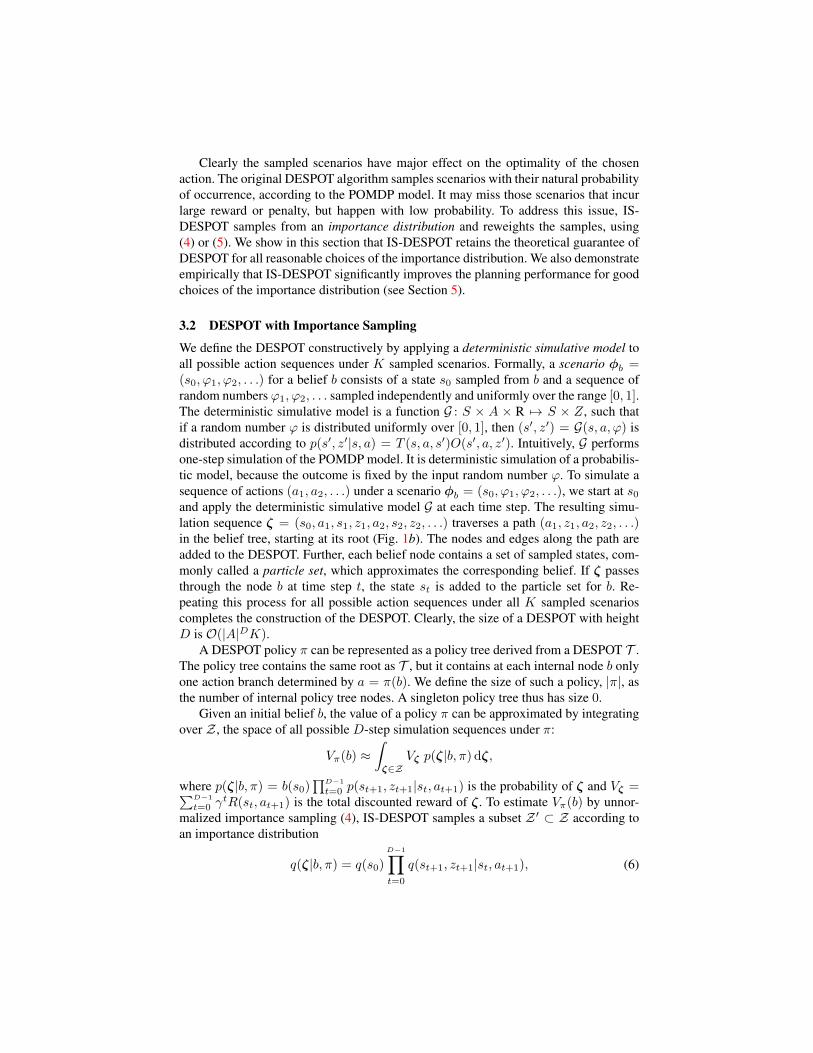
We define the DESPOT constructively by applying a deterministic simulative model toall possible action sequences under K sampled scenarios. Formally, a scenario φb =(s0, ϕ1, ϕ2, . . .) for a belief b consists of a state s0 sampled from b and a sequence ofrandom numbers ϕ1, ϕ2, . . . sampled independently and uniformly over the range [0, 1].The deterministic simulative model is a function G : S × A × R 7→ S × Z, such thatif a random number ϕ is distributed uniformly over [0, 1], then (s′, z′) = G(s, a, ϕ) isdistributed according to p(s′, z′|s, a) = T (s, a, s′)O(s′, a, z′). Intuitively, G performsone-step simulation of the POMDP model. It is deterministic simulation of a probabilis-tic model, because the outcome is fixed by the input random number ϕ. To simulate asequence of actions (a1, a2, . . .) under a scenario φb = (s0, ϕ1, ϕ2, . . .), we start at s0and apply the deterministic simulative model G at each time step. The resulting simu-lation sequence ζ = (s0, a1, s1, z1, a2, s2, z2, . . .) traverses a path (a1, z1, a2, z2, . . .)in the belief tree, starting at its root (Fig. 1b). The nodes and edges along the path areadded to the DESPOT. Further, each belief node contains a set of sampled states, com-monly called a particle set, which approximates the corresponding belief. If ζ passesthrough the node b at time step t, the state st is added to the particle set for b. Re-peating this process for all possible action sequences under all K sampled scenarioscompletes the construction of the DESPOT. Clearly, the size of a DESPOT with heightD is O(|A|DK).

A DESPOT policy π can be represented as a policy tree derived from a DESPOT T .The policy tree contains the same root as T , but it contains at each internal node b onlyone action branch determined by a = π(b). We define the size of such a policy, |π|, asthe number of internal policy tree nodes. A singleton policy tree thus has size 0.

Given an initial belief b, the value of a policy π can be approximated by integratingover Z , the space of all possible D-step simulation sequences under π:

Vπ(b) ≈∫ζ∈Z

Vζ p(ζ|b, π) dζ,

where p(ζ|b, π) = b(s0)∏D−1

t=0 p(st+1, zt+1|st, at+1) is the probability of ζ and Vζ =∑D−1

t=0 γtR(st, at+1) is the total discounted reward of ζ. To estimate Vπ(b) by unnor-

malized importance sampling (4), IS-DESPOT samples a subset Z ′ ⊂ Z according toan importance distribution

q(ζ|b, π) = q(s0)

D−1∏t=0

q(st+1, zt+1|st, at+1), (6)

where q(s0) is the distribution for sampling the initial state and q(st+1, zt+1|st, at+1)is the distribution for sampling the state transitions and observations. Then,

V̂π(b) =1

|Z ′|∑ζ∈Z′

w(ζ)Vζ =1

|Z ′|∑ζ∈Z′

D−1∑t=0

w(ζ0:t)γtR(st, at+1), (7)

where w(ζ) = p(ζ|b, π)/q(ζ|b, π) is the importance weight of ζ, ζ0:t is a subsequenceof ζ over the time steps 0, 1, . . . , t, and w(ζ0:t) is the importance weight of ζ0:t.

To avoid over-fitting to the sampled scenarios, IS-DESPOT optimizes a regularizedobjective function:

maxπ∈ΠT

{V̂π(b)− λ|π|

}, (8)

where ΠT is the set of all policy trees derived from a DESPOT T and λ ≥ 0 is regular-ization constant. More details on the benefits of regularization are available in [26].

3.3 Online Planning

IS-DESPOT is an online POMDP planning algorithm. At each time step, IS-DESPOTsearches a DESPOT T rooted at the current belief b0. It obtains a policy π that opti-mizes (8) at b0 and chooses the action a = π(b0) for execution.

To optimize (8), we substitute (7) into (8) and define the regularized weighted dis-counted utility (RWDU) of a policy π at each DESPOT node b:

νπ(b) =1

|Z ′|

∑ζ∈Z′b

D−1∑t=∆(b)

w(ζ0:t)γtR(st, at+1)− λ|πb|, (9)

where Z ′b ⊂ Z ′ contains all simulation sequences traversing paths in T through thenode b; ∆(b) is the depth of b in T ; πb is the subtree of π with the root b. Given a policyπ, there is one-to-one correspondence between scenarios and simulation sequences. So,|Z ′| = K. We optimize νπ(b0) overΠT by performing a tree search on T and applyingBellman’s equation recursively at every internal node of T , similar to (3):

ν∗(b) = max

{γ∆(b)

K

∑ζ∈Z′b

w(ζ0:∆(b))Vπ0,sζ,∆(b), maxa∈A

{ρ(b, a)+

∑z∈Zb,a

ν∗(τ(b, a, z))}}

(10)where

ρ(b, a) =1

K

∑ζ∈Z′b

γ∆(b)w(ζ0:∆(b))R(sζ,∆(b), a)− λ.

In (10), π0 denotes a given default policy; sζ,∆(b) denotes the state in ζ at time step∆(b); Vπ0,s is the value of π0 starting from a state s. At each node b, we may choose tofollow a default policy π0 or one of the action branches. The out maximization in (10)chooses between these two options, while the inner maximization chooses the specificaction branch. The maximizer at b0, the root of T , gives the optimal action.

There are many tree search algorithms. One is to traverse T from the bottom up.At each leaf node b of T , the algorithm sets ν∗(b) as the value of the default policy π0

and then applies (10) at each internal node until reaching the root of T . The bottom-uptraversal is conceptually simple, but T must be constructed fully in advance. For verylarge POMDPs, the required number of scenarios, K, may be huge, and constructingthe full DESPOT is not practical.

To scale up, an alternative is to perform anytime heuristic search. To guide theheuristic search, the algorithm maintains at each node b of T a lower bound and anupper bound on ν∗(b). It constructs and searches T incrementally, using K sampledscenarios. Initially, T contains only a single root node with belief b0. The algorithmmakes a series of explorations to expand T and reduces the gap between the upper andlower bounds at the root node b0 of T . Each exploration follows the heuristic and tra-verses a promising path from b0 to add new nodes at the end of the path. The algorithmthen traces the path back to b0 and applies (10) to both the lower and upper bounds ateach node along the way. The explorations continue, until the gap between the upperand lower bounds reaches a target level or the allocated online planning time runs out.

Online planning for IS-DESPOT is very similar to that for DESPOT. We refer thereader to [26] for details.

3.4 Analysis

We now show that IS-DESPOT retains the theoretical guarantee of DESPOT. The twotheorems below generalize the earlier results [22] to the case of importance sampling.To simplify the presentation, this analysis assumes, without loss of generality,R(s, a) ∈[0, Rmax] for all states and actions. All proofs are available in the appendix.

Theorem 1 shows that with high probability, importance sampling produces an ac-curate estimate of the value of a policy.

Theorem 1. Let b0 be a given belief. Let ΠT be the set of all IS-DESPOT policies de-rived from a DESPOT T and Πb0,D,K =

⋃T ΠT be the union over all DESPOTs with

root node b0, with height D, and constructed with all possible K importance-sampledscenarios. For any τ, α ∈ (0, 1), every IS-DESPOT policy π ∈ Πb0,D,K satisfies

Vπ(b0) ≥1− α1 + α

V̂π(b0)−RmaxWmax

(1 + α)(1− γ)· ln(4/τ) + |π| ln(KD|A||Z|)

αK(11)

with probability at least 1− τ , where

Wmax =

{maxs,s′∈Sa∈A,z∈Z

p(s, z|s′, a)q(s, z|s′, a)

}Dis the maximum importance weight.

The estimation error bound in (11) holds for all policies in Πb0,D,K simultaneously. Italso holds for any constant α ∈ (0, 1), which is a parameter that can be tuned to tightenthe bound. The additive error on the RHS of (11) depends on the size of policy π. Italso grows logarithmically with |A| and |Z|, indicating that IS-DESPOT scales up wellfor POMDP with very large action and observation spaces.

Theorem 2 shows that we can find a near-optimal policy π̂ by maximizing the RHSof (11).

Theorem 2. Let π∗ be an optimal policy at a belief b0. Let ΠT be the set of policiesderived from a DESPOT T that has height D and is constructed with K importance-sampled scenarios for b0. For any τ, α ∈ (0, 1), if

π̂ = argmaxπ∈ΠT

{1− α1 + α

V̂π(b0)−RmaxWmax

(1 + α)(1− γ)· |π| ln(KD|A||Z|)

αK

},

then with probability at least 1− τ ,

Vπ̂(b0) ≥1− α1 + α

Vπ∗(b0)−RmaxWmax

(1 + α)(1− γ)

×

(ln(8/τ) + |π∗| ln(KD|A||Z|)

αK+ (1− α)

(√2 ln(2/τ)

K+ γD

)).

(12)

The estimation errors in both theorems depend on the choice of the importancedistribution. By setting the importance sampling distribution to the natural probabil-ity of occurrence, we recover exactly the same results for the original DESPOT algo-rithm [22].

3.5 Normalized Importance Sampling

As we discussed in Section 2.2, normalized importance sampling often reduces the vari-ance of an estimator in practice. The algorithm remains basically the same, other thannormalizing the importance weights. The analysis is also similar, but is more involved.Our experiments show that IS-DESPOT with normalized importance weights producesbetter performance in some cases (see Section 5).

4 Importance Distributions

We now derive the optimal importance distribution for IS-DESPOT and then present ageneral method for learning it. We focus on the importance distribution for samplingstate transitions and leave that for sampling observations as future work.

4.1 Optimal Importance Distribution

The value of a policy π at a belief b, Vπ(b), is the expected total discounted rewardof executing π, starting at a state s distributed according to b. It can be obtained byintegrating over all possible starting states:

Vπ(b) =

∫s∈S

E(v|s, π)b(s) ds,

where v is a random variable representing the total discounted reward of executing πstarting from s and E(v|s, π) is its expectation. Compared with standard importancesampling (Section 2.2), IS-DESPOT estimates f(s) = E(v|s, π) by Monte Carlo simu-lation of π rather than evaluates f(s) deterministically. Thus the importance distribution

must account for not only the mean E(v|s, π) but also the variance Var(v|s, π) result-ing from Monte Carlo Sampling, and give a state s increased importance when either islarge. The theorem below formalizes this idea.

Theorem 3. Given a policy π, let v be a random variable representing the total dis-counted reward of executing π, starting from state s, and let Vπ(b) be the expected totaldiscounted reward of π at a belief b. To estimate Vπ(b) using unnormalized importancesampling, the optimal importance distribution is q∗π(s) = b(s)/wπ(s), where

wπ(s) =Eb(√

[E(v|s, π)]2 +Var(v|s, π))

√[E(v|s, π)]2 +Var(v|s, π)

. (13)

Theorem 3 specifies the optimal importance distribution for a given policy π, butIS-DESPOT must evaluate many policies within a set ΠT , for some DESPOT T . Ournext result suggests that we can use the optimal importance distribution for a policyπ to estimate the value of another “similar” policy π′. This allows us to use a singleimportance distribution for IS-DESPOT.

Theorem 4. Let V̂π,q(b) be the estimated value of a policy π at a belief b, obtained byK independent samples with importance distribution q. Let v be the total discountedreward of executing a policy π, starting from a state s ∈ S. If two policies π and π′

satisfy Var(v|s,π′)Var(v|s,π) ≤ 1 + ε and [E(v|s,π′)]

2

[E(v|s,π)]2 ≤ 1 + ε for all s ∈ S and some ε > 0, then

Var(V̂π′,q∗π (b)

)≤ (1 + ε)

(Var(V̂π,q∗π (b)) +

1

KV ∗(b)2

), (14)

where q∗π is an optimal importance distribution for estimating the value of π and V ∗(b)is the value of an optimal policy at b.

4.2 Learning Importance Distributions

According to Theorems 3 and 4, we can construct the importance distribution for IS-DESPOT, if we know the mean E(v|s, π) and the variance Var(v|s, π) for all s ∈ Sunder a suitable policy π ∈ ΠT . Two issues remain. First, we need to identify π.Second, we need to represent E(v|s, π) and Var(v|s, π) compactly, as the state space Smay be very large or even continuous. For the first issue, we use the policy generated bythe DESPOT algorithm, without importance sampling. Theorem 4 helps to justify thischoice. For the second issue, we use offline learning, based on discrete feature mapping.Specifically, we learn the function

ξ(s) =

√[E(v|s, π)]2 +Var(v|s, π), (15)

which is proportional to the inverse importance weight 1/wπ(s). We then set the im-portance distribution to q(s) = ηp(s) ξ(s), where η is the normalization constant.

To learn ξ(s), we first generate data by running DESPOT many times offline insimulation without importance sampling. Each run starts at a state s0 sampled fromthe initial belief b0 and generates a sequence {s0, a1, r1, s1, a2, r2, s2, . . . , aD, rD, sD},

where at is the action that DESPOT chooses, st is a state sampled from the modelp(st|st−1, at) = T (st−1, at, st), and rt = R(st−1, at) is the reward at time t fort = 1, 2, . . . . Let vt =

∑Di=t γ

(i−t)ri be the total discounted reward from time t. Wecollect all pairs (st−1, vt) for t = 1, 2, . . . from each run. Next, we manually constructa set of features over the state space S so that each state s ∈ S maps to its feature valueF(s). Finally, We discretize the feature values into a finite set of bins of equal size andinsert each collected data pair (s, v) into the bin that contains F(s). We calculate themean E(v) and the variance Var(v) for each bin. For any state s ∈ S, ξ(s) can then beapproximated from the mean and the variance of the bin that contains F(s).

This learning method scales up to high-dimensional and continuous state spaces,provided a small feature set can be constructed. It introduces approximation error, as aresult of discretization. However, the importance distribution is a heuristic that guidesMonte Carlo sampling, and IS-DESPOT is overall robust against approximation errorin the importance distribution. The experimental results in the next section show thatthe importance distribution captured by a small feature set effectively improves onlineplanning for large POMDPs.

5 Experiments

We evaluated IS-DESPOT on a suite of five tasks (Table 1). The first three tasks areknown to contain critical states, states which are not encountered frequently, but maylead to significant consequences. The other two, RockSample [21] and Pocman [19],are established benchmark tests for evaluating the scalability of POMDP algorithms.

We compared two versions of IS-DESPOT, unnormalized and normalized, with bothDESPOT and POMCP. See Table 1 for the results. For all algorithms, we set the max-imum online planning time to one second per step. For DESPOT and IS-DESPOT, weset the number of sampled scenarios to 500 and used an uninformative upper boundand fixed-action lower bound policy without domain-specific knowledge [26] in Asym-metricTiger, CollisionAvoidance, and Demining. Following earlier work [26], we setthe number of sampled scenarios to 500 and 100, respectively, in RockSample and Poc-man, and used domain-specific heuristics. For fair comparison, we tuned the explorationconstant of POMCP to the best possible and used a rollout policy with the same domainknowledge as that for DESPOT and IS-DESPOT in each task.

Overall, Table 1 shows that both unnormalized and normalized IS-DESPOT sub-stantially outperform DESPOT and POMCP in most tasks, including, in particular, thetwo large-scale tasks, Demining and Pocman. Normalized IS-DESPOT performs betterthan unnormalized IS-DESPOT in some tasks, though not all.

AsymmetricTiger Tiger is a classic POMDP [9]. A tiger hides behind one of twodoors, denoted by states sL and sR, with equal probabilities. An agent must decidewhich door to open, receiving a reward of +10 for opening the door without the tigerand receiving −100 otherwise. At each step, the agent may choose to open a door or tolisten. Listening incurs a cost of−1 and provides the correct information with probabil-ity 0.85. The task resets once the door is opened. The only uncertainty here is the tiger’slocation. Tiger is a toy problem, but it captures the key trade-off between information

Table 1: Performance comparison. The table shows the average total discounted rewards(95% confidence interval) of four algorithms on five tasks. UIS-DESPOT and NIS-DESPOT refer to unnormalized and normalized IS-DESPOT, respectively.

AsymmetricTiger CollisionAvoidance Demining RockSample(15,15) Pocman

|S| 2 9,720 ∼ 1049 7,372,800 ∼ 1056

|A| 3 3 9 20 4|Z| 2 18 16 3 1,024POMCP −5.60± 1.51 −4.19± 0.07 −17.11± 2.74 15.32± 0.28 294.16± 4.06DESPOT −2.20± 1.78 −1.05± 0.27 −11.09± 2.45 18.37± 0.28 317.90± 4.17UIS-DESPOT 3.70± 0.49 −0.87± 0.19 − 3.45± 1.76 18.30± 0.32 315.13± 4.92NIS-DESPOT 3.75± 0.47 −0.44± 0.12 − 3.69± 1.80 18.68± 0.28 326.92± 3.89

state E(v|s) Var(v|s) p(s) q(s)

sL 4.36 7.34 0.99 0.40

sR −65.84 566978.9 0.01 0.600 100 200 300 400 500

K

100

80

60

40

20

0

20

aver

age

tota

l dis

coun

ted

rew

ard

OptimalDESPOTUIS-DESPOTNIS-DESPOT

0 100 200 300 400 500K

0.000

0.002

0.004

0.006

0.008

0.010

rate

of g

ettin

g -1

0000

pen

alty DESPOT

UIS-DESPOTNIS-DESPOT

(a) (b) (c)

Fig. 2: AsymmetricTiger. (a) Importance distribution q. DESPOT samples accordingto p. IS-DESPOT samples according to q. (b) Average total discounted reward versusK, the number of sampled scenarios. (c) The rate of opening the door with the tigerbehind versus K.

gathering and information exploitation prevalent in robot planning under uncertainty.We use it to gain understanding on some important properties of IS-DESPOT.

We first modify the original Tiger POMDP. Instead of hiding behind the two doorswith equal probabilities, the tiger hides behind the right door with much smaller prob-ability 0.01. However, if the agent opens the right door with the tiger hiding there, thepenalty increases to −10, 000. Thus the state sR occurs rarely, but has a significantconsequence. Sampling sR is crucial.

Since this simple task only has two states, we learn the weight for each state anduse them to construct the importance distribution for IS-DESPOT (Fig. 2a).

Table 1 shows clearly that both versions of IS-DESPOT significantly outperformDESPOT and POMCP. This is not surprising. DESPOT and POMCP sample the twostates sL and sR according to their natural probabilities of occurrence and fail to ac-count for their significance, in this case, the high penalty of sR. As a result, they rarelysample sR. In contrast, the importance distribution enables IS-DSPOT to sample sRmuch more frequently (Fig. 2a). Unnormalized and normalized IS-DESPOT are similarin performance, as normalization has little effect on this small toy problem.

We conducted additional experiments to understand howK, the number of sampledscenarios, affects performance (Fig. 2b, c). To calibrate the performance, we ran an of-fline POMDP algorithm SARSOP [15] to compute an optimal policy. WhenK is small,the performance gap between DESPOT and IS-DESPOT is significant. As K increases,the gap narrows. When K is 32, both versions of IS-DESPOT are near-optimal, while

0 100 200 300 400 500K

9876543210

aver

age

tota

l dis

coun

ted

rew

ard

DESPOTUIS-DESPOTNIS-DESPOT

0 100 200 300 400 500K

0.000

0.005

0.010

0.015

0.020

0.025

0.030

0.035

collis

ion

rate

DESPOTUIS-DESPOTNIS-DESPOT

0 2 4 6 8 10 12 14 16 18dy

05

1015202530354045

ξ(dx,dy)

dx =5

dx =6

dx =25

(a) (b) (c) (d)Fig. 3: CollisionAvoidance. (a) An aircraft changes the direction to avoid collision. (b)Average total discounted reward versus K, the number of scenarios. (c) Collision rateversus K. (d) ξ(dx, dy) learned from data.

DESPOT does not reach a comparable performance level even at K = 500. All theseconfirm the value of importance sampling for small sample size.

One may ask how DESPOT and IS-DESPOT compare on the original Tiger task.The original Tiger has two symmetric states. The optimal importance distribution is flat.Thus DESPOT and IS-DESPOT have the same sampling distribution, and IS-DESPOThas no performance advantage over DESPOT. Importance sampling is beneficial onlyif the planning task involves significant events of low probability.

CollisionAvoidance This is an adaptation of the aircraft collision avoidance task [2].The agent starts moving from a random position in the right-most column of a 18 ×30 grid map (Fig. 3a). An obstacle randomly moves in the left-most column of thismap: moves up with probability 0.25, down with 0.25, and stay put with 0.50. Theprobabilities become 0, 0.25, and 0.75 respectively when the obstacle is at the top-most row, and become 0.25, 0, and 0.75 respectively when it is at the bottom-most row.Each time, the agent can choose to move upper-left, lower-left or left, with a cost of−1, −1, and 0 respectively. If the agent collides with the obstacle, it receives a penaltyof −1, 000. The task finishes when the agent reaches the left-most column. The agentknows its own position exactly, but observes the obstacle’s position with a Gaussiannoise N (0, 1). The probability of the agent colliding with the obstacle is small, but thepenalty of collision is high.

To construct the importance distribution for IS-DESPOT, we map a state s to a fea-ture vector (dx, dy) and learn ξ(dx, dy). The features dx and dy are the horizontal andvertical distances between the obstacle and the agent respectively. The horizontal dis-tance dx is the number of steps remaining for the agent to move, and (dx, dy) = (0, 0)represents a collision. These features capture the changes in the mean and variance ofpolicy values for different states, because when the agent is closer to the obstacle, theprobability of collision is higher, which leads to worse mean and larger variance.

Fig. 3d plots ξ(dx, dy) for a few chosen horizontal distance dx: ξ(dx = 5, dy),ξ(dx = 6, dy) and ξ(dx = 25, dy). Overall, ξ(dx, dy) is higher when the obstacleis closer to the agent. At dx = 5, ξ(dx, dy) is close to zero for all dy >= 4, andξ(dx, dy) = 0 when dy >= 10. This indicates that the DESPOT policy rarely causescollisions when the vertical distance is larger than 4, because the collision would re-quire the agent and obstacle move towards each other for several steps in the remainingdx = 5 steps, which is unlikely to happen since the DESPOT policy is actively avoidingthe collision. Furthermore, collision is not possible at all when dy >= 10 because it

100 150 200 250 300 350 400 450 500K

70

60

50

40

30

20

10

0

aver

age

tota

l dis

coun

ted

rew

ard

DESPOTUIS-DESPOTNIS-DESPOT

100 150 200 250 300 350 400 450 500K

0.020.040.060.080.100.120.140.160.180.20

expl

osio

n ra

te

DESPOTUIS-DESPOTNIS-DESPOT

(a) (b) (c)Fig. 4: Demining. (a) A robot moves in a 10 × 10 map to detect and report landmines.(b) Average total discounted reward versus K, the number of scenarios. (c) The rate ofhitting mines versus K.

requires at least 6 steps for the agent and the obstacle to meet. With this importancedistribution, IS-DESPOT can ignore the states that do not cause collision and focuson sampling states that likely lead to collisions. This could significantly improve theconvergence rate, as shown in Fig. 3b and Fig. 3c : IS-DESPOT performs better thanDESPOT with small K. NIS-DESPOT improves the performance further. It also per-forms well with small K, while DESPOT cannot reach the same level of performanceeven with a large K.Demining This is an adapted version of the robotic de-mining task in HumanitarianRobotics and Automation Technology Challenge (HRATC) 2015 [27]. It requires anagent to sweep a 10× 10 grid field to detect and report landmines. Each grid cell has amine with probability 0.05. At each time step, the agent can move in four directions, andthen observe the four adjacent cells with 0.9 accuracy. DESPOT is a core componentof the system winning HRATC 2015. We show that IS-DESPOT handles critical statesin the task better than DESPOT, resulting in better performance overall. If the agentreports the mine correctly, it receives reward +10, and −10 otherwise. Stepping overthe mine causes high penalty −1, 000 and task termination, which is a critical state.

To construct the importance distribution for IS-DESPOT, we map a state s to afeature vector (n, d) and learn ξ(n, d), where n is the number of unreported mines andd is the Manhattan distance between the agent and the nearest mine. These two featurescapture the changes in the mean and variance of the rollout values for different states,because n determines the maximum total discounted rewards that the agent can get, andd affects the probability of stepping over mines.

Fig. 4b shows the performance comparison between IS-DESPOT and DESPOT fordifferent number of scenarios K. IS-DESPOT converges faster than DESPOT, and sig-nificantly outperforms DESPOT even for relatively large number of scenarios (K =500). Fig. 4c shows that the performance improvement results from a decrease in thenumber of explosions. For this task, the size of the state space is about 1049, and IS-DESPOT clearly outperforms DESPOT and POMCP (Table 1), affirming the scalabilityof IS-DESPOT.RockSample RockSample is a standard POMDP benchmark problem [21]. In the prob-lemRockSample(n, k), the agent moves on an n×n grid map which has k rocks. Eachof the rocks can either be good or bad. The agent knows each rock’s position but doesnot know its state (good or bad). At each time step, the agent can choose to observe thestates, move, or sample. The agent can sample a rock it steps on, and get a reward of

Fig. 5: RockSample. A robot senses rocks to identify “good” ones and samples them.Upon completion, it exits the east boundary.

+10 if the rock is good, −10 otherwise. A rock turns bad after being sampled. Movingor sensing has no cost. The agent can sense the state of the rock with accuracy decreas-ing exponentially with respect to the distance to the rock. When the agent exits fromthe east boundary of the map, it gets a reward of +10 and the task terminates.

To construct the importance distribution for IS-DESPOT, we map a state s to a fea-ture vector (n, d+, d−), where n is the number of remaining good rocks, d+ and d− arethe Manhattan distances to the nearest good rock and the nearest bad rock respectively.This task does not contain critical states, nevertheless, IS-DESPOT maintains the samelevel of performance as DESPOT (Table 1).

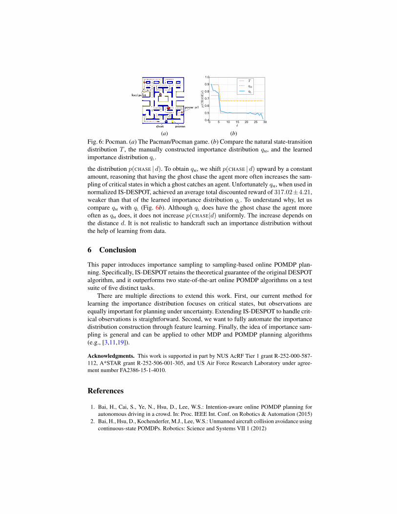
Pocman Pocman [19] is a partially observable variant of the popular Pacman game(Fig. 6a). An agent and four ghosts move in a 17×19 maze populated with food pallets.The agent can move from a cell in the maze to an adjacent one if there is no wall inbetween. Each move incurs a cost of−1. A cell contains the food pallet with probability0.5. Eating a food pallet gives the agent a reward of +10. Getting caught by ghostsincurs a penalty of −100. There are four power pills. After eating a power pill, theagents retains it for the next 15 steps and acquires the power to kill ghosts. Killing aghost gives a reward of +25. Let d be the Manhattan distance between the agent and aghost. When d ≤ 5, the ghost chases the agent with probability 0.75 if the agent doesnot possess the power pill; the ghost runs away, but slips with probability 0.25 if theagent possesses the power pill. When d > 5, the ghost moves uniformly at random tofeasible adjacent cells. In contrast with that in the original Pacman game, the Pocmanagent does not know the exact locations of ghosts, but sees approaching ghosts whenthey are in a direct line of sight and hears them when d ≤ 2.

To construct the importance distribution for IS-DESPOT, we map a state s to afeature vector (n, dmin),where dmin is the Manhattan distance to the nearest ghost andn is the number of remaining steps for which the agent retains a power pill.

Table 1 shows that unnormalized IS-DESPOT does not bring in improvement overDESPOT. However, normalized IS-DESPOT does, because normalization of impor-tance weight reduces variance in this case.

To understand the benefits of learning the importance distribution, we tried to con-struct an importance distribution qM manually. The states, in which a ghost catches theagent, are critical. They do not occur very often, but incur high penalty. An effectiveimportance distribution must sample such states with increased probability. One cru-cial aspect of the ghost behaviour is the decision of chasing the agent, governed by

0 5 10 15 20 25 30d

0.4

0.5

0.6

0.7

0.8

0.9

1.0

p(C

HA

SE|d

)

T

qMqL

(a) (b)Fig. 6: Pocman. (a) The Pacman/Pocman game. (b) Compare the natural state-transitiondistribution T , the manually constructed importance distribution qM, and the learnedimportance distribution qL.

the distribution p(CHASE | d). To obtain qM, we shift p(CHASE | d) upward by a constantamount, reasoning that having the ghost chase the agent more often increases the sam-pling of critical states in which a ghost catches an agent. Unfortunately qM, when used innormalized IS-DESPOT, achieved an average total discounted reward of 317.02±4.21,weaker than that of the learned importance distribution qL. To understand why, let uscompare qM with qL (Fig. 6b). Although qL does have the ghost chase the agent moreoften as qM does, it does not increase p(CHASE|d) uniformly. The increase depends onthe distance d. It is not realistic to handcraft such an importance distribution withoutthe help of learning from data.

6 Conclusion

This paper introduces importance sampling to sampling-based online POMDP plan-ning. Specifically, IS-DESPOT retains the theoretical guarantee of the original DESPOTalgorithm, and it outperforms two state-of-the-art online POMDP algorithms on a testsuite of five distinct tasks.

There are multiple directions to extend this work. First, our current method forlearning the importance distribution focuses on critical states, but observations areequally important for planning under uncertainty. Extending IS-DESPOT to handle crit-ical observations is straightforward. Second, we want to fully automate the importancedistribution construction through feature learning. Finally, the idea of importance sam-pling is general and can be applied to other MDP and POMDP planning algorithms(e.g., [3,11,19]).

Acknowledgments. This work is supported in part by NUS AcRF Tier 1 grant R-252-000-587-112, A*STAR grant R-252-506-001-305, and US Air Force Research Laboratory under agree-ment number FA2386-15-1-4010.

References

1. Bai, H., Cai, S., Ye, N., Hsu, D., Lee, W.S.: Intention-aware online POMDP planning forautonomous driving in a crowd. In: Proc. IEEE Int. Conf. on Robotics & Automation (2015)

2. Bai, H., Hsu, D., Kochenderfer, M.J., Lee, W.S.: Unmanned aircraft collision avoidance usingcontinuous-state POMDPs. Robotics: Science and Systems VII 1 (2012)

3. Bai, H., Hsu, D., Lee, W.S., Ngo, V.A.: Monte Carlo value iteration for continuous-statePOMDPs. In: Algorithmic Foundations of Robotics IX (2010)

4. Folsom-Kovarik, J., Sukthankar, G., Schatz, S.: Tractable POMDP representations for intel-ligent tutoring systems. ACM Trans. on Intelligent Systems & Technology 4(2) (2013)

5. Gelly, S., Silver, D.: Combining online and offline knowledge in UCT. In: Proc. Int. Conf.on Machine Learning (2007)

6. Glasserman, P.: Monte Carlo methods in financial engineering, vol. 53. Springer Science &Business Media (2003)

7. He, R., Brunskill, E., Roy, N.: Efficient planning under uncertainty with macro-actions. J.Artificial Intelligence Research 40(1) (2011)

8. Hsiao, K., Kaelbling, L.P., Lozano-Perez, T.: Grasping POMDPs. In: Proc. IEEE Int. Conf.on Robotics & Automation (2007)

9. Kaelbling, L.P., Littman, M.L., Cassandra, A.R.: Planning and acting in partially observablestochastic domains. Artificial Intelligence 101(1) (1998)

10. Kalos, M., Whitlock, P.: Monte Carlo Methods, vol. 1. John Wiley & Sons, New York (1986)11. Kearns, M., Mansour, Y., Ng, A.Y.: A sparse sampling algorithm for near-optimal planning

in large Markov decision processes. Machine Learning 49(2-3) (2002)12. Koller, D., Friedman, N.: Probabilistic graphical models: principles and techniques. MIT

press (2009)13. Koval, M., Pollard, N., Srinivasa, S.: Pre- and post-contact policy decomposition for planar

contact manipulation under uncertainty. Int. J. Robotics Research 35(1–3) (2016)14. Koval, M., Hsu, D., Pollard, N., Srinivasa, S.: Configuration lattices for planar contact ma-

nipulation under uncertainty. In: Algorithmic Foundations of Robotics XII—Proc. Int. Work-shop on the Algorithmic Foundations of Robotics (WAFR) (2016)

15. Kurniawati, H., Hsu, D., Lee, W.S.: SARSOP: efficient point-based POMDP planning byapproximating optimally reachable belief spaces. In: Proc. Robotics: Science & Systems(2008)

16. Owen, A.B.: Monte Carlo theory, methods and examples (2013)17. Pineau, J., Gordon, G., Thrun, S.: Point-based value iteration: An anytime algorithm for

POMDPs. In: Proc. Int. Jnt. Conf. on Artificial Intelligence (2003)18. Ross, S., Pineau, J., Paquet, S., Chaib-Draa, B.: Online planning algorithms for POMDPs. J.

Artificial Intelligence Research 32 (2008)19. Silver, D., Veness, J.: Monte-Carlo planning in large POMDPs. In: Advances in Neural In-

formation Processing Systems (NIPS) (2010)20. Smallwood, R., Sondik, E.: The optimal control of partially observable Markov processes

over a finite horizon. Operations Research 21 (1973)21. Smith, T., Simmons, R.: Heuristic search value iteration for POMDPs. In: Proc. Uncertainty

in Artificial Intelligence (2004)22. Somani, A., Ye, N., Hsu, D., Lee, W.S.: DESPOT: Online POMDP planning with regulariza-

tion. In: Advances in Neural Information Processing Systems (NIPS) (2013)23. Spaan, M., Vlassis, N.: Perseus: Randomized point-based value iteration for POMDPs. J.

Artificial Intelligence Research 24 (2005)24. Veach, E.: Robust Monte Carlo methods for light transport simulation. Ph.D. thesis, Stanford

University (1997)25. Wu, K., Lee, W.S., Hsu, D.: POMDP to the rescue: Boosting performance for RoboCup

rescue. In: Proc. IEEE/RSJ Int. Conf. on Intelligent Robots & Systems (2015)26. Ye, N., Somani, A., Hsu, D., Lee, W.S.: DESPOT: Online POMDP planning with regulariza-

tion. J. Artificial Intelligence Research (to appear)27. Humanitarian robotics and automation technology challenge (HRATC) 2015, http://

www.isr.uc.pt/HRATC2015

A Proofs

A.1 Theorems 1 and 2

To prove Theorem 1, we rely on an earlier result [22]:

Theorem 5. For any τ, α ∈ (0, 1), every policy tree π ∈ Πb0,D,K satisfies

Vπ(b0) ≥1− α1 + α

V̂π(b0)−Rmax

(1 + α)(1− γ)· ln(4/τ) + |π| ln(KD|A||Z|)

αK,

with probability at least 1 − τ , where V̂π(b0) is the estimated value of π under any setof K randomly sampled scenarios for belief b0.

The theorem above is similar to Theorem 1, but provides the performance guarantee forthe original DESPOT algorithm, which does not employ importance sampling. Thereare two key differences. When computing V̂π(b0) without importance sampling, we usethe natural state-transition and observation probability distribution p(st+1, zt+1|st, at+1)to generate the next state and observation in a simulation sequence ζ; with importancesampling, we use the importance distribution q(st+1, zt+1|st, at+1). Further, withoutimportance sampling, we use the reward R(st, at+1) from the POMDP model; withimportance sampling, we use the weighted reward w(ζ0:t)R(st, at+1), where ζ is asimulation sequence that leads to st and w(ζ0:t) is the weight of the sub-sequence ofζ over the time steps 0, 1, ..., t. To prove Theorem 1, our general idea is to construct anew POMDP with modified dynamics and reward to account for importance samplingand then apply Theorem 5.

Proof. (Theorem 1) We construct a new POMDP with the state-transition and obser-vation probability distribution p′(st+1, zt+1|st, at+1) = q(st+1, zt+1|st, at+1) and re-ward functionR′(st, at+1) = w(ζ0:t)R(st, at+1). Running DESPOT algorithm on thisnew POMDP model and running IS-DESPOT on the original model generate exactlythe same simulation sequences with same total rewards. It then follows from Theorem 5that

V ′π(b0) ≥1− α1 + α

V̂π(b0)−R′max

(1 + α)(1− γ)· ln(4/τ) + |π| ln(KD|A||Z|)

αK, (16)

where V ′π(b0) is the value of π at b0 under the new model andR′max = maxs∈S,a∈AR′(s, a).

Note that

maxs∈S,a∈A

R′(s, a) = maxζ0:t

st∈S,at+1∈A

w(ζ0:t)R(st, at+1) ≤

{maxs,s′∈Sa∈A,z∈Z

p(s, z|s′, a)q(s, z|s′, a)

}tRmax.

Since Es,z∼q(s,z|s′,a) p(s,z|s′,a)

q(s,z|s′,a) = 1 for all s′ ∈ S and a ∈ A, we have

maxs,s′∈Sa∈A,z∈Z

p(s, z|s′, a)q(s, z|s′, a)

≥ 1.

Hence

R′max ≤

{maxs,s′∈Sa∈A,z∈Z

p(s, z|s′, a)q(s, z|s′, a)

}tRmax ≤

{maxs,s′∈Sa∈A,z∈Z

p(s, z|s′, a)q(s, z|s′, a)

}DRmax =WmaxRmax,

(17)as t ≤ D. Combining (16) and (17), we have

V ′π(b0) ≥1− α1 + α

V̂π(b0)−RmaxWmax

(1 + α)(1− γ)· ln(4/τ) + |π| ln(KD|A||Z|)

αK. (18)

It remains to show that π has the same value under the new and the original POMDPmodels. By definition,

V ′π(b0) = Eζ∼q(ζ|b0,π)

( ∞∑t=0

γtw(ζ0:t)R(st, at+1)

)

=

∫ ∞∑t=0

γtw(ζ0:t)R(st, at+1)q(ζ|b0, π) dζ

=

∞∑t=0

∫p(ζ0:t|b0, π)q(ζ0:t|b0, π)

γtR(st, at+1)q(ζ|b0, π) dζ.

Since the rewardR(st, at+1) does not depend on the subsequence ζt+1:∞, we marginal-ize it out and get

V ′π(b0) =

∞∑t=0

∫p(ζ0:t|b0, π)q(ζ0:t|b0, π)

γtR(st, at+1)q(ζ0:t|b0, π) dζ0:t

=

∞∑t=0

∫p(ζ0:t|b0, π)γtR(st, at+1) dζ0:t

=

∫ ∞∑t=0

γtR(st, at+1)p(ζ|b0, π) dζ

= Vπ(b0).

(19)

The third line above again follows from marginalization over the subsequence ζt+1:∞.Finally, putting together (18) and (19), we get the desired result. �

To prove Theorem 2, we use Theorem 1 and follow the same steps as the proof ofTheorem 2 in [22]. We omit the details here.

A.2 Theorem 3

Proof. Given a policy π, we want to estimate Vπ(b), the value of π at the belief b, withthe importance distribution q(s). The variance of the estimator b(s)q(s)v is

Var

(b(s)

q(s)v

∣∣∣∣π) = E(b(s)2

q(s)2v2∣∣∣∣π)− [E( b(s)q(s)

v

∣∣∣∣π)]2=

∫b(s)2

q(s)2v2p(v|s, π)q(s) dv ds−

[E(b(s)

q(s)v

∣∣∣∣π)]2=

∫b(s)2

q(s)

(∫v2p(v|s, π) dv

)ds−

[E(b(s)

q(s)v

∣∣∣∣π)]2=

∫b(s)2

q(s)

([E (v|s, π)]2 +Var(v|s, π)

)ds−

[E(b(s)

q(s)v

∣∣∣∣π)]2 .(20)

Substituting q∗π(s) =b(s)√

[E(v|s,π)]2+Var(v|s,π)Eb

(√[E(v|s,π)]2+Var(v|s,π)

) into (20), we get

Var

(b(s)

q∗π(s)v

∣∣∣∣π) = Eb(√

[E (v|s, π)]2 +Var(v|s, π))∫ √

[E (v|s, π)]2 +Var(v|s, π) b(s)ds−[E(b(s)

q∗π(s)v

∣∣∣∣π)]2=

[Eb(√

[E (v|s, π)]2 +Var(v|s, π))]2−[E(b(s)

q∗π(s)v

∣∣∣∣π)]2Unnormalized importance sampling is unbiased. Thus, for any arbitrary importancedistribution q(s),

E(b(s)

q∗π(s)v

∣∣∣∣π) = E(b(s)

q(s)v

∣∣∣∣π) ,and

Var

(b(s)

q∗π(s)v

∣∣∣∣π) =

[Eb(√

[E (v|s, π)]2 +Var(v|s, π))]2−[E(b(s)

q(s)v

∣∣∣∣π)]2=

[Eq(b(s)

q(s)

√[E (v|s, π)]2 +Var(v|s, π)

)]2−[E(b(s)

q(s)v

∣∣∣∣π)]2≤ Eq

(b(s)2

q(s)2

([E (v|s, π)]2 +Var(v|s, π)

))−[E(b(s)

q(s)v

∣∣∣∣π)]2=

∫b(s)2

q(s)

([E (v|s, π)]2 +Var(v|s, π)

)ds−

[E(b(s)

q(s)v

∣∣∣∣π)]2= Var

(b(s)

q(s)v

∣∣∣∣π) .The third line above follows because [E(X)]2 ≤ E(X2) for any random variable Xby the Cauchy-Schwarz inequality, and the last line follows from (20). Therefore, thevariance of the estimator with importance distribution q∗π(s) is no greater than that withany other importance distribution, and q∗π(s) is optimal. �

A.3 Theorem 4

Proof. By the definition of V̂π′,q∗π (b),

V̂π′,q∗π (b) =1

K

K∑i=1

b(si)

q∗π(si)vi, vi ∼ p(v|si, π′), si ∼ q∗π(s),

where p(v|si, π′) is the probability distribution over the value v of following policy π′

from the starting state si. Since the states are sampled independently,

Var(V̂π′,q∗π (b)

)=

1

KVarq∗π

(b(s)

q∗π(s)v

∣∣∣∣π′)

Similar to (20), we get

Var

(b(s)

q∗π(s)v

∣∣∣∣π′) =

∫b(s)2

q∗π(s)

([E(v|s, π′)]2 +Var(v|s, π′)

)ds− Vπ′(b)2

where Vπ′(b) = Eq∗π

(b(s)q∗π(s)

v

∣∣∣∣π′) is the value of policy π′ at b. Hence

Var(V̂π′,q∗π (b)

)=

1

K

{∫b(s)2

q∗π(s)

([E(v|s, π′)]2 +Var(v|s, π′)

)ds− Vπ′(b)2

}≤ 1

K

{(1 + ε)

∫b(s)2

q∗π(s)

([E (v|s, π)]2 +Var(v|s, π)

)ds− Vπ′(b)2

}The second line above follows from the given conditions: Var(v|s,π′)

Var(v|s,π) ≤ 1 + ε and

[E(v|s,π′)]2

[E(v|s,π)]2 ≤ 1 + ε for all s ∈ S and some ε > 0. Let Vπ(b) = E(

b(s)q∗π(s)

v

∣∣∣∣π).

Var

(b(s)

q∗π(s)v

∣∣∣∣π′) ≤ 1

K

{(1 + ε)

(∫b(s)2

q∗π(s)

([E (v|s, π)]2 +Var(v|s, π)

)ds− Vπ(b)2 + Vπ(b)

2

)− Vπ′(b)2

}Similar to (20), we have

∫ b(s)2

q∗π(s)

(E[v|s, π]2 +Var(v|s, π)

)ds−Vπ(b)2 = Var

( b(s)q∗π(s)

v|π).

Hence

Var

(b(s)

q∗π(s)v

∣∣∣∣π′) ≤ 1 + ε

KVarq∗π (

b(s)

q∗π(s)v|π) + 1

K

((1 + ε)Vπ(b)

2 − Vπ′(b)2)

= (1 + ε)Var(V̂π,q∗π (b)

)+

1

K

((1 + ε)Vπ(b)

2 − Vπ′(b)2)

≤ (1 + ε)Var(V̂π,q∗π (b)

)+

1 + ε

KV ∗(b)2

= (1 + ε)

(Var(V̂π,q∗π (b)) +

1

KV ∗(b)2

).

�