improved ant colony optimization algorithms for continuous and
TRANSCRIPT

Université Libre de BruxellesFaculté des Sciences AppliquéesCODE - Computers and Decision EngineeringIRIDIA - Institut de Recherches Interdisciplinaireset de Développements en Intelligence Artificielle
Improved ant colony optimization algorithmsfor continuous and mixed discrete-continuous
optimization problems
Tianjun LIAO
Superviseur:
Prof. Marco DORIGO and Dr. Thomas STÜTZLE
Rapport d’avancement de rechercheAnnée Académique 2010/2011


Abstract
The interest in using the Ant Colony Optimization (ACO) metaheuristic tosolve continuous or mixed discrete-continuous variable optimization prob-lems is increasing. One of the most popular Ant Colony Optimization (ACO)algorithms for the continuous domain is ACOR. In this thesis, we proposean incremental ant colony algorithm with local search for continuous opti-mization (IACOR-LS), and we present an ant colony optimization algorithmfor mixed discrete-continuous variable optimization problems (ACOMV).
We start by a detailed experimental analysis of ACOR and based onthe obtained insights on ACOR, we propose IACOR-LS. This mechanismconsists of a growing solution archive with a special initialization rule ap-plied to entrant solutions. The resulting algorithm, called IACOR, is thenhybridized with a local search procedure in order to enhance its search inten-sification. Automatic parameter tuning results show that IACOR-LS withLin-Yu Tseng’s Mtsls1 local search algorithm (IACOR-Mtsls1) significantlyoutperforms ACOR, and it is also competitive with state-of-the-art algo-rithms.
We also show how ACOR may be extended to mixed-variable optimiza-tion problems. The proposed ACOMV algorithm allows to declare each vari-able of the considered problem as continuous, ordered discrete or categoricaldiscrete. Based on the solution archive framework of ACOMV, a continu-ous relaxation approach (ACOMV-o), a native mixed-variable optimizationapproach (ACOMV-c), as well as ACOR are integrated to solve continuousand mixed-variable optimization problems. An additional contribution is anew set of artificial mixed-variable benchmark functions, which can simulatediscrete variables as ordered or categorical. After automatically tuning theparameters of ACOMV on artificial mixed-variable benchmark functions, wetest generic ACOMV on various real-world continuous and mixed-variableengineering optimization problems. A comparison to results from literatureproves ACOMV’s high performance, and demonstrates its effectiveness androbustness.


Acknowledgements
I thank Prof. Marco Dorigo and Dr. Thomas Stützle for affording me thechance to research at IRIDIA. I also thank Dr. Thomas Stützle and Marco A.Montes de Oca for their guidance and support that help me to conduct theresearch presented in this work. I also thank Dr. Manuel López-Ibáñez andJérémie Dubois-Lacoste for their improved implementation of Iterated-F-Race package. Special thanks go to Zhi Yuan and Marco A. Montes de Oca.Talking with them helps me avoid detours, which is very helpful for my workefficiency. I would also like to express my gratitude to Mohamed SaifullahHussin, Sabrina Oliveira and my colleagues at IRIDIA. Your kindness makesmy life so enjoyable here.
This work was supported by E-SWARM project funded ERC AdvancedGrant, and supported by Meta-X project funded by the Scientific ResearchDirectorate of the French Community of Belgium.


Statement
This work describes an original research carried out by the author. It hasnot been previously submitted to any other university for the award of anydegree. Nevertheless, some chapters of this thesis are partially based on pa-pers, together with other co-authors, which have been published, submittedor prepared for publication in the scientific literature.
Chapter 3 is based on the paper:T. Liao, M. Montes de Oca, D. Aydın, T. Stützle, and M. Dorigo. AnIncremental Ant Colony Algorithm with Local Search for Continuous Opti-mization. Proceedings of the Genetic and Evolutionary Computation Con-ference, GECCO 2011. N. Krasnogor et al. (Eds.) Dublin, Ireland. July2011. Accepted.Nominated for the best paper award in the Ant Colony Optimization andSwarm Intelligence track (three of four referees nominated it for the bestpaper award).
Chapter 4 is based on the paper:T. Liao, K. Socha, M. Montes de Oca, T. Stützle, and M. Dorigo. AntColony Optimization for Mixed-Variables Problems. IEEE Transaction onevolutionary computation. In preparation for submission.
Other related publications:T. Liao, M. Montes de Oca, and T. Stützle. Tuning Parameters acrossMixed Dimensional Instances: A Performance Scalability Study of Sep-G-CMA-ES. Proceedings of the Workshop on Scaling Behaviours of Landscapes,Parameters and Algorithms of the Genetic and Evolutionary ComputationConference (GECCO 2011). E. Özcan, A. J. Parkes, and J. Rowe. (Eds.)Dublin, Ireland. July 2011. Accepted.T. Liao, M. Montes de Oca, and T. Stützle. A Note on the Effects of Enforc-ing Bound Constraints on Algorithm Comparisons using the IEEE CEC’05Benchmark Function Suite, TR/IRIDIA/2011-010, IRIDIA, Université Li-bre de Bruxelles, Belgium, April 2011.


Contents
Abstract iii
Acknowledgements v
Statement vii
1 Introduction 1
2 Ant Colony Optimization 52.1 ACOR: Ant Colony Optimization for Continuous Domains . . 62.2 Further Investigation on ACOR . . . . . . . . . . . . . . . . . 8
3 An Incremental Ant Colony Algorithm with Local Search 153.1 The IACOR Algorithm . . . . . . . . . . . . . . . . . . . . . . 163.2 IACOR with Local Search . . . . . . . . . . . . . . . . . . . . 173.3 Experimental Study . . . . . . . . . . . . . . . . . . . . . . . 18
3.3.1 Parameter Settings . . . . . . . . . . . . . . . . . . . . 183.3.2 Experimental Results and Comparison . . . . . . . . . 21
3.4 Conclusions . . . . . . . . . . . . . . . . . . . . . . . . . . . . 23
4 Ant Colony Optimization for Mixed Variable Problems 294.1 Mixed-variable Optimization Problems . . . . . . . . . . . . . 304.2 ACOMV Heuristics for Mixed-Variable Optimization Problems 32
4.2.1 ACOMV framework . . . . . . . . . . . . . . . . . . . 324.2.2 Probabilistic Solution Construction for Continuous Vari-
ables . . . . . . . . . . . . . . . . . . . . . . . . . . . . 324.2.3 Probabilistic Solution Construction for Ordered Dis-
crete Variables . . . . . . . . . . . . . . . . . . . . . . 334.2.4 Probabilistic Solution Construction for Categorical Vari-
ables . . . . . . . . . . . . . . . . . . . . . . . . . . . . 344.2.5 Auxiliary Explanations of ACOMV . . . . . . . . . . . 36
4.3 Artificial Mixed-variable Benchmark Functions . . . . . . . . 374.4 Performance Evaluation of ACOMV-o and ACOMV-c . . . . 39
4.4.1 Experimental Setup . . . . . . . . . . . . . . . . . . . 40

x CONTENTS
4.4.2 Comparison Results . . . . . . . . . . . . . . . . . . . 414.5 Performance Evaluation of ACOMV . . . . . . . . . . . . . . 41
4.5.1 Parameter Tuning of ACOMV . . . . . . . . . . . . . 424.5.2 The Performance of Fighting Stagnation . . . . . . . . 43
4.6 Application in Engineering Optimization Problems . . . . . . 444.6.1 Group I : Welded Beam Design Problem Case A . . . 464.6.2 Group II: Pressure Vessel Design Problem Case A, B,
C and D . . . . . . . . . . . . . . . . . . . . . . . . . . 474.6.3 Group II: Coil Spring Design Problem . . . . . . . . . 474.6.4 Group III: Thermal Insulation Systems Design Problem 494.6.5 Group IV: Welded Beam Design Problem Case B . . . 504.6.6 Related Work on Engineering Optimization Problems 50
4.7 Conclusions . . . . . . . . . . . . . . . . . . . . . . . . . . . . 51
5 Conclusions and Future Work 555.1 Conclusions . . . . . . . . . . . . . . . . . . . . . . . . . . . . 555.2 Future Work . . . . . . . . . . . . . . . . . . . . . . . . . . . 56
6 Appendix 596.1 Mathematical formulation of engineering problems . . . . . . 59
6.1.1 Welded Beam Design Problem Case A . . . . . . . . . 596.1.2 Welded Beam Design Problem Case B . . . . . . . . . 596.1.3 Pressure Vessel Design Problems . . . . . . . . . . . . 616.1.4 Coil Spring Design Problem . . . . . . . . . . . . . . . 616.1.5 Thermal Insulation Systems Design Problem . . . . . 63
Bibliography 65

Chapter 1
Introduction
Metaheuristics are a family of optimization techniques, which have seenincreasingly rapid development and application to numerous problems incomputer science and other related fields over the past few years. One ofthe more recent and actively developed metaheuristics is ant colony opti-mization (ACO). ACO was inspired by the ants’ foraging behavior [24]. Itwas originally introduced to solve discrete optimization problems [24,25,87],in which each decision variable is characterized by a finite set of components.Many successful implementations of the ACO metaheuristic have been ap-plied to a number of different discrete optimization problems. These ap-plications mainly concern NP-hard combinatorial optimization problems in-cluding problems in routing [37], assignment [87], scheduling [86] and bioin-formatics [14] problems and many other areas.
Although ACO was proposed for discrete optimization problems, itsadaptation to solve continuous optimization problems has taken an increas-ing attention [10, 32, 67, 83]. This class of optimization problems requiresthat each decision variable takes a real value from a given domain. Re-cently, the ACOR algorithm has been proposed [83]. It was successfullyevaluated on some small dimensional benchmark functions [83] and was ap-plied to the problem of training neural networks for pattern classification inthe medical field [82]. However, ACOR and other ACO based continuous al-gorithms were not tested intensively on widely available higher dimensionalbenchmark such as these of the recent special issue of the Soft Comput-ing journal [46, 64] (Throughout the rest of the report, we will refer to thisspecial issue as SOCO) to compete with other state-of-the-art continuoussolvers. The set of algorithms described in SOCO consists of differentialevolution algorithms, memetic algorithms, particle swarm optimization al-gorithms and other types of optimization algorithms [64]. In SOCO, thedifferential evolution algorithm (DE) [85], the covariance matrix adaptationevolution strategy with increasing population size (G-CMA-ES) [7], and thereal-coded CHC algorithm (CHC) [35] are used as the reference algorithms.
2 Introduction
It should be noted that no ACO-based algorithms are tested in SOCO.The aforementioned discrete and continuous optimization problems cor-
respond to discrete variables and continuous variables, respectively. How-ever, many real engineering problems are modeled using a mix of types ofdecision variables. A common example is a mix of discrete variables andcontinuous variables. The former usually involve ordering characteristics,categorical characteristics or both of them. Due to the practical relevance ofsuch problems, many mixed-variable optimization algorithms have been pro-posed, mainly based on Genetic Algorithms [38], Differential Evolution [85],Particle Swarm Optimization [51] and Pattern Search [92]. However, fewACO extensions are used to tackle mixed-variable optimization problems.
In this report, we propose an improved ACOR algorithm for the contin-uous domain, called IACOR-LS, that is competitive with the state of theart in continuous optimization. We first present IACOR, which is an ACORwith an extra search diversification mechanism that consists of a growingsolution archive. Then, we hybridize IACOR with a local search procedurein order to enhance its search intensification abilities. We experiment withthree local search procedures: Powell’s conjugate directions set [76], Powell’sBOBYQA [77], and Lin-Yu Tseng’s Mtsls1 [93]. An automatic parametertuning procedure, Iterated F-race [9,13], is used for the configuration of theinvestigated algorithms. The best algorithm found after tuning, IACOR-Mtsls1, obtains results that are as good as the best of the 16 algorithmsfeatured in SOCO. To assess the quality of IACOR-Mtsls1 and the bestSOCO algorithms on problems not seen during their design phase, we com-pare their performance using an extended benchmark functions suite thatincludes functions from SOCO and the Special Session on Continuous Op-timization of the IEEE 2005 Congress on Evolutionary Computation (CEC2005). The results show that IACOR-Mtsls1 can be considered to be astate-of-the-art continuous optimization algorithm.
Next, we present an ACOR extension for mixed-variable optimizationproblems, called ACOMV. ACOMV integrates a component of a continu-ous relaxation approach (ACOMV-o) and a component of a native mixed-variable optimization approach (ACOMV-c), as well as ACOR and allows todeclare each variable of the mixed variable optimization problems as con-tinuous, ordered discrete or categorical discrete. We also propose a newset of artificial mixed-variable benchmark functions and their constructivemethods, thereby providing a flexibly controlled environment for training pa-rameters of mixed-variable optimization algorithms and investigating theirperformance. We automatically tune the parameters of ACOMV on bench-mark functions, then compare the performance of ACOMV on four classesof eight various mixed-variables engineering optimization problems with theresults from literature. ACOMV has efficiently found all the best-so-far so-lution including two new best solution. ACOMV obtains a 100% successrate in seven problems. In five of these seven problems, ACOMV reaches

3
them in the smallest function evaluations. When compared to 26 other algo-rithms, ACOMV has the best performance on mixed-variables engineeringoptimization problems from the literature.
The thesis is organized as follows. Chapter 2 introduces the basic prin-ciple of the ACO metaheuristic and the ACOR algorithm for the continu-ous domains. In chapter 3, we propose the IACOR-LS algorithm, which iscompetitive with state-of-the-art algorithms for continuous optimization. InChapter 4, we show how ACOR may be extended to mixed-variable optimiza-tion problems and we propose the ACOMV algorithm. We also propose anew set of artificial mixed-variable benchmark functions, which can simulatediscrete variables as ordered or categorical. The experimental comparisonto results from literature proves ACOMV’s high performance. In Chapter5, we summarize some conclusions and directions for future work.


Chapter 2
Ant Colony Optimization
Ant Colony Optimization (ACO) algorithms are constructive stochastic searchprocedures that make use of a pheromone model and heuristic informationon the problem being tackled in order to probabilistically construct solu-tions. A pheromone model is a set of so-called pheromone trail parameters.The numerical values of these pheromone trail parameters reflect the searchexperience of the algorithm. They are used to bias the solution constructionover time towards the regions of the search space containing high qualitysolutions. The stochastic procedure in ACO algorithms allows the ants toexplore a much larger number of solutions, meanwhile, the use of heuristicinformation guides the ants towards the most promising solutions. The ants’search experience is to influence the solution construction in future iterationsof the algorithm by a reinforcement type of learning mechanism [89].
Ant System (AS) was proposed as the first ACO algorithm for the wellknown traveling salesman problem (TSP) [30]. Despite AS was not com-petitive with state-of-the-art algorithms on the TSP, it stimulated furtherresearch on algorithmic variants for better computational performance. Sev-eral improved ACO algorithms [31] for NP-hard problems that have beenproposed in the literature. Ant Colony System (ACS) [29] andMAX–MINAnt System (MMAS) algorithm [87] are among the most successful ACOvariants in practice. For providing a unifying view to identify the most im-portant aspects of these algorithms, Dorigo et al. [28] put them in a commonframework by defining the Ant Colony Optimization (ACO) meta-heuristic.The outline of the ACO metaheuristic [28] is shown in Algorithm 1. Afterinitializing parameters and pheromone trails, the metaheuristic iterates overthree phases: at each iteration, a number of solutions are constructed by theants; these solutions are then improved through a local search (this step isoptional), and finally the pheromone trails are updated.
In ACO for combinatorial problems, the pheromone values are associ-ated with a finite set of discrete values related to the decisions that the antsmake. This is not possible in the continuous and mixed continuous-discrete

6 Ant Colony Optimization
Algorithm 1 Outline of ant colony optimization metaheuristicSet parameters, initialize pheromone trailswhile termination criterion not satisfied doConstructAntSolutionApplyLocalSearch /*optional*/Update pheromones
end while
variables cases. Thus, applying the ACO metaheuristic to continuous do-mains is not straightforward. The simplest approach would be to dividethe domain of each variable into a set of intervals. A real value is thenrounded to the closest bound of its corresponding interval in a solutionconstruction process. This approach has been successfully followed whenapplying ACO to the protein ligand docking problem [53]. However, whenthe domain of the variables is large and the required accuracy is high, thisapproach is not viable [27]. Except this approach, there have been someother attempts to apply ACO-inspired algorithms to continuous optimiza-tion problems [33, 62, 67, 75]. The proposed methods often took inspirationfrom some type of ant behaviors, but did not follow the ACO metaheuris-tic closely. For this reason, An ACO-inspired algorithm named ACOR [83]was proposed, which can handle continuous variables natively. ACOR is analgorithm that conceptually directly follows the ideas underlying the ACOmetaheuristic. It is now one of the most popular ACO-based algorithms forcontinuous domains.
2.1 ACOR: Ant Colony Optimization forContinuous Domains
The fundamental idea underlying ACOR is substituting the discrete proba-bility distributions used in ACO algorithms for combinatorial problems withprobability density functions in the solution construction phase. To do so,the ACOR algorithm stores a set of k solutions, called solution archive, whichrepresents the algorithm’s “pheromone model.” The solution archive is usedto create a probability distribution of promising solutions over the searchspace. Initially, the solution archive is filled with randomly generated solu-tions. The algorithm iteratively refines the solution archive by generatingm new solutions and then keeping only the best k solutions of the k + msolutions that are available. The k solutions in the archive are always sortedaccording to their quality (from best to worst). Solutions are generatedon a coordinate-per-coordinate basis using mixtures of weighted Gaussianfunctions. The core of the solution construction procedure is the estimationof multimodal one-dimensional probability density functions (PDFs). The

2.1 ACOR: Ant Colony Optimization for Continuous Domains 7
mechanism to do that in ACOR is based on a Gaussian kernel, which isdefined as a weighted sum of several Gaussian functions gij , where j is a so-lution index and i is a coordinate index. The Gaussian kernel for coordinatei is:
Gi(x) =k∑j=1
ωjgij(x) =
k∑j=1
ωj1
σij√
2πe−
(x−µij
)2
2σij
2, (2.1)
where j ∈ 1, ..., k, i ∈ 1, ..., D with D being the problem dimensionality,and ωj is a weight associated with the ranking of solution j in the archive,rank(j). The weight is calculated using a Gaussian function:
ωj = 1qk√
2πe−(rank(j)−1)2
2q2k2 , (2.2)
where q is a parameter of the algorithm.During the solution generation process, each coordinate is treated in-
dependently. First, an archive solution is chosen with a probability pro-portional to its weight. Then, the algorithm samples around the selectedsolution component sij using a Gaussian PDF with µij = sij , and σij equal to
σij = ξk∑r=1
|sir − sij |k − 1 , (2.3)
which is the average distance between the i-th variable of the solution sjand the i-th variable of the other solutions in the archive, multiplied by aparameter ξ. The solution generation process is repeated m times for eachdimension i = 1, ..., D. An outline of ACOR is given in Algorithm 2. InACOR, due to the specific way the pheromone is represented (i.e., as thesolution archive), it is in fact possible to take into account the correlationbetween the decision variables. A non-deterministic adaptive method is pre-sented in [83]. Each ant chooses a direction in the search space at each stepof the construction process. The direction is chosen by randomly selecting asolution sd that is reasonably far away from the solution sj chosen earlier asthe mean of the Gaussian PDF. Then, the vector ~sjsd becomes the chosendirection. The probability of choosing solution su at step i is the following:
p(sd|sj)i = d(sd, sj)4i∑k
r=1 d(sr, sj)4i
(2.4)
where the function d(., .)i returns the Euclidean distance in the (n− i+ 1)-dimensional search sub-space 1 between two solutions of the archive T . Oncethis vector is chosen, the new orthogonal basis for the ant’s coordinate sys-tem is created using the Gram-Schmidt process [39]. Then, all the current
1At step i, only dimensions i through n are used.
8 Ant Colony Optimization
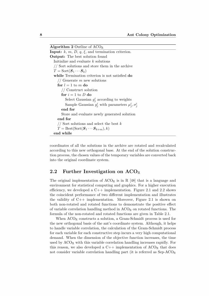
Algorithm 2 Outline of ACORInput: k, m, D, q, ξ, and termination criterion.Output: The best solution found
Initialize and evaluate k solutions// Sort solutions and store them in the archiveT = Sort(S1 · · ·Sk)while Termination criterion is not satisfied do// Generate m new solutionsfor l = 1 to m do// Construct solutionfor i = 1 to D doSelect Gaussian gij according to weightsSample Gaussian gij with parameters µij , σij
end forStore and evaluate newly generated solution
end for// Sort solutions and select the best kT = Best(Sort(S1 · · ·Sk+m), k)
end while
coordinates of all the solutions in the archive are rotated and recalculatedaccording to this new orthogonal base. At the end of the solution construc-tion process, the chosen values of the temporary variables are converted backinto the original coordinate system.
2.2 Further Investigation on ACOR
The original implementation of ACOR is in R [48] that is a language andenvironment for statistical computing and graphics. For a higher executionefficiency, we developed a C++ implementation. Figure 2.1 and 2.2 showsthe coincident performance of two different implementation and illustratesthe validity of C++ implementation. Moreover, Figure 2.1 is shown onboth non-rotated and rotated functions to demonstrate the positive effectof variable correlation handling method in ACOR on rotated functions. Theformula of the non-rotated and rotated functions are given in Table 2.1.
When ACOR constructs a solution, a Gram-Schmidt process is used forthe new orthogonal basis of the ant’s coordinate system. Although, it helpsto handle variable correlation, the calculation of the Gram-Schmidt processfor each variable for each constructive step incurs a very high computationaldemand. When the dimension of the objective function increases, the timeused by ACOR with this variable correlation handling increases rapidly. Forthis reason, we also developed a C++ implementation of ACOR that doesnot consider variable correlation handling part (it is referred as Sep-ACOR

2.2 Further Investigation on ACOR 9
Table 2.1: The formula of the non-rotated and rotated benchmark functionsfor Figure 2.1
The objective functionsellipsoid(~x) =
∑n
i=1(100i−1n−1 xi)2
rotatedellipsoid(~x) =∑n
i=1(100i−1n−1 zi)2
tablet(~x) = 104x12 +∑n
i=2 xi2
rotatedtablet(~x) = 104z12 +∑n
i=2 zi2
cigar(~x) = x12 + 104∑n
i=2 xi2
rotatedcigar(~x) = z12 + 104∑n
i=2 zi2
The definition of the variables~z = (~x)M, ~x ∈ (−3, 7)M is a random, normalized n-dimensional rotation matrix
throughout the rest of this thesis).To illustrate the execution time issue of ACOR, Figure 2.3 shows the av-
erage execution time of Sep-ACOR and ACOR in dependence of the numberof dimensions of the problem after 1000 evaluations. We fitted quadraticfunctions to the observed computation times. As seen from Figure 2.3, thefitted model for Sep-ACOR can be treated as linear due to the tiny coefficientfor the quadratic term. The execution time of ACOR scales quadraticallywith the dimensions of the testing problems. Taking the Rastrigin bench-mark function for example, the execution time of ACOR that correspondsto 40 dimensions after 1000 function evaluations is about 50 seconds. Sincethe time cost of each function evaluation is similar, ACOR need about 9hours for 1000 dimensional Rastrigin function every 1000 evaluations. Wecan predict that ACOR need about 5 years for 1000 dimensional rastriginfunction after 5000*D (D=1000) evaluations, which is the termination cri-terion for the large scale continuous optimization benchmark problems [46].Sep-ACOR only needs about 5 seconds and 7 hours for 1000 dimensionalrastrigin function after 1000 evaluations and 5000*D (D=1000) evaluations,respectively. With this variable correlation handling method, ACOR is dif-ficult and infeasible to apply to higher dimensional optimization problems.Therefore, Sep-ACOR is usually substituted for ACOR and it is extended toapply to many large scale optimization problems.
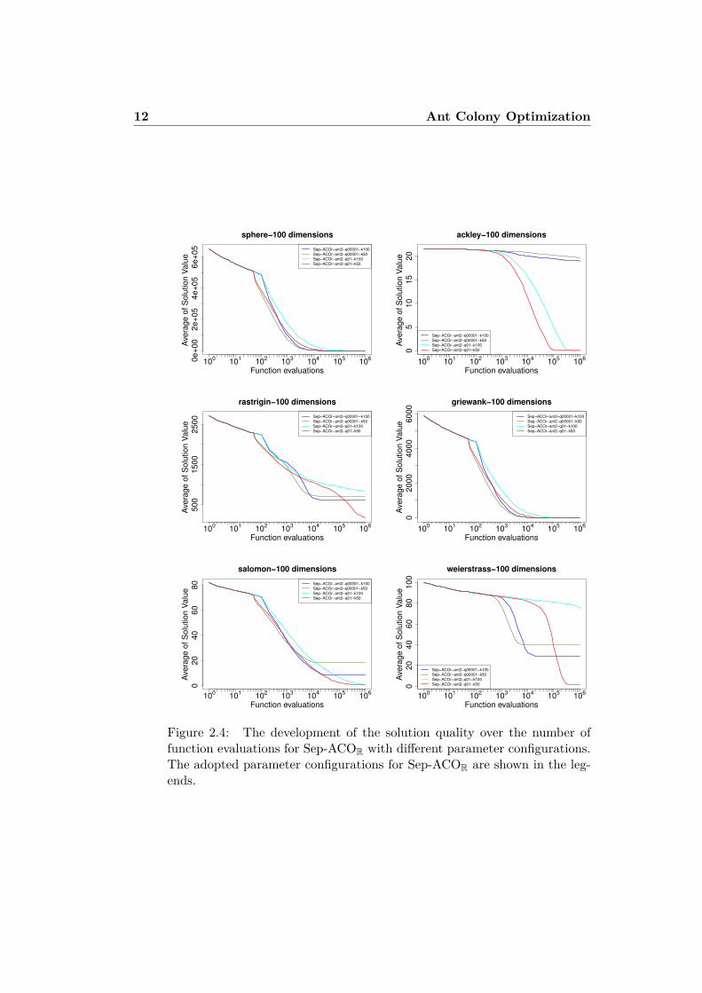
Figures 2.4 and 2.5 show the performance of Sep-ACOR with differentparameter configurations on selected 100 dimensional benchmark functions.We investigate the four different combinations of parameters q and k inthe ACOR algorithm (q ∈ (0.0001, 0.1), k ∈ (50, 100)), with the defaultparameters m = 2 and ξ = 0.85. Although Sep-ACOR has shown a goodperformance for continuous domains with certain parameter configurations,the gap with the-state-of-art continuous solvers is still considerable, whichis shown in the following Chapter 3. The different performances causedby different parameter configurations in Figures 2.4 and 2.5 indicate that aautomatic parameter tuning method may help to improve the performance

10 Ant Colony Optimization
of Sep-ACOR. In the following Chapter 3, an improved ACO algorithm ispresented.
AC
OrC
−d2
AC
OrR
−d2
AC
OrC
−d6
AC
OrR
−d6
AC
OrC
−d10
AC
OrR
−d10
AC
OrC
−d15
AC
OrR
−d15
0
10000
20000
30000
40000
50000
Nu
mb
ers
of
Eva
lua
tio
ns
ellipsoid, threshold= 1e−10
q=1e−04
mant=2
k=50
xi=0.85
AC
OrC
−d2
AC
OrR
−d2
AC
OrC
−d6
AC
OrR
−d6
AC
OrC
−d10
AC
OrR
−d10
AC
OrC
−d15
AC
OrR
−d15
0
10000
20000
30000
40000
50000
60000
Nu
mb
ers
of
Eva
lua
tio
ns
rotatedellipsoid, threshold= 1e−10
q=1e−04
mant=2
k=50
xi=0.85
AC
OrC
−d2
AC
OrR
−d2
AC
OrC
−d6
AC
OrR
−d6
AC
OrC
−d10
AC
OrR
−d10
AC
OrC
−d15
AC
OrR
−d15
1000
2000
3000
4000
5000
6000
Nu
mb
ers
of
Eva
lua
tio
ns
tablet, threshold= 1e−10
q=1e−04
mant=2
k=50
xi=0.85
AC
OrC
−d2
AC
OrR
−d2
AC
OrC
−d6
AC
OrR
−d6
AC
OrC
−d10
AC
OrR
−d10
AC
OrC
−d15
AC
OrR
−d15
1000
2000
3000
4000
5000
6000N
um
be
rs o
f E
valu
atio
ns
rotatedtablet, threshold= 1e−10
q=1e−04
mant=2
k=50
xi=0.85
AC
OrC
−d2
AC
OrR
−d2
AC
OrC
−d6
AC
OrR
−d6
AC
OrC
−d10
AC
OrR
−d10
AC
OrC
−d15
AC
OrR
−d15
0
2000
4000
6000
8000
10000
Nu
mb
ers
of
Eva
lua
tio
ns
cigar, threshold= 1e−10
q=1e−04
mant=2
k=50
xi=0.85
AC
OrC
−d2
AC
OrR
−d2
AC
OrC
−d6
AC
OrR
−d6
AC
OrC
−d10
AC
OrR
−d10
AC
OrC
−d15
AC
OrR
−d15
0
2000
4000
6000
8000
10000
Nu
mb
ers
of
Eva
lua
tio
ns
rotatedcigar, threshold= 1e−10
q=1e−04
mant=2
k=50
xi=0.85
Figure 2.1: The box-plot comparison between C++ and R implementationof ACOR on different dimensionality. ACOrC is the C++ implementationof ACOR and ACOrR is the original R implementation. The left box plotsare shown the numbers of function evaluations when achieving the thresholdof solution quality in non-rotated functions, on the right box-plots those ofrotated functions. We set the threshold of solution quality to 1e−10. Theadopted parameter configurations of ACOR are shown in the legends.

2.2 Further Investigation on ACOR 11
AC
OrC
−d
2
AC
OrR
−d
2
AC
OrC
−d
4
AC
OrR
−d
4
AC
OrC
−d
6
AC
OrR
−d
6
AC
OrC
−d
10
AC
OrR
−d
10
(96
%)
0
1000
2000
3000
4000
5000
Nu
mb
ers
of
eva
lua
tio
ns
ackley, threshold= 1e−04
q=0.1
mant=2
k=50
xi=0.85
AC
OrC
−d
2
AC
OrR
−d
2
AC
OrC
−d
4
AC
OrR
−d
4
AC
OrC
−d
6
AC
OrR
−d
6(8
8%
)
AC
OrC
−d
10
AC
OrR
−d
10
(92
%)
0
2000
4000
6000
8000
10000
Nu
mb
ers
of
eva
lua
tio
ns
rosenbrock, threshold= 1e−04
q=0.1
mant=2
k=50
xi=0.85
Figure 2.2: The box-plot comparison of C++ and R implementation ofACOR on different dimensionality of benchmark functions. ACOrC is theC++ implementation of ACOR and ACOrR is the original R implementa-tion. The box plots are shown the numbers of function evaluations whenachieving the threshold of solution quality. We set the threshold of solutionquality to 1e−04 for ackley and rosenbrock functions.
0 20 40 60 80 100
02
04
06
08
01
00
ellipsoid−1000 evaluations
dimensions
Ave
rag
e o
f exe
cu
tive
tim
e (
se
co
nd
s)
ACOr (0.036)x^2+(−0.084)x+(0.97)
Sep−ACOr (4e−08)x^2+(0.0019)x+(0.025)
0 20 40 60 80 100
02
04
06
08
01
00
sphere−1000 evaluations
dimensions
Ave
rag
e o
f exe
cu
tive
tim
e (
se
co
nd
s)
ACOr (0.028)x^2+(0.28)x+(−0.66)
Sep−ACOr (−1.4e−05)x^2+(0.0022)x+(0.022)
0 20 40 60 80 100
02
04
06
08
01
00
rosenbrock−1000 evaluations
dimensions
Ave
rag
e o
f exe
cu
tive
tim
e (
se
co
nd
s)
ACOr (0.047)x^2+(−0.41)x+(2.4)
Sep−ACOr (4.6e−06)x^2+(0.0014)x+(0.029)
0 20 40 60 80 100
02
04
06
08
01
00
rastrigin−1000 evaluations
dimensions
Ave
rag
e o
f exe
cu
tive
tim
e (
se
co
nd
s)
ACOr (0.033)x^2+(0.073)x+(0.25)
Sep−ACOr (3.9e−06)x^2+(0.0015)x+(0.029)
Figure 2.3: The fitted functions show the average time of Sep-ACOR andACOR after 1000 functions evaluations in dependence of the increasing di-mensionality. The fitted functions are modeled using the execution timeon 2, 3, 5, 7, 10, 15, 20, 25, 30, 35, 40 and 45 dimensions. The functionexpressions are shown in the legends.
12 Ant Colony Optimization
Function evaluations
Ave
rag
e o
f S
olu
tio
n V
alu
e
100
101
102
103
104
105
1060
e+
00
2e
+0
54
e+
05
6e
+0
5
sphere−100 dimensions
Sep−ACOr−ant2−q00001−k100
Sep−ACOr−ant2−q00001−k50
Sep−ACOr−ant2−q01−k100
Sep−ACOr−ant2−q01−k50
Function evaluations
Ave
rag
e o
f S
olu
tio
n V
alu
e
100
101
102
103
104
105
106
05
10
15
20
ackley−100 dimensions
Sep−ACOr−ant2−q00001−k100
Sep−ACOr−ant2−q00001−k50
Sep−ACOr−ant2−q01−k100
Sep−ACOr−ant2−q01−k50
Function evaluations
Ave
rag
e o
f S
olu
tio
n V
alu
e
100
101
102
103
104
105
106
50
01
50
02
50
0
rastrigin−100 dimensions
Sep−ACOr−ant2−q00001−k100
Sep−ACOr−ant2−q00001−k50
Sep−ACOr−ant2−q01−k100
Sep−ACOr−ant2−q01−k50
Function evaluations
Ave
rag
e o
f S
olu
tio
n V
alu
e
100
101
102
103
104
105
106
02
00
04
00
06
00
0griewank−100 dimensions
Sep−ACOr−ant2−q00001−k100
Sep−ACOr−ant2−q00001−k50
Sep−ACOr−ant2−q01−k100
Sep−ACOr−ant2−q01−k50
Function evaluations
Ave
rag
e o
f S
olu
tio
n V
alu
e
100
101
102
103
104
105
106
02
04
06
08
0
salomon−100 dimensions
Sep−ACOr−ant2−q00001−k100
Sep−ACOr−ant2−q00001−k50
Sep−ACOr−ant2−q01−k100
Sep−ACOr−ant2−q01−k50
Function evaluations
Ave
rag
e o
f S
olu
tio
n V
alu
e
100
101
102
103
104
105
106
02
04
06
08
01
00
weierstrass−100 dimensions
Sep−ACOr−ant2−q00001−k100
Sep−ACOr−ant2−q00001−k50
Sep−ACOr−ant2−q01−k100
Sep−ACOr−ant2−q01−k50
Figure 2.4: The development of the solution quality over the number offunction evaluations for Sep-ACOR with different parameter configurations.The adopted parameter configurations for Sep-ACOR are shown in the leg-ends.

2.2 Further Investigation on ACOR 13
an
t2−
q0
00
01
−k1
00
an
t2−
q0
00
01
−k5
0
an
t2−
q0
1−
k1
00
an
t2−
q0
1−
k5
0
1e−26
1e−20
1e−14
1e−08
1e−02
sphere−100 dimensions
So
lutio
n v
alu
e
an
t2−
q0
00
01
−k1
00
an
t2−
q0
00
01
−k5
0
an
t2−
q0
1−
k1
00
an
t2−
q0
1−
k5
0
1e−14
1e−10
1e−06
1e−02
ackley−100 dimensions
So
lutio
n v
alu
e
an
t2−
q0
00
01
−k1
00
an
t2−
q0
00
01
−k5
0
an
t2−
q0
1−
k1
00
an
t2−
q0
1−
k5
0
100
200
500
1000
rastrigin−100 dimensions
So
lutio
n v
alu
e
an
t2−
q0
00
01
−k1
00
an
t2−
q0
00
01
−k5
0
an
t2−
q0
1−
k1
00
an
t2−
q0
1−
k5
0
1e−20
1e−15
1e−10
1e−05
1e+00
griewank−100 dimensions
So
lutio
n v
alu
e
an
t2−
q0
00
01
−k1
00
an
t2−
q0
00
01
−k5
0
an
t2−
q0
1−
k1
00
an
t2−
q0
1−
k5
0
0.5
1.0
2.0
5.0
10.0
20.0
salomon−100 dimensions
So
lutio
n v
alu
e
an
t2−
q0
00
01
−k1
00
an
t2−
q0
00
01
−k5
0
an
t2−
q0
1−
k1
00
an
t2−
q0
1−
k5
0
1e−02
1e−01
1e+00
1e+01
1e+02
weierstrass−100 dimensions
So
lutio
n v
alu
e
Figure 2.5: The box-plots show the solution quality after 1E+06 functionevaluations for Sep-ACOR with different parameter configurations.


Chapter 3
An Incremental Ant ColonyAlgorithm with Local Search
As we have seen in Chapter 2, ACOR [83] and Sep-ACOR were further eval-uated and analyzed on selected benchmark functions. The main drawbacksare the high execution time cost for ACOR and the performance gap withthe-state-of-art continuous solvers, respectively. How to improve ACOR istherefore an important work. Recently, Leguizamón and Coello [57] pro-posed a variant of ACOR that performs better than the original ACOR onsix benchmark functions. However, the results obtained with Leguizamónand Coello’s variant are far from being competitive with the results obtainedby state-of-the-art continuous optimization algorithms recently featured ina special issue of the Soft Computing journal [64] (Throughout the restof this chapter, we will refer to this special issue as SOCO). The set ofalgorithms described in SOCO consists of differential evolution algorithms,memetic algorithms, particle swarm optimization algorithms and other typesof optimization algorithms [64]. In SOCO, the differential evolution algo-rithm (DE) [85], the covariance matrix adaptation evolution strategy withincreasing population size (G-CMA-ES) [7], and the real-coded CHC algo-rithm (CHC) [35] are used as the reference algorithms. It should be notedthat no ACO-based algorithms are featured in SOCO.
In this chapter, we propose an improved ACOR algorithm, called IACOR-LS, that is competitive with the state of the art in continuous optimization.We first present IACOR, which is an ACOR with an extra search diversi-fication mechanism that consists of a growing solution archive. Then, wehybridize IACOR with a local search procedure in order to enhance its searchintensification abilities. We experiment with three local search procedures:Powell’s conjugate directions set [76], Powell’s BOBYQA [77], and Lin-YuTseng’s Mtsls1 [93]. An automatic parameter tuning procedure, IteratedF-race [9, 13], is used for the configuration of the investigated algorithms.The best algorithm found after tuning, IACOR-Mtsls1, obtains results that

16 An Incremental Ant Colony Algorithm with Local Search
are as good as the best of the 16 algorithms featured in SOCO. To assessthe quality of IACOR-Mtsls1 and the best SOCO algorithms on problemsnot seen during their design phase, we compare their performance using anextended benchmark functions suite that includes functions from SOCO andthe special session on continuous optimization of the IEEE 2005 Congresson Evolutionary Computation (CEC 2005). The results show that IACOR-Mtsls1 can be considered to be a state-of-the-art continuous optimizationalgorithm.
3.1 The IACOR Algorithm
IACOR is an ACOR algorithm with a solution archive whose size increasesover time. This modification is based on the incremental social learningframework [70, 72]. A parameter Growth controls the rate at which thearchive grows. Fast growth rates encourage search diversification while slowones encourage intensification [70]. In IACOR the optimization process be-gins with a small archive, a parameter InitArchiveSize defines its size. A newsolution is added to it every Growth iterations until a maximum archive size,denoted by MaxArchiveSize, is reached. Each time a new solution is added,it is initialized using information from the best solution in the archive. First,a new solution Snew is generated completely at random. Then, it is movedtoward the best solution in the archive Sbest using
S′new = Snew + rand(0, 1)(Sbest − Snew) , (3.1)
where rand(0, 1) is a random number in the range [0, 1).IACOR also features a mechanism different from the one used in the
original ACOR for selecting the solution that guides the generation of newsolutions. The new procedure depends on a parameter p ∈ [0, 1], whichcontrols the probability of using only the best solution in the archive as aguiding solution. With a probability 1 − p, all the solutions in the archiveare used to generate new solutions. Once a guiding solution is selected,and a new one is generated (in exactly the same way as in ACOR), theyare compared. If the newly generated solution is better than the guidingsolution, it replaces it in the archive. This replacement strategy is differentfrom the one used in ACOR in which all the solutions in the archive and allthe newly generated ones compete.
We include an algorithm-level diversification mechanism for fighting stag-nation. The mechanism consists in restarting the algorithm and initializingthe new initial archive with the best-so-far solution. The restart criterion isthe number of consecutive iterations, MaxStagIter, with a relative solutionimprovement lower than a certain threshold.
3.2 IACOR with Local Search 17
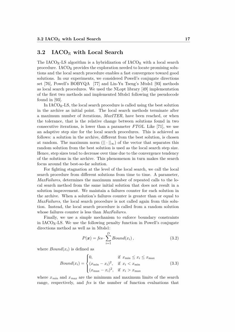
3.2 IACOR with Local SearchThe IACOR-LS algorithm is a hybridization of IACOR with a local searchprocedure. IACOR provides the exploration needed to locate promising solu-tions and the local search procedure enables a fast convergence toward goodsolutions. In our experiments, we considered Powell’s conjugate directionsset [76], Powell’s BOBYQA [77] and Lin-Yu Tseng’s Mtsls1 [93] methodsas local search procedures. We used the NLopt library [49] implementationof the first two methods and implemented Mtsls1 following the pseudocodefound in [93].
In IACOR-LS, the local search procedure is called using the best solutionin the archive as initial point. The local search methods terminate aftera maximum number of iterations, MaxITER, have been reached, or whenthe tolerance, that is the relative change between solutions found in twoconsecutive iterations, is lower than a parameter FTOL. Like [71], we usean adaptive step size for the local search procedures. This is achieved asfollows: a solution in the archive, different from the best solution, is chosenat random. The maximum norm (|| · ||∞) of the vector that separates thisrandom solution from the best solution is used as the local search step size.Hence, step sizes tend to decrease over time due to the convergence tendencyof the solutions in the archive. This phenomenon in turn makes the searchfocus around the best-so-far solution.
For fighting stagnation at the level of the local search, we call the localsearch procedure from different solutions from time to time. A parameter,MaxFailures, determines the maximum number of repeated calls to the lo-cal search method from the same initial solution that does not result in asolution improvement. We maintain a failures counter for each solution inthe archive. When a solution’s failures counter is greater than or equal toMaxFailures, the local search procedure is not called again from this solu-tion. Instead, the local search procedure is called from a random solutionwhose failures counter is less than MaxFailures.
Finally, we use a simple mechanism to enforce boundary constraintsin IACOR-LS. We use the following penalty function in Powell’s conjugatedirections method as well as in Mtsls1:
P (x) = fes ·D∑i=1
Bound(xi) , (3.2)
where Bound(xi) is defined as
Bound(xi) =
0, if xmin ≤ xi ≤ xmax
(xmin − xi)2, if xi < xmin
(xmax − xi)2, if xi > xmax
(3.3)
where xmin and xmax are the minimum and maximum limits of the searchrange, respectively, and fes is the number of function evaluations that

18 An Incremental Ant Colony Algorithm with Local Search
have been used so far. BOBYQA has its own mechanism for dealing withbound constraints. IACOR-LS is shown in Algorithm 3. The C++ imple-mentation of IACOR-LS is available in http://iridia.ulb.ac.be/supp/IridiaSupp2011-008/.
3.3 Experimental Study
Our study is carried out in two stages. First, we evaluate the performance ofACOR, IACOR-BOBYQA, IACOR-Powell and IACOR-Mtsls1 by comparingtheir performance with that of the 16 algorithms featured in SOCO. For thispurpose, we use the same 19 benchmark functions suite (functions labeledas fsoco∗). Second, we include 211 of the benchmark functions proposed forthe special session on continuous optimization organized for the IEEE 2005Congress on Evolutionary Computation (CEC 2005) [88] (functions labeledas fcec∗).
In the first stage of the study, we used the 50- and 100-dimensionalversions of the 19 SOCO functions. Functions fsoco1–fsoco6 were originallyproposed for the special session on large scale global optimization organizedfor the IEEE 2008 Congress on Evolutionary Computation (CEC 2008) [90].Functions fsoco7-fsoco11 were proposed at the ISDA 2009 Conference. Func-tions fsoco12-fsoco19 are hybrid functions that combine two functions belong-ing to fsoco1–fsoco11. The detailed description of these functions is availablein [46,64]. In the second stage of our study, the 19 SOCO and 21 CEC 2005functions on 50 dimensions were considered together. Some properties ofthe benchmark functions are listed in Table 3.1. The detailed description isavailable in [46,88].
We applied the termination conditions used for SOCO and CEC 2005were used, that is, the maximum number of function evaluations was 5000×D for the SOCO functions, and 10000×D for the CEC 2005 functions. Allthe investigated algorithms were run 25 times on each function. We reporterror values defined as f(x)−f(x∗), where x is a candidate solution and x∗
is the optimal solution. Error values lower than 10−14 (this value is referredto as 0-threshold) are approximated to 0. Our analysis is based on either thewhole solution quality distribution, or on the median and average errors.
3.3.1 Parameter Settings
We used Iterated F-race [9, 13] to automatically tune algorithm parame-ters. The 10-dimensional versions of the 19 SOCO functions were randomlysampled as training instances. A maximum of 50,000 algorithm runs wereused as tuning budget for ACOR, IACOR-BOBYQA, IACOR-Powell and
1From the original 25 functions, we decided to omit fcec1, fcec2, fcec6, and fcec9 becausethey are the same as fsoco1, fsoco3, fsoco4, fsoco8.

3.3 Experimental Study 19
Algorithm 3 Outline of IACOR-LSInput: : ξ, p, InitArchiveSize, Growth, MaxArchiveSize, FTOL, MaxITER, MaxFailures,
MaxStagIter, D and termination criterion.Output: The best solution foundk = InitArchiveSizeInitialize and evaluate k solutionswhile Termination criterion not satisfied do
// Local searchif FailedAttemptsbest < MaxFailures then
Invoke local search from Sbest with parameters FTOL and MaxITERelse
if FailedAttemptsrandom < MaxFailures thenInvoke local search from Srandom with parameters FTOL and MaxITER
end ifend ifif No solution improvement then
FailedAttemptsbest||random + +end if
// Generate new solutionsif rand(0,1)<p then
for i = 1 to D doSelect Gaussian gibestSample Gaussian gibest with parameters µibest, σ
ibest
end forif Newly generated solution is better than Sbest then
Substitute newly generated solution for Sbestend if
elsefor j = 1 to k do
for i = 1 to D doSelect Gaussian gijSample Gaussian gij with parameters µij , σij
end forif Newly generated solution is better than Sj then
Substitute newly generated solution for Sjend if
end forend if
// Archive Growthif current iterations are multiple of Growth & k < MaxArchiveSize then
Initialize new solution using Eq.3.1Add new solution to the archivek + +
end if// Restart Mechanismif # of iterations without improving Sbest = MaxStagIter then
Re-initialize T but keeping Sbestend if
end while

20 An Incremental Ant Colony Algorithm with Local Search
Table 3.1: Benchmark functionsID Name/Description Range Uni/Multi Sepa- Rotat-
[Xmin, Xmax]D modal rable edfsoco1 Shift.Sphere [-100,100]D U Y Nfsoco2 Shift.Schwefel 2.21 [-100,100]D U N Nfsoco3 Shift.Rosenbrock [-100,100]D M N Nfsoco4 Shift.Rastrigin [-5,5]D M Y Nfsoco5 Shift.Griewank [-600,600]D M N Nfsoco6 Shift.Ackley [-32,32]D M Y Nfsoco7 Shift.Schwefel 2.22 [-10,10]D U Y Nfsoco8 Shift.Schwefel 1.2 [-65.536,65.536]D U N Nfsoco9 Shift.Extended f10 [-100,100]D U N Nfsoco10 Shift.Bohachevsky [-15,15]D U N Nfsoco11 Shift.Schaffer [-100,100]D U N Nfsoco12 fsoco9 ⊕0.25 fsoco1 [-100,100]D M N Nfsoco13 fsoco9 ⊕0.25 fsoco3 [-100,100]D M N Nfsoco14 fsoco9 ⊕0.25 fsoco4 [-5,5]D M N Nfsoco15 fsoco10 ⊕0.25 fsoco7 [-10,10]D M N Nfsoco16 fsoco9 ⊕0.5 fsoco1 [-100,100]D M N Nfsoco17 fsoco9 ⊕0.75 fsoco3 [-100,100]D M N Nfsoco18 fsoco9 ⊕0.75 fsoco4 [-5,5]D M N Nfsoco19 fsoco10 ⊕0.75 fsoco7 [-10,10]D M N Nfcec3 Shift.Ro.Elliptic [-100,100]D U N Yfcec4 Shift.Schwefel 1.2 Noise [-100,100]D U N Nfcec5 Schwefel 2.6 Opt on Bound [-100,100]D U N Nfcec7 Shift.Ro.Griewank No Bound [0,600]D† M N Yfcec8 Shift.Ro.Ackley Opt on Bound [-32,32]D M N Yfcec10 Shift.Ro.Rastrigin [-5,5]D M N Yfcec11 Shift.Ro.Weierstrass [-0.5,0.5]D M N Yfcec12 Schwefel 2.13 [-π,π]D M N Nfcec13 Griewank plus Rosenbrock [-3,1]D M N Nfcec14 Shift.Ro.Exp.Scaffer [-100,100]D M N Yfcec15 Hybrid Composition [-5,5]D M N Nfcec16 Ro. Hybrid Composition [-5,5]D M N Yfcec17 Ro. Hybrid Composition [-5,5]D M N Yfcec18 Ro. Hybrid Composition [-5,5]D M N Yfcec19 Ro. Hybrid Composition [-5,5]D M N Yfcec20 Ro. Hybrid Composition [-5,5]D M N Yfcec21 Ro. Hybrid Composition [-5,5]D M N Yfcec22 Ro. Hybrid Composition [-5,5]D M N Yfcec23 Ro. Hybrid Composition [-5,5]D M N Yfcec24 Ro. Hybrid Composition [-5,5]D M N Yfcec25 Ro. Hybrid Composition [2,5]D† M N Y† denotes initialization range instead of bound constraints.
IACOR-Mtsls1. The number of function evaluations used in each run isequal to 50,000. The best set of parameters, for each algorithm found withthis process is given in Table 3.2. The only parameter that we set manuallywas MaxArchiveSize, which we set to 1,000.

3.3 Experimental Study 21
Table 3.2: Best parameter settings found through iterated F-Race forACOR, IACOR-BOBYQA, IACOR-Powell and IACOR-Mtsls1. The param-eter FTOL is first transformed as 10FTOL before using it in the algorithms.
ACORq ξ m k
0.04544 0.8259 10 85
IACOR-BOBYQA p ξ InitArchiveSize Growth FTOL MaxITER MaxFailures MaxStagIter0.6979 0.8643 4 1 -3.13 240 5 20
IACOR-Powellp ξ InitArchiveSize Growth FTOL MaxITER MaxFailures MaxStagIter
0.3586 0.9040 1 7 -1 20 6 8
IACOR-Mtsls1 p ξ InitArchiveSize Growth MaxITER MaxFailures MaxStagIter0.6475 0.7310 14 1 85 4 13
3.3.2 Experimental Results and Comparison
Figure 3.1 shows the distribution of median and average errors across the19 SOCO benchmark functions obtained with ACOR, IACOR-BOBYQA,IACOR-Powell, IACOR-Mtsls1 and the 16 algorithms featured in SOCO.2We marked with a + symbol those cases in which there is a statisticallysignificant difference at the 0.05 α-level with a Wilcoxon test with respectto IACOR-Mtsls1 (in favor of IACOR-Mtsls1). Also at the top of each plot,a count of the number of optima found by each algorithm (or an objectivefunction value lower than 10−14) is given.
In all cases, IACOR-Mtsls1 significantly outperforms ACOR, and is ingeneral more effective than IACOR-BOBYQA, and IACOR-Powell. IACOR-Mtsls1 is also competitive with the best algorithms in SOCO. If we considermedians only, IACOR-Mtsls1 significantly outperforms G-CMA-ES, CHC,DE, EVoPROpt, VXQR1, EM323, and RPSO-vm in both 50 and 100 di-mensions. In 100 dimensions, IACOR-Mtsls1 also significantly outperformsMA-SSW and GODE. Moreover, the median error of IACOR-Mtsls1 is be-low the 0-threshold 14 times out of the 19 possible of the SOCO benchmarkfunctions suite. Only MOS-DE matches such a performance.
If one considers mean values, the performance of IACOR-Mtsls1 de-grades slightly. This is an indication that IACOR-Mtsls1 still stagnateswith some low probability. However, IACOR-Mtsls1 still outperforms G-CMA-ES, CHC, GODE, EVoPROpt, RPSO-vm, and EM323. Even thoughIACOR-Mtsls1 does not significantly outperform DE and other algorithms,its performance is very competitive. The mean error of IACOR-Mtsls1 is be-low the 0-threshold 13 and 11 times in problems of 50 and 100 dimensions,respectively.
We note that although G-CMA-ES has difficulties in dealing with mul-timodal or unimodal shifted separable functions, such as fsoco4 , fsoco6 andfsoco7, G-CMA-ES showed impressive results on function fsoco8, which is ahyperellipsoid rotated in all directions. None of the other investigated al-
2For information about these 16 algorithms please go tohttp://sci2s.ugr.es/eamhco/CFP.php

22 An Incremental Ant Colony Algorithm with Local Search
gorithms can find the optimum of this function except G-CMA-ES. Thisresult is interesting considering that G-CMA-ES showed an impressive per-formance in the CEC 2005 special session on continuous optimization. Thisfact suggests that releasing details about the problems that will be usedto compare algorithms induces an undesired “overfitting” effect. In otherwords, authors may use the released problems to design algorithms thatperform well on them but that may perform poorly on another unknownset of problems. This motivated us to carry out the second stage of ourstudy, which consists in carrying out a more comprehensive comparisonthat includes G-CMA-ES and some of the best algorithms in SOCO. Forthis comparison, we use 40 benchmark functions as discussed above. FromSOCO, we include in our study IPSO-Powell given its good performance asshown in Figure 3.1. To discard the possibility that the local search pro-cedure is the main responsible for the obtained results, we also use Mtsls1with IPSO, thus generating IPSO-Mtsls1. In this second stage, IPSO-Powelland IPSO-Mtsls1 were tuned as described in Section 3.3.1.
Table 3.4 shows the median and average errors obtained by the comparedalgorithm on each of the 40 benchmark functions. Two facts can be noticedfrom these results. First, Mtsls1 seems to be indeed responsible for mostof the good performance of the algorithms that use it as a local searchprocedure. Regarding median results, the SOCO functions for which IPSO-Mtsls1 finds the optimum, IACOR-Mtsls1 does it as well. However, IACOR-Mtsls1 seems to be more robust given the fact that it finds more optima thanIPSO-Mtsls1 if functions from the CEC 2005 special session or mean valuesare considered. Second, G-CMA-ES finds more best results on the CEC2005 functions than on the SOCO functions. Overall, however, IACOR-Mtsls1 finds more best results than any of the compared algorithms.
Figure 3.2 shows correlation plots that illustrate the relative performancebetween IACOR-Mtsls1 and G-CMA-ES, IPSO-Powell and IPSO-Mtsls1.On the x-axis, the coordinates are the results obtained with IACOR-Mtsls1;on the y-axis, the coordinates are the results obtained with the other algo-rithms for each of the 40 functions. Thus, points that appear on the leftpart of the correlation plot correspond to functions for which IACOR-Mtsls1has better results than the other algorithm.
Table 3.3 shows a detailed comparison presented in form of (win, draw,lose) according to different properties of the 40 functions used. The two-sided p-values of Wilcoxon matched-pairs signed-ranks test of IACOR-Mtsls1with other algorithms across 40 functions are also presented. In general,IACOR-Mtsls1 performs better more often than all the other compared al-gorithms. IACOR-Mtsls1 wins more often against G-CMA-ES; however, G-CMA-ES performs clearly better than IACOR-Mtsls1 on rotated functions,which can be explained by the covariance matrix adaptation mechanism [42].

3.4 Conclusions 23
3.4 ConclusionsIn this chapter, we have introduced IACOR-LS, an ACOR algorithm withgrowing solution archive hybridized with a local search procedure. Threedifferent local search procedures, Powell’s conjugate directions set, Powell’sBOBYQA, and Mtsls1, were tested with IACOR-LS. Through automatictuning across 19 functions, IACOR-Mtsls1 proved to be superior to the othertwo variants.
The results of a comprehensive experimental comparison with 16 algo-rithms featured in a recent special issue of the Soft Computing journal showthat IACOR-Mtsls1 significantly outperforms the original ACOR and thatIACOR-Mtsls1 is competitive with the state of the art. We also conducteda second comparison that included 21 extra functions from the special ses-sion on continuous optimization of the IEEE 2005 Congress on Evolution-ary Computation. From this additional comparison we can conclude thatIACOR-Mtsls1 remains very competitive. It mainly shows slightly worseresults than G-CMA-ES on functions that are rotated w.r.t. the usual coor-dinate system. In fact, this is maybe not surprising as G-CMA-ES is the onlyalgorithm of the 20 compared ones that performs very well on these rotatedfunctions. In further work we may test ACOR in the version that includesthe mechanism for adjusting for rotated functions [83] to check whetherthese potential improvements transfer to IACOR-Mtsls1. Nevertheless, thevery good performance of IACOR-Mtsls1 on most of the Soft Computingbenchmark functions is a clear indication of the high potential hybrid ACOalgorithms have for this problem domain. In fact, IACOR-Mtsls1 is clearlycompetitive with state-of-the-art continuous optimizers.

24 An Incremental Ant Colony Algorithm with Local Search
DE
CHC
G−CMA−ES
SOUPDE
DE−D40−Mm
GODE
GaDE
jDElscop
SaDE−MMTS
MOS−DE
MA−SSW
RPSO−vm
IPSO−Powell
EvoPROpt
EM323
VXQR1
ACOr
IACOr−Bobyqa
IACOr−Powell
IACOr−Mtsls1
1e−
14
1e−
09
1e−
04
1e+
01
1e+
06
++
++
++
++
+O
ptim
a6
04
912
710
12
12
14
11
59
45
63
56
14
Median Errors of Fitness Value
DE
CHC
G−CMA−ES
SOUPDE
DE−D40−Mm
GODE
GaDE
jDElscop
SaDE−MMTS
MOS−DE
MA−SSW
RPSO−vm
IPSO−Powell
EvoPROpt
EM323
VXQR1
ACOr
IACOr−Bobyqa
IACOr−Powell
IACOr−Mtsls1
1e−
14
1e−
09
1e−
04
1e+
01
1e+
06
++
++
++
++
Optim
a6
02
89
69
12
12
14
94
50
56
25
613
Average Errors of Fitness Value
(a)50
dimen
sions
(b)50
dimen
sions
DE
CHC
G−CMA−ES
SOUPDE
DE−D40−Mm
GODE
GaDE
jDElscop
SaDE−MMTS
MOS−DE
MA−SSW
RPSO−vm
IPSO−Powell
EvoPROpt
EM323
VXQR1
ACOr
IACOr−Bobyqa
IACOr−Powell
IACOr−Mtsls1
1e−
14
1e−
09
1e−
04
1e+
01
1e+
06
++
++
++
++
++
+O
ptim
a6
03
911
611
12
12
14
10
58
36
63
56
14
Median Errors of Fitness Value
DE
CHC
G−CMA−ES
SOUPDE
DE−D40−Mm
GODE
GaDE
jDElscop
SaDE−MMTS
MOS−DE
MA−SSW
RPSO−vm
IPSO−Powell
EvoPROpt
EM323
VXQR1
ACOr
IACOr−Bobyqa
IACOr−Powell
IACOr−Mtsls1
1e−
14
1e−
09
1e−
04
1e+
01
1e+
06
++
++
++
++
+O
ptim
a6
02
89
69
10
12
13
84
50
45
25
611
Average Errors of Fitness Value(c)10
0dimen
sions
(d)10
0dimen
sions
Figure 3.1: The box-plots show the distribution of the median (left) and average(right) errors obtained on the 19 SOCO benchmark functions of 50 (top) and 100(bottom) dimensions. The results obtained with the three reference algorithmsin SOCO are shown on the left part of each plot. The results of 13 algorithmspublished in SOCO are shown in the middle part of each plot. The results obtainedwith ACOR, IACOR-BOBYQA, IACOR-Powell, and IACOR-Mtsls1 are shown onthe right part of each plot. The line at the bottom of each plot represents the 0-threshold (10−14). A + symbol on top of a box-plot denotes a statistically significantdifference at the 0.05 α-level detected with a Wilcoxon test between the resultsobtained with the indicated algorithm and those obtained with IACOR-Mtsls1.The absence of a symbol means that the difference is not significant with IACOR-Mtsls1. The numbers on top of a box-plot denotes the number of optima found bythe corresponding algorithm.

3.4 Conclusions 25
1e−14 1e−04 1e+061e
−1
41
e−
04
1e+
06
IACOr−mtsls1 (16 optima)
G−
CM
A−
ES
(5 o
ptim
a) IACOr−mtsls1
Win 21
Draw 3
Lose 16
Median Errors
1e−14 1e−04 1e+061e
−1
41
e−
04
1e+
06
IACOr−mtsls1 (14 optima)G
−C
MA
−E
S (
3 o
ptim
a) IACOr−mtsls1
Win 24
Draw 1
Lose 15
Average Errors
1e−14 1e−04 1e+061e
−14
1e−
04
1e+
06
IACOr−mtsls1 (16 optima)
Tuned IP
SO
−P
ow
ell
(10 o
ptim
a)
IACOr−mtsls1
Win 22
Draw 11
Lose 7
Median Errors
1e−14 1e−04 1e+061e
−14
1e−
04
1e+
06
IACOr−mtsls1 (14 optima)
Tu
ned IP
SO
−P
ow
ell
(6 o
ptim
a)
IACOr−mtsls1
Win 27
Draw 6
Lose 7
Average Errors
1e−14 1e−04 1e+061e−
14
1e−
04
1e+
06
IACOr−mtsls1 (16 optima)
Tun
ed IP
SO
−m
tsls
1 (
15 o
ptim
a)
IACOr−mtsls1
Win 16
Draw 17
Lose 7
Median Errors
1e−14 1e−04 1e+061e−
14
1e−
04
1e+
06
IACOr−mtsls1 (14 optima)
Tuned IP
SO
−m
tsls
1 (
8 o
ptim
a)
IACOr−mtsls1
Win 24
Draw 9
Lose 7
Average Errors
Figure 3.2: The correlation plot between IACOR-Mtsls1 and G-CMA-ES,IPSO-Powell and IPSO-Mtsls1 over 40 functions. Each point represents afunction. The points on the left part of correlation plot illustrate that onthose represented functions, IACOR-Mtsls1 obtains better results than theother algorithm.
26 An Incremental Ant Colony Algorithm with Local Search
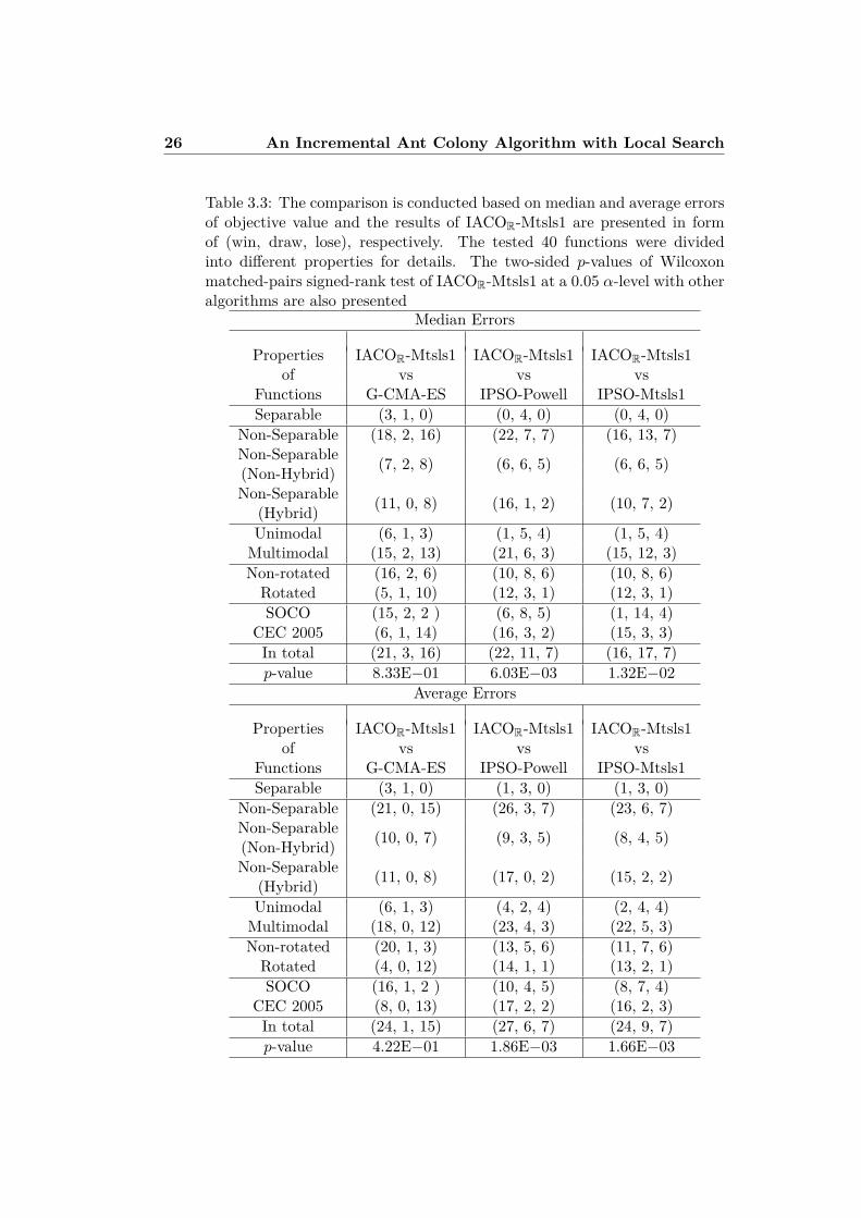
Table 3.3: The comparison is conducted based on median and average errorsof objective value and the results of IACOR-Mtsls1 are presented in formof (win, draw, lose), respectively. The tested 40 functions were dividedinto different properties for details. The two-sided p-values of Wilcoxonmatched-pairs signed-rank test of IACOR-Mtsls1 at a 0.05 α-level with otheralgorithms are also presented
Median Errors
Properties IACOR-Mtsls1 IACOR-Mtsls1 IACOR-Mtsls1of vs vs vs
Functions G-CMA-ES IPSO-Powell IPSO-Mtsls1Separable (3, 1, 0) (0, 4, 0) (0, 4, 0)
Non-Separable (18, 2, 16) (22, 7, 7) (16, 13, 7)Non-Separable (7, 2, 8) (6, 6, 5) (6, 6, 5)(Non-Hybrid)Non-Separable (11, 0, 8) (16, 1, 2) (10, 7, 2)(Hybrid)
Unimodal (6, 1, 3) (1, 5, 4) (1, 5, 4)Multimodal (15, 2, 13) (21, 6, 3) (15, 12, 3)Non-rotated (16, 2, 6) (10, 8, 6) (10, 8, 6)Rotated (5, 1, 10) (12, 3, 1) (12, 3, 1)SOCO (15, 2, 2 ) (6, 8, 5) (1, 14, 4)
CEC 2005 (6, 1, 14) (16, 3, 2) (15, 3, 3)In total (21, 3, 16) (22, 11, 7) (16, 17, 7)p-value 8.33E−01 6.03E−03 1.32E−02
Average Errors
Properties IACOR-Mtsls1 IACOR-Mtsls1 IACOR-Mtsls1of vs vs vs
Functions G-CMA-ES IPSO-Powell IPSO-Mtsls1Separable (3, 1, 0) (1, 3, 0) (1, 3, 0)
Non-Separable (21, 0, 15) (26, 3, 7) (23, 6, 7)Non-Separable (10, 0, 7) (9, 3, 5) (8, 4, 5)(Non-Hybrid)Non-Separable (11, 0, 8) (17, 0, 2) (15, 2, 2)(Hybrid)
Unimodal (6, 1, 3) (4, 2, 4) (2, 4, 4)Multimodal (18, 0, 12) (23, 4, 3) (22, 5, 3)Non-rotated (20, 1, 3) (13, 5, 6) (11, 7, 6)Rotated (4, 0, 12) (14, 1, 1) (13, 2, 1)SOCO (16, 1, 2 ) (10, 4, 5) (8, 7, 4)
CEC 2005 (8, 0, 13) (17, 2, 2) (16, 2, 3)In total (24, 1, 15) (27, 6, 7) (24, 9, 7)p-value 4.22E−01 1.86E−03 1.66E−03

3.4 Conclusions 27
Table 3.4: The median and average errors of objective function values ob-tained with G-CMA-ES, IPSO-Powell, IPSO-Mtsls1, and IACOR-Mtsls1 on40 functions with D = 50. The lowest values were highlighted in boldface.The values below 10−14 are approximated to 0. The results of fcec1, fcec2,fcec6, fcec9 are not presented to avoid repeated test on the similar functionssuch as fsoco1, fsoco3, fsoco4, fsoco8. At the bottom of the table, we reportthe number of times an algorithm found the lowest error.
Median errors Mean errorsFunctionG-CMA-ESIPSO-PowellIPSO-Mtsls1IACOR-Mtsls1FunctionG-CMA-ESIPSO-PowellIPSO-Mtsls1IACOR-Mtsls1fsoco1 0.00E+00 0.00E+00 0.00E+00 0.00E+00 fsoco1 0.00E+00 0.00E+00 0.00E+00 0.00E+00fsoco2 2.64E−11 1.42E−14 4.12E−13 4.41E−13 fsoco2 2.75E−11 2.56E−14 4.80E−13 5.50E−13fsoco3 0.00E+00 0.00E+00 6.38E+00 4.83E+01 fsoco3 7.97E−01 0.00E+00 7.29E+01 8.17E+01fsoco4 1.08E+02 0.00E+00 0.00E+00 0.00E+00 fsoco4 1.05E+02 0.00E+00 1.31E+00 0.00E+00fsoco5 0.00E+00 0.00E+00 0.00E+00 0.00E+00 fsoco5 2.96E−04 6.72E−03 5.92E−04 0.00E+00fsoco6 2.11E+01 0.00E+00 0.00E+00 0.00E+00 fsoco6 2.09E+01 0.00E+00 0.00E+00 0.00E+00fsoco7 7.67E−11 0.00E+00 0.00E+00 0.00E+00 fsoco7 1.01E−10 4.98E−12 0.00E+00 0.00E+00fsoco8 0.00E+00 1.75E−09 2.80E−10 2.66E−05 fsoco8 0.00E+00 4.78E−09 4.29E−10 2.94E−05fsoco9 1.61E+01 0.00E+00 0.00E+00 0.00E+00 fsoco9 1.66E+01 4.95E−06 0.00E+00 0.00E+00fsoco10 6.71E+00 0.00E+00 0.00E+00 0.00E+00 fsoco10 6.81E+00 0.00E+00 0.00E+00 0.00E+00fsoco11 2.83E+01 0.00E+00 0.00E+00 0.00E+00 fsoco11 3.01E+01 8.19E−02 7.74E−02 0.00E+00fsoco12 1.87E+02 1.02E−12 0.00E+00 0.00E+00 fsoco12 1.88E+02 1.17E−11 7.27E−03 0.00E+00fsoco13 1.97E+02 2.00E−10 5.39E−01 6.79E−01 fsoco13 1.97E+02 2.65E−10 2.75E+00 3.03E+00fsoco14 1.05E+02 1.77E−12 0.00E+00 0.00E+00 fsoco14 1.09E+02 1.18E+00 5.26E−01 3.04E−01fsoco15 8.12E−04 1.07E−11 0.00E+00 0.00E+00 fsoco15 9.79E−04 2.62E−11 0.00E+00 0.00E+00fsoco16 4.22E+02 3.08E−12 0.00E+00 0.00E+00 fsoco16 4.27E+02 2.80E+00 2.46E+00 0.00E+00fsoco17 6.71E+02 4.35E−08 1.47E+01 6.50E+00 fsoco17 6.89E+02 3.10E+00 7.27E+01 6.19E+01fsoco18 1.27E+02 8.06E−12 0.00E+00 0.00E+00 fsoco18 1.31E+02 1.24E+00 1.68E+00 0.00E+00fsoco19 4.03E+00 1.83E−12 0.00E+00 0.00E+00 fsoco19 4.76E+00 1.19E−11 0.00E+00 0.00E+00fcec3 0.00E+00 8.72E+03 1.59E+04 8.40E+05 fcec3 0.00E+00 1.24E+04 1.62E+04 9.66E+05fcec4 4.27E+05 2.45E+02 3.88E+03 5.93E+01 fcec4 4.68E+05 2.90E+02 4.13E+03 7.32E+01fcec5 5.70E−01 4.87E−07 7.28E−11 9.44E+00 fcec5 2.85E+00 4.92E−06 2.32E−10 9.98E+00fcec7 3.85E−14 0.00E+00 0.00E+00 0.00E+00 fcec7 5.32E−14 0.00E+00 0.00E+00 0.00E+00fcec8 2.00E+01 2.00E+01 2.00E+01 2.00E+01 fcec8 2.01E+01 2.00E+01 2.00E+01 2.00E+01fcec10 9.97E−01 8.96E+02 8.92E+02 2.69E+02 fcec10 1.72E+00 9.13E+02 8.76E+02 2.75E+02fcec11 1.21E+00 6.90E+01 6.64E+01 5.97E+01 fcec11 1.17E+01 6.82E+01 6.63E+01 5.90E+01fcec12 2.36E+03 5.19E+04 3.68E+04 1.37E+04 fcec12 2.27E+05 5.68E+04 5.86E+04 1.98E+04fcec13 4.71E+00 3.02E+00 3.24E+00 2.14E+00 fcec13 4.59E+00 3.18E+00 3.32E+00 2.13E+00fcec14 2.30E+01 2.35E+01 2.36E+01 2.33E+01 fcec14 2.29E+01 2.34E+01 2.35E+01 2.31E+01fcec15 2.00E+02 2.00E+02 2.00E+02 0.00E+00 fcec15 2.04E+02 1.82E+02 2.06E+02 9.20E+01fcec16 2.15E+01 4.97E+02 4.10E+02 3.00E+02 fcec16 3.09E+01 5.22E+02 4.80E+02 3.06E+02fcec17 1.61E+02 4.54E+02 4.11E+02 4.37E+02 fcec17 2.34E+02 4.46E+02 4.17E+02 4.43E+02fcec18 9.13E+02 1.22E+03 1.21E+03 9.84E+02 fcec18 9.13E+02 1.18E+03 1.19E+03 9.99E+02fcec19 9.12E+02 1.23E+03 1.19E+03 9.93E+02 fcec19 9.12E+02 1.22E+03 1.18E+03 1.01E+03fcec20 9.12E+02 1.22E+03 1.19E+03 9.93E+02 fcec20 9.12E+02 1.20E+03 1.18E+03 9.89E+02fcec21 1.00E+03 1.19E+03 1.03E+03 5.00E+02 fcec21 1.00E+03 9.86E+02 8.59E+02 5.53E+02fcec22 8.03E+02 1.43E+03 1.45E+03 1.13E+03 fcec22 8.05E+02 1.45E+03 1.47E+03 1.14E+03fcec23 1.01E+03 5.39E+02 5.39E+02 5.39E+02 fcec23 1.01E+03 7.66E+02 6.13E+02 5.67E+02fcec24 9.86E+02 1.31E+03 1.30E+03 1.11E+03 fcec24 9.55E+02 1.29E+03 1.30E+03 1.10E+03fcec25 2.15E+02 1.50E+03 1.59E+03 9.38E+02 fcec25 2.15E+02 1.18E+03 1.50E+03 8.89E+02
# of best 18 15 18 21 # of best 14 10 10 22


Chapter 4
Ant Colony Optimization forMixed Variable Problems
Recently, many real world problems are modeled using a mixed types of de-cision variables. A common example is a mixture of discrete variables andcontinuous variables. The former usually involve ordering characteristics,categorical characteristic or both of them. Due to the practical relevance ofsuch problems, many mixed-variable optimization algorithms have been pro-posed, mainly based on Genetic Algorithms [38], Differential Evolution [85],Particle Swarm Optimization [51] and Pattern Search [92]. In many cases,the discrete variables are tackled as ordered through a continuous relaxationapproach [23,40,55,56,79,94] based on continuous optimization algorithms.In many other cases, the discrete variables are tackled as categorical througha native mixed-variable optimization approach [6, 22, 74] that simultaneousand directly handles both discrete and continuous variables without relax-ation. However, It is mentioned that the available approaches are indiffer-ent with either categorical or ordering characteristics of discrete variables.Therefore, there is lack of a generic algorithm which allows to declare eachvariable of the considered problem as continuous, ordered discrete or cate-gorical discrete.
While ant colony optimization (ACO) was originally introduced to solvediscrete optimization problems [24, 25, 87], its adaptation to solve continu-ous optimization problems enjoys an increasing attention [10,32,67] as alsodiscussed in the previous chapter. However, few ACO extensions are appliedto mixed-variable optimization problems.
In this chapter, we present ACOMV, an ACOR extension for mixed-variable optimization problems. ACOMV integrates a component of acontinuous relaxation approach (ACOMV-o) and a component of a nativemixed-variable optimization approach (ACOMV-c), as well as ACOR and al-lows to declare each variable of the mixed variable optimization problems ascontinuous, ordered discrete or categorical discrete. We also propose a new

30 Ant Colony Optimization for Mixed Variable Problems
set of artificial mixed-variable benchmark functions and their constructivemethods, thereby providing a flexibly controlled environment for investigat-ing the performance and training parameters of mixed-variable optimizationalgorithms. We automatically tune the parameters of ACOMV by the it-erated F-race method [9, 13]. Then, we not only evaluate the performanceof ACOMV on benchmark functions, but also compare the performance ofACOMV on 4 classes of 8 mixed-variables engineering optimization prob-lems with the results from literature. ACOMV has efficiently found all thebest-so-far solution including two new best solution. ACOMV obtains 100%success rate in 7 problems. In 5 of those 7 problems, ACOMV requires thesmallest number of function evaluations. To sum up, ACOMV has the bestperformance on mixed-variables engineering optimization problems from theliterature.
4.1 Mixed-variable Optimization Problems
A model for a mixed-variable optimization problem (MVOP) may be for-mally defined as follows:
Definition A model R = (S,Ω, f) of a MVOP consists of
• a search space S defined over a finite set of both discrete and continuousdecision variables and a set Ω of constraints among the variables;
• an objective function f : S→ R+0 to be minimized.
The search space S is defined as follows: Given is a set of n = d + rvariables Xi, i = 1, . . . , n, of which d are discrete with valuesvji ∈ Di = v1
i , . . . , v|Di|i , and r are continuous with possible values
vi ∈ Di ⊆ R. Specifically, the discrete search space is expanded to be definedas a set of d = o+ c variables, of which o are ordered and c are categoricaldiscrete variables, respectively. A solution s ∈ S is a complete assignment inwhich each decision variable has a value assigned. A solution that satisfiesall constraints in the set Ω is a feasible solution of the given MVOP. If theset Ω is empty, R is called an unconstrained problem model, otherwise itis said to be constrained. A solution s∗ ⊆ S is called a global optimum ifand only if: f(s∗) ≤ f(s) ∀s∈S. The set of all globally optimal solutionsis denoted by S∗ ⊆ S. Solving a MVOP requires finding at least one s∗ ⊆ S∗.
The methods proposed in the literature to tackle MVOPs may be dividedinto three groups.
The first group is based on a two-partition approach, in which the mixedvariables are decomposed into two partitions, one involving the continuousvariables and the other involving the discrete variables. Variables of one

4.1 Mixed-variable Optimization Problems 31
partition are optimized separately for fixed values of the variable of theother partition [78]. The approach usually leads to a large number of ob-jective function evaluations [84] and the dependency of variables may leadto a sub-optimal solution. More promising are the other two groups. Thesecond group is a continuous relaxation approach. Discrete variables arerelaxed to continuous variables, but are repaired when evaluating the ob-jective function. The repair mechanism is used to return a discrete variablein each iteration. The simplest repair mechanisms are by truncation androunding [40, 55]. The performance depends on the continuous solvers andthe repair mechanisms. The third group is a native mixed-variable opti-mization approach that simultaneously and directly handles both discreteand continuous variables without relaxation. It is indifferent to the orderingcharacter of the discrete variables. Genetic adaptive search, pattern search,and mixed bayesian optimization are among the approaches that have beenproposed in [6, 22,74].
A particular class of MVOPs is known as mixed variable programming(MVP) problems [6]. They are characterized by a combination of continuousand categorical variables. The latter are discrete variables that take theirvalues from a set of categories [4]. Categorical variables often identify non-numeric elements of an unordered set (colors, shapes or type of materials)and characterize the structure of problems [65]. Therefore, the discretenessof categorical variables must be satisfied at every iteration when consideringpotential iterative solution approaches [2].
However, MVP problems are not considered about the ordering nature ofdiscrete variables, and the solvers for MVP problems are almost based on anative mixed-variable optimization approach. Therefore, Those solvers maynot efficiently handle highly ordered variables owing to the lack of continuousrelaxations.
In another aspect, [1] claims modeling without categorical variables sothat continuous relaxations may be used to handle categorical variables. Butthe performance of continuous relaxations may decline with an increasingnumber of categories. Therefore, a possible more rigorous way of classifyingMVOPs is to consider whether the discrete variables are ordered or categor-ical ones, since they are both important characters for discrete variables.
Whereas, researchers often take one specific group of approaches to de-velop mixed-variable optimization algorithms and test on MVOPs with onespecific type of discrete variables, finally obtain reasonable good results,rather than investigating those algorithms on MVOPs with other types ofdiscrete variables. Therefore, there is lack of rigorous comparisons betweencontinuous relaxation approach and native mixed-variable optimization ap-proach, let alone taking the advantage of the strategies of the both ap-proaches to improve algorithms performance on more general and variousMVOPs. However, in our study, we have done those work in Section 4.4 andSection 4.6.

32 Ant Colony Optimization for Mixed Variable Problems
4.2 ACOMV Heuristics for Mixed-VariableOptimization Problems
We start by describing the ACOMV heuristic framework, and then, we de-scribe the probabilistic solution construction for continuous variables, or-dered discrete variables and categorical variables, respectively.
4.2.1 ACOMV framework
The basic flow of the ACOMV algorithm is as follows. As a first step, thesolution archive is initialized. Then, at each iteration a number of solutionsis probabilistically constructed by the ants. These solutions may be im-proved by any improvement mechanism (for example, local search or gradi-ent techniques). Finally, the solution archive is updated with the generatedsolutions. In the following we outline the archive structure, the initializationand the update of the archive in more details.
ACOMV keeps a history of its search process by storing solutions in asolution archive T of dimension |T | = k. Given an n-dimensional MVOPand k solutions, ACOMV stores the values of the solutions’ n variables andthe solutions’ objective function values in T . The value of the i-th variableof the j-th solution is in the following denoted by sij . Figure 4.1 shows thestructure of the solution archive. It is divided into three groups of columns,one for categorical variables, one for ordered discrete variables and one forcontinuous variables. ACOMV-c and ACOMV-o handle categorical variablesand ordered discrete variables, respectively, while ACOR handles continuousvariables.
Before the start of the algorithm, the archive is initialized with k randomsolutions. At each algorithm iteration, first, a set ofm solutions is generatedby the ants and added to those in T . From this set of k +m solutions, them worst ones are removed. The remaining k solutions are sorted accordingto their quality (i.e., the value of the objective function) and stored in thenew T . In this way, the search process is biased towards the best solutionsfound during the search. The solutions in the archive are always kept sortedbased on their quality, so that the best solution is on top. An outline of theACOMV algorithm is given in Algorithm 4.
4.2.2 Probabilistic Solution Construction for ContinuousVariables
Continuous variables are handled by ACOR [83], which has been furtherexplained in Chapter 2.1.

4.2 ACOMV Heuristics for Mixed-Variable Optimization Problems 33
Figure 4.1: The structure of the solution archive of ACOMV. The solutionsin the archive are sorted according to their quality, i.e., the value of theobjective function f(si)), hence, the position of a solution in the archivealways corresponds to its rank.
4.2.3 Probabilistic Solution Construction for OrderedDiscrete Variables
If ordered discrete variables are defined, a component of the continuousrelaxation approach, ACOMV-o, is used. The natural ordering of the valuesfor these variables may have little to do with their actual numerical values(and they may even not have numerical values, e.g., x ∈ small, big,huge).Hence, instead of operating on the actual values of the ordered discretevariables, ACOMV-o operates on their indexes. The values of the indexesfor the new solutions are generated as real numbers, as it is the case for thecontinuous variables. However, before the objective function is evaluated,the continuous values are rounded to the nearest valid index, and the valueat that index is then used for the objective function evaluation. At thealgorithm level, ordered discrete variables are transformed into continuousvariables for probabilistically constructing solution.

34 Ant Colony Optimization for Mixed Variable Problems
Algorithm 4 Outline of ACOMVInitialize decision variables
Categorical varables → array(C)Ordering discrete varables → array(O)Continuous varables → array(R)
// Initialize pheromonesInitialize solution archive(T ) of size Kwhile termination criterion not satisfied do// ConstructAntSolutionfor n = 1 to Nants do// ConstructSolution(S1 · · ·SNants)Probabilistic Solution Construction for ACOMV-cProbabilistic Solution Construction for ACOMV-oProbabilistic Solution Construction for ACOR
end forTnew= Firstk ⇐ Rank(S(T ) ∪ S1 · · ·SNants)// Update pheromonesUpdate solution achive(T )
end while
4.2.4 Probabilistic Solution Construction for CategoricalVariables
While ordered discrete variables are relaxed and treated in the originalACOR, categorical variables are treated differently in a component of thenative discrete optimization approach, ACOMV-c, as for this type of vari-ables there is no pre-defined ordering. The pheromone representation (i.e.,the solution archive) as well as the general flow of ACOMV does not change.Hence, we focus here on presenting how the discrete variables are handledwithout the ordered information in the domain. The values for these vari-ables are generated with a different method—one that is closer to the regularcombinatorial ACO.
In standard ACO (see [26]), solutions are constructed from solution com-ponents using a probabilistic rule based on the pheromone values. Dif-ferently, in ACOMV there are no static pheromone values, but a solutionarchive. As in standard ACO, in ACOMV-c, the construction of solutionsfor categorical variables is done by choosing the components, that are, thevalues for each of the categorical decision variables. However, since thepheromone model of standard ACO are replaced by the solution archive,the probabilistic solution construction rule is modified as follows.
Similarly to the case of continuous variables, each ant constructs thecategorical discrete part of the solution incrementally. For each categoricalvariable i, each ant chooses probabilistically one of ci available values vil ∈

4.2 ACOMV Heuristics for Mixed-Variable Optimization Problems 350
.00
0.0
40
.08
0.1
2
ranks
pro
ba
bili
ty
1 2 3 4 5 6 7 8 9
f c d e b
0.0
00
.10
0.2
00
.30
Final Probabilities
categories
pro
ba
bili
ty
a b c d e f g
Figure 4.2: Calculating probabilities of choosing different categorical valuesfor a given decision variable. First, the initial probabilities are generatedusing a normal distribution and based on the best ranked solution that usesgiven value (left plot, dashed bars). Then, they are divided by the numberof solutions using this value (left plot, solid bars), and finally a fixed valueis added (right plot, dotted bars) in order to increase the probability ofchoosing those values, which are currently not used. The final probabilitiesare presented on the right plot, as solid bars.
Di = vi1, ..., vici. The probability of choosing the l-th value is given by:
oil = wl∑cr=1wr
, (4.1)
where wl is the weight associated with the l-th available value. It is calcu-lated based on the weights ω and some additional parameters:
wl = ωjluil
+ q
η. (4.2)
The final weight wl is hence a sum of two components. The weight ωjl iscalculated according to Equation 2.2, where the jl is the index of the highestquality solution that uses value vil for the i-th categorical variable. In turn,uil is the number of solutions using value vil for the i-th categorical variablein the archive. Therefore, the more popular the value vil is, the lower is itsfinal weight.
The second component is a fixed value (i.e., it does not depend on thevalue vil chosen): η is the number of values from the ci available ones thatare unused by the solutions in the archive, and q is the same parameter ofthe algorithm that was used in Equation 2.2.

36 Ant Colony Optimization for Mixed Variable Problems
The graphical representation of how the first component ωjluil
is calculatedis presented on the left plot of Figure 4.2. The dashed bars indicate thevalues of the weights ωjl obtained for the best solutions using the availablevalues. 1 The solid bars represent the weights ωjl divided by the respectivenumber of solutions uil that use values vil . It is shown for the available setof categorical values used, vil ∈ a,b, c,d, e, f, g in this example.
Some of the available categorical values vl may be unused for a giveni-th decision variable in all the solutions in the archive. Hence, their initialweight is zero. In order to enhance exploration and to prevent prematureconvergence, in such a case, the final weights w are further modified byadding to all of them the second component. Its value depends on theparameter q and on the number of unused categorical values ηi, as shown inEquation 4.2.
The right plot in Figure 4.2 presents the normalized final probabilities foran example in which the solution archive has size k = 10, and where the setof categorical values is a,b, c,d, e, f, g, with values a and g unused bythe current decision variable. The dotted bars show the value of q/η addedto all the solutions, and the solid bars show the final resulting probabilitiesassociated with each of the available categories. These probabilities are thenused to generate the value of the i-th decision variable for the new solutions.
4.2.5 Auxiliary Explanations of ACOMV
The following are some auxiliary explanations of ACOMV. ACO algorithmsin general do not exploit correlation information between different deci-sion variables (or components). In ACOMV, due to the specific way thepheromone is represented (i.e., as the solution archive), it is in fact possibleto take into account the correlation between the decision variables. A non-deterministic adaptive method is presented in [83], which will take effecton rotated benchmark functions proposed in Section 4.3, and also handlevariable dependency of engineering problem in Section 4.6.
For simplification of ACOMV, The uniform random sampling in therange of decision variables is used for initial solution archive. For fight-ing stagnation, a simple restart strategy consists in restarting the algorithmbut keeping the best-so-far solution in archive. The restart criterion is thenumber of iterations of ants updating the archive with a relative solutionimprovement lower than a certain threshold ε. ACOMV is implemented inC++.
1If a given value is not used, the associated index is indefinite, and thus its initialweight is zero.

4.3 Artificial Mixed-variable Benchmark Functions 37
4.3 Artificial Mixed-variable BenchmarkFunctions
The mixed-variable benchmark problems found in the literature oftenoriginate from the mechanical engineering field, which can not be easilyparametrized and flexibly manipulated for investigating the performance ofmixed-variable optimization algorithms.
In this section, we propose a set of new, artificial mixed-variable bench-mark functions for a sufficiently controlled environment for the investigationof the performance and the automatic parameter tuning of algorithms. Ourproposed artificial mixed-variable benchmark functions are defined in Ta-ble 4.1. The expressions of objective functions originate from some typicalcontinuous functions in IEEE CEC 2005. The decision variables consist ofdiscrete and continuous variables. n is the number of dimensions includingdiscrete variables and continuous variables and M is a random, normalizedn-dimensional rotation matrix. The continuous variables’ global optima areshifted to avoid a bias of population based methods towards the center ofthe search space [34]. It allows 3 settings for discrete variables, one involv-ing ordered discrete variables, one involving categorical variables and oneinvolving mixed ordered discrete and categorical variables.
In order to make it easier to understand and visualize the benchmarkfunctions, we use the two dimensional, not shifted, randomly rotated Ellip-soid mixed-variable functions as an example to illustrate the principle of howto construct artificial mixed-variable benchmark functions. Equation 4.3 israndomly rotated Ellipsoid continuous function.
fEL(~x) =n∑i=1
(βi−1n−1 zi)2,
~x ∈ (−3, 7)n,~z = M~x,
(4.3)
In order to transform this continuous function into a mixed-variable one,we have divided the continuous domain of variable x1 ∈ (−3, 7) into a setof discrete values, T = θ1, θ2, ..., θt : θi ∈ (−3, 7). This results in thefollowing mixed-variable test function:
fELMV(~x) = z2
1 + β · z22 ,
x1 ∈ T,x2 ∈ (−3, 7),~z = M~x.
(4.4)
The set T is created by choosing t uniformly spaced values from the originaldomain (−3, 7) in such a way that ∃i=1,...,t θi = 0. This way, it is alwayspossible to find the optimum value fELMV
(0, 0) = 0, regardless of the chosent discrete values.
In the following, we will explain the first two setups of discrete variablesto simulate each benchmark function, respectively: (i) with ordered discretevariables, and (ii) with categorical variables. In the first setup, the discrete

38 Ant Colony Optimization for Mixed Variable Problems
Table 4.1: Artificial mixed-variable benchmark functions
The objective functionsfEllipsoidMV
(~x) = ∑ni=1(β
i−1n−1 zi)2,
fAckleyMV(~x) = −20e−0.2
√1n
∑n
i=1(z2i ) − e
1n
∑n
i=1(cos(2πzi)) + 20 + e,
fRastriginMV(~x) = 10n+∑n
i=1(z2i − 10 cos(2πz2
i )),fRosenbrockMV
(~x) = ∑n−1i=1 [100(zi+1 − z2
i )2 + (zi − 1)2],fSphereMV
(~x) = ∑ni=1 z
2i ,
fGriewankMV(~x) = 1
4000∑ni=1 z
2i −
∏ni=1 cos( zi√
i) + 1,
The definition of mixed variables~xd ∈ T,T = θ1, θ2, ..., θt : θi ∈ (MinRange,MaxRange)~xr ∈ (MinRange,MaxRange),~x = ~xd ⊕ ~xr, ~x ∈ (MinRange,MaxRange)n,n = |d|+ |r|,~z = (~x− ~o)M,
~oglobal optima = [01, 02, ..., 0D, o1, o2, ..., oC ] :The 1st setting for ~xd: ~xd involves ~xorderedThe 2nd setting for ~xd: ~xd involves ~xcategoricalThe 3rd setting for ~xd: ~xd involves ~xordered ⊕ ~xcategorical
intervals for variable x1 are naturally ordered. Such a setup simulates aproblem where the ordering of the discrete variables may be easily defined.The left plot in Figure 4.3 shows how the algorithm sees such a naturallyordered rotated ellipsoid function, with discrete x1 variable.2 The test func-tion is presented as a set of points representing different solutions foundby the ants and stored in the solution archive. The darker the point, thehigher the quality of the solution. In the second setup, the intervals areordered randomly, that is, for each run of the algorithm a different orderingwas generated. This setup allows to investigate how the algorithm performswhen the optimum ordering of the intervals is not well defined or unknown.The right plot of Figure 4.3 shows how the algorithm sees such modifiedproblem for a given single random ordering. Therefore, the discrete vari-ables become categorical without natural ordering. Clearly, compared tothe natural ordering, the problem appears to be quite different.
The artificial mixed-variable benchmark functions also consist of the
2Please note that Figure 4.3 uses the value of β = 5, as it is clearer for visualization.This simply means that the ellipsoid is less flat and more circle-like.

4.4 Performance Evaluation of ACOMV-o and ACOMV-c 39
−2 0 2 4 6
−2
02
46
Natural
X1
X2
−2 0 2 4 6
−2
02
46
Random
X1
X2
Figure 4.3: Randomly rotated ellipsoid function (β = 5) with discrete vari-able x1 ∈ T, |T| = t = 30. The left plot presents the case in which thenatural ordering of the intervals is used, while the right one presents thecase in which a random ordering is used.
characteristics such as non-separable, ill-conditioned and multi-modal. Non-separate functions often exhibit intricate dependencies between decisionvariables. Ill-conditioned functions, like fRosenbrockMV
, often lead to prema-ture convergence. Multi-modal functions, like fAckleyMV
, fRastriginMVand
fGriewankMV, serves to find effectively a search globally in a highly multi-
modal topography [43]. For example, in the continuous study of [8], wecan see PSO performs well on the separable problems. However, on non-separable problems, PSO exhibits a strong performance decline, and PSOalso performs very poorly even on moderately ill-conditioned functions, letalone in mixed-variable optimization cases. Therefore, the proposed arti-ficial mixed-variable benchmark functions are expected to lead a challengefor different mixed-variable optimization algorithms. In anther aspect, theflexible discrete intervals and dimensions of the proposed benchmark func-tions are not only helpful for investigating the performance scalability ofmixed-variable optimization algorithms, but also provide a convenient en-vironment for automatic parameter tuning in mixed-variable optimizationsolvers generalization, thereby facing unseen real-world complex engineeringoptimization problems.
4.4 Performance Evaluation of ACOMV-o andACOMV-c
ACOMV-o and ACOMV-c represent a continuous relaxation approach and anative mixed-variable optimization approach on handling discrete variables,

40 Ant Colony Optimization for Mixed Variable Problems
respectively. We evaluate the performance of ACOMV-o and ACOMV-c ontwo different setups of mixed-variable benchmark functions proposed in pre-vious Section 4.3. The first setups of benchmark functions involve ordereddiscrete variables. The second setups of benchmark functions involve cat-egorical variables. The goal of the first setups is to evaluate and comparethe performance of ACOMV-o and ACOMV-c in the case that the discretevariables are ordered. The objective of the second setups is to evaluate andcompare the performance of ACOMV-o and ACOMV-c in the case that thediscrete variables are categorical. Based on the experimental results, we canfind that hybrid of ACOMV-o and ACOMV-c in ACOMV consist in tak-ing the respective advantage for handling corresponding setup of discretevariables.
4.4.1 Experimental Setup
For both setups of six benchmark functions in previous Section 4.3, weevaluate the performance of ACOMV-o and ACOMV-c on a different num-ber t of intervals t ∈ 2, 5, 10, 20, ..., 90, 100, 200, ...900, 1000 and on thedimensions (2, 6 and 10)3. It not only shows solution quality on differentdimensions, also shows the impact of the interval size on the algorithm per-formance. For each setup of discrete variables, we conduct 18 groups ofexperiments for comparison in total, involving 6 different benchmark func-tions with 3 different dimensions. In every group of experiment, in order toensure a fair comparison of ACOMV-o and ACOMV-c, we tuned their pa-rameters using the same tuning procedure: the Iterated F-race method [9,13]which combines F-Race [11,12] with a process capable of generating promis-ing candidate configurations. In the training set of off-line tuning, weuse 200 instances of same benchmark function with the same dimension,but involving ordered discrete and categorical variables, random intervalst ∈ 2, 5, 10, 20, ..., 90, 100, 200, ...900, 1000 and random function’s coeffi-cients. The tuning budget is set up to 2000 evaluations. In a productionphase, we have conducted 21 4 comparison experiments across the intervalsin every group of experiment. In total, we have conducted 378(21× 6× 3)5
times of comparison experiments for each setup of discrete variables. Everytime of experiment, we investigate solution quality by 50 independent runsto compare ACOMV involving ACOMV-o and involving ACOMV-c, with-out restart mechanism6. The pure random search method is included as abaseline for comparison.
3In this study, the dimensionality of mixed-variable functions consists in the half di-mensional discrete variables and the other half dimensional continuous variables.
421 intervals t ∈ 2, 5, 10, 20, ..., 90, 100, 200, ...900, 1000521 intervals, 6 benchmark functions and 3 different dimensions6It is for the pure comparison of ACOMV-o and ACOMV-c. Restart mechanism is
included in ACOMV for the performance evaluation in later sections
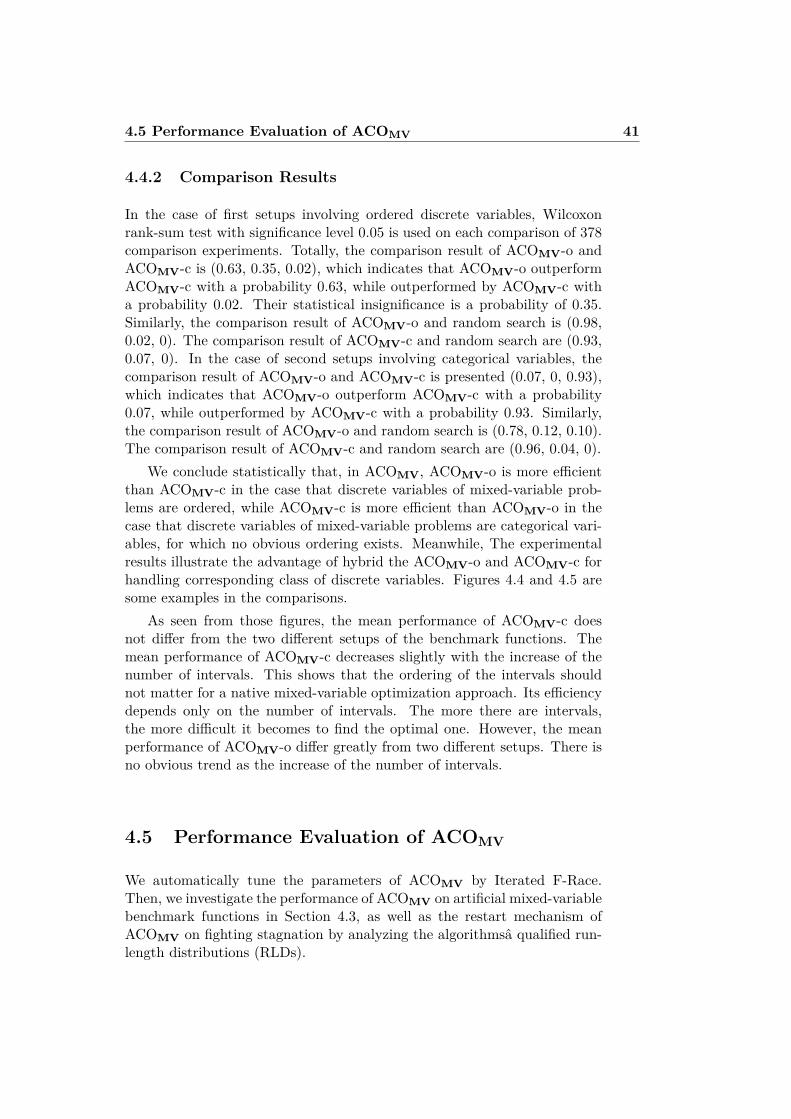
4.5 Performance Evaluation of ACOMV 41
4.4.2 Comparison Results
In the case of first setups involving ordered discrete variables, Wilcoxonrank-sum test with significance level 0.05 is used on each comparison of 378comparison experiments. Totally, the comparison result of ACOMV-o andACOMV-c is (0.63, 0.35, 0.02), which indicates that ACOMV-o outperformACOMV-c with a probability 0.63, while outperformed by ACOMV-c witha probability 0.02. Their statistical insignificance is a probability of 0.35.Similarly, the comparison result of ACOMV-o and random search is (0.98,0.02, 0). The comparison result of ACOMV-c and random search are (0.93,0.07, 0). In the case of second setups involving categorical variables, thecomparison result of ACOMV-o and ACOMV-c is presented (0.07, 0, 0.93),which indicates that ACOMV-o outperform ACOMV-c with a probability0.07, while outperformed by ACOMV-c with a probability 0.93. Similarly,the comparison result of ACOMV-o and random search is (0.78, 0.12, 0.10).The comparison result of ACOMV-c and random search are (0.96, 0.04, 0).
We conclude statistically that, in ACOMV, ACOMV-o is more efficientthan ACOMV-c in the case that discrete variables of mixed-variable prob-lems are ordered, while ACOMV-c is more efficient than ACOMV-o in thecase that discrete variables of mixed-variable problems are categorical vari-ables, for which no obvious ordering exists. Meanwhile, The experimentalresults illustrate the advantage of hybrid the ACOMV-o and ACOMV-c forhandling corresponding class of discrete variables. Figures 4.4 and 4.5 aresome examples in the comparisons.
As seen from those figures, the mean performance of ACOMV-c doesnot differ from the two different setups of the benchmark functions. Themean performance of ACOMV-c decreases slightly with the increase of thenumber of intervals. This shows that the ordering of the intervals shouldnot matter for a native mixed-variable optimization approach. Its efficiencydepends only on the number of intervals. The more there are intervals,the more difficult it becomes to find the optimal one. However, the meanperformance of ACOMV-o differ greatly from two different setups. There isno obvious trend as the increase of the number of intervals.
4.5 Performance Evaluation of ACOMV
We automatically tune the parameters of ACOMV by Iterated F-Race.Then, we investigate the performance of ACOMV on artificial mixed-variablebenchmark functions in Section 4.3, as well as the restart mechanism ofACOMV on fighting stagnation by analyzing the algorithmsâ qualified run-length distributions (RLDs).

42 Ant Colony Optimization for Mixed Variable Problems
Ackley−ordered discrete variables
Number of intervals
Me
an
f(x
)
2 101
102
103
05
10
15
20
25
30
Native mixed approach
Continuous relaxation approach
Rand search
Ackley−categorical variables
number of intervals
Me
an
f(x
)
2 101
102
103
05
10
15
20
25
30
Native mixed approach
Continuous relaxation approach
Rand search
Rastrigin−ordered discrete variables
Number of intervals
Me
an
f(x
)
2 101
102
103
01
02
03
04
05
0
Native mixed approach
Continuous relaxation approach
Rand search
Rastrigin−categorical variables
number of intervals
Me
an
f(x
)
2 101
102
103
01
02
03
04
05
0
Native mixed approach
Continuous relaxation approach
Rand search
Figure 4.4: The mean value evaluation of ACOMV-o and ACOMV-c on6 dimensional benchmark functions after 10000 evaluations, with intervalst ∈ 2, 5, 10, 20, ..., 90, 100, 200, ..., 900, 1000
.
4.5.1 Parameter Tuning of ACOMV
A crucial aspect of mixed-variable algorithms’ parameter configuration isgeneralization. Given a set of artificial mixed-variable benchmark functionsas training instances, our goal is to find high-performing algorithm param-eters that perform well on unseen problems that are not available when de-ciding on the algorithm parameters [13]. Therefore, we avoid over-tuning byapplying Iterated F-Race to artificial mixed-variable benchmark functionsrather than the engineering problems , which ACOMV are tested and com-pared in Section 4.6. For the generalization of parameters, the instances oftraining set are designed across six mixed-variable benchmark functions withmixed dimensions(2, 4, 6, 8, 10, 12, 14) [61], involving two setups of bench-mark functions,(i) with ordered discrete variables, and (ii) with categoricalvariables. We use 300 random instances and 5000 budget of experimentalevaluations in the automatic tuning procedure. The parameters obtainedare in Table 4.2. it is used for performance evaluation of ACOMV later ,and also for real world engineering optimization problems in Section 4.6.

4.5 Performance Evaluation of ACOMV 43
0 100 200 300 400 500
0.0
0.2
0.4
0.6
0.8
1.0
Rastrigin−ordered discrete variables
Number of intervals
Me
an
f(x
)
Native mixed approach
Continuous relaxation approach
0 100 200 300 400 500
0.0
0.2
0.4
0.6
0.8
1.0
Rastrigin−categorical variables
Number of intervals
Me
an
f(x
)
Native mixed approach
Continuous relaxation approach
0 100 200 300 400 500
0.0
0.5
1.0
1.5
2.0
Rosenbrock−ordered discrete variables
Number of intervals
Me
an
f(x
)
Native mixed approach
Continuous relaxation approach
0 100 200 300 400 500
0.0
0.5
1.0
1.5
2.0
Rosenbrock−categorical variables
Number of intervals
Me
an
f(x
)
Native mixed approach
Continuous relaxation approach
Figure 4.5: The mean value evaluation of ACOMV-o with ACOMV-c on2 dimensional benchmark functions after 10000 function evaluations, withintervals t ∈ 2, 5, 10, 15, ..., 490, 495, 500
Table 4.2: Summary on the tuned parameters of ACOMV.
Parameter Symbol ValueNumber of ants m 5
Speed of convergence ξ 0.05099Locality of the search q 0.6795
Archive size k 90
4.5.2 The Performance of Fighting Stagnation
Firstly, we evaluate the performance of ACOMV on the two setups of arti-ficial mixed-variable benchmark functions proposed in Section 4.3 with di-mensions (2, 6, 10). Table 4.3 shows the experimental results on the discretevariables’ intervals t = 100. ACOMV solved all 2 dimensional benchmarkfunctions with 100% success rate. ACOMV found the optimal solution ofall the 6 dimensional benchmark functions. On the 10 dimensional bench-

44 Ant Colony Optimization for Mixed Variable Problems
Ackley− categorical variables
Number of function evaluations
Pro
ba
bili
ty o
f so
lvin
g t
he
pro
ble
m
102
103
104
105
1060
.00
.20
.40
.60
.81
.0
Non−restart
Restart
Dim=2 Dim=6
Dim=10
Griewank− categorical variables
Number of function evaluations
Pro
ba
bili
ty o
f so
lvin
g t
he
pro
ble
m
102
103
104
105
1060
.00
.20
.40
.60
.81
.0
Non−restart
Restart
Dim=2 Dim=6
Dim=10
Figure 4.6: The RLDs obtained by ACOMV with restarts and withoutrestarts. The solution quality demanded is E-10
mark functions with ordered discrete variables, ACOMV found the optimalsolution of fAckleyMV
, fRosenbrockMV, fSphereMV
and fGriewankMV. On the 10
dimensional benchmark functions with categorical variables, ACOMV foundthe optimal solution of fAckleyMV
, fSphereMVand fGriewankMV
. With the in-crease of dimensionality, it is more difficult for ACOMV to find the optimalsolution. Anyway, ACOMV obtained 100% success rate to solve fAckleyMV
and fSphereMVwith both setups on the dimensions (2, 6, 10), and obtained
more than 80% success rate to solve fGriewankMVwith both setups on the
dimensions (2, 6, 10). For a detail level, Figure 4.6 shows a analysis aboutRLDs of the fAckleyMV
and fGriewankMVinvolving categorical variables. The
RLD methodology is explained in [47, 69]. Theoretical RLDs can be es-timated empirically using multiple independent runs of an algorithm. Anempirical RLD provides a graphical view of the development of the proba-bility of finding a solution of a certain quality as a function of time. In thecase of stagnation, the probability of finding a solution of a certain qualitymay be increased by a periodic restart mechanism. The restart criterionof ACOMV is the number of iterations of ants updating the archive with arelative solution improvement lower than a certain threshold ε. The num-ber of periodic iterations without significant improvement is MaxStagIter.MaxStagIter = 650, ε = 10−5 are tuned then used in restart mechanism ofACOMV. As seen from Figure 4.6, the performance of ACOMV is improvedowing to the restart mechanism on fighting against stagnation. With in-crease of dimensionality from 2 to 6 and 10, the success rate of ACOMV forsolving fAckleyMV
still maintains 100%, while the success rate of ACOMVwithout restart drops strongly. As for fGriewankMV
, the success rates ofACOMV still maintains more than 80% with the increase of dimensionalityfrom 2 to 6 and 10, while the success rate of ACOMV without restart dropsto about 20%.

4.6 Application in Engineering Optimization Problems 45
Table 4.3: Experimental results of ACOMV with dimensions D = 2, 6,10. F1 − F6 represent fEllipsoidMV
, fAckleyMV, fRastriginMV
, fRosenbrockMV,
fSphereMVand fGriewankMV
,respectively. The discrete variables’ intervalst = 100. The results are summarized over 50 independent runs, and thevalues below 1.00E-10 are approximate to 0.00E-10, which is highlighted inboldface.D Functions
Two upsets of discrete variablesOrdered discrete variables Categorical variables
Avg. Median Max. Min. Avg. Median Max. Min.
2
F1 0.00e+00 0.00e+00 0.00e+00 0.00e+00 0.00e+00 0.00e+00 0.00e+00 0.00e+00F2 0.00e+00 0.00e+00 0.00e+00 0.00e+00 0.00e+00 0.00e+00 0.00e+00 0.00e+00F3 0.00e+00 0.00e+00 0.00e+00 0.00e+00 0.00e+00 0.00e+00 0.00e+00 0.00e+00F4 0.00e+00 0.00e+00 0.00e+00 0.00e+00 0.00e+00 0.00e+00 0.00e+00 0.00e+00F5 0.00e+00 0.00e+00 0.00e+00 0.00e+00 0.00e+00 0.00e+00 0.00e+00 0.00e+00F6 0.00e+00 0.00e+00 0.00e+00 0.00e+00 0.00e+00 0.00e+00 0.00e+00 0.00e+00
6
F1 8.47e−03 0.00e+00 1.65e−01 0.00e+00 1.31e+00 4.13e−01 1.26e+01 0.00e+00F2 0.00e+00 0.00e+00 0.00e+00 0.00e+00 0.00e+00 0.00e+00 0.00e+00 0.00e+00F3 1.91+00 1.78e+00 4.38e+00 0.00e+00 2.10e+00 2.29e+00 4.38e+00 0.00e+00F4 7.82e−01 0.00e+00 1.04e+01 0.00e+00 1.00e+01 6.90e+00 5.95e+01 0.00e+00F5 0.00e+00 0.00e+00 0.00e+00 0.00e+00 0.00e+00 0.00e+00 0.00e+00 0.00e+00F6 2.43e−07 0.00e+00 1.22e−05 0.00e+00 8.41e−04 0.00e+00 1.26e−02 0.00e+00
10
F1 1.99e+00 1.40e+00 1.10e+01 1.17e−01 1.20e+01 7.32e+00 5.48e+01 5.84e−01F2 0.00e+00 0.00e+00 0.00e+00 0.00e+00 0.00e+00 0.00e+00 0.00e+00 0.00e+00F3 1.37e+01 1.48e+01 2.46e+01 2.93e+00 1.03e+01 9.65e+00 2.03e+01 3.77e+00F4 1.23e+01 1.32e+01 3.74e+01 0.00e+00 4.37e+01 1.91e+01 1.80e+02 1.03e+01F5 0.00e+00 0.00e+00 0.00e+00 0.00e+00 0.00e+00 0.00e+00 0.00e+00 0.00e+00F6 2.54e−03 0.00e+00 4.67e−02 0.00e+00 4.52e−03 0.00e+00 4.67e−02 0.00e+00
Table 4.4: Summary on the classification of engineering optimizationproblems.
Groups The type of decision variablesGroup I Continuous variables†Group II Continuous and ordered discrete variablesGroup III Continuous and categorical variablesGroup IV Continuous, ordered discrete and categorical variables† continuous variables should be a particular class of mixed variableswith empty set of discrete variables. ACOMV is also capable tosolve continuous optimization.
4.6 Application in Engineering OptimizationProblems
We have classified the engineering optimization problems in the literatureinto 4 groups according to the types of decision variables (see Table 4.4).
Group I include Welded beam design problem case A [17–19, 44, 45, 50,59, 98]; Group II include pressure vessel design problem [15, 17, 19, 22, 36,40, 44, 45, 50, 54, 58, 63, 80, 81, 91, 95, 96, 98] and the coil spring design prob-

46 Ant Colony Optimization for Mixed Variable Problems
Table 4.5: Comparison of the best solutions for welded bean design problemcase A. The infeasible solutions are highlighted in italics
Methods x1(h) x2(l) x3(t) x4(b) f(x)GA1 [17] 0.208800 3.420500 8.997500 0.210000 1.748309GA2 [19] 0.205986 3.471328 9.020224 0.206480 1.728226EP [18] 0.205700 3.470500 9.036600 0.205700 1.724852
(µ+ λ)ES [66] 0.205730 3.470489 9.036624 0.205729 1.724852CPSO [45] 0.202369 3.544214 9.048210 0.205723 1.728024HPSO [44] 0.205730 3.470489 9.033624 0.205730 1.724852
NM-PSO [98] 0.205830 3.468338 9.033624 0.205730 1.724717PSOLVER [50] 0.205830 3.468338 9.033624 0.205730 1.724717
SS [59] 0.205729 3.470489 9.033624 0.205730 1.724852ABC [5] 0.205730 3.470489 9.033624 0.205730 1.724852ACOMV 0.205729 3.470489 9.033624 0.205730 1.724852
lem [20, 22, 40, 56, 80, 96]. Group III include the thermal insulation sys-tems design [3, 6, 52]. Group IV include welded beam design problem caseB [21, 23, 95]. In this section, we compare the results obtained with thosereported in the literature in order to illustrate the performance of ACOMV.In experimental setup, the tuned parameters configuration on benchmarkfunctions are used. For outstanding the performance of ACOMV heuristicsand simplifying the algorithm, the most fundamental constraints handlingtechnique, "death penalty", is used. 100 independent runs were performedfor each engineering problem. The mathematical formulation of problemsare described in Appendix 6.1.
4.6.1 Group I : Welded Beam Design Problem Case A
Recently, many methods previously have been applied into Welded beamdesign problem case A in Appendix 6.1.1. The best solutions are comparedand list in Table 4.5. It should be noted that the results produced byNM-PSO [98] and PSOLVER [50] are infeasible solution because the thirdconstraints had been violated. Table 4.5 illustrates ACOMV obtained thebest-so-far solution. Table 4.6 illustrates the standard deviation of ACOMVresults is the smallest and ACOMV require the smallest number of functionsevaluation, 2303. The successful rate of ACOMV for best-so-far solution is100%. Accordingly, ACOMV is the most efficient and robust among theliterature in this problem. Additionally, the mean and minimum number ofevaluations of ACOMV are 2122 and 1888, respectively.

4.6 Application in Engineering Optimization Problems 47
Table 4.6: Statistical results for welded bean design problem case A. Theinfeasible solutions are highlighted in italics
Methods fBest fMean fworst Sd FEs
GA1 [17] 1.748309 1.771973 1.785835 1.12E-02 N/AGA2 [19] 1.728226 1.792654 1.993408 7.47E-02 80000EP [18] 1.724852 1.971809 3.179709 4.43E-01 N/A
(µ+ λ)ES [66] 1.724852 1.777692 NA 8.80E-02 30000CPSO [45] 1.728024 1.748831 1.782143 1.29E-02 200000HPSO [44] 1.724852 1.749040 1.814295 4.01E-02 81000
NM-PSO [98] 1.724717 1.726373 1.733393 3.50E-03 80000PSOLVER [50] 1.724717 1.724717 1.724717 1.62E-11 297
SS [59] 1.724852 1.747429 1.928811 4.67E-02 83703ABC [5] 1.724852 1.741913 NA 3.10E-02 30000ACOMV 1.724852 1.724852 1.724852 1.74E-12 2303
4.6.2 Group II: Pressure Vessel Design Problem Case A, B,C and D
There are four distinctive cases (A, B, C and D) of pressure vessel designproblem defined in the literature. These cases differ by the constraints posedon the thickness of the steel used for the heads and the main cylinder. Incase A, B, C (see Table 4.7), ACOMV obtained the best results in a 100%success rate. The number of evaluations are also the smallest. Case D ismore difficult to solve because of the larger range of side constraints fordecision variables. It should be noted that the solution of NM-PSO is notfeasible for this problem because the values of x1 and x2 given for NM-PSOare not integer multiples of 0.0625. Table 4.8 illustrates ACOMV obtainedthe best-so-far solution except the infeasible solution reported by NM-PSO .Table 4.9 illustrates ACOMV has 100% success rate to obtain the best-so-farresults with smallest standard deviation, which is competitive to PSOLVER.ACOMV require 30717 function evaluations. The mean and minimum num-ber of evaluations is 9448 and 1726. PSOLVER is more efficient in the aspectof the number of functions evaluations. However, it should be noted thatIn [50] PSOLVER is only designed for continuous optimization rather thanmixed-variable optimization, therefore, PSOLVER is difficult to solve cate-gorical variables. Moreover, PSOLVER ever reported an infeasible solutionin the previous welded beam design problem case A.
4.6.3 Group II: Coil Spring Design Problem
In coil spring design problem, most of the research reported in the literaturefocused on finding the best solution. Only the recent work by [54] and [20]
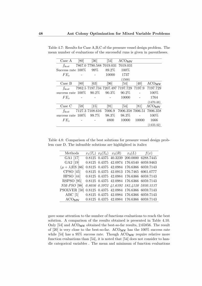
48 Ant Colony Optimization for Mixed Variable Problems
Table 4.7: Results for Case A,B,C of the pressure vessel design problem. Themean number of evaluations of the successful runs is given in parentheses.
Case A [80] [36] [54] ACOMVfbest 7867.0 7790.588 7019.031 7019.031
Success rate 100% 99% 89.2% 100%FEs - - 10000 1737
(1500)Case B [80] [63] [96] [54] [40] ACOMVfbest 7982.5 7197.734 7207.497 7197.729 7197.9 7197.729
success rate 100% 90.2% 90.3% 90.2% - 100%FEs - - - 10000 - 1764
(1470.48)Case C [58] [15] [91] [54] [81] ACOMVfbest 7127.3 7108.616 7006.9 7006.358 7006.51 7006.358
success rate 100% 99.7% 98.3% 98.3% - 100%FEs - - 4800 10000 10000 1666
(1433.42)
Table 4.8: Comparison of the best solutions for pressure vessel design prob-lem case D. The infeasible solutions are highlighted in italics
Methods x1(Ts) x2(Th) x3(R) x4(L) f(x)GA1 [17] 0.8125 0.4375 40.3239 200.0000 6288.7445GA2 [19] 0.8125 0.4375 42.0974 176.6540 6059.9463
(µ+ λ)ES [66] 0.8125 0.4375 42.0984 176.6366 6059.7143CPSO [45] 0.8125 0.4375 42.0913 176.7465 6061.0777HPSO [44] 0.8125 0.4375 42.0984 176.6366 6059.7143RSPSO [95] 0.8125 0.4375 42.0984 176.6366 6059.7143NM-PSO [98] 0.8036 0.3972 41.6392 182.4120 5930.3137PSOLVER [50] 0.8125 0.4375 42.0984 176.6366 6059.7143
ABC [5] 0.8125 0.4375 42.0984 176.6366 6059.7143ACOMV 0.8125 0.4375 42.0984 176.6366 6059.7143
gave some attention to the number of functions evaluations to reach the bestsolution. A comparison of the results obtained is presented in Table 4.10.Only [54] and ACOMV obtained the best-so-far results, 2.65856. The resultof [20] is very close to the best-so-far. ACOMV has the 100% success ratewhile [54] has a 95% success rate. Though ACOMV require relative morefunction evaluations than [54], it is noted that [54] does not consider to han-dle categorical variables . The mean and minimum of function evaluations

4.6 Application in Engineering Optimization Problems 49
Table 4.9: Statistical results for pressure vessel design problem case D . Themean number of evaluations of the successful runs is given in parentheses.The infeasible solutions are highlighted in italics
Methods fBest fMean fworst Sd FEs
GA1 [17] 6288.7445 6293.8432 6308.1497 7.413E+00 N/AGA2 [19] 6059.9463 6177.2533 6469.3220 1.309E+02 80000
(µ+ λ)ES [66] 6059.7143 6379.938037 NA 2.10E+02 30000CPSO [45] 6061.0777 6147.1332 6363.8041 8.645E+01 200000HPSO [44] 6059.7143 6099.9323 6288.6770 8.620E+01 81000RSPSO [95] 6059.7143 6066.2032 6100.3196 1.33E+01 30000NM-PSO [98] 5930.3137 5946.7901 5960.0557 9.161E+00 80000PSOLVER [50] 6059.7143 6059.7143 6059.7143 4.625E-12 310
ABC [5] 6059.7143 6245.3081 NA 2.05E+02 30000ACOMV 6059.7143 6059.7143 6059.7143 3.45E-12 30717
(9448.08)
Table 4.10: Results for the coil spring design problem. The mean numberof evaluations of the successful runs is given in parentheses.
[80] [16] [96] [54] [40] [20] ACOMVN 10 9 9 9 9 9 9
D [inch] 1.180701 1.2287 1.227411 1.223041 1.223 1.223044 1.223041d [inch] 0.283 0.283 0.283 0.283 0.283 0.283 0.283fbest 2.7995 2.6709 2.6681 2.65856 2.659 2.658565 2.65856
success rate 100% 95.4% 95.3% 95.0% - <100% 100%FEs - - - 8000 - 3711560
(2270994)19588
(4808.19)
of ACOMV are 9948 and 1726. [20] does not report a success rate, but thecorresponding objective value vary in the range of (2.658565, 2.658790), thenumbers of function evaluation vary in the range of [539960, 3711560].
4.6.4 Group III: Thermal Insulation Systems DesignProblem
The thermal insulation systems design problem is one of the few benchmarkengineering problems used in the literature that deals with categorical vari-ables. In previous studies, the categorical variables describing the type ofinsulators used indifferent layers were not considered as optimization vari-able, but rather as parameters. Only the more recent work of Kokkolaras

50 Ant Colony Optimization for Mixed Variable Problems
et al [52] and Abramson et al [3], which are able to handle such categori-cal variables properly. we show that ACOMV can performs comparably toMVP [52] and FMGPS [3]. Table 4.11 present the new best-so-far solutionof ACOMV after 10000 function evalutations.
4.6.5 Group IV: Welded Beam Design Problem Case B
Welded beam design problem case B is taken from Deb and Goyal [21] andDimopoulos [23]. It is a variation of case A and is extended to include or-dered discrete and categorical variables together. Table 4.12 shows ACOMVobtained a new best-so-far solution with a 100% success rate. The maxi-mum, mean and minimum number of evaluations of is 4883, 1436 and 692,respectively. Table 4.14 verifies the best results obtained by ACOMV not toviolate the constraints.
4.6.6 Related Work on Engineering Optimization Problems
For a detail level analysis on engineering optimization problems, we inves-tigate ACOMV RLDs on fighting against stagnation by restart mechanism.An experiment is also conducted to compare the performance of the genericrestart mechanism of ACOMV with a problem tailored restart mechanism,called cut-off restart. The later is based on an approximation of exponen-tial distribution. It is possible to estimate, from an empirically estimatedRLD, the number of function evaluations needed to find the required solu-tion with a probability greater than or equal to z if an optimal restart policyis supposed to be used. This estimation is sometimes called computationaleffort [69,73] and it is defined as
effort = min(l)l · ln(1− z)ln(1−RLq(l))
(4.5)
The solution l of the computation effort is the cut-off evaluations to peri-odically restart in a simulation of estimate model. RLq(l) is the algorithm’sRLD, defined as RLq(l) = P (Lq ≤ l), where Lq is the random variablerepresenting the number of function evaluations needed to find a solutionof quality q, and P (Lq ≤ l) is the probability that Lq takes a value lessthan or equal to l function evaluations. The cut-off restart improves theperformance of algorithms as seen from Figure 4.7. However we also seethat the tuned restart mechanism of ACOMV needs less functions evalua-tions to have 100% success rate than the cut-off restart, even if latter oneis problem-tailored. Taking the pressure vessel design problem case D ofFigure 4.7 for example, the cut-off restart starts at the point (2243 functionevaluations with a 23% success rate), and obtain a 99% success rate with44400 function evaluations, while the tuned restart mechanism of ACOMV

4.7 Conclusions 51
0 10000 30000 50000
0.0
0.2
0.4
0.6
0.8
1.0
pvdD
Function evaluations
Pro
ba
bili
ty o
f so
lvin
g t
he
pro
ble
m
Cut−off:( 2243 , 0.23 )
(30717,1.0)(44400,0.99)
ACOmv
Non−restart
Estimated mode
Cut−off restart
csd
Function evaluations
Pro
ba
bili
ty o
f so
lvin
g t
he
pro
ble
m
103
104
1050
.00
.20
.40
.60
.81
.0
Cut−off:( 2373 , 0.62 )
(19588,1.0)
(25192,1.0)
ACOmv
Non−restart
Estimated mode
Cut−off restart
wbdm
Function evaluations
Pro
ba
bili
ty o
f so
lvin
g t
he
pro
ble
m
600 103
1040
.00
.20
.40
.60
.81
.0
Cut−off:( 1188 , 0.88 )
(4883,1.0)
(5404,1.0)
ACOmv
Non−restart
Estimated mode
Cut−off restart
Figure 4.7: the RLDs analysis of ACOMV on engineering optimization prob-lems. pvdD is the pressure vessel design problem case D. Csd is the coilspring design problem. WbdB is the welded beam design problem case B
needs 30717 function evaluations to obtain a 100% success rate. Addition-ally, it is mentioned that in the welded beam design case A and the pressurevessel design problem case A, B and C, we found that ACOMV withoutrestarts mechanism has not met any stagnation cases and has 100% successrate to give the best-so-far solution. So, we analyze on the problems, inwhich the restart mechanism takes effect.
4.7 Conclusions
In this chapter, we have shown how ACOR is extended to ACOMV for tack-ling mixed-variable optimization problems. Based on the solution archiveframework of ACOMV, ACOMV integrates a component of a continuousoptimization solver (ACOR), a continuous relaxation approach (ACOMV-o) and a native mixed-variable optimization approach (ACOMV-c) to solvecontinuous and mixed-variable optimization problems. In addition, we pro-posed artificial mixed-variable benchmark functions as well as constructivemethods. They provide a sufficiently controlled environment for the in-

52 Ant Colony Optimization for Mixed Variable Problems
vestigation of the performance of mixed-variable optimization algorithms,and they provide a training environment for parameter tuning. Based onthe benchmark functions, a rigorous comparison between ACOMV-o andACOMV-c was conducted, so that we can conclude from these results of thiscomparision that ACOMV-o is better than ACOMV-c in the case that thediscrete variables of mixed-variable problems are ordered, while ACOMV-cis better than ACOMV-o in the case that discrete variables of mixed-variableproblems are categorical variables. The experiments illustrate the advantageof combining of ACOMV-o and ACOMV-c, and also suggest that discardingof scratching one of them to handle mixed-variable optimization problems isnot a good idea. The experimental results for real-world engineering prob-lems illustrate that ACOMV not only can tackle various classes of decisionvariables robustly, but also it is efficient in finding high-quality solutions. Inthe welded beam design case A and the pressure vessel design problem caseA, B, C, ACOMV is the only available algorithm that obtains the best-so-farsolution with a 100% success rate as well as the required smallest number offunction evaluations. In the pressure vessel design problem case D, ACOMVobtains the best-so-far solution with a 100% success rate. In the coil springdesign problem, ACOMV is the only one that obtains the best-so-far solu-tion with a 100% success rate. In the thermal insulation systems designproblem, ACOMV obtains the new best-so-far solution. In the welded beamdesign problem case B, ACOMV obtained the new best-so-far solution witha 100% success rate and the smallest number of function evaluations.

4.7 Conclusions 53
Table 4.11: Comparison of the best solutions for the thermal insulationsystems
Solution information MVP [52] FMGPS [3] ACOMVContinuous variable
xi(cm)1 0.3125 4.5313 4.95062 5.4688 6.7188 7.97293 3.9062 4.8437 12.84484 6.5625 4.2188 17.079785 5.7812 7.3438 9.44206 5.1562 9.8438 10.10777 13.2812 24.948 0.028118 21.4062 12.135 7.30809 8.5938 7.5 11.959210 9.2188 6.4063 12.187211 20.3125 11.5105 6.1197
Ti(K)1 4.2188 6.125 6.10032 7.3438 10.55 11.08413 10 14.35 21.25094 15 17.994 38.26085 20 24.969 51.85086 25 36.006 70.10007 40 71.094 71.00018 71.0938 116.88 99.44759 101.25 156.88 153.170110 146.25 198.44 236.835811 300 300 300
Categorical variableIi1 N N N2 N N N3 N N N4 N N N5 N N T6 N N E7 N T T8 E E E9 E E E10 E T T11 T T T
Power(PLA ( Wcm)) 25.294 25.58 24.299

54 Ant Colony Optimization for Mixed Variable Problems
Table 4.12: Comparison of the best solutions for welded beam design designproblem case B
Methods x1(h) x2(l) x3(t) x4(b) x5(M) x6(Joint) f(x)GeneAS [21] 0.1875 1.6849 8.2500 0.2500 Steel 4-sided 1.9422PSOA [23] 0.2500 2.2219 8.2500 0.2500 Steel 2-sided 1.7631RSPSO [95] 0.1875 1.6842 8.25 0.25 Steel 4-sided 1.9421ACOMV 0.225 1.272373 8.25 0.225 Steel 4-sided 1.502942
Table 4.13: Statistical results for welded beam design design problem caseB
Methods fMean Sd FEs
GeneAS [21] N/A N/A N/ARSPSO [95] N/A N/A N/APSOA [23] 1.7631 0 6570ACOMV 1.502942 0 1436
Table 4.14: Constrains analysis for welded beam design design problem caseB
Constraints GeneAS [21] PSOA [23] RSPSO [95] ACOMVg1 -0.1621 0 N/A 0g2 -380.1660 N/A -380.1653 -148.8186g3 -0.0625 0 N/A 0g4 -3.4399 -3.3838 N/A -3.562618g5 -0.0625 -0.1250 N/A -0.1g6 -0.2346 -0.2344 N/A -0.2349907g7 -402.0473 -412.5254 N/A -1630.64

Chapter 5
Conclusions and FutureWork
5.1 Conclusions
In this thesis, we have proposed two improved ant colony optimization algo-rithms for continuous and mixed discrete-continuous optimization problems.These are IACOR-LS and ACOMV, respectively.
In Chapter 2, based on the new C++ implementation of ACOR andSep-ACOR, we further investigated their performance and addressed theirpossible drawbacks.
Then, we proposed IACOR-LS, an ACOR algorithm with growing solu-tion archive hybridized with a local search procedure in Chapter 3. Threedifferent local search procedures, Powell’s conjugate directions set, Powell’sBOBYQA, and Mtsls1, were tested with IACOR-LS in order to enhanceits search intensification. The very good performance of IACOR-Mtsls1 isa clear indication of the high potential hybrid ACO algorithms have forthe continuous domain. In fact, IACOR-Mtsls1 is clearly competitive withstate-of-the-art continuous optimizers.
In Chapter 4 , we have shown how ACOR is extended to ACOMVfor tackling mixed-variable optimization problems. Based on the solu-tion archive framework of ACOMV, ACOMV integrates a component ofa continuous optimization solver (ACOR), a continuous relaxation approach(ACOMV-o) and a native mixed-variable optimization approach (ACOMV-c) to solve continuous and mixed-variable optimization problems. In addi-tion, we proposed artificial mixed-variable benchmark functions as well asconstructive methods. They provide a sufficiently controlled environmentfor the investigation of the performance of mixed-variable optimization al-gorithms, and they provide a training environment for parameter tuning.Based on the benchmark functions, a rigorous comparison between ACOMV-o and ACOMV-c was conducted, so that we can conclude from these results

56 Conclusions and Future Work
of this comparision that ACOMV-o is better than ACOMV-c in the casethat the discrete variables of mixed-variable problems are ordered, whileACOMV-c is better than ACOMV-o in the case that discrete variables ofmixed-variable problems are categorical variables. The experiments illus-trate the advantage of combining of ACOMV-o and ACOMV-c, and alsosuggest that discarding of scratching one of them to handle mixed-variableoptimization problems is not a good idea. The experimental results forreal-world engineering problems illustrate that ACOMV not only can tacklevarious classes of decision variables robustly, but also it is efficient in findinghigh-quality solutions. In the welded beam design case A and the pressurevessel design problem case A, B, C, ACOMV is the only available algorithmthat obtains the best-so-far solution with a 100% success rate as well as therequired smallest number of function evaluations. In the pressure vessel de-sign problem case D, ACOMV obtains the best-so-far solution with a 100%success rate. In the coil spring design problem, ACOMV is the only one thatobtains the best-so-far solution with a 100% success rate. In the thermalinsulation systems design problem, ACOMV obtains the new best-so-far so-lution. In the welded beam design problem case B, ACOMV obtained thenew best-so-far solution with a 100% success rate and the smallest numberof function evaluations.
5.2 Future Work
In practice, high dimensional and highly variable-correlated continuous opti-mization problems also need to be optimized. Therefore, a new effective andefficient variable correlation method for ACOR is one of our ongoing works.Moreover, for implementing a high-performing continuous algorithm, we areinvestigating and fairly benchmarking state-of-the-art continuous optimiza-tion algorithms. Since, different continuous optimization algorithms maybe preferably depending on the characteristics of problems, one promisingdirection we intend to research on is to automatically select and configurecontinuous optimizers from components, thereby facing challenging contin-uous instances with different characteristics.
In the aspect of ACO for mixed discrete-continuous optimization, thesolution archive of ACOMV consists in a flexible framework that allows tobring in a resizing population strategy and a hybrid with a subsidiary localsearch procedure. The incremental population social learning mechanismwith local search [60, 68, 70, 71] in Chaper 3 is an interesting modificationfor ACOMV. Powell’s conjugate directions set [76], Powell’s BOBYQA [77],and Lin-Yu Tseng’s Mtsls1 methods [93] and Hansen’s CMA-ES [41] arebeing considered to be hybridized with ACOMV for continuous variablesand ordered discrete variables. Some typical local search in discrete opti-mization are considered for handling categorical variables. We also intend

5.2 Future Work 57
to develop an effective constraint-handling technique based on the ACOMVframework to tackle highly challenging constrained mixed-variable optimiza-tion applications. Finally, a tuning-in-the-loop approach [71] is to be used toredesign ACOMV. A promising application of ACOMV is that the heuristicsof ACOMV meet the variables arising in the algorithm configuration prob-lem [13], in which typically not only the setting of numerical parametersbut also that of categorical parameters needs to be determined. Recently,in [97], several continuous algorithms have been used with F-race [12] toautomatically tune parameters from real variable and large ordinal integervariables. ACOMV with F-race to tackle mixed-variable parameters includ-ing categorical variable is also our following work.


Chapter 6
Appendix
6.1 Mathematical formulation of engineeringproblems
6.1.1 Welded Beam Design Problem Case A
The mathematical formulation of the welded beam design problem is givenin Table 6.1. The schema is shown in Figure 6.1
6.1.2 Welded Beam Design Problem Case B
The welded beam design problem case B is a variation of case A. It isextended to include two types of welded joint configuration and four possiblebeam materials. The changed places with respect to the formulation in Table6.1 are shown in Equation 6.1.
Figure 6.1: Schematic of welded beam design problem case A.

60 Appendix
Table 6.1: The mathematical formulation of the welded beam design prob-lem case A.
min f(~x) = 1.10471x21x2 + 0.04811x3x4 (14 + x2)
g1 τ(~x)− τmax ≤ 0g2 σ(~x)− σmax ≤ 0g3 x1 − x4 ≤ 0g4 0.10471x2
1 + 0.04811x3x4 (14 + x2)− 5 ≤ 0g5 0.125− x1 ≤ 0g6 δ(~x)− δmax ≤ 0g7 P − Pc(~x) ≤ 0g8 0.1 ≤ x1, x4 ≤ 2.0g9 0.1 ≤ x2, x3 ≤ 10.0
where τ(~x) =√
(τ ′)2 + 2τ ′τ ′′ x22R + (τ ′′)2
τ ′ = P√2x1x2
, τ ′′ = MRJ ,M = P (L+ X2
2 )
R =√
x22
4 + (x1+x32 )2
J = 2√
2x1x2[x2
212 +
(x1+x32)2]
σ(~x) = 6PLx4x2
3, δ(x) = 4PL3
Ex33x4
Pc(~x) = 4.013E√
x23x
64
36L2
(1− x3
2L
√E4G
)P = 6000lb, L = 14in., E = 30× 106psi,G = 12× 106psi
τmax = 1360psi, σmax = 30000psi, δ = 0.25in.
Table 6.2: Material properties for the welded beam design problem case B
Methods x5 S(103psi) E(106psi) G(106psi) c1 c2
Steel 30 30 12 0.1047 0.0481Cast iron 8 14 6 0.0489 0.0224Aluminum 5 10 4 0.5235 0.2405
Brass 8 16 6 0.5584 0.2566
min f(~x) = (1 + c1)x21x2 + c2 x3x4 (14 + x2)
S − τmax ≤ 0J = 2
√2x1x2
[x2
212 +
(x1+x32)2]
, if x6 : two sideJ = 2
√2x1x2
[x2
212 +
(x1+x32)2]
, if x6 : four sideτmax = 0.577 · S
(6.1)

6.1 Mathematical formulation of engineering problems 61
Figure 6.2: Schema of the pressure vessel to be designed.
Table 6.3: The mathematical formulation of the cases (A, B, C and D) ofthe pressure vessel design problem.
No Case A Case B Case C Case Dmin f = 0.6224TsRL+ 1.7781ThR2 + 3.1611T 2
s L+ 19.84T 2sR
g1 −Ts + 0.0193R ≤ 0g2 −Th + 0.00954R ≤ 0g3 −π R2L− 4
3π R3 + 750 · 1728 ≤ 0
g4 L− 240 ≤ 0g5 1.1 ≤ Ts ≤ 12.5 1.125 ≤ Ts ≤ 12.5 1 ≤ Ts ≤ 12.5 0 ≤ Ts ≤ 100g6 0.6 ≤ Th ≤ 12.5 0.625 ≤ Th ≤ 12.5 0 ≤ Th ≤ 100g7 0.0 ≤ R ≤ 240 10 ≤ R ≤ 200g8 0.0 ≤ L ≤ 240 10 ≤ L ≤ 200
6.1.3 Pressure Vessel Design Problems
The pressure vessel design problems requires designing a pressure vesselconsisting of a cylindrical body and two hemispherical heads such that thecost of its manufacturing is minimized subject to certain constraints. Theschematic picture of the vessel is presented in Figure 6.2. There are fourvariables where values must be chosen: the thickness of the main cylinderTs, the thickness of the heads Th, the inner radius of the main cylinderR, and the length of the main cylinder L. While variables R and L arecontinuous, the thickness for variables Ts and Th may be chosen only from aset of allowed values, these being the integer multiples of 0.0625 inch. Themathematical formulation for the cases (A, B, C and D) is given in Table 6.3.
6.1.4 Coil Spring Design Problem
The problem consists in designing a helical compression spring that willhold an axial and constant load. The objective is to minimize the volumeof the spring wire used to manufacture the spring. A schematic of the coilspring to be designed is shown in Figure 6.3. The decision variables are thenumber of spring coils N , the outside diameter of the spring D, and thespring wire diameter d. The number of coils N is an integer variable, theoutside diameter of the spring D is a continuous variable, and finally, thespring wire diameter is a discrete variable, whose possible values are given

62 Appendix
Figure 6.3: Schematic of the coil spring to be designed.
Table 6.4: Standard wire diameters available for the spring coil.
Allowed wire diameters [inch]0.0090 0.0095 0.0104 0.0118 0.0128 0.01320.0140 0.0150 0.0162 0.0173 0.0180 0.02000.0230 0.0250 0.0280 0.0320 0.0350 0.04100.0470 0.0540 0.0630 0.0720 0.0800 0.09200.1050 0.1200 0.1350 0.1480 0.1620 0.17700.1920 0.2070 0.2250 0.2440 0.2630 0.28300.3070 0.3310 0.3620 0.3940 0.4375 0.5000
Figure 6.4: Schematic of the thermal insulation system.
in Table 6.4. The mathematical formulation is in Table 6.5. The penaltyfunction was defined in Equation 6.2, which is the similar to [56] for a morerigorous heuristics comparison between ACOMV and Differential Evolution.
f = fc∏8i=1 c
3i ,
ci =
1 + sigi if gi > 0,1 otherwise,
s1 = 10−5, s2 = s4 = s6 = 1, s3 = s5 = s7 = s8 = 102.
(6.2)

6.1 Mathematical formulation of engineering problems 63
Table 6.5: The mathematical formulation for the coil spring design problem.
min fc(N,D, d) = π2 Dd2(N+2)4
No Constraintg1
8CfFmaxDπ d − S ≤ 0
g2 lf − lmax ≤ 0g3 dmin − d ≤ 0g4 D −Dmax ≤ 0g5 3.0− D
d ≤ 0g6 σp − σpm ≤ 0g7 σp + Fmax−Fp
K + 1.05(N + 2)d− lf ≤ 0g8 σw − Fmax−Fp
K ≤ 0where Cf = 4D
d−1
4Dd−4 + 0.615 d
D
K = Gd4
8ND3
σp = FpK
lf = FmaxK + 1.05(N + 2)d
6.1.5 Thermal Insulation Systems Design Problem
The schema is shown in Figure 6.4. The basic mathematical formulationof the classic model of thermal insulation systems is defined in Table 6.6.The effective thermal conductivity k of all these insulators varies with thetemperature and does so differently for different materials. Considering thatthe number of intercepts n is defined in advance, and based on the presentedmodel, we may define the following problem variables:
• Ii ∈M, i = 1, ..., n+1 — the material used for the insulation betweenthe (i− 1)-st and the i-th intercepts (from a set M of materials).
• ∆xi ∈ R+, i = 1, ..., n + 1 — the thickness of the insulation betweenthe (i− 1)-st and the i-th intercepts.
• ∆Ti ∈ R+, i = 1, ..., n+ 1 — the temperature difference of the insula-tion between the (i− 1)-st and the i-th intercepts.
This way, there are n + 1 categorical variables chosen form a set M ofavailable materials. The remaining 2n+ 2 variables are continuous.

64 Appendix
Table 6.6: The mathematical formulation for the coil spring design problem.
f(x,T) = ∑ni=1 Pi = ACi
(ThotTi− 1
)∫ Ti+1Ti
kdT
∆xi −∫ TiTi−1
kdT
∆xi−1
No Constraintg1 ∆xi ≥ 0, i = 1, ..., n+ 1g2 Tcold ≤ T1 ≤ T2 ≤ ... ≤ Tn−1 ≤ Tn ≤ Thotg3
∑n+1i=1 ∆xi = L
where C = 2.5 if T ≥ 71KC = 4 if 71K > T > 4.2K
C = 5 if T ≤ 4.2K

Bibliography
[1] K. Abhishek, S. Leyffer, and J.T. Linderoth. Modeling without categori-cal variables: a mixed-integer nonlinear program for the optimization ofthermal insulation systems. Optimization and Engineering, 11(2):185–212, 2010.
[2] M.A. Abramson. Pattern search algorithms for mixed variable generalconstrained optimization problems. PhD thesis, Rice University, USA,2002.
[3] M.A. Abramson. Mixed variable optimization of a load-bearing thermalinsulation system using a filter pattern search algorithm. Optimizationand Engineering, 5(2):157–177, 2004.
[4] M.A. Abramson, C. Audet, J.W. Chrissis, and J.G. Walston. Meshadaptive direct search algorithms for mixed variable optimization. Op-timization Letters, 3(1):35–47, 2009.
[5] B. Akay and D. Karaboga. Artificial bee colony algorithm for large-scaleproblems and engineering design optimization. Journal of IntelligentManufacturing, pages 1–14, 2010.
[6] C. Audet and J.E. Dennis Jr. Pattern search algorithms for mixedvariable programming. SIAM Journal on Optimization, 11(3):573–594,2001.
[7] A. Auger and N. Hansen. A restart CMA evolution strategy with in-creasing population size. In Proceedings of IEEE Congress on Evo-lutionary Computation, CEC 2005, pages 1769–1776, Piscataway, NJ,2005. IEEE Press.
[8] A. Auger, N. Hansen, J. Perez Zerpa, R. Ros, and M. Schoenauer.Experimental comparisons of derivative free optimization algorithms.In Jan Vahrenhold, editor, Experimental Algorithms, volume 5526 ofLNCS, pages 3–15, Berlin, Germany, 2009. Springer.
[9] P. Balaprakash, M. Birattari, and T. Stützle. Improvement strategiesfor the F-Race algorithm: Sampling design and iterative refinement. In

66 BIBLIOGRAPHY
Proceedings of the 4th international conference on Hybrid metaheuris-tics, volume 4771 of LNCS, pages 108–122, Berlin, Germany, 2007.Springer.
[10] G. Bilchev and I.C. Parmee. The ant colony metaphor for searchingcontinuous design spaces. In Terence C. Fogarty, editor, Proceedingsof the AISB Workshop on Evolutionary Computation, volume 993 ofLNCS, pages 25–39. Springer-Verlag, Berlin, Germany, 1995.
[11] M. Birattari. The Problem of Tuning Metaheuristics as Seen From aMachine Learning Perspective. PhD thesis, volume 292 of Dissertatio-nen zur Künstlichen Intelligenz. Akademische Verlagsgesellschaft AkaGmbH, Berlin, Germany, 2005.
[12] M. Birattari, T. Stützle, L. Paquete, and K. Varrentrapp. A racing al-gorithm for configuring metaheuristics. In W. B. Langdon et al., editor,Proceedings of the Genetic and Evolutionary Computation Conference,pages 11–18. Morgan Kaufman, San Francisco, CA, 2002.
[13] M. Birattari, Z. Yuan, P. Balaprakash, and T. Stützle. F-Race anditerated F-Race: An overview. Experimental Methods for the Analysisof Optimization Algorithms, pages 311–336, 2010.
[14] Christian Blum, M. Yábar Vallès, and María J. Blesa. An ant colonyoptimization algorithm for DNA sequencing by hybridization. Comput-ers & Operations Research, 35(11):3620–3635, 2008.
[15] Y.J. Cao and Q.H. Wu. Mechanical design optimization by mixed-variable evolutionary programming. In Proceedings of IEEE Conferenceon Evolutionary Computation, pages 443–446, Piscataway, NJ, 1997.IEEE Press.
[16] J.L. Chen and Y.C. Tsao. Optimal design of machine elements us-ing genetic algorithms. CHUNG-KUO CHI HSUEH KUNG CH’ENGHSUEH PAO., 14(2):193–199, 1993.
[17] C. Coello and A. Carlos. Use of a self-adaptive penalty approach forengineering optimization problems. Computers in Industry, 41(2):113–127, 2000.
[18] C.A.C. Coello and R.L. Becerra. Efficient evolutionary optimizationthrough the use of a cultural algorithm. Engineering Optimization,36(2):219–236, 2004.
[19] C.A. Coello Coello and E. Mezura Montes. Constraint-handling ingenetic algorithms through the use of dominance-based tournament se-lection. Advanced Engineering Informatics, 16(3):193–203, 2002.

BIBLIOGRAPHY 67
[20] D. Datta and J. Figueira. A Real-Integer-Discrete-Coded DifferentialEvolution Algorithm: A Preliminary Study. Evolutionary Computationin Combinatorial Optimization, pages 35–46, 2010.
[21] K. Deb and M. Goyal. A combined genetic adaptive search (GeneAS)for engineering design. Computer Science and Informatics, 26:30–45,1996.
[22] K. Deb and M. Goyal. A flexible optimiztion procedure for mechan-ical component design based on genetic adaptive search. Journal ofMechanical Design, 120(2):162–164, 1998.
[23] G.G. Dimopoulos. Mixed-variable engineering optimization based onevolutionary and social metaphors. Computer methods in applied me-chanics and engineering, 196(4-6):803–817, 2007.
[24] M. Dorigo. Optimization, Learning and Natural Algorithms (in Italian).PhD thesis, Dipartimento di Elettronica, Politecnico di Milano, Italy,1992.
[25] M. Dorigo, V. Maniezzo, and A. Colorni. Ant System: Optimization bya colony of cooperating agents. IEEE Transactions on Systems, Man,and Cybernetics – Part B, 26(1):29–41, 1996.
[26] M. Dorigo and T. Stützle. Ant Colony Optimization. MIT Press, Cam-bridge, MA, 2004.
[27] Marco Dorigo and Christian Blum. Ant colony optimization theory: Asurvey. Theoretical Computer Science, 344(2-3):243–278, 2005.
[28] Marco Dorigo, G. Di Caro, and L. M. Gambardella. Ant algorithms fordiscrete optimization. Artificial Life, 5(2):137–172, 1999.
[29] Marco Dorigo and L. M. Gambardella. Ant Colony System: A coop-erative learning approach to the traveling salesman problem. IEEETransactions on Evolutionary Computation, 1(1):53–66, 1997.
[30] Marco Dorigo, Vittorio Maniezzo, and Alberto Colorni. Ant System:Optimization by a colony of cooperating agents. IEEE Transactions onSystems, Man, and Cybernetics – Part B, 26(1):29–41, 1996.
[31] Marco Dorigo and Thomas Stützle. Ant colony optimization: Overviewand recent advances. In M. Gendreau and J.-Y. Potvin, editors, Hand-book of Metaheuristics, volume 146 of International Series in Opera-tions Research & Management Science, pages 227–263. Kluwer Aca-demic Publishers, Boston, MA, 2010.

68 BIBLIOGRAPHY
[32] J. Dréo and P. Siarry. A new ant colony algorithm using the heterarchi-cal concept aimed at optimization of multiminima continuous functions.In M. Dorigo, G. Di Caro, and M. Sampels, editors, Proceedings of theThird International Workshop on Ant Algorithms, ANTS 2002, volume2463 of LNCS, pages 216–221, Berlin, Germany, 2002. Springer-Verlag.
[33] J. Dréo and P. Siarry. Continuous interacting ant colony algorithmbased on dense heterarchy. Future Generation Computer Systems,20(5):841–856, 2004.
[34] A.E. Eiben and T. Bäck. Empirical investigation of multiparent recom-bination operators in evolution strategies. Evolutionary Computation,5(3):347–365, 1997.
[35] L.J. Eshelman and J.D. Schaffer. Real-coded genetic algorithms andinterval-schemata. Foundations of Genetic Algorithms, 2(1993):187–202, 1993.
[36] J.-F. Fu, R.G. Fenton, and W.L. Cleghorn. A mixed integer-discrete-continuous programming method and its application to engineering de-sign optimization. Engineering Optimization, 17(4):263–280, 1991.
[37] L. M. Gambardella, Éric D. Taillard, and G. Agazzi. MACS-VRPTW:A multiple ant colony system for vehicle routing problems with timewindows. In David Corne, Marco Dorigo, and F. Glover, editors, NewIdeas in Optimization, pages 63–76. McGraw Hill, London, UK, 1999.
[38] D.E. Goldberg. Genetic algorithms in search, optimization, and ma-chine learning. Addison-wesley, 1989.
[39] G.H. Golub and C.F. Van Loan. Matrix computations. Johns HopkinsUniversity Press, Baltimore, MD, 1989.
[40] C. Guo, J. Hu, B. Ye, and Y. Cao. Swarm intelligence for mixed-variable design optimization. Journal of Zhejiang University Science,5(7):851–860, 2004.
[41] N. Hansen and A. Ostermeier. Completely derandomized self-adaptation in evolution strategies. Evolutionary Computation,9(2):159–195, 2001.
[42] N. Hansen, A. Ostermeier, and A. Gawelczyk. On the adaptation ofarbitrary normal mutation distributions in evolution strategies: Thegenerating set adaptation. In Proc. of 6th ICGA, pages 57–64, SanFrancisco, CA, 1995. Morgan Kaufmann.
[43] N. Hansen, R. Ros, N. Mauny, M. Schoenauer, and A. Auger. PSOfacing non-separable and ill-conditioned problems. Technical report,INRIA, 2008.

BIBLIOGRAPHY 69
[44] Q. He and L. Wang. A hybrid particle swarm optimization with afeasibility-based rule for constrained optimization. Applied Mathematicsand Computation, 186(2):1407–1422, 2007.
[45] Q. He and L. Wang. An effective co-evolutionary particle swarm op-timization for constrained engineering design problems. EngineeringApplications of Artificial Intelligence, 20(1):89–99, 2007.
[46] F. Herrera, M. Lozano, and D. Molina. Test suite for the special issueof soft computing on scalability of evolutionary algorithms and othermetaheuristics for large scale continuous optimization problems, 2010.URL: http://sci2s.ugr.es/eamhco/updated-functions1-19.pdf.
[47] H.H. Hoos and T. Stützle. Stochastic local search: Foundations andapplications. Morgan Kaufmann, San Francisco, CA, 2005.
[48] R. Ihaka and R. Gentleman. R: A language for data analysis andgraphics. Journal of computational and graphical statistics, 5(3):299–314, 1996.
[49] S.G. Johnson. The NLopt nonlinear-optimization package, 2009.
[50] A.H. Kayhan, H. Ceylan, M.T. Ayvaz, and G. Gurarslan. PSOLVER:A new hybrid particle swarm optimization algorithm for solving con-tinuous optimization problems. Expert Systems with Applications,37(10):6798–6808, 2010.
[51] J. Kennedy, R.C. Eberhart, and Y. Shi. Swarm intelligence. MorganKaufmann, San Francisco, CA, 2001.
[52] M. Kokkolaras, C. Audet, and J.E. Dennis Jr. Mixed variable opti-mization of the number and composition of heat intercepts in a thermalinsulation system. Optimization and Engineering, 2(1):5–29, 2001.
[53] O. Korb, T. Stützle, and T.E. Exner. An ant colony optimization ap-proach to flexible protein–ligand docking. Swarm Intelligence, 1(2):115–134, 2007.
[54] J. Lampinen and I. Zelinka. Mechanical engineering design optimizationby differential evolution. In D. Corne, M. Dorigo, and F. Glover, editors,New Ideas in Optimization, pages 127–146. McGraw-Hill, London, UK,1999.
[55] J. Lampinen and I. Zelinka. Mixed integer-discrete-continuous opti-mization by differential evolution. Part 1: the optimization method.In P. Osmera, editor, Proceedigns of MENDEL’99, 5th InternationalMendel Conference of Soft Computing, pages 71–76. Brno University ofTechnology, Brno, Czech Repuplic, 1999.

70 BIBLIOGRAPHY
[56] J. Lampinen and I. Zelinka. Mixed integer-discrete-continuous opti-mization by differential evolution. Part 2: a practical example. InP. Osmera, editor, Proceedigns of MENDEL’99, 5th InternationalMendel Conference of Soft Computing, pages 77–81. Brno Universityof Technology, Brno, Czech Repuplic, 1999.
[57] G. Leguizamón and C.A.C. Coello. An alternative ACOR algorithm forcontinuous optimization problems. In M. Dorigo et al., editors, Procof ANTS 2010, volume 6234 of LNCS, pages 48–59, Germany, 2010.Springer.
[58] H.-L. Li and C.-T. Chou. A global approach for nonlinear mixed discreteprograming in design optimization. Engineering Optimization, 22:109–122, 1994.
[59] H.S. Li and S.K. Au. Solving Constrained Optimization Problems viaSubset Simulation. In Rafi L. Muhanna Michael Beer and Robert L.Mullen, editors, Proceedings of 4th International Workshop on ReliableEngineering Computing, 2010.
[60] T. Liao, Marco A. Montes de Oca., D. Aydın, T. Stützle, and M. Dorigo.An Incremental Ant Colony Algorithm with Local Search for Contin-uous Optimization. In Proceedings of Genetic and Evolutionary Com-putation Conference, GECCO 2011, New York, 2011. ACM Press. ac-cepted.
[61] T. Liao, Marco A. Montes de Oca., and T. Stützle. Tuning Param-eters across Mixed Dimensional Instances: A Performance ScalabilityStudy of Sep-G-CMA-ES. In Proceedings of the Workshop on ScalingBehaviours of Landscapes, Parameters and Algorithms of the Geneticand Evolutionary Computation Conference, GECCO 2011, New York,2011. ACM Press. accepted.
[62] C. Ling, S. Jie, Q. Ling, and C. Hongjian. A method for solving op-timization problems in continuous space using ant colony algorithm.In Proceedings of International Workshop on Ants Algorithms, ANTS2002, volume 2463 of LNCS, pages 288–289, Berlin, Germany, 2002.Springer.
[63] H.T. Loh and P.Y. Papalambros. Computation implementation and testof a sequential linearization approach for solving mixed-discrete nonlin-ear design optimization. Journal of Mechanical Design, 113(3):335–345,1991.
[64] M. Lozano, D. Molina, and F. Herrera. Editorial: Scalability of evolu-tionary algorithms and other metaheuristics for large-scale continuousoptimization problems. Soft Computing, 2011. In Press.

BIBLIOGRAPHY 71
[65] S. Lucidi, V. Piccialli, and M. Sciandrone. An algorithm modelfor mixed variable programming. SIAM Journal on Optimization,15(4):1057–1084, 2005.
[66] E. Mezura-Montes and C. Coello. Useful infeasible solutions in en-gineering optimization with evolutionary algorithms. In Mexican In-ternational Conference on Artificial Intelligence: Advances in Artifi-cial Intelligence, MICAI 2005, volume 3789 of LNCS, pages 652–662.Springer, 2005.
[67] N. Monmarché, G. Venturini, and M. Slimane. On how Pachycondylaapicalis ants suggest a new search algorithm. Future Generation Com-puter Systems, 16(9):937–946, 2000.
[68] M.A. Montes De Oca, K. Enden, and T. Stützle. Incremental Parti-cle Swarm-Guided Local Search for Continuous Optimization. In Pro-ceedings of the 5th International Workshop on Hybrid Metaheuristics,HM 2008, volume 5296 of LNCS, pages 72–86, Berlin, Germany, 2008.Springer-Verlag.
[69] MA Montes de Oca, T. Stutzle, M. Birattari, and M. Dorigo. Franken-stein’s PSO: a composite particle swarm optimization algorithm. IEEETransactions on Evolutionary Computation, 13(5):1120–1132, 2009.
[70] MA Montes de Oca, T. Stützle, K. Van den Enden, and M. Dorigo.Incremental social learning in particle swarms. IEEE Transactions onSystems, Man, and Cybernetics, Part B: Cybernetics, 41(2):368–384,2011.
[71] Marco A. Montes de Oca, Doğan Aydın, and Thomas Stützle. Anincremental particle swarm for large-scale optimization problems: Anexample of tuning-in-the-loop (re)design of optimization algorithms.Soft Computing, 2011. In press.
[72] Marco A. Montes de Oca and Thomas Stützle. Towards incrementalsocial learning in optimization and multiagent systems. In W. Randet al., editors, Workshop ECMSS. GECCO 2008, pages 1939–1944.ACM Press, New York, 2008.
[73] Jens Niehaus and Wolfgang Banzhaf. More on computational effortstatistics for genetic programming. In Proceedings of the 6th Euro-pean conference on Genetic programming, EuroGP’03, pages 164–172,Berlin, 2003. Springer-Verlag.
[74] J. Ocenasek and J. Schwarz. Estimation Distribution Algorithm forMixed Continuous-discrete Optimization Problems. Intelligent tech-nologies:theory and applications: new trends in intelligent technologies,page 227, 2002. IOS Press.

72 BIBLIOGRAPHY
[75] S.H. Pourtakdoust and H. Nobahari. An extension of ant colony sys-tem to continuous optimization problems. In M. Dorigo et al., editors,Proceedings of 4th International Workshop on Ant Colony Optimizationand Swarm Intelligence, ANTS 2004, volume 3172 of LNCS, pages 158–173, Germany, 2004. Springer.
[76] M.J.D. Powell. An efficient method for finding the minimum of a func-tion of several variables without calculating derivatives. The ComputerJournal, 7(2):155, 1964.
[77] MJD Powell. The BOBYQA algorithm for bound constrained opti-mization without derivatives. Technical report, Department of AppliedMathematics and Theoretical Physics, University of Cambridge, 2009.
[78] S. Praharaj and S. Azarm. Two-level non-linear mixed discrete/ contin-uous optimization-based design: An application to printed circuit boardassemblies. Advances in Design Automation, 1(44):307–321, 1992.
[79] S.S. Rao and Y. Xiong. A Hybrid Genetic Algorithm for Mixed-DiscreteDesign Optimization. Journal of Mechanical Design, 127:1100, 2005.
[80] E. Sandgren. Nonlinear integer and discrete programming in mechanicaldesign optimization. Journal of Mechanical Design, 112:223–229, 1990.
[81] H. Schmidt and G. Thierauf. A combined heuristic optimization tech-nique. Advances in Engineering Software, 36:11–19, 2005.
[82] K. Socha and Christian Blum. An ant colony optimization algorithmfor continuous optimization: An application to feed-forward neural net-work training. Neural Computing & Applications, 16(3):235–247, 2007.
[83] K. Socha and M. Dorigo. Ant colony optimization for continuous do-mains. European Journal of Operational Research, 185(3):1155–1173,2008.
[84] M.A. Stelmack and S.M. Batill. Concurrent subspace optimiza-tion of mixed continuous/discrete systems. In Proceedings ofAIAA/ASME/ASCE/AHS/ASC 38th Structures, Structural Dynamicand Materials Conference. AIAA, Reston, VA, 1997.
[85] R. Storn and K. Price. Differential evolution–a simple and efficientheuristic for global optimization over continuous spaces. Journal ofglobal optimization, 11(4):341–359, 1997.
[86] Thomas Stützle. An ant approach to the flow shop problem. In Pro-ceedings of the 6th European Congress on Intelligent Techniques & SoftComputing (EUFIT’98), volume 3, pages 1560–1564. Verlag Mainz,Aachen, Germany, 1998.

BIBLIOGRAPHY 73
[87] Thomas Stützle and Holger H. Hoos.MAX–MIN Ant System. FutureGeneration Computer Systems, 16(8):889–914, 2000.
[88] P.N. Suganthan, N. Hansen, J.J. Liang, K. Deb, YP Chen, A. Auger,and S. Tiwari. Problem definitions and evaluation criteria for the CEC2005 special session on real-parameter optimization. Technical Report2005005, Nanyang Technological University, 2005.
[89] R.S. Sutton and A.G. Barto. Introduction to reinforcement learning.MIT Press, Cambridge, MA, 1998.
[90] K. Tang, X. Yao, PN Suganthan, C. MacNish, YP Chen, CM Chen, andZ. Yang. Benchmark functions for the CEC 2008 special session andcompetition on large scale global optimization. Technical report, Na-ture Inspired Computation and Applications Laboratory, USTC, China,2007. URL: http://nical.ustc.edu.cn/cec08ss.php.
[91] G. Thierauf and J. Cai. Evolution strategies—parallelization and appli-cation in engineering optimization. In B.H.V. Topping, editor, Paralleland distributed processing for computational mechanics: systems andtools, pages 329–349. Saxe-Coburg Publications, Edinburgh, UK, 2000.
[92] V. Torczon et al. On the convergence of pattern search algorithms.SIAM Journal on optimization, 7(1):1–25, 1997.
[93] L.Y. Tseng and C. Chen. Multiple trajectory search for large scale globaloptimization. In Proceedings of the IEEE Congress on EvolutionaryComputation, CEC 2008, pages 3052–3059, Piscataway, NJ, 2008. IEEEPress.
[94] N. Turkkan. Discrete optimization of structures using a floating pointgenetic algorithm. In Proceedings of Annual Conference of the CanadianSociety for Civil Engineering, pages 4–7, 2003.
[95] J. Wang and Z. Yin. A ranking selection-based particle swarm op-timizer for engineering design optimization problems. Structural andmultidisciplinary optimization, 37(2):131–147, 2008.
[96] S.-J. Wu and P.-T. Chow. Genetic algorithms for nonlinear mixeddiscrete-integer optimization problems via meta-genetic parameter op-timization. Engineering Optimization, 24(2):137–159, 1995.
[97] Z. Yuan, M. Montes de Oca, M. Birattari, and T. Stützle. ModernContinuous Optimization Algorithms for Tuning Real and Integer Al-gorithm Parameters. In M. Dorigo et al., editors, Proceedings of ANTS2010, the Seventh International Conference on Swarm Intelligence, vol-ume 6234 of LNCS, pages 204–215. Springer-Verlag, Berlin, Germany,2010.

74 BIBLIOGRAPHY
[98] E. Zahara and Y.T. Kao. Hybrid Nelder-Mead simplex search and par-ticle swarm optimization for constrained engineering design problems.Expert Systems with Applications, 36(2):3880–3886, 2009.