improved membrane absorbers - university of...
TRANSCRIPT

IMPROVED MEMBRANE
ABSORBERS
Robert Oldfield
Research Institute for the Built and Human Environment, Acoustics
Department, University of Salford, Salford, UK
Submitted in Fulfillment of the Requirements of the Degree of Master of
Science by Research, September 2006

Contents i
CONTENTS Acknowledgements v Abstract vi Nomenclature vii
List of Tables and Figures ix
1. INTRODUCTION ....................................................................................................1
2. ABSORPTION METHODS .....................................................................................5
2.1 INTRODUCTION...................................................................................................5 2.2 PRINCIPLES OF ABSORPTION ..............................................................................6
2.2.1 Reflection Factor...........................................................................................6 2.2.2 Absorption Coefficient ..................................................................................7 2.2.3 Surface Impedance........................................................................................8
2.3 POROUS ABSORBERS..........................................................................................9 2.3.1 Characterising and Modelling Porous Absorbers ......................................11
2.3.1.1 Material Properties ..............................................................................11 2.3.1.1.1 Measuring Flow Resistivity ............................................................13
2.3.1.2 Prediction Models ...............................................................................14 2.3.1.2.1 Acoustic Impedance Modelling of Multiple Porous Layers ...........16
2.4 RESONANT ABSORPTION ..................................................................................19 2.4.1 Helmholtz Absorbers...................................................................................19
2.4.1.1 Predicting the Performance of Helmholtz Absorbers .........................20 2.4.2 Membrane Absorbers ..................................................................................22
2.4.2.1 Predicting the Performance of Membrane Absorbers.........................23 2.4.2.1.1 Transfer Matrix Modelling..............................................................25
2.5 CONCLUSION....................................................................................................29
3. MEASURING ABSORPTION COEFFICIENT AND SURFACE IMPEDANCE30
3.1 INTRODUCTION.................................................................................................30 3.2 REVERBERATION CHAMBER METHOD..............................................................31 3.3 IMPEDANCE TUBE METHOD .............................................................................33
3.3.1 Standing Wave Method ...............................................................................33 3.3.2 Transfer Function Method ..........................................................................36 3.3.3 General Considerations for Impedance Tube Testing ................................38
3.4 THE DESIGN, BUILD AND COMMISSIONING OF A LOW FREQUENCY IMPEDANCE TUBE .........................................................................................................................39
3.4.1 Design .........................................................................................................40 3.4.2 Construction................................................................................................41 3.4.3 Processing the Data and Commissioning the Tube ....................................42
3.4.3.1 Least Squares Optimization Technique ..............................................42 3.5 CONCLUSION....................................................................................................47
4. USING LOUDSPEAKER SURROUND AS THE MOUNTING FOR A MEMBRANE ABSORBER ...........................................................................................48
4.1 INTRODUCTION.................................................................................................48

Contents ii
4.2 THEORY ...........................................................................................................49 4.2.1 Traditional Mounting Conditions ...............................................................49
4.2.1.1 Simply Supported................................................................................50 4.2.1.2 Clamped ..............................................................................................50 4.2.1.3 Freely Supported .................................................................................51
4.2.2 The Pistonic Case........................................................................................51 4.3 MEASUREMENTS ..............................................................................................53
4.3.1 Initial Measurements Using an Accelerometer...........................................53 4.3.2 Impedance Tube Tests .................................................................................56
4.4 MODELLING .....................................................................................................61 4.4.1 Equivalent Circuit Model............................................................................62
4.4.1.1 Finding Parameters .............................................................................62 4.4.1.1.1 Determining CAD .............................................................................63 4.4.1.1.2 Finding the Equivalent Piston of a Clamped Plate .........................64
4.4.1.2 Results .................................................................................................65 4.4.2 Transfer Matrix Model................................................................................66
4.5 CONCLUSION....................................................................................................68
5. USING A LOUDSPEAKER AS A RESONANT ABSORBER ............................69
5.1 INTRODUCTION.................................................................................................69 5.2 BASIC PREMISE FROM LOUDSPEAKER THEORY ................................................70 5.3 LUMPED PARAMETER MODELLING ..................................................................71
5.3.1 Theory .........................................................................................................71 5.3.1.1 Equivalent Circuits..............................................................................72
5.3.2 Analysis .......................................................................................................77 5.3.2.1 Electrical Section ................................................................................77 5.3.2.2 Mechanical Section .............................................................................78 5.3.2.3 Acoustical Section...............................................................................82 5.3.2.4 Combining the Sections ......................................................................83
5.3.3 Defining the Parameters .............................................................................88 5.3.4 Calculating the Absorption of the System ...................................................91
5.4 IMPLEMENTING THE MODEL.............................................................................92 5.4.1 Discussion ...................................................................................................92
5.5 CONCLUSION....................................................................................................95
6. CHANGING THE RESONANT CHARACTERISTICS OF A LOUDSPEAKER-ABSORBER USING PASSIVE ELECTRONICS .........................................................97
6.1 INTRODUCTION.................................................................................................97 6.2 CHANGING THE LOAD RESISTANCE................................................................100
6.2.1 Theory and Prediction ..............................................................................100 6.2.2 Measurements ...........................................................................................103 6.2.3 Summary....................................................................................................109
6.3 CHANGING THE CAPACITIVE LOAD ................................................................109 6.3.1 Theory and Prediction ..............................................................................109 6.3.2 Measurements ...........................................................................................111 6.3.3 Discussion .................................................................................................112 6.3.4 Summary....................................................................................................112
6.4 MODELLING OTHER SCENARIOS ....................................................................113 6.4.1 Resistors and Capacitors in Series ...........................................................113 6.4.2 Resistors and Capacitors in Parallel ........................................................116

Contents iii
6.4.3 Applying an Variable Inductor..................................................................117 6.4.4 A Variable Inductor and Capacitor in Series ...........................................119 6.4.5 A Variable Inductor and Capacitor in Parallel ........................................121 6.4.6 Summary....................................................................................................122
6.5 OPTIMISING THE PASSIVE ELECTRONIC LOAD FOR A GIVEN SET OF DRIVER PARAMETERS .............................................................................................................123
6.5.1 Determining the Capacitance Needed for a Certain Resonant Frequency 124 6.5.2 Determining How the Q-factor Changes With Resistance........................127 6.5.3 Determining the Optimum Shunt Inductance of a Capacitor....................128
6.6 CONCLUSION..................................................................................................129
7. FINAL CONCLUSIONS AND FURTHER WORK............................................131
7.1 FINAL CONCLUSIONS ......................................................................................131 7.2 FURTHER WORK .............................................................................................133
References 135
Appendices 139 Bibliography 172

Acknowledgements iv
ACKNOWLEDGEMENTS
I would like to express my thanks to Prof. Trevor Cox for his inspirational supervision,
guidance and time during this project. Also I would like to thank everyone in the
Acoustics department at the University of Salford for their continual support,
encouragement and suggestions with particular thanks to Fouad and the team of G61.
Thanks also to Dr. Mark Avis for his practical suggestions and willingness to offer help
whenever it was needed.
Thanks also to my wonderful parents for their ever present wisdom and encouragement
which have never been in short supply and have always been an example to me. Finally
praise goes to the Almighty God, ‘Great is His faithfulness!’

Abstract v
ABSTRACT
This thesis presents research into two novel techniques for improving the low frequency
performance, tunability and efficiency of membrane absorbers. The first approach uses
a loudspeaker surround as the mounting for the membrane, increasing the moving mass,
thereby lowering the resonant frequency of the system. Using a loudspeaker surround
also allows for more accurate prediction of the absorber’s performance as the mounting
conditions are such that the membrane can be more accurately represented by a lumped
mass moving as a piston.
The second approach expands upon this technique and uses a loudspeaker within a
sealed cabinet to act as the membrane absorber. Passive electronic components can be
connected across the terminals of the loudspeaker to adapt the mechanical resonance
properties of the system. Tests were performed on the absorber systems using a
specially constructed low frequency impedance tube. It was found that varying a
complex electrical load connected to the driver terminals enabled the range of
obtainable resonant frequencies of the system to be dramatically increased. Varying a
solely resistive load has also been shown to alter the absorption bandwidth. An
analogue circuit analysis of the absorber system is presented and demonstrates good
agreement with impedance tube measurements. A final model is shown that allows for
the system to be optimised using different resistive and reactive components given a
specific driver.

Glossary of Symbols vi
GLOSSARY OF SYMBOLS
B Magnetic flux density (T)
Bl Force factor (Tm)
AC Acoustic compliance (m5N-1)
ABC Acoustic compliance of the cabinet (m5N-1)
ADC Compliance in acoustic units of the diaphragm (m5N-1)
AEVC Capacitance in acoustical units as a result of variable inductor LEV
ATC Total acoustic compliance (m5N-1)
1AEC Capacitance in acoustical units as a result of inductor L1
2AEC Capacitance in acoustical units as a result of inductor L2
EC Electrical capacitance (F)
EVC Variable electrical capacitance (F)
MC Mechanical compliance
MDC Mechanical compliance of the diaphragm without an air load (mN-1)
MSC Mechanical compliance of the diaphragm with an air load (mN-1)
F Force (N)
f Frequency (Hz)
i Electrical current (Ω)
j 1−
k Wavenumber (m-1)
Mk Mechanical stiffness (Nm-1)
l Length of coil (m)
EL Electrical inductance (H)
AEVL Inductance in acoustical units as a result of capacitor CEV
M Mass (kg)
ABM Acoustic mass at the back of the diaphragm (kgm4)
ADM Acoustic mass of the diaphragm without an air load (kgm4)
AFM Acoustic mass at the front of the diaphragm (kgm4)
ASM Acoustic mass at of the diaphragm with an air load (kgm4)

Glossary of Symbols vii
ATM Total acoustic mass (kgm4)
MDM Mechanical mass of diaphragm without air load (kg)
MSM Mechanical mass of diaphragm with air load (kg)
inp Input acoustic pressure (Pa)
q Electrical charge (C)
ABR Acoustic resistance/damping at the back of the diaphragm (Nsm-5)
ADR Acoustic resistance/damping of the diaphragm without an air load (Nsm-5)
AER Resistance in acoustical units as a result of resistor RE
AEVR Resistance in acoustical units as a result of resistor REV
2AER Resistance in acoustical units as a result of resistor R2
AFR Acoustic resistance/damping in front of the diaphragm (Nsm-5)
ASR Acoustic resistance/damping of the diaphragm with an air load (Nsm-5)
ATR Total acoustic resistance/damping (Nsm-5)
ER Electrical resistance of loudspeaker coil (Ω)
EVR Variable electrical resistance (Ω)
MR Mechanical resistance/damping (Nsm-1)
MDR Mechanical resistance/damping of diaphragm without air load (Nsm-1)
MSR Mechanical resistance/damping of diaphragm with air load (Nsm-1)
S Area (m2)
DS Area of diaphragm (m2)
t Time (s)
U Volume velocity (m3s-1)
u Particle velocity (ms-1)
V Volume (m3)
v Voltage (V)
inv Input voltage (V)
BV Volume of cabinet (m3)
x Displacement (m)
AZ Acoustic impedance (Pasm-1 or MKS rayl)
ABZ Acoustic impedance at the back of the diaphragm (Pasm-1 or MKS rayl)

Glossary of Symbols viii
FAZ Acoustic impedance at the front of the diaphragm (Pasm-1 or MKS rayl)
EZ Electrical impedance (Ω)
MZ Mechanical impedance (Nsm-1)
α Absorption coefficient
λ Wavelength (m)
ρ Density (kgm-3)
0ρ Density of air (1.21kgm-3)
ω Angular frequency (s-1)
For the rules of equivalent circuit nomenclature see Appendix A.

List of Tables and Figures ix
LIST OF TABLES
Table 5.1 Summary of the impedance analogue .............................................................75 Table 5.2 Summary of the mobility analogue.................................................................76
LIST OF FIGURES
Figure 2.1 Reflection of a sound wave incident normal to a surface ...............................7 Figure 2.2 a) Closed cell foam, no propagation path through absorbent as pores are
closed and unconnected. b) Open celled foam, interconnected pores allow for acoustic propagation and consequent thermal/viscous losses. (From Cox and D’Antonio [8]) ........................................................................................................10
Figure 2.3 Test apparatus for measurement of flow resistivity ......................................13 Figure 2.4 Diagram of sound propagation through multiple layers................................16 Figure 2.5 Schematic representation of a typical Helmholtz absorber...........................20 Figure 2.6 Diagram of a Helmholtz type acoustic resonator ..........................................20 Figure 2.7 Schematic representation of a standard membrane absorber ........................22 Figure 2.8 Diagrammatic representation of the transfer matrix modeling of sound
incident to a membrane absorber ............................................................................26 Figure 2.9 Transfer matrix modeling of porous absorbent with a rigid backing using the
Delany and Bazley model .......................................................................................27 Figure 2.10 Transfer matrix prediction of a simple membrane absorber .......................28 Figure 3.1 Diagram of the typical setup of an impedance tube using the standing wave
method.....................................................................................................................33 Figure 3.2 Diagram of the typical setup of an impedance tube using the transfer
function method ......................................................................................................36 Figure 3.3 a) Photograph of completed impedance tube b) Schematic of completed
impedance tube .......................................................................................................41 Figure 3.4 Impedance tube for the transfer function method with modeled image source
technique .................................................................................................................43 Figure 3.5 Image source technique for multiple microphone positions .........................44 Figure 3.6: Plot showing the validity of the generalised version of Cho’s least-square
optimisation method. Note that the measured plot was obtained by manually overlapping the measured data for each microphone pair according to the corresponding frequency range each best describes. ..............................................46
Figure 3.7: Results for absorption coefficient of a 12cm thick sample of mineral wool as measured in the large low frequency impedance tube and a smaller high frequency tube.........................................................................................................47
Figure 4.1 Schematic representation of a simply supported plate .................................50 Figure 4.2 Schematic representation of a clamped plate ...............................................51 Figure 4.3 Schematic representation of a freely supported plate...................................51 Figure 4.4 Schematic presentation of pistonic mounting ..............................................52 Figure 4.5 Photos of membrane mounting ....................................................................54 Figure 4.6 Experimental setup for the accelerometer tests.............................................55 Figure 4.7 Results from the accelerometer tests.............................................................56 Figure 4.8 Results from impedance tube tests with and without surround in large sample
holder ......................................................................................................................57 Figure 4.9 Illustration of differing clamping conditions in accelerometer and impedance
tube tests..................................................................................................................58

List of Tables and Figures x
Figure 4.10 Samples mounted in impedance tube, demonstrating how mounting rings can support modal behaviour ..................................................................................59
Figure 4.11 Results from impedance tube tests with and without surround in small sample holder ..........................................................................................................60
Figure 4.12 Results from impedance tube tests on hardboard with and without surround in small and large sample holders ...........................................................................61
Figure 4.13 Equivalent circuit for a membrane absorber ...............................................62 Figure 4.14 Experimental setup for measuring compliance of surround........................63 Figure 4.15 Results from experiment to determine compliance of surround .................64 Figure 4.16 Absorption curve from equivalent circuit model of membrane with and
without surround .....................................................................................................66 Figure 4.17 Comparison of measured absorption curves with predictions from a transfer
matrix model ...........................................................................................................67 Figure 5.1 Simple representation of the electrical section of a loudspeaker ..................77 Figure 5.2 More complicated representation of the electrical section of a loudspeaker 78 Figure 5.3 Mechanical representation of a loudspeaker .................................................80 Figure 5.4 Impedance analogue circuit of the mechanical section of a loudspeaker .....81 Figure 5.5 Mobility analogue circuit of the mechanical section of a loudspeaker .........81 Figure 5.6 Impedance analogue circuit of the acoustical section of a loudspeaker........82 Figure 5.7 Mobility analogue circuit of the acoustical section of loudspeaker used as a
membrane absorber .................................................................................................83 Figure 5.8 Idealised transformer.....................................................................................84 Figure 5.9 Simplified idealised transformer ...................................................................84 Figure 5.10 Equivalent circuit linking electrical, mechanical and acoustical sections
with transformers ....................................................................................................86 Figure 5.11 Equivalent circuit of membrane absorber with electrical and mechanical
sections combined ...................................................................................................86 Figure 5.12 Equivalent circuit of membrane absorber with electrical, mechanical and
acoustical sections combined ..................................................................................87 Figure 5.13 Equivalent circuit of membrane absorber in impedance analogue .............87 Figure 5.14 Simplified equivalent circuit of membrane absorber ..................................90 Figure 5.15 Comparison of equivalent circuit model with impedance tube
measurements..........................................................................................................92 Figure 5.16 Real part of surface impedance from both predicted and measured data....93 Figure 5.17 First three vibrational modes of a circular plate..........................................94 Figure 5.18 Multi-plot of absorption and surface impedance showing the first two
resonant modes of the loudspeaker .........................................................................95 Figure 6.1 Electrical section of the absorber equivalent circuit with an additional
variable resistor across terminals A and B.............................................................101 Figure 6.2 Full equivalent circuit of absorber with additional variable resistor across
terminals................................................................................................................101 Figure 6.3 Simplified equivalent circuit of absorber ....................................................101 Figure 6.4 Changes in absorption curves with a variable resistor connected across
loudspeaker terminals............................................................................................103 Figure 6.5 Mounting of loudspeaker in large sample holder for impedance tube testing
...............................................................................................................................104 Figure 6.6 Measurements made on absorber in impedance tube changing resistive load
on loudspeaker terminals ......................................................................................105 Figure 6.7 Real part of the measured surface impedance of absorber with a variable
resistive load without porous absorption in the cabinet ........................................106
List of Tables and Figures xi
Figure 6.8 Predicted absorption coefficient changing the resistive load on the absorber without porous absorption in cabinet. ...................................................................107
Figure 6.9 Measured absorption coefficient of absorber with variable resistive load with porous absorption in the cabinet ...........................................................................108
Figure 6.10 Equivalent circuit with additional variable capacitor connected to loudspeaker terminals............................................................................................110
Figure 6.11 Predicted absorption curves with a variable capacitor connected to loudspeaker terminals............................................................................................111
Figure 6.12 Measured absorption curves, changing the load capacitance connected across loudspeaker terminals.................................................................................111
Figure 6.13 Equivalent circuit modelling a variable resistor in series with a variable capacitor connected to the terminals of the loudspeaker ......................................114
Figure 6.14 Multi-plot showing changes in the trend of absorption for different combinations of resistors in series with capacitors ...............................................115
Figure 6.15 Equivalent circuit modelling a variable capacitor in parallel with a variable resistor connected to the terminals of the loudspeaker .........................................116
Figure 6.16 Equivalent circuit modelling a variable inductor connected to the terminals of the loudspeaker .................................................................................................117
Figure 6.17 Absorption curves changing inductive load on loudspeaker.....................118 Figure 6.18 Equivalent circuit modelling a variable inductor in series with a variable
capacitor connected to the terminals of the loudspeaker ......................................119 Figure 6.19 Multi-plot of absorption trends with a variable inductive and capacitive
load connected in series ........................................................................................120 Figure 6.20 Equivalent circuit modelling a variable capacitor in parallel with a variable
inductor connected to the terminals of the loudspeaker........................................121 Figure 6.21 Multi-plot showing predicted absorption trends with a variable inductor and
capacitor connected in parallel to the terminals of the loudspeaker .....................122 Figure 6.22 Equivalent circuit of absorber system with simplified motor impedance
terms and variable capacitor connected to terminals ............................................125 Figure 6.23 Resonant frequency versus capacitance value to determine the component
value needed for a given resonant frequency........................................................127 Figure 6.24 Standard deviation changes in absorption curve for different load
resistances on loudspeaker terminals, a comparison between measurement and prediction ..............................................................................................................128
Figure 6.25 Resonant frequencies of absorber with varying capacitance and inductance in parallel connected to the loudspeaker terminals ...............................................129

Chapter 1: Introduction 1
1. INTRODUCTION
This thesis is focused primarily upon low frequency absorption for room acoustic
applications. Absorption is paramount in room acoustics for reducing the intensity of
reflections from the boundaries of, or objects within, a given room. Without sufficient
absorption, these reflections cause the reverberant level in the room to be high as a
result of long decay times. Absorption will reduce the reverberation time in the room
and consequently will reduce the level of the reverberant field enabling the direct sound
to be heard at sufficiently high amplitude in comparison to the reverberant field thus
aiding speech intelligibility. Absorption also helps to reduce colouration i.e. a change in
frequency content or timbre between the radiated and received signal as a result of
strong reflections at discrete frequencies [1]. Absorption can thus help to produce a
room with a flatter response with respect to frequency. In many situations creating a
completely reflection free listening environment is undesirable as reflections tend to
enhance the enjoyment of listening; adding to the perceived spaciousness of the room
[2]. Creating an entirely anechoic room by using too much absorption has a rather eerie
quality which impedes the perceived enjoyability of a performance.

Chapter 1: Introduction 2
A room will have a different temporal and frequency response at different frequencies
so it is important that acoustic treatment is considered across the entire audio
bandwidth. The absorption of mid to high frequency sound can be achieved relatively
easily and cheaply with the use of porous absorbers, low frequency absorption however
is harder to achieve and is often the most necessary, with the particular problem of room
modes. Room modes occur when standing waves are set up between the boundaries of a
room; these standing waves lead to regions in space of higher and lower amplitude at
discrete frequencies governed by the geometrical dimensions of the room. Thus the
room will have an uneven response both spatially and with respect to frequency. There
are also temporal problems as at modal frequency the decay times are longer,
subjectively this is commonly the most noticeable consequence of room modes.
Problems with room modes occur primarily at longer wavelengths, as here the modes
are subjectively further apart in frequency with respect to each other and are
subsequently detected more easily as discrete modes by the ear.
Many precautions can be taken in order to prevent the occurrence, and to control the
extent, of room modes. Placing loudspeakers and sound sources in places where they
will not excite the antinodes and optimising the geometry of room [3, 4] can both help,
however repositioning sources only tackles half the problem and it is not always
possible, practical or cost efficient to resize and shape a room. Work has been done on
treating room modes by active equalization using digital signal processing [5], however
this only deals with sound reproduction systems and not problems as a result of acoustic
stimuli, it is therefore an incomplete solution. Attempting to diffuse these low frequency
reflections, thereby preventing room modes, is by and large unfeasible as the scattering
surfaces needed have to have deep irregularities to be optimally effective for longer
wavelength sound; thus where space is a premium this is seldom a practical solution.
Absorption is therefore often the best way to treat room modes. By absorbing sound at
the discrete modal frequencies of a room, the magnitude of boundary reflections is
reduced thus lessening the severity of the standing waves i.e. decreasing the pressure
ratio between antinodes and nodes, resulting in a flatter frequency and spatial response.
Absorption at modal frequencies can be achieved using either active [6] or passive
techniques however active techniques often fraught with practical difficulties and are

Chapter 1: Introduction 3
therefore not widely used; consequently this project focuses primarily on passive low
frequency absorption techniques.
Low frequency absorption can be difficult to achieve without using very large and
cumbersome absorbers due to the large wavelengths involved. One method of
absorption is to use porous absorbers, where viscous and thermal losses of sound
passing through small pores in a material generate absorption. Porous absorption is a
broadband solution but the depth of material needed for it to be effective increases as
the wavelength gets longer, thus it is often impractical for treating low frequency
problems. Another method is to use damped resonators to provide absorption such as
with membrane absorbers which provide a smaller/shallower solution. Incident sound
forces a cavity backed membrane into oscillation, the energy of which is absorbed using
acoustic damping. As membrane absorbers are resonant systems they tend to have a
narrow bandwidth of effective absorption, controlled in frequency by the physical and
geometrical properties of the device. These absorbers also suffer from poor tunability,
which can only be achieved by reconstruction with different materials and/or geometry.
However because of their small size and relatively simple design membrane absorbers
are commonly used in the control of low frequency sound in rooms.
Designing a room where membrane absorbers are to be used can be rather problematic
as there are no accurate prediction models available for predicting their performance,
simple relationships do exist [7] that can predict the resonant frequency but these often
rely on the assumption that the membrane in question is moving as a piston, in most
cases this is not true and the exact boundary conditions are very difficult to accurately
predict. The first question of this thesis addresses this problem by considering the
possibility of using loudspeaker surround as the mounting for a membrane in a
membrane absorber. Loudspeaker surround is designed so that the diaphragm of a
loudspeaker can move like a piston i.e. each point on the diaphragm moves with the
same velocity and phase. In loudspeaker technology this is useful both in terms of
predicting the behaviour of loudspeakers and also in ensuring the radiation
characteristics are as flat with respect to frequency as possible. Using loudspeaker
surround means that approximating the movement of the membrane to that of a piston
will be more accurate and thus prediction models will be more useful when designing
an absorber for a specific application. The use of a loudspeaker surround will also

Chapter 1: Introduction 4
increase the moving mass of the membrane thus lowering its resonant frequency,
allowing absorbers to be built with smaller dimensions whilst still achieving the same
low frequency performance.
The second part of the project expands this theme, using an entire loudspeaker as an
absorber system. Loudspeakers are already designed to be mass-spring systems with
damping in the cabinet, thus they have the potential to work as membrane absorbers if
used in reverse. There are a number of advantages in using loudspeakers as absorbers,
firstly they are cheap, readily available and are already configured to absorb. Secondly
they can be tuned by connecting a passive electronic load to the terminals of the driver.
By adding a reactive electronic component, the resonance of the induced current
produced as the coil oscillates within the magnetic field can be changed; this will then
result in a change in the mechanical resonant frequency, allowing for a tunable
absorber. In addition, adding electrically resistive components will alter the electrical
and mechanical damping and hence the Q-factor of the system. Using these techniques
leads to an absorber that could be moved from room to room and tuned to meet the
requirements of that room, i.e. tuned to the frequency of a troublesome room mode and
damped to the required level in order to produce the optimally flat frequency response.
This thesis will, in chapter two, highlight the main principles of both porous and
resonant absorption and, in chapter three, how these absorbers can be tested including
the design and build of a specially constructed low frequency impedance tube. Chapter
four will consider using loudspeaker surround as the mounting of a membrane, looking
first at the theory and prediction and later at experimental studies undertaken in order to
verify this theory. Chapters five and six will look at using a loudspeaker as an absorber
and how it can be tuned and optimized by the use of a passive electronic load on the
driver; again theory, prediction and experimentation are included. Chapter seven
concludes and outlines any further work and commercial possibilities that could result
from this research.

Chapter 2: Absorption Methods 5
2. ABSORPTION METHODS
2.1 Introduction
Absorbing mid band and high frequency sound is easily achieved and is done with high
efficiency using porous absorbers, such as mineral wool. Porous absorbers make use of
the movement of the air particles in acoustic waves through the pores of the material
and absorb energy through viscous and thermal losses as sound propagates through
these small orifices. Absorption in this case is greater when there is a larger particle
velocity. The positioning of these absorbers for maximum efficiency reflects this, such
that the surface of the absorbent should be in a region of higher particle velocity. Here
lies the reason why this technique is well suited to the absorption of mid to high
frequency sound. At a boundary the pressure will be a relative maximum, the particle
velocity however will be a relative minimum, this means that the porous material will
not be effective if on the boundary itself, it will have to protrude from the wall to such
an extent that its surface will be in the place of a higher, or ideally, maximum particle
velocity. This is not a problem for higher frequency waves but when the incident
wavelength is larger, problems occur as the material needed has to be very thick to

Chapter 2: Absorption Methods 6
absorb efficiently. This is undesirable as the useable volume of the room is reduced to
make space for the acoustic treatment. A solution to this problem is to create an
absorber that would exhibit maximum absorption in a region where the pressure was a
maximum rather particle velocity i.e. a solution that could be used close to the boundary
of a room. This would reduce the need for thick porous absorbers to treat longer
wavelengths. A technique that fits this criterion is resonant absorption, so called
because it utilises damped resonators to absorb sound. Acoustic pressures induce the
vibration of a mass-spring system which, at a given frequency will resonate, producing
maximum excursion of the mass. Damping this movement will introduce loss of energy
into the system and consequently absorb the incident sound. The mass in resonant
absorbers is usually in the form of a semi-rigid plate or membrane in the case of
membrane absorbers or a plug of air in Helmholtz absorbers, the spring in both cases is
usually an air spring as a result of an enclosed volume. Damping is introduced into the
system usually by adding some porous absorbent either in the holes of Helmholtz
absorbers or at the rear of the membrane in a membrane absorber. Resonant absorbers
are effectively velocity transducers, as they convert incident pressure into movement of
a membrane that creates a high particle velocity through the porous absorbent thus
absorbing sound at the resonant frequency of the system. This project is primarily
concerned with resonant absorption but as porous materials are needed in resonant
absorbers to provide greatest efficiency across a larger bandwidth, the theory of both
methods has been detailed in this chapter.
2.2 Principles of Absorption
Several parameters of absorbent materials and systems can be derived or measured that
give good indication as to its acoustic performance, chiefly these are the surface
impedance, the reflection factor and the absorption coefficient. A brief theory of each of
these terms is presented here as it is important for subsequent analysis.
2.2.1 Reflection Factor
For the definition of these terms it is considered that a plane wave is incident normal to
a surface as shown in Figure 2.1:
Chapter 2: Absorption Methods 7
Incident wave, pi
Reflected wave, pr Absorbed wave, pt
x = 0x
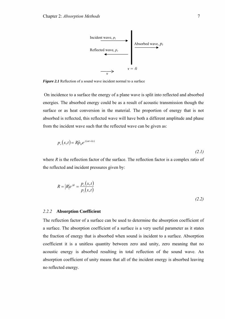
Figure 2.1 Reflection of a sound wave incident normal to a surface
On incidence to a surface the energy of a plane wave is split into reflected and absorbed
energies. The absorbed energy could be as a result of acoustic transmission though the
surface or as heat conversion in the material. The proportion of energy that is not
absorbed is reflected, this reflected wave will have both a different amplitude and phase
from the incident wave such that the reflected wave can be given as:
( ) )(0ˆ, kxtj
r epRtxp += ω
(2.1)
where R is the reflection factor of the surface. The reflection factor is a complex ratio of
the reflected and incident pressures given by:
( )( )txp
txpeRRi
rj
,,
== φ
(2.2)
2.2.2 Absorption Coefficient
The reflection factor of a surface can be used to determine the absorption coefficient of
a surface. The absorption coefficient of a surface is a very useful parameter as it states
the fraction of energy that is absorbed when sound is incident to a surface. Absorption
coefficient it is a unitless quantity between zero and unity, zero meaning that no
acoustic energy is absorbed resulting in total reflection of the sound wave. An
absorption coefficient of unity means that all of the incident energy is absorbed leaving
no reflected energy.

Chapter 2: Absorption Methods 8
To derive the absorption coefficient the intensity of a plane wave is considered as given
by:
cpI
0
2
ρ=
(2.3)
Therefore on reflection, the reflected wave is reduced in intensity by a fraction of |R|2
and consequently the fraction of energy absorbed can be given by 1- |R|2. The
absorption coefficient of a surface is therefore expressed as:
21 R−=α
(2.4)
The absorption coefficient of a material is probably the most widely used quantity when
describing absorbent materials and systems and an absorber’s performance is often
given by a graph of absorption coefficient versus frequency.
2.2.3 Surface Impedance
The surface impedance is a very useful parameter as it is very closely linked to the
physical properties of a surface so it provides clear indication of how the surface
behaves given an incident wave. The surface impedance is given by the ratio of pressure
and the particle velocity normal to the surface:
),(),(
txutxpz =
(2.5)
With the surface at x = 0 the combined pressure and velocity normal to the surface can
be given by:
( )
( ) tj
tj
eRc
ptu
eRptp
ω
ω
ρ−=
+=
1ˆ
),0(
1ˆ),0(
0
0
0
(2.6)

Chapter 2: Absorption Methods 9
The surface impedance becomes:
RRcz
−+
=11
0ρ
(2.7)
Separating the surface impedance into its real and imaginary components reveals
information as to the magnitude of absorption and is resonant characteristics which can
be very useful in analysis.
2.3 Porous Absorbers
When most people think of acoustic absorbers they commonly think of porous
absorbers, this is because there are so many materials that are naturally porous and
consequently absorb sound. Many people, in the pursuit of constructing a home studio
or attempting some rudimentary acoustic treatment of an existing room, will use
common materials such as thick curtains, carpets and sofa’s to control the reverberation
time within the room, these all constitute porous absorbers. Porous absorbers must have
open pores as in Figure 2.2 i.e. pores that can support acoustic propagation where the
orifice is at the surface of the absorber. Porous absorbers can be either granular or
fibrous providing they have these open pores. Granular absorbers can be made from
small pieces of almost any rigid or semi rigid material bound together with glues that do
not block pores. Loose granular materials such as sand also constitute porous absorbers
as the gaps between grains provide a complex path for the acoustic waves to propagate
through, but their loose nature often means they are impractical to use, especially in
room acoustics. An example of a fibrous porous absorbent is mineral wool, made by
spinning molten minerals such as sand and weaving the spun fibres together to form a
complicated structure of pores. This complex pore structure leaves a material that is
highly porous and is commonly used for both acoustic and fire insulation as its open
pores allow restricted airflow through the material thus absorbing sound and also
preventing efficient heat exchange.
When sound propagates in small spaces there are losses in energy, primarily caused by
viscous boundary layer effects, i.e. the friction of the viscous air fluid passing through
the orifice of a small hole/pore. It is this friction that causes viscous and heat losses in
Chapter 2: Absorption Methods 10
porous absorbers making them efficient for room acoustic applications. For a porous
absorber to be effective, it is important that the pores are open rather than closed. The
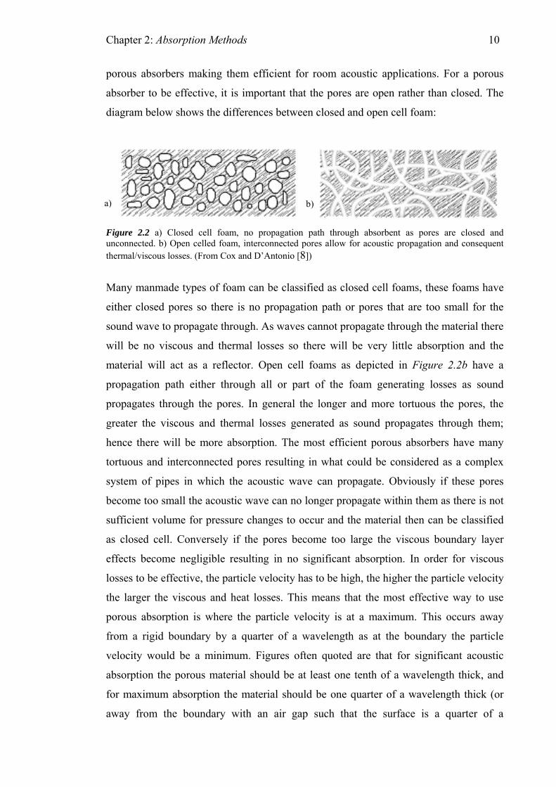
diagram below shows the differences between closed and open cell foam:
a) b)
Figure 2.2 a) Closed cell foam, no propagation path through absorbent as pores are closed and unconnected. b) Open celled foam, interconnected pores allow for acoustic propagation and consequent thermal/viscous losses. (From Cox and D’Antonio [8])
Many manmade types of foam can be classified as closed cell foams, these foams have
either closed pores so there is no propagation path or pores that are too small for the
sound wave to propagate through. As waves cannot propagate through the material there
will be no viscous and thermal losses so there will be very little absorption and the
material will act as a reflector. Open cell foams as depicted in Figure 2.2b have a
propagation path either through all or part of the foam generating losses as sound
propagates through the pores. In general the longer and more tortuous the pores, the
greater the viscous and thermal losses generated as sound propagates through them;
hence there will be more absorption. The most efficient porous absorbers have many
tortuous and interconnected pores resulting in what could be considered as a complex
system of pipes in which the acoustic wave can propagate. Obviously if these pores
become too small the acoustic wave can no longer propagate within them as there is not
sufficient volume for pressure changes to occur and the material then can be classified
as closed cell. Conversely if the pores become too large the viscous boundary layer
effects become negligible resulting in no significant absorption. In order for viscous
losses to be effective, the particle velocity has to be high, the higher the particle velocity
the larger the viscous and heat losses. This means that the most effective way to use
porous absorption is where the particle velocity is at a maximum. This occurs away
from a rigid boundary by a quarter of a wavelength as at the boundary the particle
velocity would be a minimum. Figures often quoted are that for significant acoustic
absorption the porous material should be at least one tenth of a wavelength thick, and
for maximum absorption the material should be one quarter of a wavelength thick (or
away from the boundary with an air gap such that the surface is a quarter of a

Chapter 2: Absorption Methods 11
wavelength from the boundary). With this in mind it becomes clear that as the
wavelength of the incident sound increases, the porous material must increase in depth
if satisfactory absorption is to be achieved. This is the reason that porous absorption is
unsuitable for treating low frequency modal problems in rooms, because the
wavelengths are sufficiently large that much of the room would be taken up by the
porous absorption, which is impractical. An exception to this is in the construction of
anechoic chambers where broadband absorption is needed across the entire audio
spectrum; porous absorption is used here so the absorption coefficient is roughly equal
across a large bandwidth (a useful characteristic of porous absorption). Very thick
porous absorption is used to tackle even the low frequencies in this case as low
frequency resonant absorption would reflect and cause problems at higher frequencies.
2.3.1 Characterising and Modelling Porous Absorbers
It is often important to be able to predict accurately the performance of porous absorbers
both for use on their own and also when used as part of a resonant absorber (see section
2.4). Being able to predict the reverberation time of a room and even to auralise its
response before building or before acoustic treatment is added is becoming increasingly
important in room acoustic design. With the increase in building regulations governing
the acoustic insulation requirements of buildings, it is also imperative that the
absorption characteristics of materials is known before building to ensure the building
will reach the necessary standards on completion. This task is only possible when
accurate information can be given about the absorption within the room. For these
reasons and to aid research into the development of new absorptive materials much
attention has been placed on defining the characteristics of materials and also predicting
their acoustic performance. In order to accurately model porous materials it is important
to determine certain physical properties of the material.
2.3.1.1 Material Properties
The performance of a porous absorber is governed by two main characteristics; the
material’s porosity and flow resistivity. The porosity is the fraction of the amount of air
volume in the absorbent material, it is calculated by the ratio of pore volume to the total
volume of the absorbent material i.e. a porosity of 0.5 means that half of the volume of

Chapter 2: Absorption Methods 12
the material constitutes the air in the pores, the other half (the material that supports the
pore structure) would be the ‘frame’ of the material. Closed pores do not count in
measurements of porosity as they cannot be accessed by incident sound waves and are
therefore ineffective for absorption. Foam with entirely closed pores would have a
porosity of zero.
Flow resistivity is a metric that defines how easily air can enter a material and the
resistance to flow that it experiences as it passes through, analogous to electrical
resistivity. It is a measure of how much energy will be lost due to propagation through
the pores. Flow resistivity can be defined as the resistance to flow per unit thickness of
the material. The viscous resistance to air flow through a porous material causes a
pressure drop across the material which at low frequencies is proportional to the flow
velocity, U and thickness of the material, d. The ratio of this drop in pressure with the
product of the flow velocity and material thickness gives the material’s flow resistivity:
Ud
pΔ=σ
(2.8)
The flow resistance of a material can also be useful and is given by multiplying the flow
resistivity by the material thickness. However flow resistivity is more useful in the
modeling of acoustic materials and is the property used throughout this thesis.
Both porosity and flow resistivity are very important factors but it is the flow resistivity
that varies the most from material to material and therefore is considered the most
important factor. The porosity of an effective porous absorbent is often very close to
unity and varies very little with different materials.
Another factor that will affect the performance of porous absorbers is the tortuousity,
which states how tortuous or ‘wiggly’ the pores of a material are. Tortuosity is basically
a metric of the complexity of the propagation path through the absorbent. A material
with a higher tortuosity will exhibit greater absorption, as a more tortuous path of
propagation makes it harder for the acoustic wave to pass through the material so more
energy is lost through heat as the viscous air fluid is forced through the small pores.
Pore shape is also a factor that influences the amount of absorption from a porous

Chapter 2: Absorption Methods 13
absorber. Pore shape is difficult to define as materials often exhibit many pores with
very different shapes and as such it is a difficult parameter to accurately define.
There are many different strategies for the modeling of porous materials using a variety
of different approaches with varying degrees of complexity and overview of some of
these can be found in [9]. The primary model used in this thesis is a one parameter
empirical approach by Delany and Bazley [10]. In this model the porosity is considered
to be unity and the material parameter needed is the flow resistivity. It is therefore
important that the flow resistivity of the material used is accurately measured; the
following describes the process of this measurement.
2.3.1.1.1 Measuring Flow Resistivity
Flow resistivity can be measured using a relatively simple experimental setup as shown
in Figure 2.3. The premise is to induce airflow through the test sample and to measure
the resulting pressure difference across the sample. Details of this procedure are
outlined in an international standard [11]. The standard outlines two different methods
for the measurement of flow resistivity, the first utilising unidirectional airflow and the
other an alternating airflow. The apparatus chosen here typified an apparatus to measure
flow resistivity using unidirectional laminar flow.
Flow generator
Sample
Laminar flow through sample
Sample holder
Manometer, A Differential pressure gauge, B. Open to atmosphere
Figure 2.3 Test apparatus for measurement of flow resistivity

Chapter 2: Absorption Methods 14
In Figure 2.3 the manometer, A is used to calculate the airflow velocity through the
sample, this is achieved in the test apparatus using the calibration chart for this
particular set up which can be found in Appendix A. From this manometer reading the
volumetric airflow rate, qv can be determined in cubic meters per second. When divided
by area this gives the linear airflow velocity, V. The pressure difference across the
sample with respect to the atmosphere can be deduced from the differential pressure
gauge, B. from these values the specific airflow resistance, Rs can be written as:
Vp
qpAR
vs
Δ=
Δ=
(2.9)
Where is the pressure drop across the sample measured with the differential pressure
gauge, and A is the cross sectional area of the sample. The flow resistivity σ of the
sample is the specific flow resistance per meter:
pΔ
Vdp
dRs Δ
==σ
(2.10)
where d is the depth of the sample.
This gives a measure of flow resistivity which can be used in many acoustic models and
will be used in subsequent sections of this work in a basic one parameter model for rigid
frame porous materials as part of a transfer matrix model presented later.
2.3.1.2 Prediction Models
Attempting to predict the performance of a porous absorber using an analytical
approach is not easy, many models assume that pores are either slits, circular or at least
have a simple geometry but this is rarely the case in reality and consequently models are
fraught with inaccuracies even when many material parameters are considered; as a
result empirical models such as Delany and Bazley [10] have been formulated, which
provide a good basis for modeling porous materials. The Delany and Bazley model is
based on many measurements taken of fibrous porous absorbents. Using curve-fitting
Chapter 2: Absorption Methods 15
techniques they then put an empirical formula together to allow the prediction of both
the characteristic impedance and the complex wavenumber of fibrous absorbent
materials. The formulae assume porosity close to unity and include the material’s flow
resistivity, accurate only between 1000 and 50000 MKS raylm-1. Delany and Bazley’s is
a single parameter model meaning only the material’s flow resistivity is needed for
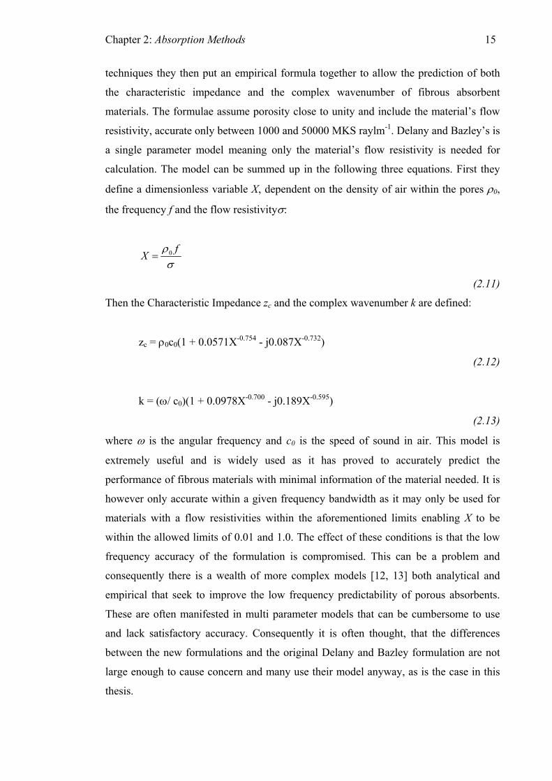
calculation. The model can be summed up in the following three equations. First they
define a dimensionless variable X, dependent on the density of air within the pores ρ0,
the frequency f and the flow resistivityσ:
σρ fX 0=
(2.11)
Then the Characteristic Impedance zc and the complex wavenumber k are defined:
zc = ρ0c0(1 + 0.0571X-0.754 - j0.087X-0.732)
(2.12)
k = (ω/ c0)(1 + 0.0978X-0.700 - j0.189X-0.595)
(2.13)
where ω is the angular frequency and c0 is the speed of sound in air. This model is
extremely useful and is widely used as it has proved to accurately predict the
performance of fibrous materials with minimal information of the material needed. It is
however only accurate within a given frequency bandwidth as it may only be used for
materials with a flow resistivities within the aforementioned limits enabling X to be
within the allowed limits of 0.01 and 1.0. The effect of these conditions is that the low
frequency accuracy of the formulation is compromised. This can be a problem and
consequently there is a wealth of more complex models [12, 13] both analytical and
empirical that seek to improve the low frequency predictability of porous absorbents.
These are often manifested in multi parameter models that can be cumbersome to use
and lack satisfactory accuracy. Consequently it is often thought, that the differences
between the new formulations and the original Delany and Bazley formulation are not
large enough to cause concern and many use their model anyway, as is the case in this
thesis.

Chapter 2: Absorption Methods 16
2.3.1.2.1 Acoustic Impedance Modelling of Multiple Porous Layers
Often important in acoustic modeling and applications is the behaviour of acoustic
waves propagating through layers of different media. This encapsulates many scenarios,
ranging from sound traveling through a porous absorbent mounted on a rigid backing
through to more complicated situations where there are many layers all with different
characteristic impedances and the overall impedance needs to be found. In order to
study accurately the behaviour of sound in these cases a modeling system needs to be
formulated. Considering a wave approach enables a simple model to be put together,
often called a two port model as it has just two ports (both a single input and single
output). This type of model can also be extended to work for more complicated
situations where further resonant layers are introduced (see section 2.4.2.1.1).
Considering plane waves incident only normal to the surface, a diagram of an acoustic
wave incident to a multiple layered absorber can be represented by Figure 2.4:
dx −= 0=x
d pi
pt
pr
Medium A Medium B
x -direction
Figure 2.4 Diagram of sound propagation through multiple layers
At any point the total pressure can be seen as simple addition of the incident, reflected
and transmitted pressures such that:
jkx
rjkx
ijkx
tt epepepxp +== −−)(
(2.14)
So when : 0=x

Chapter 2: Absorption Methods 17
rit ppp +=)0(
(2.15)
Velocity is a vector quantity therefore the addition of the velocities before and after the
boundary of the layer is:
( )ric
rit ppz
uuu −=−=1)0(
(2.16)
where zcis the characteristic impedance of material A.
From equations 2.14 and 2.15, the incident and reflected pressures at the boundary
can be expressed as: 0=x
ctir
ctri
zuppzupp
)0()0(
−=+=
(2.17)
Therefore:
( )
( )cttr
ctti
zupp
zupp
)0()0(21
)0()0(21
−=
+=
(2.18)
So the sound pressure at any point x in space (assuming normal incidence) can be given
by equation 2.19:
( ) ( ) jkxctt
jkxctt
jkxr
jkxi
jkx ezupezupepeppexp )0()0(21)0()0(
21)( −++=+== −−−
(2.19)
Expanding this gives the transmitted pressure as:

Chapter 2: Absorption Methods 18
( )( )
( )(
)sin()0()cos()0()(
sin()cos()0()0(21
...sin()cos()0()0(21)(
kxjuzkxpepxp
kxjkxzup
kxjkxzupepxp
tctjkx
tt
ctt
cttjkx
tt
−==
⎥⎦⎤
⎢⎣⎡ +−
+⎥⎦⎤
⎢⎣⎡ −+==
−
−
)
(2.20)
And the transmitted velocity as:
( ) ( ) ( )
)sin(1)cos()(
21
2111)(
kxjpz
kxueuxu
ezupezupz
epepZc
euxu
tc
tjkx
tt
jkxctt
jkxctt
c
jkxr
jkxi
jkxtt
−==
⎥⎦⎤
⎢⎣⎡ −++=−==
−
−−−
(2.21)
The ratio of the transmitted pressure and velocity at a point x gives the acoustic
impedance at that point. So in order to find the impedance at the boundary of material A,
. Substituting this into the above equations gives: dx −=
2
2
( ) (0)cos( ) (0)sin( )( )( ) (0)cos( ) (0)sin( )
(0) cot( ) (0)(0) cot( ) (0)
(0) cot( )(0) cot( )
t t c tt
tt t
c
t c c t
t c t
t c c
t t c
p d p kd jz u kdz d ju d u kd p kz
jp z kd z uju z kd p
jz z kd zz jz z kd
− +− = =
− +
− +=
− +
− +=
−
d
(2.22)
Where zt is the surface impedance at 0=x (termination impedance) given by pt(0)/ut(0),
zc is the characteristic impedance of the layer with thickness d. zt(-d) is the surface
impedance at the point dx −= . k is the wavenumber in the material, this can often be
determined by a simple empirical model for porous absorbents or as 2 cf /π if in air.
Equation 2.22 can be used in any general case as long as the wavenumber within and
characteristic impedance of the materials are known. It can also be written in matrix
form which as part of a transfer matrix [14] as represented by equation 2.32:

Chapter 2: Absorption Methods 19
2.4 Resonant Absorption
Unlike porous absorption, which is used primarily for absorption of mid to high
frequency sound, resonant absorption is most commonly used for treating low
frequency acoustic problems. Resonant absorption is sometimes used for higher
frequency applications where porous absorbers are impractical i.e. where weather or
fumes could damage or clog the pores. It is however not common to use resonant
absorption for higher frequency problems because the bandwidth of absorption is
commonly a lot lower than porous absorption if high absorption coefficients are to be
achieved. This narrow bandwidth corresponds to a very small fraction of an octave band
at higher frequencies so is often considered impractical.
Resonant absorbers are essentially mass-spring systems where sound pressure incident
on the absorber causes a mass element to vibrate on a spring which is damped to
introduce energy loss and consequently absorption. Resonant absorbers are most
efficient if placed in areas where acoustic pressures are high, as higher pressures induce
greater movement of the mass. As a result, resonant absorbers are often placed on the
boundaries of a room and often in the corners where room modes have maximum
pressure amplitude so maximally efficient absorption can be achieved. This contrasts
with porous absorbers, which are most effective in areas of maximum particle velocity
i.e. away from boundaries.
There are two main types of resonant absorption, namely Helmholtz absorbers named
after Hermmann Von Helmholtz (1821-1894) and membrane absorbers. Both are
commonly used in room applications and also as silencers in engines and ventilation
ducts et cetera. Theory of both techniques is presented in the following sections.
2.4.1 Helmholtz Absorbers
Helmholtz absorbers consist of a plate with many holes equally spaced in both the x and
y plane, which are usually damped with porous absorption, unless the holes are
sufficiently small as to generate absorption without it. The resonating mass is the plug
of air that is in the holes and the spring is the air compliance of the volume between the
front and back plates. Figure 2.5 shows the construction of a typical Helmholtz
absorber:

Chapter 2: Absorption Methods 20
Resonant air flow through perforations D
Figure 2.5 Schematic representation of a typical Helmholtz absorber
Both membrane and Helmholtz resonant absorption attempt to convert areas of high
acoustic pressure into a region of high particle velocity that can be absorbed by
intelligently positioned porous absorption. In the case of a Helmholtz absorber, incident
pressure causes highest particle velocity in the neck of each orifice so porous materials
are often placed there to maximise absorption efficiency, in practical applications
however the porous absorbent is usually placed in between the two plates for ease of
manufacture and cost efficiency.
2.4.1.1 Predicting the Performance of Helmholtz Absorbers
The performance and resonant frequency of Helmholtz absorbers is easy to predict and
can be done to a high degree of accuracy by considering each orifice to be a short tube
forming individual Helmholtz resonators as shown in Figure 2.6:
Figure 2.6 Diagram of a Helmholtz type acoustic resonator
Porous AbsorbentSealed enclosure
Perforated sheet
2a
t
d
dDV 2=
2aS π= t
Chapter 2: Absorption Methods 21
A short tube terminated with a low impedance behaves like an inert mass, [7] therefore
the acoustic mass per unit area of the Helmholtz absorber is given by equation 2.23
assuming the geometry given in Figure 2.5:
ερ
πρ t
atD
m 02
20 ==
(2.23)
where 2
2
Daπε = and is termed the fractional open area or ‘porosity’ of the perforated
sheet.
Each plug of air is considered to behave like a baffled piston such that it is subject to a
radiation impedance given by equation 5.19, [15]. The value of this radiation impedance
depends on whether or not the holes are flanged. Considering a flanged termination
introduces an end correction as a result of the radiation impedance which adds an
apparent extra length of aa 85.03/8 ≈π to each end of the plug of air thus equation 2.23
becomes:
ερ
ερ ')7.1( 00 tatm =
+=
(2.24)
where is the apparent length of each plug as a result of end corrections. The
mechanical impedance of a Helmholtz resonator is the sum of the impedance due to
radiation resistance Rr, stiffness K, and mass per unit area m, such that:
t ′
rM RjKmjZ ++=ω
ω
(2.25)
Considering just one plug, ε becomes unity and the stiffness of the plug can be
expressed as [15]:
VScK
22
0ρ=
(2.26)

Chapter 2: Absorption Methods 22
The resonant frequency can therefore be determined by setting the imaginary part to
zero. The resonant frequency can then be found by:
( )
'2'2
'/
21
0
0
220
0
dtc
VtScf
tVsc
f
εππ
ρρ
π
==
=
(2.27)
To formulate the absorption of a Helmholtz absorber it is possible to define a lumped
element model as in chapter 5, it is often more helpful however to consider in the entire
acoustic system as a combination of layers as part of a transfer matrix model (see
section 2.4.2.1.1). In this case the impedance of the perforated sheet is simply added
onto the impedance of the backing to find the overall impedance; from here the
absorption coefficient can easily be found from equations 2.7 and 2.4.
2.4.2 Membrane Absorbers
Membrane or panel absorbers are also mass-spring systems, this time however the
vibrating mass is a flexible membrane or plate and the spring is the compliance of the
sealed air cavity of the box backing the membrane. A standard design of membrane
absorber is shown below:
Porous Absorbent
Particle velocity v
Movement of membraneSmall gap to allow free movement of membrane/panel
Enclosure, with compliance C
Flexible membrane/panel Mass/unit area m
Figure 2.7 Schematic representation of a standard membrane absorber
High pressure acoustic waves meeting the surface of a membrane cause it to oscillate at
a frequency governed by its mass, and the stiffness of the air spring of the cavity. The
air spring is considered linear as long as there are no standing waves in the cavity within
Chapter 2: Absorption Methods 23
the fundamental frequency range, which is almost always the case with membrane
absorbers. The vibration of the membrane creates high particle velocities at its rear that
effectively force air through the porous absorbent thus generating high levels of
absorption. This however is only over a limited bandwidth i.e. the resonance peak of
absorption has a high Q-factor. The bandwidth can be increased by increasing the
damping, but as with any mass-spring system, this has the effect of decreasing the
maximum efficiency of the absorber. A trade off therefore ensues between bandwidth
and maximum absorption.
Unlike Helmholtz absorbers, prediction of the behavior of membrane absorbers is
difficult and often inaccurate this is because the exact mounting conditions and
properties of the membrane are hard to predict and model. Not being able to model the
mounting conditions accurately is problematic as membrane absorbers often exhibit
losses and hence absorption from the edges. Many common formulations also assume
that the membrane cannot support higher order modes than the fundamental resonant
frequency i.e. they assume that the membrane moves as a lumped mass system in much
the same way as a piston does. These simpler models do not allow for the membrane to
support bending waves and consequently don’t result in accurate predictions especially
at oblique incidence, when bending waves are more easily excited.
2.4.2.1 Predicting the Performance of Membrane Absorbers
If the membrane is considered to oscillate as a piston and its bending stiffness is ignored
such that the restoring force is entirely due to the compliance per unit area C of the air
volume where:
20cdC
ρ=
(2.28)
An equation of the impedance of the cavity backed membrane can then be written as:
MRC
MjZ +⎟⎠⎞
⎜⎝⎛ −=
ωω 1
(2.29)

Chapter 2: Absorption Methods 24
where M is the mass per unit area of the membrane or plate and RM is the mechanical
losses of the mounting. The resonant frequency of this system can be found by setting
the imaginary part to zero thus:
21
20
0 ⎟⎟⎠
⎞⎜⎜⎝
⎛=
Mdcρ
ω , so Md
f 600 ≈
(2.30)
Equation 2.30 is a useful first approximation but it only defines the condition with an
empty cavity. If the cavity contains porous absorbent as is common in the design of
such absorbers the resonant frequencies predicted by this formula tend to be too high.
This formula can therefore be altered to account for the adiabatic case as [7]:
Mdf 50
0 =
(2.31)
These provide a useful first approximation but often yield inaccurate results with errors
of up to 10 per cent. This inaccuracy is largely because the mechanical properties of the
panel are not taken into account. With the edges of the panel fixed its bending stiffness
will, especially for thicker panels, contribute considerably to the restoring force of the
system such that it cannot be approximated simply by equation 2.28. Accurately
predicting this bending stiffness is particularly difficult especially when the exact
boundary conditions of the membrane or plate are uncertain.
16,17Other formulations and methods are also often used [ ], these techniques have the
disadvantage of being complex and need extensive knowledge of the material properties
to be accurate. However even with accurate determination of these properties
assumptions are still made for the mounting conditions which are often inaccurate,
leading to errors in the predicted performance. A more simplistic method for prediction
of resonant absorbers is the transfer matrix method which builds upon the theory of
sound traveling through different layers of porous media mentioned in section 2.3.1.2.1.
This technique is often thought better as it is adaptable for many scenarios of
construction and yields results with reasonable accuracy.

Chapter 2: Absorption Methods 25
2.4.2.1.1 Transfer Matrix Modelling
The transfer matrix approach is a very useful tool as it allows surface velocities,
pressures to be calculated this enables the more useful determination of the surface
impedance.
Writing equation 2.22 in matrix form gives the pressure and velocity at a point x as:
⎭⎬⎫
⎩⎨⎧
⎪⎭
⎪⎬⎫
⎪⎩
⎪⎨⎧
=⎭⎬⎫
⎩⎨⎧
)0()0(
)cos()sin(
)sin()cos(
)()(
t
t
c
c
t
t
up
kdkdzj
kdjzkd
xuxp
(2.32)
This is part of a transfer matrix that can be found in Allard [14]. The transfer matrix
method uses the surface impedance of one layer as the backing impedance of the next
enabling any number of layers to be combined and the final surface impedance found. It
is a very useful tool for designing absorbers as it eliminates the need for iterative
development which is both costly and time consuming in the design of absorber
systems. The transfer matrix method allows many different systems to be predicted
ranging from the simple case of a porous material mounted on a rigid wall up to
multiple porous layers including membrane and Helmholtz layers. In order to perform
calculations, the characteristic impedance of the material of each layer must be known.
This can be achieved easily in many cases such that a porous layer can be represented
by empirical or semi-empirical formulations like the Delany and Bazley model as
mentioned in section 2.3.1.1. The characteristic impedance of membrane and Helmholtz
layers can be more problematic to predict with accuracy as often boundary conditions
are not known and as such approximations have to be made. For the membrane case the
membrane is assumed to be very thin such that there are no bending waves present. It is
thereby assumed to move as a pistonic mass. The impedance in this case can be
considered as a series combination (that is the simple addition) of a single resistive and
reactive term. In general membranes are assumed to move pistonically with a nominal
resistance to motion made up from the mounting and resistive losses in the material.
The impedance therefore is given by equation 2.35.
Assuming that only plane waves are incident on the multi-layered absorber system and
only considering propagation in the x and y direction, the propagation through the

Chapter 2: Absorption Methods 26
system can be represented by Figure 2.8. The initial case is considered with a
membrane mounted on a cabinet filled with absorbent material.
Figure 2.8 Diagrammatic representation of the transfer matrix modeling of sound incident to a membrane
absorber
The equation that links all of the surface pressures and velocities and allows hence the
calculation of the surface impedance is the same as in section 2.3.1.2.1 but with
different notation equation 2.22 can therefore be written as:
( )( )iiisi
iiiisisi dkjzz
zdkzjzzcot
cot 2
1 −+−
=+
(2.33)
rp
ip
(i+1)th layer ith layer (i-1)th layer
1
1
−
−
i
i
zk
tp
2rp 2tp
MR di
Assume rigid backing:
i
i
zk
∞=∴ −1iz and
02 =tp
Membrane, mass/unit area, assumed to move as a piston such that its reactance,
MM
j MM MX ω=
Resistive losses, due to mounting of m
MR
embrane
pxi+1 uxi+1
px
i ux
i
xi+1 xi-1 xi zsi+1 zsi
y
x

Chapter 2: Absorption Methods 27
Using this notation it easier to keep track of multiple layered systems. Applying this to
the ith layer, the backing is considered to have infinite impedance such that ∞≈siz and
the above equation simplifies to:
)cot(1 iiisi dkjzz −=+
(2.34)
Where ki can be determined from a model for porous media such as Delany and Bazley
and di is the depth of the porous material. This value can then be used as zsi for the next
layer and the impedance calculated for further layers of materials. From this the
absorption coefficient can be calculated and plotted against frequency yielding the
standard result for mineral wool as shown in Figure 2.9:
1
0 50 100 150 200 250 300 350 400 450
0.9
0.8
0.7
0.6
0.5
0.4
0.3
0.2
0.1
5000
Frequency, Hz
Abs
orpt
ion
Coe
ffici
ent
Transfer Matrix Model Using Delany and Bazley Prediction
Mineral Wool 10cm Deep on a Rigid Backing
Figure 2.9 Transfer matrix modeling of porous absorbent with a rigid backing using the Delany and
Bazley model
When adding a membrane to the front of the absorber system the impedances work in
series with each other such that the overall impedance can be determined simply by the
addition of the resistive and reactive impedances of the membrane:
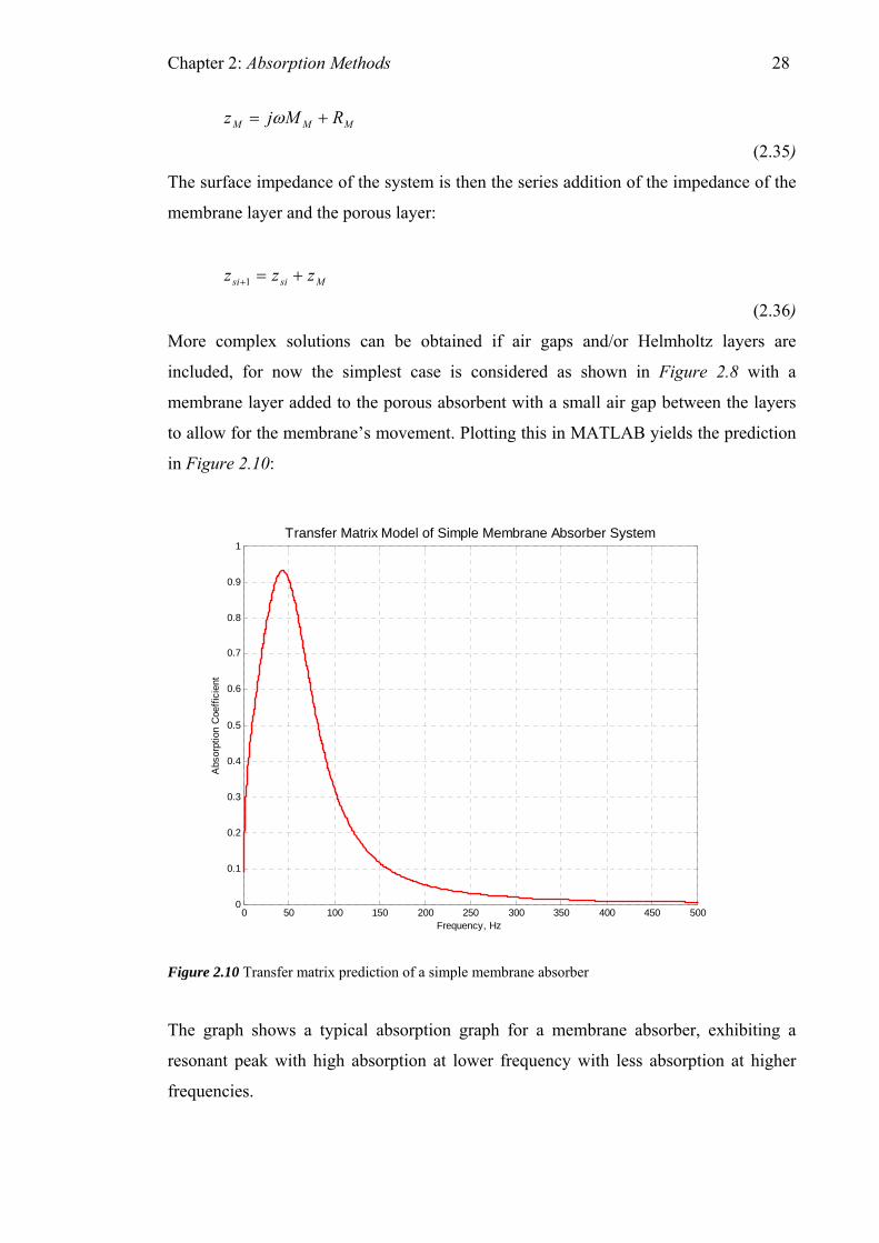
Chapter 2: Absorption Methods 28
MMM RMjz += ω
(2.35)
The surface impedance of the system is then the series addition of the impedance of the
membrane layer and the porous layer:
Msisi zzz +=+1
(2.36)
More complex solutions can be obtained if air gaps and/or Helmholtz layers are
included, for now the simplest case is considered as shown in Figure 2.8 with a
membrane layer added to the porous absorbent with a small air gap between the layers
to allow for the membrane’s movement. Plotting this in MATLAB yields the prediction
in Figure 2.10:
1
0 50 100 150 200 250 300 350 400 450
0.9
0.8
0.7
0.6
0.5
0.4
0.3
0.2
0.1
0500
Frequency, Hz
Abs
orpt
ion
Coe
ffici
ent
Transfer Matrix Model of Simple Membrane Absorber System
Figure 2.10 Transfer matrix prediction of a simple membrane absorber
The graph shows a typical absorption graph for a membrane absorber, exhibiting a
resonant peak with high absorption at lower frequency with less absorption at higher
frequencies.

Chapter 2: Absorption Methods 29
The predictions so far have dealt only with waves incident normal to the surface of an
absorber, this is a useful case and matches closely to the testing of an absorber in an
impedance tube and therefore is very useful for comparison of predictions and
measurements. There is however scope for extending the transfer matrix approach for
oblique incidence waves by considering the wavenumber in materials as a vector
quantity with components in the x and y direction. Such that:
222
yx kk +=k
(2.37)
Using Snell’s law it is then possible to define the refractive effect as the acoustic waves
propagate through each medium. The equation then becomes:
( )
( )ixixi
isi
xi
iiixi
xi
iisi
si
dkkkijzz
kkzdk
kkzjz
zcot
cot2
1
−
⎟⎟⎠
⎞⎜⎜⎝
⎛+−
=+
(2.38)
For most porous absorbents the x component of the wavenumber vector, k is equal to
the scalar wavenumber in that material as the angle of incidence tends to the normal.
Thus often the angle of incidence is not needed. For the purposes of this project only
normal incidence will be modeled.
2.5 Conclusion
It has been seen how both porous materials and damped acoustic resonators can be used
in the field of room acoustics to absorb sound in high and low frequency bands. Theory
of these methods has been outlined along with the relevant prediction models that will
be used in subsequent sections of this work. The theory presented in this chapter will
serve as a useful background to the analysis, modeling and development of more
complicated absorber systems presented in chapters 4, 5 and 6.
Chapter 3: Measuring Absorption Coefficient and Surface Impedance 30
3. MEASURING ABSORPTION
COEFFICIENT AND SURFACE
IMPEDANCE
3.1 Introduction
The previous chapter outlined some theory and prediction techniques for the
performance of acoustic absorbers. This chapter describes and demonstrates some
useful techniques for the measurement of absorption characteristics. Of primary interest
is the surface impedance of an absorber, be it porous or resonant. From this quantity, the
reflection factor and the absorption coefficient can be found giving a good idea of the
absorber’s performance with respect to frequency.
Two main methods are used for measuring these absorber characteristics, namely the
reverberation room method and impedance tube method. The former, measures random
incidence absorption coefficient and the latter, the normal incidence absorption
coefficient and surface impedance. In general, the reverberation chamber method is

Chapter 3: Measuring Absorption Coefficient and Surface Impedance 31
used to test larger areas of absorbers such as carpets where samples with large surface
area can easily be obtained. Impedance tubes require much smaller samples and are
often used when developing new absorbers as small samples are more cost effective to
produce. The normal incidence absorption coefficient measured in this case is also
easier to compare with theoretical models than the random incidence absorption
coefficient which is very difficult to predict so is less useful for comparisons.
Both techniques are presented in this chapter along with the design, construction and
commissioning of a low frequency impedance tube especially designed for the
measurement of low frequency absorbers. The cross sectional area of the tube was such
that the entire membrane absorber could fit into it thus allowing accurate testing of its
normal incidence absorption coefficient.
3.2 Reverberation Chamber Method
The basic premise of the reverberation method is to determine how much difference an
absorber makes to the reverberation time in a room, and therefore to determine the
absorption coefficient of the material that would result in this difference. The
reverberation time is measured before and after the addition of the absorption and from
this, the absorption coefficient is derived. The reverberation chamber method is based
on Sabine’s equation for the reverberation time in a room [18]:
cAVT 3.55
=
(3.1)
Where T is the time for the noise source within the room to decay by 60dB from a
steady level, V is the volume of the room, c is the speed of sound and A is the total
absorption area of all surfaces. Rearranging this formula and adding a term for the
absorption due to the air (this becomes significant for larger rooms) gives an equation
for the equivalent sound absorption area of the empty reverberation room, A1:
11
1 43.55 mcT
VA −=
(3.2)
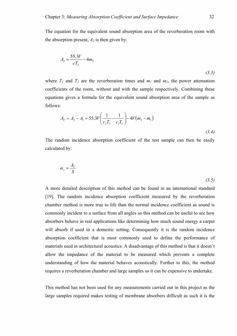
Chapter 3: Measuring Absorption Coefficient and Surface Impedance 32
The equation for the equivalent sound absorption area of the reverberation room with
the absorption present, A2 is then given by:
22
2 43.55 mcT
VA −=
(3.3)
where T1 and T2 are the reverberation times and m1 and m2, the power attenuation
coefficients of the room, without and with the sample respectively. Combining these
equations gives a formula for the equivalent sound absorption area of the sample as
follows:
( )121122
12 4113.55 mmVTcTc
VAAAT −−⎟⎟⎠
⎞⎜⎜⎝
⎛−=−=
(3.4)
The random incidence absorption coefficient of the test sample can then be easily
calculated by:
SAT
s =α
(3.5)
A more detailed description of this method can be found in an international standard
[19]. The random incidence absorption coefficient measured by the reverberation
chamber method is more true to life than the normal incidence coefficient as sound is
commonly incident to a surface from all angles so this method can be useful to see how
absorbers behave in real applications like determining how much sound energy a carpet
will absorb if used in a domestic setting. Consequently it is the random incidence
absorption coefficient that is most commonly used to define the performance of
materials used in architectural acoustics. A disadvantage of this method is that it doesn’t
allow the impedance of the material to be measured which prevents a complete
understanding of how the material behaves acoustically. Further to this, the method
requires a reverberation chamber and large samples so it can be expensive to undertake.
This method has not been used for any measurements carried out in this project as the
large samples required makes testing of membrane absorbers difficult as such it is the

Chapter 3: Measuring Absorption Coefficient and Surface Impedance 33
impedance tube method outlined in section 3.3 that is used for measurements
throughout this work.
3.3 Impedance Tube Method
Impedance tubes offer a more controlled test environment and have the advantage over
the reverberation method that they enable the measurement of the acoustic impedance of
a sample or system. Impedance tubes are cheaper to use than the reverberation chamber
technique because less specialist equipment is needed; also the sample sizes can be
much smaller, cutting down on waste. There are two techniques for using impedance
tube; the standing wave method and the transfer function or ‘two-microphone method’.
Both methods are outlined below and can also be found in the relevant International
Standards [20, 21]. Brief theory of both methods is given below.
3.3.1 Standing Wave Method
The standing wave method was the earliest method devised for measuring absorption using a tube it evolved from August Kundt’s (1839-1894) tube for measuring the speed of sound and is simpler in principle than the transfer function approach. The basic premise is as follows. Plane waves propagate down the tube from the loudspeaker and are reflected from the other end of the tube where the sample is mounted, consequently setting up standing waves in the tube. Measuring the relative amplitudes of the maxima and minima of the standing waves using a moving probe microphone enables the absorption coefficient to be calculated, for discrete frequencies. A diagram showing the construction and operation of a standing wave tube is shown in Figure 3.1:
Figure 3.1 Diagram of the typical setup of an impedance tube using the standing wave method
With the loudspeaker source on, a standing wave will be set up in the tube. The probe
microphone can be moved up and down the tube in order to find the first pressure
maximum and the first pressure minimum from the sample. This can be done by simply
connecting the output from the microphone to a voltmeter. Noting down the values and
Rigid Termination
Probe Tube
Microphone
Trolley
Loudspeaker
Sample
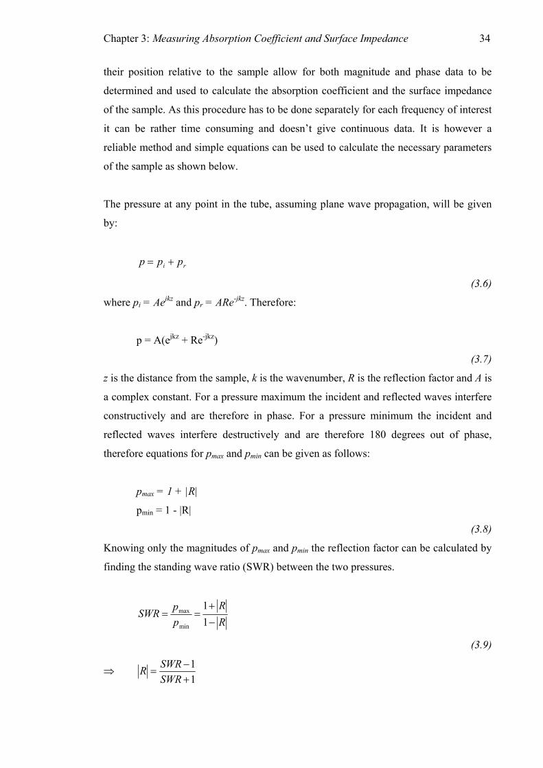
Chapter 3: Measuring Absorption Coefficient and Surface Impedance 34
their position relative to the sample allow for both magnitude and phase data to be
determined and used to calculate the absorption coefficient and the surface impedance
of the sample. As this procedure has to be done separately for each frequency of interest
it can be rather time consuming and doesn’t give continuous data. It is however a
reliable method and simple equations can be used to calculate the necessary parameters
of the sample as shown below.
The pressure at any point in the tube, assuming plane wave propagation, will be given
by:
ri ppp +=
(3.6)
where pi = Aejkz and pr = ARe-jkz. Therefore:
p = A(ejkz + Re-jkz)
(3.7)
z is the distance from the sample, k is the wavenumber, R is the reflection factor and A is
a complex constant. For a pressure maximum the incident and reflected waves interfere
constructively and are therefore in phase. For a pressure minimum the incident and
reflected waves interfere destructively and are therefore 180 degrees out of phase,
therefore equations for pmax and pmin can be given as follows:
pmax = 1 + |R|
pmin = 1 - |R|
(3.8)
Knowing only the magnitudes of pmax and pmin the reflection factor can be calculated by
finding the standing wave ratio (SWR) between the two pressures.
RR
ppSWR
−+
==11
min
max
(3.9)
⇒ 11
+−
=SWRSWRR

Chapter 3: Measuring Absorption Coefficient and Surface Impedance 35
(3.10)
From this, the absorption coefficient of the sample can be found using equation 2.4.
If the surface impedance is wanted then the position of the first minimum can be noted
and used in equation 3.11 to calculate the argument of R which can then be used to
derive the surface impedance of the sample:
( ) nkZn min,212 =−+ πφ
(3.11) φjeRR =
(3.12)
Here n is the number of the pressure minimum measured. From this the complex
impedance is given by:
RRcZ
−+
=11
0ρ
(3.13)
Although this method does allow for any of the pressure minimums to be measured it is
better to use only the first minima as this will eliminate effects from losses in the tube
walls.
Calibration isn’t necessary for the standing wave method because pressure values have a
constant offset, which appears in the complex amplitude, A, and cancels out in the
pressure ratio. This makes things simpler and results in an easy method for measuring
absorption of samples.
There is a low frequency limit of a standing wave tube, which is governed by its length
i.e. ensuring that a maximum and a minimum can be found. The standard dictates that at
least two minima should be able to be found, this imposes a low frequency limit on the
tube of:
lcfl
75.0=

Chapter 3: Measuring Absorption Coefficient and Surface Impedance 36
(3.14)
Where l is the length of the tube and c is the wave speed in the tube.
The standing wave method is more reliable and failsafe than the transfer function
method mentioned in section 3.3.2 but it is rather tedious as it can be time consuming to
locate and measure the positions of the minima in order to obtain the phase data, and to
do this for each frequency of interest.
3.3.2 Transfer Function Method
This method is often thought superior to the standing wave method because it allows all frequencies to be calculated simultaneously thereby producing continuous data in the frequency domain with just two measurements. As such, this method is less time consuming and can be easier to verify results with predictions. Figure 3.2 shows a diagram of a typical setup of a transfer function impedance tube:
Sample
z1
Rigid Termination z2
Loudspeaker Microphone 2 Microphone 1
Figure 3.2 Diagram of the typical setup of an impedance tube using the transfer function method
The transfer function method operates within a certain frequency range, depending on
the microphone positions and diameter of the tube governed by equations 3.17, 3.18 and
3.19. The lower of the two upper frequency limits should be chosen so that both
equations are satisfied. Although often called the ‘two microphone method’ (as it uses
at least two microphone positions) the transfer function method is a better name as it
describes the process by which the results can be obtained.
The steady state pressure at a point in the tube is given by equation 3.7 where units and
symbols have their usual meanings, z being the distance from the sample to the
microphone. There are two unknowns in this equation namely the magnitude and the
phase of the complex reflection factor. The two microphone positions are used to get

Chapter 3: Measuring Absorption Coefficient and Surface Impedance 37
two pressure equations that can be solved simultaneously in order to obtain the two
unknowns. Taking the transfer function of these two pressures gives:
( )( ) 11
22
11
22
.
...
1
212 jkzjkz
jkzjkz
jkzjkz
jkzjkz
eReeRe
eReAeReA
ppH
−
−
−
−
++=
++==
(3.15)
Therefore:
12
21
jkzjkz
jkzjkz
HeeeHeR −− −
−=
(3.16)
From this the impedance and hence the absorption coefficient can easily be derived,
using equations 2.7 and 2.4 respectively.
There are frequency limitations imposed on this method as a consequence of the
microphone positions. If the microphones are too close together the pressure difference
between them is too small to be accurately measured and the method breaks down, the
low frequency limit is usually given by the following equation:
21
05.0zzcfl −
>
(3.17)
If the microphones are too far apart this leads to an upper frequency limit. As the
distance between the microphones becomes equal to a wavelength the pressures at the
two microphones will be the same at the corresponding frequency and the simultaneous
equations will not be solvable. The upper frequency limit imposed by this is therefore
given by:
21
45.0zzcfu −
>
(3.18)
Both of these upper and lower limits are dictated by the microphone positions, hence
often additional microphone positions are used in order to increase the useable
frequency range of this method, computing the transfer function separately for each pair
of microphone positions.
Chapter 3: Measuring Absorption Coefficient and Surface Impedance 38
Microphones cannot be placed too near to the sample or to the source to ensure accurate
easurements. The first microphone should be at least two tube diameters from the
er function method it is common to use a deterministic
oise source such as a swept sine wave or an MLS noise source [22] rather than simply
m of the microphone should always be flush with the side of the tube and
ealed, to enable accurate results. Of utmost importance is that the unused hole be
.3.3 General Considerations for Impedance Tube Testing
Whichever impedance tube method is being used, some important general principles
mple and tube walls is
m
loudspeaker as by this point any cross modes that have been generated by the
loudspeaker will have died away and only plane waves will be incident on the sample,
enabling the normal incidence absorption coefficient to be accurately measured.
Subsequent microphones should be sufficiently far from the sample (usually by about ½
diameter of the tube) this is so that any cross modes generated from the reflection of the
sample will have also died away. This tends to be more of a problem for anisotropic
materials so often greater distances are needed between sample and microphone when
these materials are being tested.
Practically, when using the transf
n
white noise. This eliminates the need for phase-matched microphones, which would
otherwise be needed; these can be expensive and would have o be changed over
anyway to verify each measurement for repeatability checking. With a deterministic
signal a measurement can be made at one microphone position, the microphone moved
and the pressure taken at the second position enabling the transfer function to be
calculated.
The diaphrag
t
s
blocked, with the rubber bung or block being flush with the edge of the tube as these
holes can lead to additional absorption due to a Helmholtz effect.
3
need to be applied. It is imperative that a good seal between sa
achieved to prevent extra absorption generated by sound propagating in the small gap or
as a result of a Helmholtz resonance if there is a cavity behind the gap. When mounting
the sample it is also very important to get rid of any unwanted air gaps at the rear of the
sample as these can lead to an increase in low frequency absorption which, if not

Chapter 3: Measuring Absorption Coefficient and Surface Impedance 39
intended, could produce misleading results. Samples should also not be squashed into
the tube as the squashing alters the mechanical properties of the sample i.e. the density
could be altered or additional irregularities in the face of the sample could result,
leading to erroneous results. The sample end of the tube should provide a rigid backing
of impedance approaching infinity without a sample in place such that only the
performance of the sample is tested rather than the combined effect of the absorber and
backing.
Losses in the tube need to be minimized, especially for the standing wave method to
nsure it is only the effect of the sample that is measured rather than of the tube. A
ube,
overned by the first cross modal frequency of the tube such that:
e
constant cross sectional area down the tube, especially near to the sample, is also
required so that only plane waves are incident normal to the surface of the sample.
The diameter of the tube will impose further frequency limits on use of the t
g
dcf = u 2
(3.19)
Where d is the diam
being used. Therefore if low frequency measurements need to be made larger tub
mmissioning of a Low Frequency Impedance Tube
or the purposes of this project it was decided that tests would be carried out in an
eter or maximum width of the tube if a square cross section tube is
es will
be needed, this is the case for testing membrane absorbers such as in this project as they
are not scalable, for this reason a larger impedance tube was constructed, the design and
construction of which can be found in the section 3.4. The membrane absorber in this
case had to be designed to fit the diameter of the tube as membrane absorbers are
extended reactors therefore the whole sample had to be measured, taking a small section
of a membrane absorber would not work as the mounting conditions are so key in the
performance of these absorbers.
3.4 The Design, Build and Co
F
impedance tube rather than in the reverberation chamber due to ease of testing and the
need for just one absorber to be constructed for accurate tests. Of course this only gives
the normal incidence absorption coefficient, however after development in the

Chapter 3: Measuring Absorption Coefficient and Surface Impedance 40
impedance tube the absorber systems could be tested in a reverberation room to obtain
data on the random incidence absorption coefficient if desired.
Impedance tubes tend to be designed to such dimensions that they can be used for
sting samples in the mid frequency band. In order to enable the low frequency
.4.1 Design
Using an impedance tube to measure the absorption of a membrane absorber presents a
hat must be overcome in the design stage to prevent experimental
te
performance of membrane absorbers as in this project a larger tube was commissioned.
This section outlines the design, construction and commissioning of a specially built
low frequency impedance tube used for the testing in this project.
3
few problems t
inaccuracies and flawed testing. A membrane absorber is an extended reactor, meaning
that a small section will not behave in a manner that is representative of the entire
system, so sampling a small section of the absorber for testing will not yield good
results as it would for most porous absorbers. For this reason the impedance tube had to
be made to such dimensions that the membrane in question would fit within the inner
walls of the tube, allowing the entire membrane to be tested. A further problem was the
frequency limitations of the tube dictated by its dimensions as outlined by equations
3.17, 3.18 and 3.19. This meant that for satisfactorily low frequency performance
certain dimensions were imposed upon the construction. For both the purposes of this
project and for subsequent projects involving low frequency absorption the tube’s
dimensions were chosen to enable the accurate measurement to the lower limit of the
human auditory range, the lowest measurable frequency of the tube was therefore
designed to be 16Hz. The transfer function method was chosen as this provides ease of
measurement and also gives results for a continuous frequency spectrum. In order to
improve the measurable bandwidth of the tube dictated by the microphone positions,
four microphone holes were made allowing six different microphone pairings. This also
enabled accuracy of results to be checked as the frequency limits of each position
overlap allowing tests of continuity for the overlapping frequency regions. A schematic
of the tube’s design is shown in Figure 3.3 with the relevant dimensions labeled as well
as a photograph of the completed tube. The tube was designed in an upright position

Chapter 3: Measuring Absorption Coefficient and Surface Impedance 41
both for economy of space and also to allow the testing of granular materials for other
projects.
1.226m
Figure 3.3 a) Photograph of complete
3.4.2 Construction
ted from 22mm thick mild steel, this provided enough mass to
d impedance tube b) Schematic of completed impedance tube
The tube was construc
significantly reduce losses from the walls of the tube even at the low frequency end of
the measurement bandwidth. The raw materials were ordered from a local steel
merchant and the manufacture performed onsite at The University of Salford. The
impedance tube consists of four sections of steel, two making up the main chamber and
a further two sections to be used as sample holders (a large one and a smaller one)
allowing for different testing conditions i.e. absorbers with different backing volumes.
The sample holder is placed on the trolley and then jacked into place using the bottle
0.184m
0.368m
0.914m
0.3m Large Sample
2m
Mineral Wool
Bottle Jack
Sample
22mm thick
Mic B
Mic C
Mic D
mild steel
0.346m
Mic A Holder
Holder
0.1m
Small Sa ple Hold
mer
Supporting trolley

Chapter 3: Measuring Absorption Coefficient and Surface Impedance 42
jack to allow for a very tight fit, ensuring no small cracks for leaks between the sections
of tubing. Holes were drilled using a magnetic pillar drill in the positions as outlined
above. Annular rings were welded onto the side of one of the sections of the tube to
prevent the sections from coming apart. Further pieces, also welded on, were used to
support the tube on a stand made from rolled steel joists. On the end of each of the
sample holders a rigid backing was bolted on by drilling and tapping into the end of the
tubing. The rigid backing consisted of 4cm thick MDF providing a termination
impedance approaching infinity. The structure was craned into place and the stand
bolted to the floor as an extra safety measure. The chosen loudspeaker was a 12”
Eminence driver within a standard MDF cabinet. The rim of the cabinet was routed so it
would fit tightly on the top of the tube and could not fall off. Plugs were made to block
the microphone holes not in use during testing so there would be no leaks in the tube.
Mineral wool was placed in the top section of the tube in order to reduce any cross
modes that might be generated by the loudspeaker especially at higher levels and at
higher frequencies when pistonic motion of the driver can no longer be guaranteed,
allowing only plane wave propagating down the tub
3.4.3 Processing the Data and Commissioning the Tube
it is possible to plot six
3.4.3.1 Least Squares Optimization Technique The least squares method uses an idea of an imaginary source equidistant from the
sample but in the –ve x direction as shown in Figure 3.4. Initially this is considered for
Using the multiple microphone transfer function method
separate curves pertaining to the transfer function from each combination of
microphone positions. Six plots on a single set of axes does however look rather messy
so processing the data from all six combinations together and plotted as one line across
the whole frequency range is desirable. There has however, recently been developed a
more elegant method of processing results (outlined in section 3.4.3.1) from multi
microphone position impedance tubes which allows for greater accuracy at low
frequencies and also allows the results to be plotted with a single line. The improved
method [23] uses least squares curve fitting to optimize the response from all of the
microphone positions to produce a result with minimum error.

Chapter 3: Measuring Absorption Coefficient and Surface Impedance 43
a two microphone case although the theory can be extended to work for multiple
Figure 3.4 Impedance tube for the transfer function method with modeled image source technique
Assuming the signal strength from the actual source is of amplitude, A and the
microphone measurements.
amplitude from the image source is:
RAB =
(3.20)
here R is the complex reflection factor, the pressure at each microphone can be
deduced from a Green’s function relating the output from each microphone to the input
of the each source (both actual and image):
W
( )BABA RggABgAgp 11111
( )BABA RggABgAgp 22222 +=+=
+=+=
(3.21)
The Green’s Functions g1A, relates the ou
g1B, relates the output of microphone 1 with the input source of the imaginary source, B.
g2A and g2B are the same but relate to microphone 2. In an impedance tube these G
tput of microphone 1 to the input source, A,
reen’s
functions can be approximated, as given by Cho, by equation 3.22 as there is plane
wave propagation in the tube:
,2
,2
)(01
1zLjkA e
scg −−=
)2(02
zLjkA e
scg −−=
ρ
ρ
)2(0
2
)(0 zLjkc +−1
2
21
zLjkB
B
escg
es
g
+−=
=
ρ
ρ
Source, A
m1
x2 x1
Image Source, B = RA
m2
Cross sectional area, S = π(d/2)2
d
L L

Chapter 3: Measuring Absorption Coefficient and Surface Impedance 44
(3.22)
where s is the cross section ea of the tube in questio
of the pressures from each microphone as given in equation 3.21 gives:
al ar n. Taking the transfer function
RggRgg
ppH
BA
BA
11
22
1
212 +
+==
(3.23)
Rearranging this equation allows the complex reflection factor to be given as:
BB 2121
AA
gHgHggR 1212
−−
=
(3.24)
Cho defines both a theoretical and a measured transfer function given as H12 and Ĥ12
respectively based on the icrophones. He uses
a least squares solution to obtain an optimally estimated reflection factor given as:
measured and predicted pressures at the m
BB
AAopt gHg
HggR2121
1212
ˆˆ
−−
=
(3.25)
This is the same as the theoretical equation 3.24 but the theoretical transfer function is
replaced with the measured ied to a two
microphone case but is later extended to work for multiple microphone positions in a
Figure 3.5 Image source technique for multiple microphone positions
transfer function. The theory is initially appl
tube as shown in Figure 3.5:
Image Source, B = RA Source, A
m1
x2 x1
m2 m3 m4
x4 x3
d Cross sectional area, S = π(d/2)2
L L

Chapter 3: Measuring Absorption Coefficient and Surface Impedance 45
Using the same method as above gives an optimised reflection factor from the least
squares solution for multiple microphone positions as:
( )( )2
211
2
*
1111
ˆ
ˆˆ
∑
∑
=
=
−
−−−=
M
mmBmB
M
mmBmBmAmA
opt
gHg
gHggHgR
(3.26)
This result is obtained by minimising the sum of the errors between the measured and
ber of microphone
ositions, M where m is the number of each microphone in the tube. This reflection
Cho’s original method references all of the microphone positions to microphone A and
calculates the least squares results from that. An method can
also be formulated that references all of the possible permutations of microphone
combinations rather than just the three that related to microphone A. As a result a new
equation based on all five of the microphone transfer functions can be given as:
the analytically derived pressures. It can be used for any num
p
factor can then be used to determine the acoustic impedance and absorption coefficient
in the normal way.
extended version of this
( )( )1 *
1 121
ˆ ˆ
ˆ
M M
nA nm mA nB nm mBn m n
opt M M
nB nm mB
g H g g H gR
g H g
−
= = +
−
− −= −
−
∑ ∑
∑ ∑
1 1n m n= = +
(3.27)
n is the number of the reference microphone and m is the number of the second
ethod as well as the traditional transfer function method are shown in Figure 3.7.
where
microphone. Using the extended method increases the number of transfer functions on
which the least squares routine can be applied to and therefore is deemed to be a more
accurate method for processing impedance tube results. In order to check the validity of
the generalised expression for the reflection coefficient, measurements were performed
on a sample of 12cm thick mineral wool. Results from the original and generalised Cho
m

Chapter 3: Measuring Absorption Coefficient and Surface Impedance 46
Figure 3.6: Plot showing the validity of the generalised version of Cho’s least-square optimisation method. Note that the measured plot was obtained by manually overlapping the measured data for each microphone pair according to the corresponding frequency range each best describes. The the generalised version of Cho’s estimation method, although very similar to the
standard four-microphone version above 40Hz, does achieve a slightly better prediction
at the very low frequencies. This is due to the least squares estimation eliminating
inaccuracies due to the presence of ‘error frequencies’ caused at frequencies where the
wavelength is similar to the microphone spacing. This also allows accurate use of the
impedance tube to lower frequencies.
In order to check the validity of the results with other impedance tubes, the same
mineral wool sample used above is then tested in a smaller tube, capable of a
measurement bandwidth between 200Hz and 1700Hz. An overlap of 300Hz is then
d
e tested in other similar devices. Measurement results, presented in Figure 3.7 below,
wool between the two tubes.
covered between the two tubes. Being an uncommon piece of equipment, it was difficult
to fully commission the low frequency impedance tube, where usually samples woul
b
do however show good correlation between the two impedance tubes used and also with
a simple Delany and Bazley prediction model. Results from the large tube, although not
exactly similar at the higher frequencies to the low frequency results of the small
impedance tube, do show a comparable trend in the absorption coefficient of mineral

Chapter 3: Measuring Absorption Coefficient and Surface Impedance 47
20 100 500 1000 20000
0.1
0.2
0.3
0.4
0.5
0.6
0.7
0.8
1
0.9
Frequency (Hz)
Abs
orpt
ion
Coef
ficie
nt
LF TubeHF TubePrediction6
Figure 3.7: Results for absorption colarge low frequency impedance tube an
efficient of a 12cm thick sample of mineral wool as measured in the d a smaller high frequency tube
Using the extended method increases the number of transfer functions on which the
least squares routine can be applied to and therefore is deemed to a more accurate
method for processing impedance tube results. As such it is the extended optimised
method that has been used throughout this project to process impedance tube results, the
code for the extended optimization code is in Appendix D.
3.5 Conclusion
Theory of the testing of the surface impedance and the absorption coefficient of
materials and systems has been presented. It has been shown that the impedance tube
method is of greater practicality for the testing of the membrane absorber in this
research than the reverberation chamber method as the latter method needs larger
samples and would consequently need more than one membrane absorber to be
constructed. A specially designed impedance tube was constructed and commissioned
testing various permutations of design of the membrane absorber. A least squares
for the purpose of low frequency testing which will be used throughout this project for
method of processing the measured data was chosen such that the results from all four
microphone positions could be included on one graph for ease of analysis.

Chapter 4: Using Loudspeaker Surround as the Mounting for a Membrane Absorber 48
4. USING LOUDSPEAKER SURROUND
AS THE MOUNTING FOR A
MEMBRANE ABSORBER
4.1 Introduction
The main premise of this section of the work was to change the mounting conditions of
the membrane or plate used as the vibrating mass in an absorber system. The resonator
for a membrane absorber can often be approximated as a simply supported or clamped
membrane/plate on an acoustic cavity. This section of the work aimed at changing these
conditions such that the resonator more closely approximates a pistonic oscillator with
mass and stiffness controlled solely by its material and cavity properties. Pistonic
oscillation or an approximation there of, can be achieved by utilising a loudspeaker
surround designed for such oscillation. Surrounds are used within a loudspeaker system
in order to apply a restoring force, kξ to the outer rim of the diaphragm where k is the
stiffness of the spring and ξ is the displacement. Loudspeakers have a spider which also
acts as a restoring force but on the apex of the diaphragm ensuring equal restoring force

Chapter 4: Using Loudspeaker Surround as the Mounting for a Membrane Absorber 49
to all parts of the diaphragm so it only moves in one plane. The surround used for
measurements in this section was circular as this could be easily obtained from a
udspeaker manufacturer and tested in the specially constructed impedance tube, which
s a circular cross section. In practice however, pistonic oscillation could be achieved
r any shaped membrane/plate by using other shaped surrounds or with mountings
ch that it moves as a lumped mass in one plane only.
2 Theory
of
ic motion means that
stationary due to the
improve as the pistonic
e to motion (depending on
e mechanical properties of the surround used). In order to successfully model, predict
d verify tests using a loudspeaker surround mounted plate it was important to look at
e basic theory of plate vibrations. The material used for the tests was a vinyl rubber
s seen that this behaved more as a plate
an a membrane as the Eigen modes were more spread out in frequency suggesting that
toring force was controlled primarily by its stiffness rather than its tension thus it
proximated more accurately to a plate than a membrane [15]. In fact in most practical
the vibrating mass equates more faithfully to a plate rather than a
lo
ha
fo
su
4.
By changing the mounting condition of the membrane in the absorber system it was
hoped that the fundamental resonant frequency would be lowered as a consequence
the larger moving mass imposed by the pistonic condition. Piston
the entire membrane/plate can oscillate rather than some of it being
clamped condition. The efficiency therefore, should also
condition allows for larger displacements with less impedanc
th
an
th
used commonly in domestic floor tiles. It wa
th
its res
ap
membrane absorbers
membrane. However the term ‘membrane absorber’ is often used rather loosely and
refers primarily to a method of acoustic absorption rather than the type of resonator used
i.e. plate or membrane. As such for the purpose of this thesis the absorber system will
hereafter be referred to as a membrane absorber, but the resonating mass treated as a
plate.
4.2.1 Traditional Mounting Conditions
When looking at the vibrational behaviour of plates and membranes, defining the
boundary conditions accurately is of utmost importance if an accurate model is to be
devised [24]. There are principally three mounting conditions and any anomalies tend to
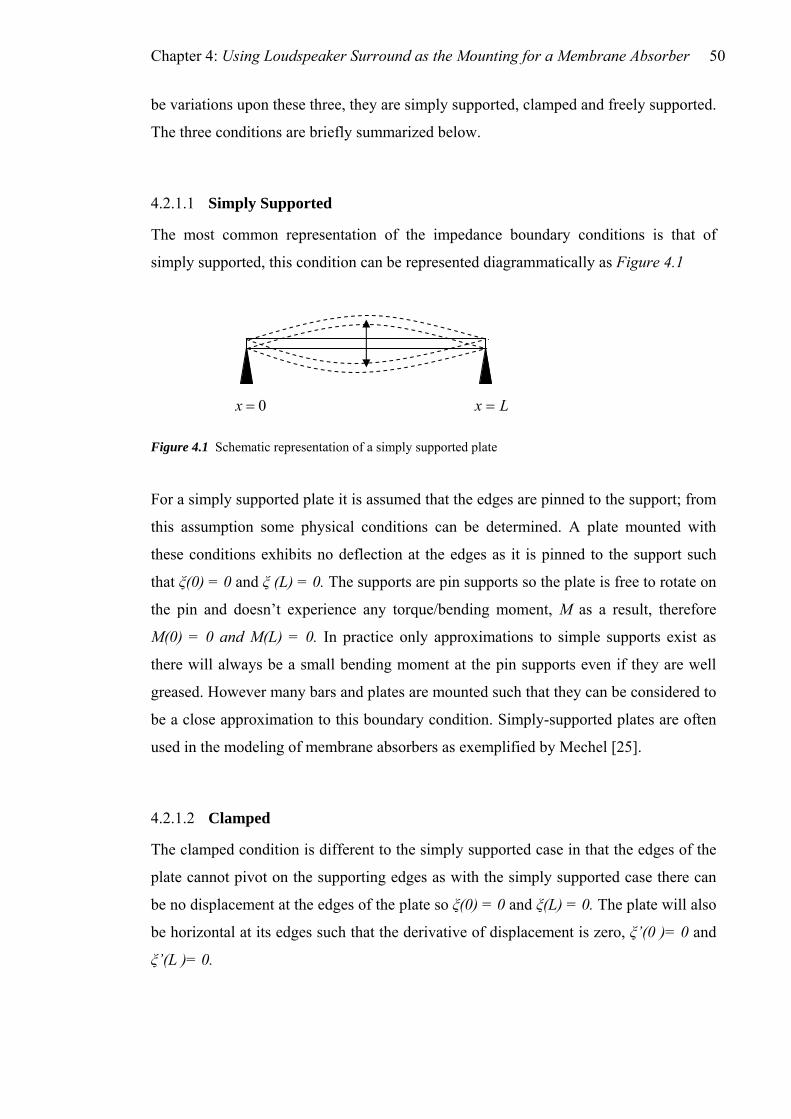
Chapter 4: Using Loudspeaker Surround as the Mounting for a Membrane Absorber 50
be variations upon these three, they are simply supported, clamped and freely supported.
The three conditions are briefly summarized below.
4.2.1.1 Simply Supported
The most common representation of the impedance boundary conditions is that of
mply supported, this condition can be represented diagrammatically as Figure 4.1
Clamped
he clamped condition is different to the simply supported case in that the edges of the
plate cannot pivot on the supporting edges as with the simply supported case there can
ξ(0) = 0 and ξ(L) = 0. The plate will also
si
Figure 4.1 Schematic representation of a simply supported plate
For a simply supported plate it is assumed that the edges are pinned to the support; from
this assumption some physical conditions can be determined. A plate mounted with
these conditions exhibits no deflection at the edges as it is pinned to the support such
that ξ(0) = 0 and ξ (L) = 0. The supports are pin supports so the plate is free to rotate on
the pin and doesn’t experience any torque/bending moment, M as a result, therefore
M(0) = 0 and M(L) = 0. In practice only approximations to simple supports exist as
there will always be a small bending moment at the pin supports even if they are well
greased. However many bars and plates are mounted such that they can be considered to
be a close approximation to this boundary condition. Simply-supported plates are often
used in the modeling of membrane absorbers as exemplified by Mechel [25].
4.2.1.2
0=x Lx =
T
be no displacement at the edges of the plate so
be horizontal at its edges such that the derivative of displacement is zero, ξ’(0 )= 0 and
ξ’(L )= 0.

Chapter 4: Using Loudspeaker Surround as the Mounting for a Membrane Absorber 51
The clamped condition can be drawn diagrammatically as:
An applied force causes plate to bend at the boundary
0=x Lx = Figure 4.2 Schematic representation of a clamped plate
A clamped plate is often a good assumption to make when modeling membrane
absorbers as panels are often screwed or glued providing a strong fixing at the boundary
and allowing no pivotal movement.
igure 4.3 Schematic representation of a freely supported plate
he freely supported case, the difference is that for the pistonic case there is a
storing force introduced by a spring of stiffness, k. The spring provides a restoring
force of kξ to the plate, there will also be a damping associated with the spring applying
4.2.1.3 Freely Supported
This case is probably the theoretically the simplest case although is difficult to create in
practice. A freely supported plate has no bending moment at the edges such that, M(0) =
0 and M(L) =0 and there is no force acting on the edges of the plate as there are no
supports.
Diagrammatically a freely supported plate can be drawn as:
Lx = 0=x
F
4.2.2 The Pistonic Case
Aside from these three common boundary conditions a pistonic case can also be
defined. The pistonic case allows the movement of the plate only in one dimension
similar to t
re

Chapter 4: Using Loudspeaker Surround as the Mounting for a Membrane Absorber 52
a force Ru to the system. Finally the mass of the plate will also apply a force ofdtduM .
This means that the plate w governed by these parameters such
that its resonant frequency
ill oscillate with motion
can be given by:
kπ2 m
f 1=
(4.1)
c compliance of the enclosed volume of air.
embrane absorber is a very
seful tool because it enables the plate to be modeled as a lumped mass; that is, there is
no need to determine the material constants such as its modulus of elasticity or Poisson
ratio. All that is needed is the mass and area of the plate and the stiffness/compliance of
any restoring springs. Damping terms are harder to quantify but techniques borrowed
from modeling porous media and also from loudspeaker design can help.
associated with the design and application of membrane absorbers
rately predict the system’s resonant frequency as seen in
eason for this is that it is very difficult to quantify exactly
system’s resonant behaviour will result. Commercially this could lead to an absorber
The pistonic case can be represented diagrammatically as:
mk
Figure 4.4 Schematic presentation of pistonic mounting
In practice if the plate is mounted on a cabinet, the spring stiffness will also depend on
the acousti
Using the pistonic condition for modeling the plate of the m
u
A perennial problem
is that it is difficult to accu
section 2.4.2.1 The main r
what the mounting conditions of the plate are; the interaction between the membrane
and the cavity is also a difficulty even with advanced numerical techniques such as
finite element modeling. With the mounting condition of the plate approximating a
pistonic condition, modeling will be easier and more accurate predictions of the

Chapter 4: Using Loudspeaker Surround as the Mounting for a Membrane Absorber 53
design that would resonate at lower frequency with greater efficiency and be designed
more easily such that it would resonate at the designated frequency when built.
4.3 Measurements
The theory of using a loudspeaker surround a
s the mounting for a membrane absorber
as tested using an accelerometer and the impedance tube. Results showed that the
resonant frequency uction of
the surround as a consequence of the additional moving mass.
wo scenarios of mounting were tested for the absorber system, firstly with the plate
approximating a clamped condition and secondly with the plate approximating a
pistonic case. Initial tests were carried out on the two conditions, testing the
fundamental resonant frequency of each case using an accelerometer stuck to the centre
und was obtained by request from KEF
oudspeakers and the vinyl rubber plate fixed to it to test the pistonic case. The
rings were cut from a sheet of
mm plywood, these rings were used to clamp the sample being tested, the rings and
w
of the system was decreased dramatically with the introd
4.3.1 Initial Measurements Using an Accelerometer
T
of the plate in question. A 12” loudspeaker surro
L
surround’s mechanical properties were such that it had a large stiffness and a reasonably
heavy damping for a surround of its size. Two mounting
3
sample together then being screwed to a loudspeaker cabinet as per Figure 4.5.

Chapter 4: Using Loudspeaker Surround as the Mounting for a Membrane Absorber 54
Figure 4.5 Photos of membrane mounting
The rings were used so the mounting conditions were the same each time hence it was
just the effect of the surround being tested. Using the rings meant that the area being
tested was the same for both conditions i.e. the area of the surround with the plate and
the plate alone was the same. The surround had a mass/unit area of the 2.381 kgm-2 and
the vinyl membrane of 2.81 kgm-2. The membrane system was ex a
(a) Wooden Mounting Rings (b) Floor tile mounted on surround
(c) Clamped condition (d) Pistonic condition
cited with 12 inch
udspeaker from a distance of 1 metre, using a swept sine signal from a winMLS
controlled computer, an impulse response was generated as measured with the
accelerometer, the windowed Fourier Transform was then taken to obtain a frequency
spectrum from which the results were analysed.
lo

Chapter 4: Using Loudspeaker Surround as the Mounting for a Membrane Absorber 55
WinMLS
Accelerometer
Loudspeaker driver
Power Amp
Accelerometer pre-amp
Sealed cabinet
1m
Figure 4.6 Experimental setup for the accelerometer tests
Both the driver and the absorber were placed on the ground with absorbent in between
to reduce the effect of first order reflections. The experimental setup is shown in Figure
4.6.
esults were processed in MATLAB using the script in Appendix E. The accelerometer
R
was a Knowles BU-1771 with a mass of just 0.28g and dimensions 7.9mm by 5.6mm by
4.1mm. As such it was considered that the additional loading of the accelerometer on
the plate was negligible. The following graph shows the frequency responses obtained
from the measurements.

Chapter 4: Using Loudspeaker Surround as the Mounting for a Membrane Absorber 56
40 60 80 100 120 140 160 180 200-120
0
-100
-80
-60
-40
-20
Frequency, Hz
Leve
l, dB
Acceleration Level versus Frequency For Different Mounting Conditions
55.5Hz
With SurroundWithout Surround
94Hz
proximately 38.5 Hz, a shift of some 41% confirming the
theory that the difference in boundary condition does produce a lower resonant
frequency of significant proportion.
4.3.2 Impedance Tube Tests
The impedance tube as described in chapter 3 had two sample holders of differing
depths (10cm and 30cm), initial tests were carried out using the larger of the two sample
holders as this had a similar volume and hence similar compliant load on the plate as the
loudspeaker cabinet used for the initial accelerometer tests. The membrane was
mounted on the sample holder using two rings (see photo in Appendix F) and jacked up
onto the impedance tube to provide a good seal. The rings were like those used
previously with the accelerometer tests as this corresponded to the similar boundary
conditions, the outer diameter of the rings being larger to allow a tight fit in the tube.
Figure 4.7 Results from the accelerometer tests
Figure 4.7 shows clearly the shift in the fundamental resonance frequency of the system
between boundary conditions approximating clamped and pistonic. The decrease in
resonant frequency is ap

Chapter 4: Using Loudspeaker Surround as the Mounting for a Membrane Absorber 57
Tests were carried out using a swept sine signal at all four microphone positions and
then processed using MATLAB. The tests yielded the following results:
40 60 80 100 120 140 160 180 200 220 2400
0.2
0.4
0.6
0.8
1
Absorption Versus Frequency for Different Mounting Conditions Measured in Impedance Tube
With SurroundWithout Surround
Abs
orpt
ion
Coe
ffici
ent
Frequency, Hz
60Hz 81Hz
ped condition, without the surround to the pistonic
ondition, with the surround. This shift in resonant frequency corresponds to a 26%
decrease. This decrease is less than determined from the accelerometer tests; this is due
at acted as the backing volume in each case. The
Figure 4.8 Results from impedance tube tests with and without surround in large sample holder
Figure 4.8 shows that when measured in the impedance tube the fundamental resonant
frequency shifts 21Hz from the clam
c
to the differences in the cabinets th
sample holder for the impedance tube had a volume of 0.0212m3 where as the
loudspeaker cabinet had a volume of 0.0434m3. An increase in volume corresponds to
an increase in compliance which leads to a lower resonant frequency; this explains why
the case with the surround in the impedance tube resonates at a higher frequency than
when tested on the cabinet with the accelerometer. A further difference seen between
the two tests is that with the clamped case, measured in the impedance tube, the
resonant frequency is lower than with the accelerometer tests, this is a consequence of
the difference in mounting conditions as shown diagrammatically in Figure 4.9.

Chapter 4: Using Loudspeaker Surround as the Mounting for a Membrane Absorber 58
The rings used for the impedance tube tests had a wider outer diameter to account for
the diameter of the impedance tube; this provided a larger surface area for reception of
the incident wave. The clamping of the sample in the impedance tube acts primarily on
the mounting rings rather than on the edge of the membrane, this means that the
impedance at the edge of the clamped plate is less than for the accelerometer tests. T e
us there
ill be a greater moving mass, as the plate is effectively larger hence the fundamental
Test plate
Accelerometer mounting
Impedance tube mounting
Figure 4.9 Illustration of differing clamping conditions in accelerometer and impedance tube tests
a a
Clamping acts on edge of plate Clamping acts on
edge of mounting rings
Less rigid termination at edge of plate
a2
Wall of impedance tube
Mounting rings
Mounting rings
Fixing screws
h
mounting rings will therefore also support bending waves (See Figure 4.10), th
frequency
w
is lower in the impedance tube than with the accelerometer.

Chapter 4: Using Loudspeaker Surround as the Mounting for a Membrane Absorber 59
Vibration of plate and mounting rings
Vibration of plate on surround
Porous absorbent
Impedance tube
Figure 4.10 Samples mounted in impedance tube, demonstrating how mounting rings can support modal
behaviour
When the mass of the clamped plate is larger, the change in moving mass will be less
when mounted pistonically, thus the frequency shift between the two will not be as
great. It can therefore be deduced that the effect of adding the surround is less
pronounced at lower frequencies. This is demonstrated more clearly in t
Rigid backing
he tests done on
a hardboard plate below.
If the plate is mounted on a cabinet of smaller volume the difference that the additional
moving mass makes will be less. This can be seen when the plate was tested in the
smaller of the two sample holders:

Chapter 4: Using Loudspeaker Surround as the Mounting for a Membrane Absorber 60
50 100 150 200 2500
0.1
0.2
0.3
0.4
0.5
0.6
0.7
0.8
0.9
1
Frequency, Hz
Abs
orpt
ion
Coe
ffici
ent
Absorption of Membrane With and Without Surround in Small Sample Holder
With SurroundWithout Surround
105 Hz 96 Hz
Figure 4.11 Results from impedance tube tests with and without surround in small sample holder
.11 shows a frequency shift of the fundamental resonant peak of just 9Hz
orresponding to shift of just 9%. Secondary peaks have been circled on the graph;
requency. The second resonant mode of the system as a whole
an be seen at 230Hz for the clamped condition.
tested, results found that the double resonance
disappeared confirming that it was a consequence of the material properties rather than
the test set up. Results of the hardboard tests in both the large and small sample holder
are given in Figure 4.12.
Figure 4
c
these correspond to a double resonance in the material which is made up from two
distinct layers. The peaks appear at higher amplitudes than with the larger sample holder
case because they are closer in frequency to the fundamental mode of the membrane
thus there is a modal superposition such that the combination of the two peaks results in
greater amplitude at that f
c
The tests were repeated in the impedance tube using a different material, this time it was
3mm thick hardboard that was
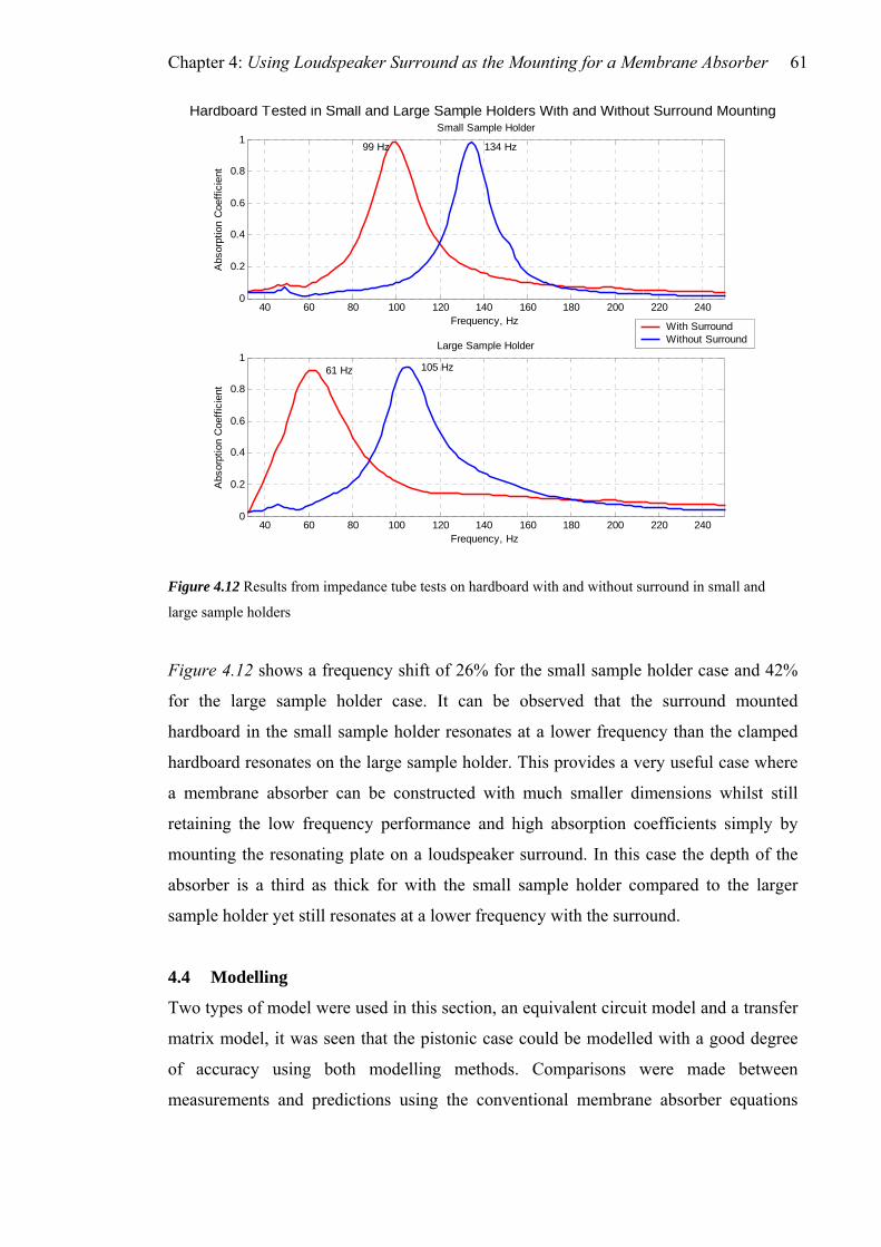
Chapter 4: Using Loudspeaker Surround as the Mounting for a Membrane Absorber 61
40 60 80 100 120 140 160 180 200 220 2400
0.2
0.4
0.6
0.8
1Large Sample Holder
Abs
orpt
ion
Coe
ffici
ent
Frequency, Hz
40 60 80 100 120 140 160 180 200 220 2400
0.2
0.4
0.6
0.8
1Small Sample Holder
Frequency, Hz
Abs
orpt
ion
Coe
ffici
ent
With SurroundWithout Surround
Hardboard Tested in Small and Large Sample Holders With and Without Surround Mounting
134 Hz 99 Hz
105 Hz 61 Hz
uch smaller dimensions whilst still
ply by
odel were used in this section, an equivalent circuit model and a transfer
atrix model, it was seen that the pistonic case could be modelled with a good degree
of accuracy using both modelling methods. Comparisons were made between
measurements and predictions using the conventional membrane absorber equations
Figure 4.12 Results from impedance tube tests on hardboard with and without surround in small and
large sample holders
Figure 4.12 shows a frequency shift of 26% for the small sample holder case and 42%
for the large sample holder case. It can be observed that the surround mounted
hardboard in the small sample holder resonates at a lower frequency than the clamped
hardboard resonates on the large sample holder. This provides a very useful case where
a membrane absorber can be constructed with m
retaining the low frequency performance and high absorption coefficients sim
mounting the resonating plate on a loudspeaker surround. In this case the depth of the
absorber is a third as thick for with the small sample holder compared to the larger
sample holder yet still resonates at a lower frequency with the surround.
4.4 Modelling
Two types of m
m

Chapter 4: Using Loudspeaker Surround as the Mounting for a Membrane Absorber 62
illustrating that greater accuracy in prediction can be made when considering the
pistonic rather than the clamped case.
4.4.1 Equivalent Circuit Model
The theory for equivalent circuit modeling is found in section 5.3.1.1. The equivalent
circuit for the absorber system described in this section is of a simpler form than that
described in chapters five and six. It consists of only a mechanical and acoustical
section such that the analogue circuit that describes its motion can be given as:
is the resistive losses in the cabinet, M is the
determined by
eighing the plate, ZAF is equal to ρ0c/SD if the absorber is within the impedance tube or
ion 5.19 if in free field. RAD, can be estimated from a loudspeaker
inp2
ADM ADR ADC ABR ABC
AFZ
Figure 4.13 Equivalent circuit for a membrane absorber
CAB is the compliance of the cabinet, R
AB AD
mass of the plate, RAD is the resistive losses due to the mounting of the plate, CAD is the
compliance of the surround and ZAF is the radiation impedance which is dependent on
whether the absorber is in a tube or in free field conditions (see section 5.3.3). All of the
above quantities are in acoustic units.
4.4.1.1 Finding Parameters
Before the above circuit can be modeled and the surface impedance found it is
necessary to determine some of the constants in the system. MAD is easily
w
is given by equat
model, RAB is determined from the Delany and Bazley model of porous media [10] and
CAB = V/ρ0c2. CAD is the hardest to determine and requires a simple experimental
procedure as described in section 4.4.1.1.1.

Chapter 4: Using Loudspeaker Surround as the Mounting for a Membrane Absorber 63
4.4.1.1.1 Determining CAD
The compliance of the surround is given by its displacement when given a force F.
ssuming Hook’s law the force applied to the spring (surround) should be proportional
stiffness of the surround and from that to
determine its compliance the following test set up was used:
Figure 4.14 Experimental setup for measuring compliance of surround
he surround, the
isplacement was then measured to a hundredth of a millimeter by the dial gauge which
ia
nd hence the compliance could be found.
A
to its displacement. In order to find the
Added mass
Dial Gauge Clamped Support
Surround
Incremental changes in the mass applied to the plate displaced t
d
was held with a clamp stand to keep it from moving. Masses were positioned carefully
such that equal force was applied to the entire surround. The plate used was rigid
hardboard so it was only the compl nce of the surround being measured rather than that
of the plate itself. A graph as shown in Figure 4.15 was plotted of force applied versus
displacement from which the stiffness a

Chapter 4: Using Loudspeaker Surround as the Mounting for a Membrane Absorber 64
0 0.5 1 1.5 2 2.5 3 3.5 4 4.5
x 10-4
0
0.2
0.4
0.6
0.8
1
1.2
1.4
1.6
1.8
2
Deflection of Surround, m
Forc
e A
pplie
d, N
round (Force Applied versus Deflection of Surround)Finding Compliance of Sur
Measured Data PointsLeast Squarres Best Fit Line
nd
(4.2)
easurement is given as 1.26% which is significantly less
than the 10% error often quoted as the error in the compliance as measured by MLSSA
in the added mass method of small-signal parameters [26] (see section 5.3.3).
Having determined the parameters governing the pistonic case the equivalent circuit can
be solved easily. The equivalent circuit for the clamped case is the same but deriving the
compliance and mass are difficult and as such an equivalent piston of the plate can be
considered.
4.4.1.1.2 Finding the Equivalent Piston of a Clamped Plate
Figure 4.15 Results from experiment to determine compliance of surrou
A regression analysis was performed on the measured data and the corresponding best
fit line plotted. The gradient of the best fit line gives the stiffness of the surround, the
reciprocal of which gives the compliance. The compliance of the surround was found to
be:
-1μmN 2.59 205.49 ±=ABC
The percentage error in this m

Chapter 4: Using Loudspeaker Surround as the Mounting for a Membrane Absorber 65
Assuming a clamped plate with a Poisson ratio, μ thickness, h and Young’s modulus, E
it is possible to determine the equivalent mass and compliance of the plate as an
equivalent piston. Rossi [27] presents such theory. By calculating the kinetic and
potential energy of the plate as it is deflected by the standard parabolic deflection and
integrating over its area it is possible to find an equivalent mass and compliance as if
the plate were a pistonic resonator. Rossi gives the equivalent mass as one fifth of the
mass of the clamped plate and the compliance as:
( )3
221180Eh
aCMEμ−
=
(4.3)
These values can be put into the equivalent circuit model such that the pistonic case can
be compared with the clamped case.
.4.1.2 Results
lerometer tests so as to eliminate the uncertainties in the boundary conditions of the
ounting rings:
4
The equivalent circuit was implemented in MATLAB using the code in Appendix G
plotting the equivalent circuit for the pistonic case and the clamped condition yields
Figure 4.16. The scenario that was modeled was the same as with the initial
acce
m

Chapter 4: Using Loudspeaker Surround as the Mounting for a Membrane Absorber 66
0 50 100 150 200 250 300 350 4000
0.2
0.4
0.6
0.8
1
Equivalent Circuit Model of Membrane Absorber With and Without Surround Mounting
on C
oeffi
cien
t
With SurroundWithout Surround55 Hz 95 Hz
Frequency, Hz
Abs
orpt
i
Figure 4.16 Absorption curve from equivalent circuit model of membrane with and without surround
ll absorption of the system as it shows large inaccuracies in prediction
f the absorption bandwidth. These inaccuracies result because a plate is a complex
element, the equivalent piston model calculated an equivalent compliance and mass
assuming the plate was at its fundamental resonance so outside of that range it is
unsurprising that the model is inaccurate.
4.4.2 Transfer Matrix Model
A transfer matrix model was formulated using the principles described in section
2.4.2.1.1. The MATLAB script can be found in Appendix H. Results were compared to
values as measured in the impedance tube for both the vinyl rubber case and the
hardboard case.
The model accurately predicts the resonant frequency of both cases suggesting that the
change in frequency is almost entirely due to the increase in moving mass of the
s a result of the surround mounting. The model demonstrates that the
equivalent piston for the vibrating plate can be used to predict the resonant frequency
but not the overa
membrane a
o
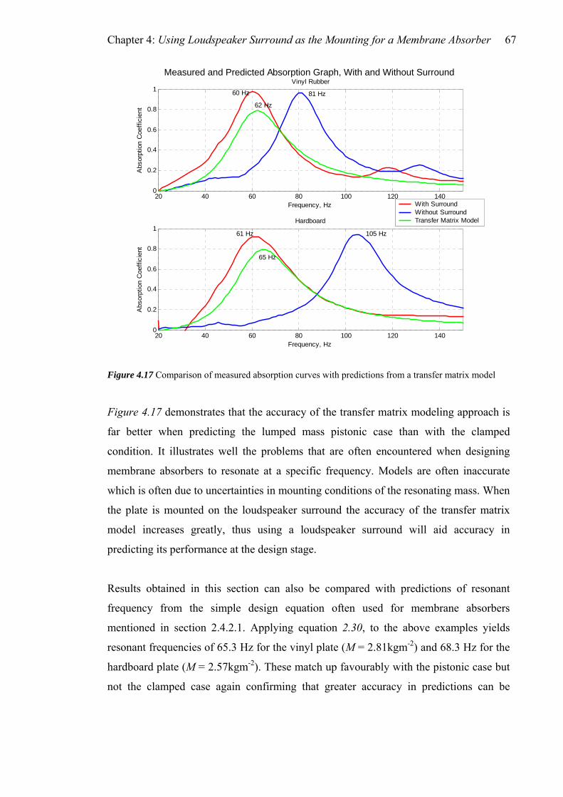
Chapter 4: Using Loudspeaker Surround as the Mounting for a Membrane Absorber 67
20 40 60 80 100 120 1400
0.2
0.4
0.6
0.8
1Vinyl Rubber
Frequency, Hz
Abs
orpt
ion
Coe
ffici
ent
With SurroundWithout SurroundTransfer Matrix Model
20 40 60 80 100 120 140
1
0.8
0.6
0.4
0.2
0
Hardboard
Abs
orpt
ion
Coe
ffici
ent
Frequency, Hz
Measured and Predicted Absorption Graph, With and Without Surround
60 Hz 81 Hz
62 Hz
105 Hz 61 Hz
65 Hz
loudspeaker surround will aid accuracy in
redicting its performance at the design stage.
can also be compared with predictions of resonant
orbers
for the
M = 2.57kgm-2). These match up favourably with the pistonic case but
not the clamped case again confirming that greater accuracy in predictions can be
Figure 4.17 Comparison of measured absorption curves with predictions from a transfer matrix model
Figure 4.17 demonstrates that the accuracy of the transfer matrix modeling approach is
far better when predicting the lumped mass pistonic case than with the clamped
condition. It illustrates well the problems that are often encountered when designing
membrane absorbers to resonate at a specific frequency. Models are often inaccurate
which is often due to uncertainties in mounting conditions of the resonating mass. When
the plate is mounted on the loudspeaker surround the accuracy of the transfer matrix
model increases greatly, thus using a
p
Results obtained in this section
frequency from the simple design equation often used for membrane abs
mentioned in section 2.4.2.1. Applying equation 2.30, to the above examples yields
resonant frequencies of 65.3 Hz for the vinyl plate (M = 2.81kgm-2) and 68.3 Hz
hardboard plate (

Chapter 4: Using Loudspeaker Surround as the Mounting for a Membrane Absorber 68
achieved when using a pistonic lumped mass rather than a clamped plate as the mass of
a membrane absorber.
4.5 Conclusion
Two mounting conditions of a membrane absorber have been considered, firstly a
clamped case as is typical of most membrane absorbers and secondly a pistonic
mounting condition with the use of a loudspeaker surround. Tests were initially
performed with an accelerometer on the membrane and results showed a significant
decrease in resonant frequency with the membrane mounted on the surround. Further
tests were carried out with the low frequency impedance tube confirming the findings of
the accelerometer tests. It was shown the decrease in resonant frequency was a result of
the increased moving mass introduced by the surround. These effects were more
pronounced when the compliance of the cavity was greater i.e. the backing volume was
larger and when the initial mass was smaller. Tests demonstrated that frequency shifts
in excess of 40% could be obtained by using a surround mounting in preference of a
a
udspeaker surround on the small sample holder (a third of the volume of the larger
of the clamped plate and the compliance
s a function of the material constants, Poisson ratio and Young’s modulus. The
Standard membrane absorber design equations were also shown to produce more
accurate results for the surround mounted condition.
standard clamped condition. It was also shown that a membrane absorber utilising
one) could
lo
produce a lower resonant frequency than the clamped case using the larger
sample holder. This illustrates a significant improvement in the low frequency
performance of membrane type absorbers.
An equivalent circuit model was presented, demonstrating that the difference in
resonant frequency was indeed a result of the increased moving mass. The model
included equivalent mass and stiffness terms of a clamped plate moving as a piston. The
pistonic mass modelled as one fifth of the mass
a
equivalent circuit model predicted accurately the resonant frequency of both clamped
and pistonic cases, but approximating the clamped plate as an equivalent piston lead to
inaccuracies in predicting the broadband absorption characteristics. A transfer matrix
model was also demonstrated showing that the pistonic case could be modelled to a
much better degree of accuracy than the clamped case thereby aiding the design of
membrane absorbers such that a trial and error approach need not be employed. The

Chapter 5: Using a Loudspeaker as a Resonant Absorber 69
5. USING A LOUDSPEAKER AS A
RESONANT ABSORBER
5.1 Introduction
Having outlined the theory and practice of using a loudspeaker surround as the
mounting for a membrane absorber, a logical progression is to attempt to use the entire
loudspeaker system as part of the resonant absorber. This is a topic that has been
considered previously by Sato and Koyasu [28] although in this case it was the
incidental absorption of low frequencies by obsolete loudspeakers within a room, seen
as a problem rather than a solution that was considered.
This section aims at the purposeful use of loudspeakers as absorber systems. A
loudspeaker within an enclosure very closely approximates a membrane absorber, the

Chapter 5: Using a Loudspeaker as a Resonant Absorber 70
di
sp
aphragm as the resonating mass, the compliance of the enclosure as the restoring
ring and porous material within the enclosure providing additional damping. Using a
udspeaker as an absorber has several advantages. Firstly loudspeakers already
oscillate naturally, as designed, in a pistonic manner allowing the increased low
equency performance and accurate predictions outlined in the previous chapter.
ily available for rudimentary acoustic
eatment. Thirdly, and possibly the greatest advantage of using a loudspeaker, is that it
an electromagnetic system, hence the electrical and magnetic coefficients of the
stem will affect its mechanical behaviour according to Faraday’s laws of
ectromagnetism. This has the consequence of allowing the system to be tuned to a
ecific resonant frequency, within certain bounds, simply by the addition of resistive
and reactive electrical components across the terminals of the driver, an idea previously
r six. For now
al electronic components is
lumped element prediction model of a loudspeaker used as an absorber is first
esented in this chapter followed by results from impedance tube measurements that
nfirm the predicted data, demonstrating a loudspeaker-absorber that achieves high
sorption coefficients within its resonance region.
2 Basic Premise from Loudspeaker Theory
Most loudspeakers work by supplying a varying current i to a coil of wire length l
d of flux density B which consequently induces a force F = Bil on
rber the system will have a
haracteristic resonant frequency governed by its mechanical and acoustical properties,
lo
fr
Secondly, loudspeakers are cheap and read
tr
is
sy
el
sp
applied to the field of loudspeaker design [29]; this is the focus of chapte
the simple case of a passive loudspeaker with no addition
considered as an absorber system.
A
pr
co
ab
5.
within a magnetic fiel
the coil. If some kind of diaphragm is attached to this coil, air is driven into motion
causing small localised pressure changes thus producing an audible output. Using a
loudspeaker as an absorber uses this system in reverse, similar to a moving coil
microphone. Alternating acoustic pressures in ent to the diaphragm force it into
oscillatory motion thus moving the coil in the magnetic field inducing a voltage in the
connected circuitry. As with a typical membrane abso
cid
c
such as the volume of the enclosure, stiffness of springs and the mass per unit area of
Chapter 5: Using a Loudspeaker as a Resonant Absorber 71
the membrane. Its resonant characteristics will however also be dependent on its
electrical and magnetic coefficients giving the loudspeaker-absorber an extra dimension.
To predict the behaviour of this absorber system a standard lumped parameter technique
for loudspeaker analysis can be used. In the next section such a model is presented and
used to analyse the behaviour of the absorber.
5.3 Lumped Parameter Modelling
Acoustical systems can contain up to three spatial dimensions the components of which
all can change temporally. This leads to very complicated solutions obtainable by the
three dimensional wave equation. In the case of the loudspeaker, there is the added
complication of the coupling between the m chanical and electrical systems. Solutions
using techniques such as Finite Element Analysis can be time consuming and difficult,
consequently it is highly desirab
e
le to simplify problems such that they can be
anipulated and solved more easily. The theory of lumped parameter or lumped
ed to be much larger than one
dimension of the system of interest, that dimension need not be considered in
be constant across it. The problem
m
element modelling enables such simplification [30].
5.3.1 Theory
If the acoustic wavelength in a fluid, such as air, is assum
calculations as pressure and velocity are assumed to
therefore is reduced in complexity by elimination of that variable. The application of
this assumption to the acoustics of ducts means that if the diameter of a duct is small
enough with respect to wavelength, plane wave propagation can be assumed down the
duct, this gives rise to the high frequency limit imposed on impedance tubes. Above a
given frequency the acoustic wavelength in air becomes comparable with the
dimensions of the tube and hence propagation can no longer be considered only in the
direction of the tube’s length but also across its width so the plane wave simplification
can not be accurately applied; a more complex propagation model would need to be
considered not making a plane wave assumption.

Chapter 5: Using a Loudspeaker as a Resonant Absorber 72
If this low frequency assumption is taken further, and the wavelength becomes much
larger than all of the dimensions of the device, although varying temporally, each
acoustic variable can be considered constant in the all three directions of the spatial
to that of
nly a single degree of freedom variant only with time. When these conditions are
assumed the components of the system can be considered as a lumped elements or
ering technique and is used extensively in
ut many spheres of science and
ngineering. Drawing a schematic diagram means that the differential equations
en system can be easily determined and solved on inspection. This is
logies between electrical, mechanical
nd acoustical domains such that the equivalent circuits retain their integrity. The
domain, i.e. pressure and velocity are constant across all of its dimensions at a given
moment in time. If these conditions are applied, the equation of motion is greatly
simplified, such that any spatial dependency is removed, reducing the problem
o
lumped parameters. This is a common engine
loudspeaker design and modelling [31, 32].
A major advantage of using a lumped element method is that it is very easy to draw a
schematic representation of a system utilising analogies between mechanical, acoustical
and electrical components; this is common practice for engineers and allows each
section to be represented as an electrical, mechanical or acoustical diagram. Electrical
circuits are commonly chosen as the schematic representation because electrical circuit
theory is widely known and understood thro houg
e
governing a giv
relatively simple if the spatial variables are removed however if the spatial dimensions
are re-introduced for smaller wavelengths or larger devices the differential equations
become very complicated and it becomes profitable to revert to elementary acoustics
and the solution of the wave equation again. As such there is a high frequency limit
imposed on the use of lumped parameter models, which states that the highest
frequency should have a wavelength greater than all the dimensions of the system being
modelled [27].
5.3.1.1 Equivalent Circuits
The premise behind the theory of equivalent circuits is to represent a physical situation,
be it mechanical or acoustical, in the form of an electrical circuit. In order to
successfully do this it is necessary to define ana
a

Chapter 5: Using a Loudspeaker as a Resonant Absorber 73
following, briefly describes two commonly used analogies for the purpose of equivalent
circuit analysis, these are the impedance and mobility analogues.
In terms of electrical oscillations (of great importance in the field of electroacoustics)
there are three principle electronic components each one either storing or dissipating
energy:
- Inductors LE, store magnetic energy (flux)
- Capacitors CE, store electrical energy (charge)
- Resistors RE, dissipate energy
If the current is known, an expression for the potential difference across each
component can be formed such that:
dtdiLv E= ,
EC
dtiv ∫=
. , and iRv E=
(5.1)
Assuming a sinusoidal input current, tjeii ω0= the impedance of these components can
be determined as:
LjivZ
Ljeiev tjtj
ω
ωωω
==
= 00
,
CjivZ
Cjeiev
tjtj
ω
ω
ωω
1
00
==
=, R
ivZ ==
(5.2)
Analogous th to ese three electrical components of oscillation are three mechanical
scillatory components:
- Mass M , stores kinetic energy
o
M
- Compliance CM, stores potential energy
- Frictional resistance (damping) RM, dissipates energy
Chapter 5: Using a Loudspeaker as a Resonant Absorber 74
For the mechanical case, velocity u is the flow variable so can be thought of as
analogous to electrical current and force F is the potential variable and can be thought
f as analogous to voltage. In the same way as for the electrical components, if the
ing equations:
o
velocity of each section in the mechanical components is known and assumed to be
sinusoidal, the force across, and the impedance of the components can be determined by
the follow
From Newton’s law of forcedtMMduMF = and MM MjZ ω=
From Hook’s law M
M C
dtuF ∫=
.
MM Cj
Zω
1= and
From classical mechanics uRF MM = and MM RZ =
(5.3)
side from Newton’s law of force which is universally valid, these are only first order
approximations and therefore are more accurate when small displacements are
considered, with larger displacements the system is no longer linear which complicates
matters and lumped parameter analysis is no longer valid.
al and mechanical cases, the components are assumed to be ideal, so
at, an inductor has no capacitance or resistance and conversely a compliance has no
mass et cetera. This is a useful first approximation and extra components can be added
to a model to account for the fact that they are not in fact ideal, Rossi [27] provides a
more extensive analysis this topic looking at the equivalent mass of an ideal compliance
et cetera. In most situations the elements in the circuit can be considered as ‘lumped’
such that no mechanical or acoustical component exhibits any wave motion withi
s with mechanical values there are three acoustical quantities that pertain to the
at:
- Acoustic compliance CA, stores potential energy
- viscous damping RA, dissipates energy
A
In both the electric
th
n the
element.
A
oscillatory electrical components such th
- Acoustic mass or inertance MA, stores kinetic energy

Chapter 5: Using a Loudspeaker as a Resonant Absorber 75
In the acoustic case, volume velocity U is the flow variable (analogous to current) and
pressure p is the potential variable (analogous to voltage). Therefore if the volume
velocity through a component is known then it is possible to calculate the pressure by
across the components given a sinusoidally oscillating volume velocity by:
dtdUMp A= therefore AA MjZ ω=
AC
dtUp ∫= .
therefore A
A CjZ
ω1
=
therefore URp A= URZ AA =
(5.4)
Combining these analogies leads to the impedance analogue which can be surmised by
Table 5.1:
Impedance Analogue
Electrical Mechanical Acoustical
otential e FM p P
Variable
Voltage, Force, Pressure,
Flow variable Current, i Velocity, u Volume velocity, U ( =
u×S)
Dissipative
component
Resistance, RE
EE RZ =
Damping, RM
MM RZ =
Acoustic damping, RA
AA RZ =
Kinetic storage
component
Inductance, LE
LjZ EE ω=
Mass, MM
MjZ MM ω=
Acoustic mass, MA
MjZ AA ω=
Potential
storage
component EE
Capacitance, CE
CjZ ω/1 MM=
Compliance, CM
CjZ ω/1= A AA
Acoustic compliance ,
CjC , Z ω/1 =
Table 5.1 Summary of the impedance analogue
MM
CA
This impedance analogue is very useful and can be used to model many practical
simply a matter of whether to
her analogy also exists which makes use
scenarios. Using Kirchoff’s current and voltage laws it
connect components in parallel or series. Anot

Chapter 5: Using a Loudspeaker as a Resonant Absorber 76
of the reciprocity of electrical components that is to say that an inductor behaves to
current how a capacitor behaves to voltage and vice versa, i.e.:
dtdeCi E= and
dtdiLe E=
(5.5)
This leads to another analogy which is the reciprocal of the impedance analogy and
consequently called the mobility analogue, so that inductors become capacitors and vice
versa and resistances become conductances (a reciprocal resistance). Any components
that were connecte ill consequently need to be connected in parallel and any
in parallel conne ies in ord logy can be
seen as the direct opposite to the impedance analogue and can be surmised in the
be identical. The impedance analogue is more intuitive,
ysis of loudspeakers to use both impedance
and mobility analogues as it ma ewhat easier as will be
ter:
Mobility Analogue
d in series w
cted in ser er to obey Kirchoff’s laws. This ana
following in Table 5.2. Because they are complete opposites of each other, the results
yielded by both analogies will
however it is useful especially in the anal
kes combining the circuits som
seen la
Electrical Mechanical Acoustical
Potential
Variable
Current, i Force, FM Pressure, p
Flow variable Voltage, e Velocity, u Volume velocity, U ( =
u×S)
Dissipative Conductance, 1/RE
EE
Damping, RM
MMcomponent RZ /1=
RZ /1=
Acoustic damping, RA
AA RZ /1=
Kinetic storage
t
Capacitance, L
EEcomponenE
LjZ ω/1=
Mass, M
MM
M
MjZ ω/1=
Acoustic mass, M
AA
A
MjZ ω/1=
Potential
storage EE CjZ
component
Inductance, CE
ω=
Compliance, CM
MM CjZ ω=
Acoustic compliance ,
CA , Z AA Cjω=
M M
CA
Table 5.2 Summary of the mobility analogue
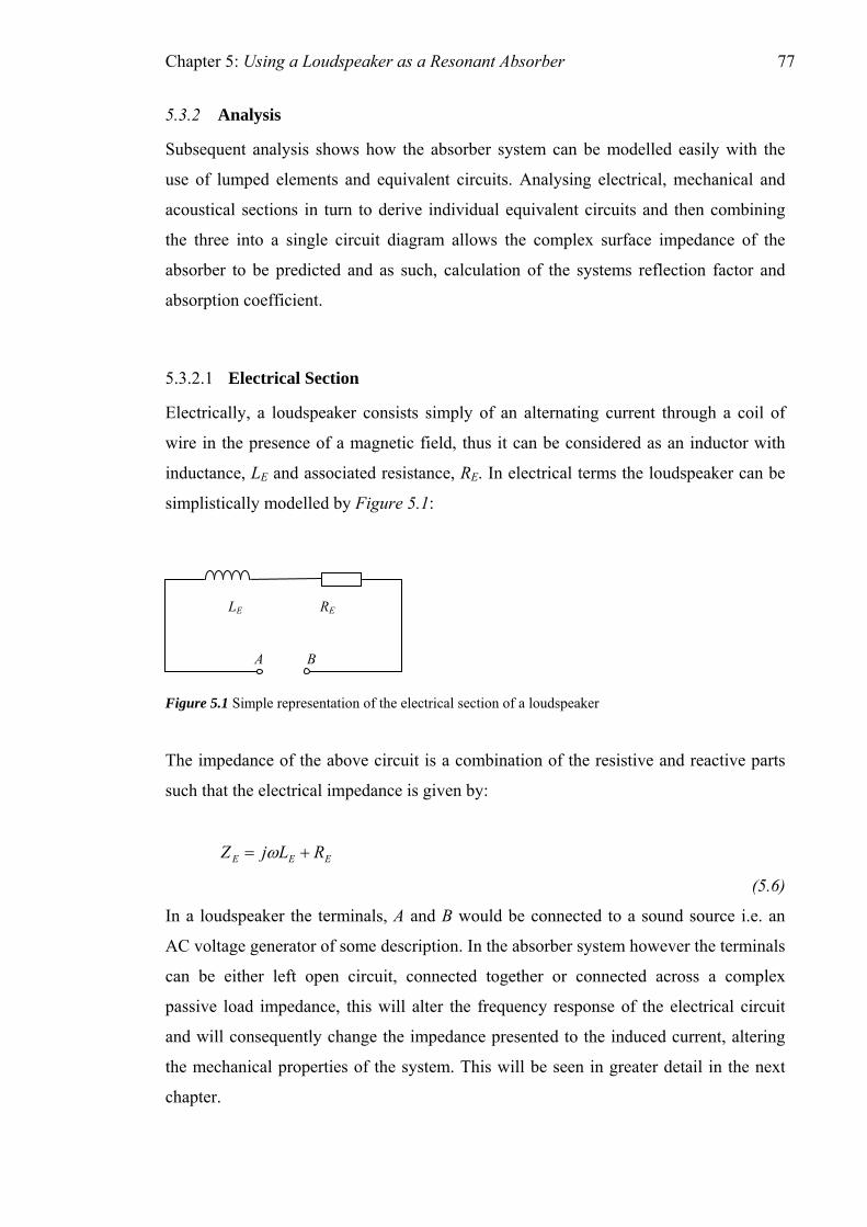
Chapter 5: Using a Loudspeaker as a Resonant Absorber 77
5.3.2 Analysis
Subsequent analysis shows how the absorber system can be modelled easily with the
se of lumped elements and equivalent circuits. Analysing electrical, mechanical and
acoustical section urn to de and then combining
the three into a single circuit diagram allows the complex surface impedance of the
absorber to be predicted and as such, calculation of the systems reflection facto
mple representation of the electrical section of a loudspeaker
it is a com
such that the electrical impedance is given by:
u
s in t rive individual equivalent circuits
r and
absorption coefficient.
5.3.2.1 Electrical Section
Electrically, a loudspeaker consists simply of an alternating current through a coil of
wire in the presence of a magnetic field, thus it can be considered as an inductor with
inductance, L ociated resistance, RE. In electrical terms the loudspeaker can be
simplistically modelled by E and ass
Figure 5.1:
LE RE
A B
Figure 5.1 Si
The impedance of the above circu bination of the resistive and reactive parts
EEE RLjZ += ω
.6)
inals, A nd B would be connected to a sound source i.e. an
generat iption ystem
ither left open circuit, connected together or connected across a comp
pedance, this will alter the frequency response of the electrical circuit
edance presented to the induced current, altering
e mechanical properties of the system. This will be seen in greater detail in the next
chapter.
(5
In a loudspeaker the term a
AC voltage
can be e
passive load im
or of some descr . In the absorber s however the terminals
lex
and will consequently change the imp
th
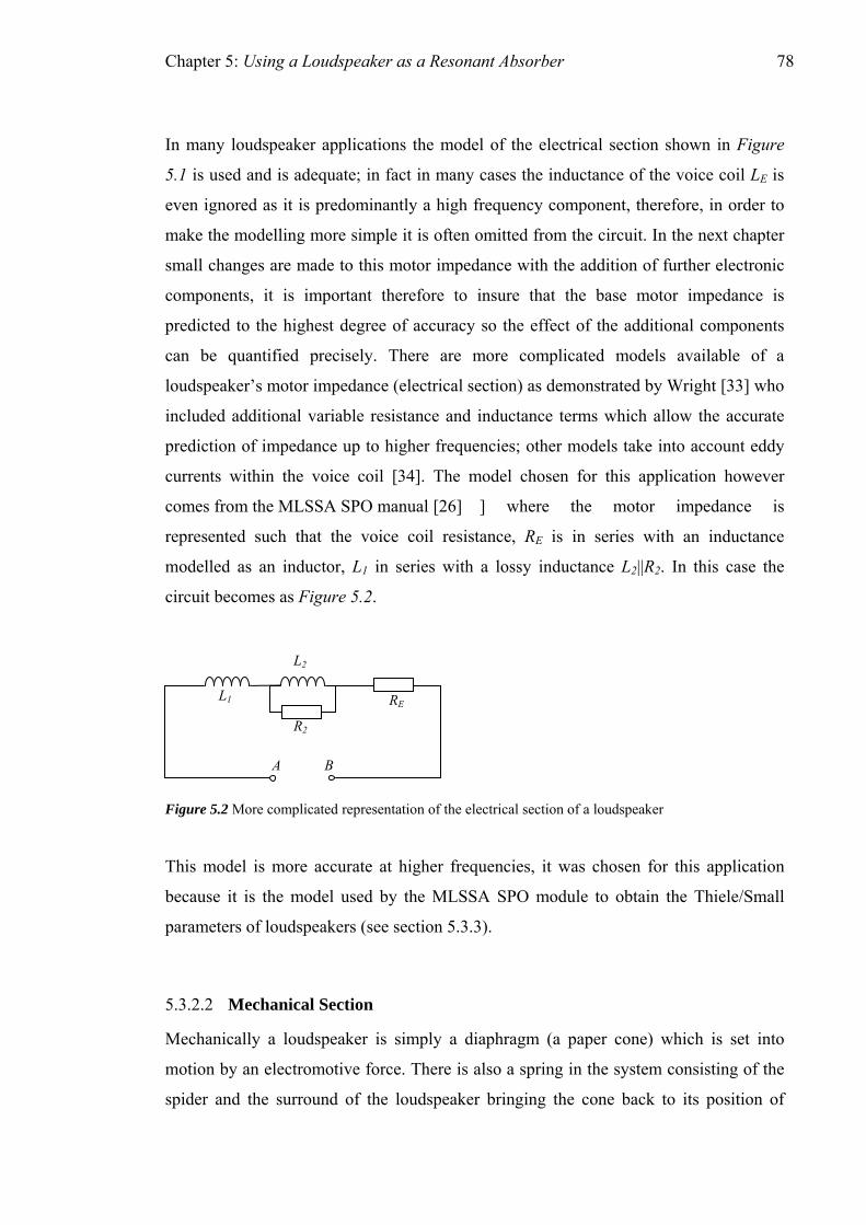
Chapter 5: Using a Loudspeaker as a Resonant Absorber 78
In many loudspeaker applications the model of the electrical section shown in Figure
5.1 is used and is adequate; in fact in many cases the inductance of the voice coil LE is
even ignored as it is predominantly a high frequency component, therefore, in order to
make the modelling more simple it is often omitted from the circuit. In the next chapter
small changes are made to this motor impedance with the addition of further electronic
components, it is important therefore to insure that the base motor impedance is
redicted to the highest degree of accuracy so the effect of the additional components
can be quantified precisely. There are more complicated models available of a
ce (electrical section) as demonstrated by Wright [33] who
] where the motor impedance is
h that the voice coil resistance, RE is in series with an inductance
modelled as an inductor, L1 in series with a lossy inductance L2||R2. In this case the
circuit b es as Figure 5.2.
igure 5.2 More complicated representation of the electrical section of a loudspeaker
This model is more accurate at higher frequencies, it was chosen for this application
because it is the model used by the MLSSA SPO module to obtain the Thiele/S
the surround of the loudspeaker bringing the cone back to its position of
p
loudspeaker’s motor impedan
included additional variable resistance and inductance terms which allow the accurate
prediction of impedance up to higher frequencies; other models take into account eddy
currents within the voice coil [34]. The model chosen for this application however
comes from the MLSSA SP [O manual 26]
represented suc
ecom
L2
F
mall
parameters of loudspeakers (see section 5.3.3).
5.3.2.2 Mechanical Section
Mechanically a loudspeaker is simply a diaphragm (a paper cone) which is set into
motion by an electromotive force. There is also a spring in the system consisting of the
spider and
RE L1
R2
A B

Chapter 5: Using a Loudspeaker as a Resonant Absorber 79
equilibrium each time it is displaced. The spider works at the apex of the cone and the
r
ternating current that is applied across the terminals. The
bsorber system uses the loudspeaker in reverse to induce a current in the voice coil
given oscillation of the diaphragm in sympathy with an acoustic pressure. As with a
standar embrane absorber the cone will generate a particle velocity in the cabinet
which is then absorbed by porous material. The absorber will have a resonant frequency
inherently controlled by the moving mass of the diaphragm and the stiffness of the
spring (both the m ension compliance and the compliance of the air
be altered by
hanging these parameters, however this is awkward as it involves rebuilding the entire
nduced current will be impeded by the
lectrical components L1, L2, R2 ,RE and those connected across terminals A and B as
seen from Figure 5.2 components have a frequency dependence of their own,
ll be larger at some frequencies than at others enabling
surround on the outside of the cone ensuring equal force is applied to all areas
e with no phase lag of the combined restoring force. The diaphragm of a
loudspeaker is conical in a shape to increase its stiffness in the plane normal to the
intended motion; this ensures that it moves backwards and forwards as a piston. That
the diaphragm moves with pistonic oscillation is an important assumption to make as it
eliminates the need to model complex bending waves on the diaphragm that appear at
higher frequencies otherwise known as ‘cone break up’. Attempting to model a
loudspeaker using lumped parameter techniques at higher frequencies will lead to
spurious results as bending waves alter both the moving mass and the compliance of the
diaphragm making it a nonlinear system. For lower frequency radiation however the
pistonic assumption is valid and enables accurate predictions.
A magnetic field is generated by a larg manent magnet which is held in place by a
chassis so as not to put a load on the diaphragm. As a consequence of this magnetic
field, the induced movement of the cone is governed in frequency and magnitude by the
frequency and stren al
of the
con
e pe
gth of the
volume within the cabinet). This enables the resonant frequency to
a
d m
echanical susp
c
absorber using different materials and geometry, and this is obviously rather
impractical. It is possible however to use the electrical section of the absorber to change
the resonance in the mechanical domain. The i
e
. These
thus the electrical impedance wi
the induced current to flow more easily at some frequencies. Mechanically the system
will oscillate with greater amplitude when the impedance to the induced current is at a

Chapter 5: Using a Loudspeaker as a Resonant Absorber 80
minimum and as such the electrical section will have ramifications on the resonance
properties of the entire system.
Considering just the mechanical section of the loudspeaker it can be seen that with the
diaphragm moving pistonically, on the combined compliance it can be represented
simply as a mass on a spring as in Figure 5.3:
MM
MR MM CK /1=
F
Figure 5.3 Mechanical representation of a loudspeaker
The mass MM moves on a spring with stiffness MK and compliance MC , there is also
some inherent damping in the mechanical system MR which comprises of losses within
the mounting and suspension of the diaphragm. The above system can be easily solved
using differential equations, such that the equation of motion becomes:
u = 0
∫++= dtuKRdtduMF MMM .
(5.7)
Assuming sinusoidal oscillation, tjeFF ω0= and tjeuu ω
0=
uCj
uRuMjF
euCj
euReuMjeF
MMM
tj
M
tjM
tjM
tj
ωω
ωω ωωωω
1
10000
++=
++=
(5.8)
Mechanical impedance can be written as uFZM /= therefore the total mechanical
impedance of the above system is:

Chapter 5: Using a Loudspeaker as a Resonant Absorber 81
MMMM Cj
RMjZω
ω 1++=
(5.9)
al impedance with an inductor a resistor
nd a capacitor.
l section of a loudspeaker
mec
es
he mechanical section of a loudspeaker
The impedance of this circuit can be determined as follows:
This is the expected result which can also be obtained by modelling the scenario with
the impedance analogue leading to the equivalent circuit shown in Figure 5.4. This
impedance is in the same format a rics an elect
Figure 5.4 Impedance analogue circuit of the mechanica
a
u
MM MR
F
MC
The same hanical system can be modelled with the mobility analogue as the
reciprocal of Figure 5.4 such that the circuit becom as Figure 5.5:
uF MR/1 MC MM
Figure 5.5 Mobility analogue circuit of t
1 2
1 1 1 1...
1 1Tot n
M M
Z Z Z Z
jTot M
M RZ j C
ωω
= + +
= + +
(5.10)
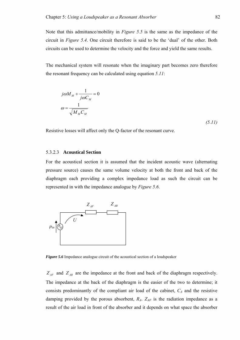
Chapter 5: Using a Loudspeaker as a Resonant Absorber 82
Note that this admittance/mobility e as the impedance of the
circuit in Figure 5.4. One circuit therefore is said to be the ‘dual’ of the other. Both
circuits can be used to determine the velocity and the force and yield the same resul
in Figure 5.5 is the sam
ts.
The mechanical system will resonate when the imaginary part becom refore
the resonant frequency can be calculated using equation
es zero the
5.11:
MM
MM
CM
CjMj
1
01
=
+
ω
ωω
(5.11)
Resistive losses will affect only the Q-factor of the resonant curve.
.3.2.3 Acoustical Section
t and back of the
iaphragm each providing a complex impedance load as such the circuit can be
represented in with the impedance analogue by Figure 5.6.
Figure 5.6 Impedance analogue circuit of the acoustical section of a loudspeaker
and are the impedance a
The impedance at the back of the diaphragm is the easier of the two to determine; it
consists predominantly of the compliant air load of the cabinet, CA and the re
amping provided by the porous absorbent, RA. ZAF is the radiation impedance as a
result of the air load in front of the absorber and it depends on what space the absorber
=
5
For the acoustical section it is assumed that the incident acoustic wave (alternating
pressure source) causes the same volume velocity at b onoth the fr
d
U
ABZAFZ
pin
AFZ ABZ t the front and back of the diaphragm respectively.
sistive
d

Chapter 5: Using a Loudspeaker as a Resonant Absorber 83
‘radiates’ into. When in free space th ce at the front of the diaphragm is a
combination of an acoustic mass term and a resistive air load on the diaphragm given by
the radiation impedance of a baffled piston as in equation
e impedan
5.19. ZAF is less complicated
the absorber radiates in tube with plane wave propagation as is modelled in
y equation 5.20. Greater
etail will be paid to these terms in section 5.3.3.
The mobility analogue can rcuit.
Pressure becomes the flow variable (current), volume velocity the potential variable
(voltage).
.3.2.4 Combining the Sections
Once all of the sections een individually derived it is important to link them
together correctly, this is done using ideal transformers forming an electrical link
between the circuits enabling each section to be written in the same units so the overall
impedance of the system can be determined from a combined circuit of all three
sections.
d to be no losses in
e coils, i.e. they have negligible resistance and inductance such that all power is
cons Th
if
subsequent sections for comparison with impedance tube tests. In this case the mass
term disappears and the radiation impedance can be given b
d
also be used to represent the system as an electrical ci
Figure 5.7 Mobility analogue circuit of the acoustical section of loudspeaker used as a membrane
absorber
5
have b
Ideal transformers are electrical transformers where there is assume
th
erved. erefore for the transformer in Figure 5.8 bvav 12 = and biai = .
21
AZ F
1 ABZ1 inp

Chapter 5: Using a Loudspeaker as a Resonant Absorber 84
Figure 5.8 Idealised transformer
a:b 1Z
1v
In order to calculate the output voltage, v2 when multiplying out the transformer it is
simply a matter of multiplying the input voltage, v1 by the turns ratio (a/b) and to
determine the current in the secondary circuit, the input current is divided by this turns
tio. With this in mind the equivalent impedance, Z2 in Figure 5.9 can also be
determined when multiplying out the transformer to form a single circuit such that:
ra
2
12
2
211 ⎟
⎠⎜⎝⋅=
⎞⎛==
bibiZ 2
21
⎟⎠⎞
⎜⎝⎛⋅=
⎞⎛⎟⎠⎞
⎜⎝⎛
baZZ
avbav
v
(5.12)
Looking from the position of Figure 5.8 and Figure 5.9 are electrically equivalent.
2 ⎟⎠
⎜⎝ a
i
The simplified circuit can then be written as Figure 5.9:
Figure 5.9 Simplified idealised transformer
2v
1i 2i
2v
⎟⎠⎞
⎜⎝⎛
abv
2
12 ⎟⎠⎞
⎜⎝⎛=
abZZ
2i
2v
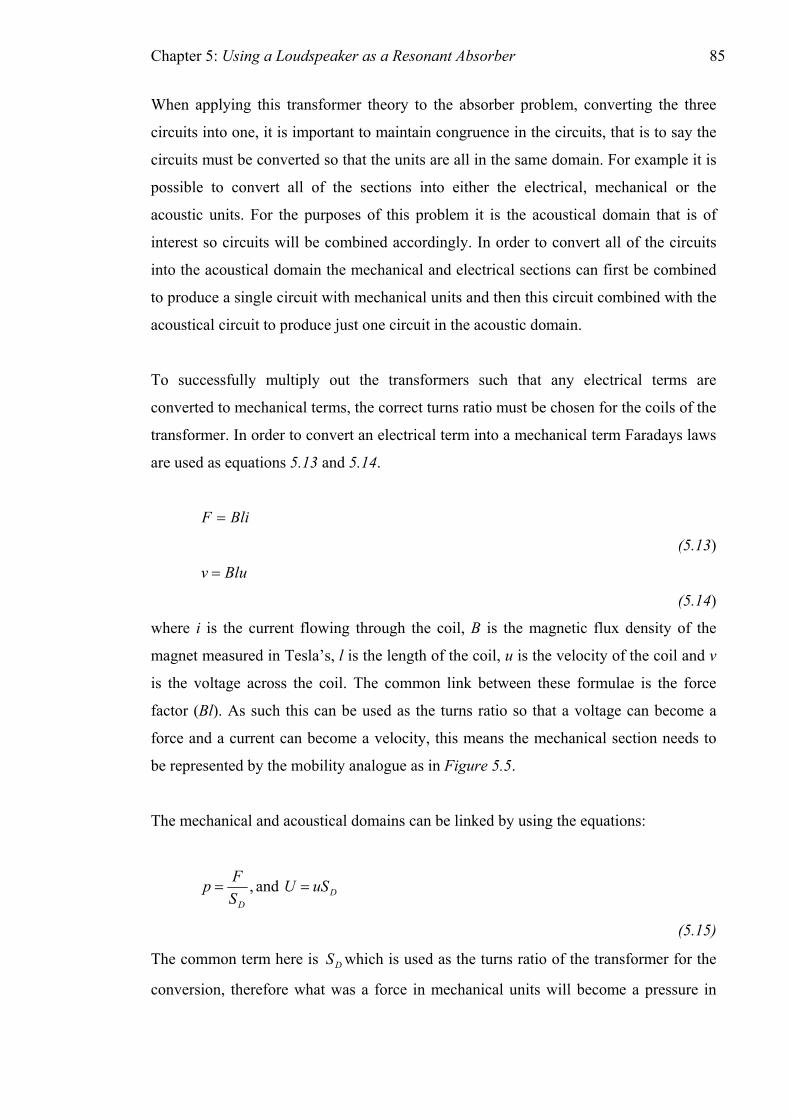
Chapter 5: Using a Loudspeaker as a Resonant Absorber 85
When applying this transformer theory to the absorber problem, converting the three
circuits into one, it is important to maintain congruence in the circuits, that is to say the
circuits must be converted so that the units are all in the same domain. For example it is
possible to convert all of the sections into either the electrical, mechanical or the
acoustic units. For the purposes of this problem it is the acoustical domain that is of
interest so circuits will be combined accordingly. In order to convert all of the circuits
e mechanical and electrical sections can first be combined
produce a single circuit with mechanical units and then this circuit combined with the
aws
re used as equations 5.13 and 5.14.
(5.13)
(5.14)
where i is the current flowing through the coil, B is the magnetic flux density of the
magnet measured in Tesla’s, l is the length of the coil, u is the velocity of the coil and
en these formulae is the force
Bl). As such this can be used as the turns ratio so that a voltage can become a
force and a current can become a velocity, this means the mechanical section needs to
be represented by the mobility analogue as in Figure 5.5.
The mechanical and acoustical domains can be linked by using the equations:
into the acoustical domain th
to
acoustical circuit to produce just one circuit in the acoustic domain.
To successfully multiply out the transformers such that any electrical terms are
converted to mechanical terms, the correct turns ratio must be chosen for the coils of the
transformer. In order to convert an electrical term into a mechanical term Faradays l
a
BliF =
Bluv =
v
is the voltage across the coil. The common e link betw
factor (
,DS D
he turns ra
Fp = and
(5.15)
w e
onversion, therefore what was a force in mechanical units will become a pressure in
uSU =
The common term here is DS h as t tio of the transformer for thich is used
c

Chapter 5: Using a Loudspeaker as a Resonant Absorber 86
the acoustic section and what was a velocity in the mechanical section will now become
a volume velocity. As such the acoustic section needs also to be modelled with the
mobility analogue to prevent an incongruity of values. The three sections linked with
the transformers then becomes as per Figure 5.10:
MDM MDC
Bl:1 1:DS
Acoustical section (Mobility analogue)
Mechanical section (Mobility analogue)
Electrical section (Impedance analogue)
L1 L2
Figure 5.10 Equivalent circuit linking electrical, mechanical and acoustical sections with transformers
The transforme echanical and the electrical sections is removed using the
rules for idealised transformers, dividing impedances by the square of the turn
) thus the circuit becomes:
igure 5.11 Equivalent circuit of membrane absorber with electrical and mechanical sections combined
hat was a current in the electrical section has now become a force in the mechanical
main from equation 5.13 e a velocity from
equation 5.14. Thus the right hand side circuit consists now entirely of components with
mechanical units. The mechano-acoustical transformer is now removed by multi
r linking the m
s ratio
( 1/Bl
F
W
do and what was a voltage has becom
plying
all the impedances by the square of the turns ratio ( )DS/1 . It is the impedance that is
multiplied out rather than the component value hence:
MDM MDC MDR1
1:DS
( )22
BlR
inp AFZ1
( )2BlE R
( )2Bl
( )LE
2Bl 2L
ABZ1
p F
MDR1
inp
AFZ 1
ABZ RE
1R2
p iF

Chapter 5: Using a Loudspeaker as a Resonant Absorber 87
⎟⎟⎠
⎞⎜⎜⎝
⎛=×
2
2 11
D
MD
DMD
SMj
SMj
ωω
so the component value is 2D
MD
SM
(5.16)
e analogue
( )2
2
Bl
Figure 5.12 Equivalent circuit of membrane absorber with electrical, mechanical and acoustical sections
com
bined
e of the components such that it is easier to define
their physical values. The components are renamed as they are now in acoustical units
using the relationship that acoustical impedance can be determined by dividing the
mechanical impedance by a factor of area squared (the operation performed when the
transformer was multiplied out). Taking the dual of the circuit gives:
The circuit in Figure 5.12 can be directly solved to determine the impedance of the
absorber system however it is easier to put the circuit into the impedance analogue by
taking its dual and to rename som
Figure 5.13 Equivalent circuit of membrane absorber in impedanc
inp
AFZ ADC ADM ADR ABZ
( )2SR
( )2 D
2Bl2
2
BlD
2SL
( )2
2
DESRBl
( )22
BlSL DE
SR DE
inp AD
D
MD
MSM
=
2 AD
MD
CSC
=
2
D
p
AFZ1
ABZ1
AD
MD
D
R
S
/1
2
=
( )
R
2Bl
( )
2SL DE
2
2
BlSR DE
( )2
2
BlSL DE

Chapter 5: Using a Loudspeaker as a Resonant Absorber 88
This is the full equivalent circuit in the im
absorber system upon which all subsequent analysis is based.
5.3.3 Defining the Parameters
In order to calculate the impedance of this circuit it is important that the component
values can be determined. These can be obtained using direct theory and also by
measuring the driver’s Thiele/Small signal parameters [31, 32]. The parameters are also
often referred to as small signal parameters because they are physical constants
pertaining to a loudspeaker when operating linearly i.e. when a small signal is applied
rather than a large signal which would cause non-linear behaviour. Measuring the
Thiele/Small parameters of a loudspeaker can be done in several ways [35, 36, 37].
od chosen here was the added mass method. With this method, weights are
dded to the diaphragm such that the additional moving mass decreases the driver’s
pedance analogue for the loudspeaker
The meth
ncy, fS by a
a
resonant freque bout 20%. In the added mass technique MMS is found first
from equation 5.17:
1'
2
−⎟⎟⎠
⎞⎜⎜⎝
⎛=
S
S
ADDEDMS
ff
MM
(5.17)
Where MADDED is the added mass, fS is the drivers’ resonant frequency and sf ′ is the
driver’s resonant frequency with the additional mass. Using this value of MMS the free-
air mechanical compliance of the driver can be obtained from:
( ) MSSMS Mf
C 221
π=
(5.18)
Other parameters can be obtained from performing electrical impedance tests on the
driver. This procedure was done automatically using a maximum length sequence signal
analyser (MLSSA). The parameters that were obtained were:

Chapter 5: Using a Loudspeaker as a Resonant Absorber 89
M g15228.MS = , the mechanical moving mass of the driver with an air load
, the second equivalent resistance of voice coil
he equivalent lossless inductor
a reactive part (mass loading) and a resistive part (damping).
ming pistonic movement of the diaphragm in an infinite baffl
dance of the diaphrag
μmN276385. = CMS , the mechanical compliance of the driver
Ω41512. = R , the DC electrical resistance of the driver voice coil E
Ω0252 . = R
mH90701 . = L , the inductance of t
mH59512 . = L , the inductance of the equivalent lossy inductor
Ω575360. = RES , the mechanical losses of the diaphragm in electrical units
Tm16920.Bl = , the force factor of the driver 2m057680.SD = , the area of the diaphragm
The subscript notation follows the rules for nomenclature as defined in p d I. Ap en ix
The acoustic impedance at the front and back of the diaphragm, given by AFZ and
ABZ respectively, can be expanded in order to determine their values. The impedance at
the front is the radiation impedance; this is a combination of the complex air load on the
driver consisting of
Assu
impe
e, the radiation
m at low frequencies ( 1<ka ) can be written as [15]:
ajckMjRZ AFAFAF 2
02
0
38
2 πρω
πρω +=+=
ith measurements made
the impedance tube the radiation impedance is changed such that it more closely
represents this plane wave case. The radiation impedance of the piston can be
determined by considering e the
ratio of pressure to particle velocity is given as ρ0c such that the acoustic impeda
(5.19)
This would be the radiation impedance if the driver were to be placed in 2π space, i.e.
used within a room. However in order to compare predictions w
in
a plane wave incident to a rigid surface. For such a cas
nce is
given as:
Sc
UpZ A
0ρ==
(5.20)

Chapter 5: Using a Loudspeaker as a Resonant Absorber 90
As pressure is om a plane
surface is equal to 2 can be represented by a
voltage generator of strength
by equation 5.20.
The impedance the compliant load of
the sealed vol losses due to the porous
absorbent in the ten as:
scalar the total pressure when a plane wave is reflected fr
pi therefore in the analogue the plane wave
2pi with a radiation impedance in front of the piston given
at the back of the diaphragm is a combination of
ume of air in the cabinet, ABC and the resistive
cabinet ABR . The compliance of a sealed volume can be writ
20c
VC B AB ρ=
21)
here is the volume of the box. The resistive losses can be determined by an
and
own in
igure 5.14:
(5.
BVw
acoustic model such as the Delany and Bazley empirical model. Although the Delany
Bazley model is inaccurate at very low frequencies it is sufficient for the purposes
of estimating the value of AFR using equations 2.11, 2.12 and 2.13.
From these parameters all of the component values in the circuit can be determined and
the total impedance found. The circuit in Figure 5.13 can be simplified sh as
F
Figure 5.14 Simplified equivalent circuit of membrane absorber
Where:
2D
MSAD S
MM =
(5.22)
inp2
ADM ATR ATCAFZ AEZ
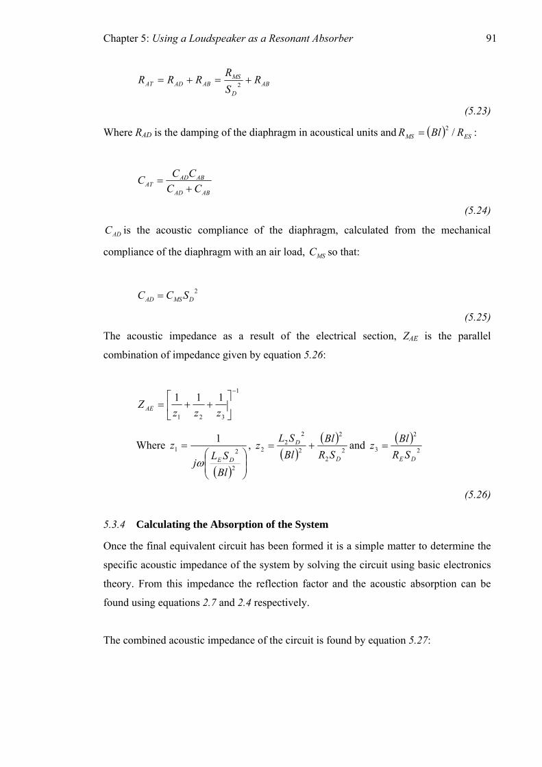
Chapter 5: Using a Loudspeaker as a Resonant Absorber 91
ABD
MSABADAT R
SR
RRR +=+= 2
(5.23)
Where RAD is the damping of the diaphragm in acoustical units and : ( ) ESMS RBlR /2=
ABAD
ABADAT CC
CCC+
=
(5.24)
is the acoustic compliance of the diaphragm, calculated from the mechanical
liance of the d
AD
comp
C
iaphragm with an air load, MSC so that:
2AC = DMSD SC
(5.25)
The acoustic impedance as a result of the electrical section, ZAE is the parallel
combination of impedance given by equation 5.26:
1
321
111⎥⎦
⎤⎢⎣
⎡++=
zzzZ AE
re
−
, ( )
( )2
2
2
2
22
2D
D
SRBl
BlSLz += and ( )
2
2
3DE SR
Blz =Whe
( ) ⎟⎟⎠
⎞⎜⎜⎝
⎛=
2
211
BlSLj
zDEω
(5.26)
5.3.4 Calculating the Absorption of the System
Once the final equivalent circuit has been formed it is a simple matter to determine the
eory. From this impedance the reflection factor and the acoustic absorption can be
ing equations 2.7 and 2.4 respectively.
The combined acous
specific acoustic impedance of the system by solving the circuit using basic electronics
th
found us
tic impedance of the circuit is found by equation 5.27:

Chapter 5: Using a Loudspeaker as a Resonant Absorber 92
AEAF ZZ ++ ATAT
ADTOT RCj
MjZ ++=ω
ω 1
stic impedance
f the system from which the absorption can be obtained.
5.4 Implementing the Model
The equivalent circuit model was implemented using MATLAB to plot the pre
abso
ode generate the results can be
und in Appendix J.
(5.27)
Multiplying this by a factor of the diaphragm area gives the specific acou
o
dicted
rption versus frequency of the driver. Figure 5.15 shows the predicted and
measured absorption on the same axes. The c used to
fo
50 100 150 200 250 300 350 4000
0.2
0.4
0.6
Using a Loudspeaker as an Absorber
1
0.8
Abs
orpt
ion
Coe
ffici
ent
Results from Impedance TubeEquivalent Circuit Prediction
Frequency, Hz
ood correlation between measurement and prediction is shown in terms of absorption
ver predict a
roader Q-factor of absorption than measurements show. This is due the limitations of
the lumped element modelling technique and results in difficulty in accurately
predicting the surface impedance of the system for all frequencies. Looking at the real
Figure 5.15 Comparison of equivalent circuit model with impedance tube measurements
5.4.1 Discussion
G
magnitude and resonant frequency. The equivalent circuit model does howe
b

Chapter 5: Using a Loudspeaker as a Resonant Absorber 93
part of the impedance (shown in Figure 5.16) for b elled
cases reveals that there is a dramatic increase in the real part of the measured surface
impedance at higher frequencies which is not present in the predicted data.
oth the measured and the mod
50 100 150 200 250 300 350 400 4500
500
Real Part of the Surface Impedance of a Loudspeaker used as an Absorber3000
2500
1000
1500
2000
Sur
face
Impe
danc
e
MeasuredPredicted
Frequency, Hz
Figure 5.16 Real part of surface impedance from both predicted and measured data
Accurate prediction of the losses in the system are shown at low frequency but the
accuracy decreases as the frequency increases, this explains why the predicted Q-factor
of the resonant curve is broader than the measured value. With the real part of the
measured impedance tending sharply away from characteristic impedance the system
reaches maximum absorption over only a narrow bandwidth which is contrasted with
the prediction where the real component of the impedance remains roughly equal to
characteristic impedance for the entire frequency range. The inaccuracy in the
aphragm that
annot be modelled using the lumped element method as it only predicts the
ce of systems. The first three modes of a circular plate can be given
prediction model is the result of secondary resonances of the driver di
c
fundamental resonan
as Figure 5.17 [38].

Chapter 5: Using a Loudspeaker as a Resonant Absorber 94
f01 f02
- + +-
f11
Figure 5.17 First three vibrational modes of a circular plate
The second modal frequency given by f11 is a resonant mode but will not generate any
absorption as there is cancellation on the diaphragm i.e. the diaphragm is ‘pushing’ and
‘pulling’ the same amount of air, consequently there is no resultant transmission of
energy and hence no absorption. It would therefore be expected that the imaginary part
of the surface impedance would exhibit a secondary point of zero crossin at this modal
frequency but which would show insignificant absorption, looking at Figure 5.18 this
becomes clear. The can at this modal frequency causes the real part of the
surface impedance to increase preventing efficient transmission, resulting in minimum
absorption as shown by Figure 5.18:
g
cellation
50 100 150 200 250 300 350 400 4500
0.5
1
Absorption Coefficient
α
50 100 150 200 250 300 350 400 4500
1000
2000
3000Real Impedance
Rea
l(z),
MK
S ra
yl
50 100 150 200 250 300 350 400 450-4000
-2000
0
2000
Imag
(z),
MK
Frequency, Hz
Absorption and Surface Impedance of a Loudspeaker Used as an Absorber
Imaginary Impedance
(a) (c) (b)
S ra
yl
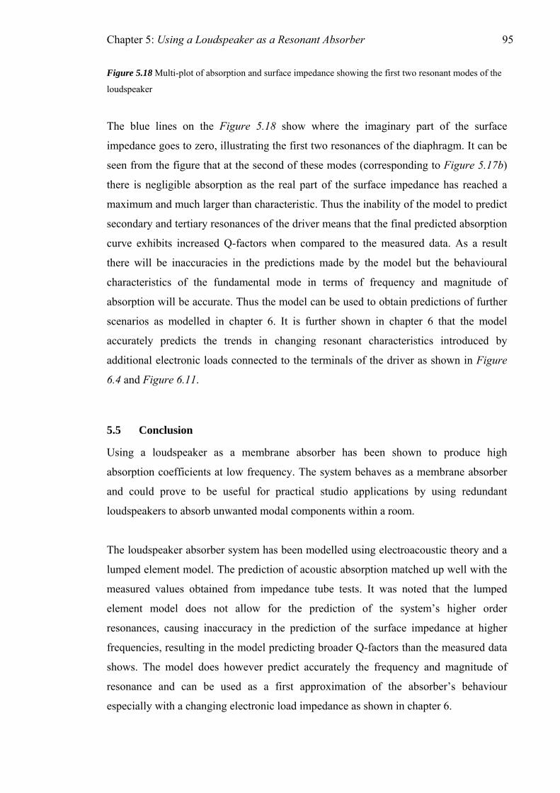
Chapter 5: Using a Loudspeaker as a Resonant Absorber 95
Figure 5.1 lti-plot of absorption and surface imped showing the first two resonant modes of the
loudspeaker
The blue lines on the Figure 5.18 show where the imaginary part of the surface
impedance goes to zero, illustrating the first two resonances of the diaphragm. It can be
seen f the figure that at the second of these modes (corresponding to Figure 5.17b)
there is negligible absorption as the real part of the surface impedance has reached a
aximum and much larger than characteristic. Thus the inability of the model to predict
5.5 Conclusion
Using a loudspeaker as a membrane absorber has been shown to produce high
absorption coefficients at low frequency. The system behaves as a membrane absorber
and could prove to be useful for practical studio applications by using redundant
loudspeakers to absorb unwanted modal components within a room.
The loudspeaker absorber system has been modelled using electroacoustic theory and a
lumped element model. The prediction of acoustic absorption matched up well with the
measured values obtained from impedance tube tests. It was noted that the lumped
element model does not allow for the prediction of the system’s higher order
resonances, causing inaccuracy in the prediction of the surface impedance at higher
frequencies, resulting in the model predicting broader Q-factors than the measured data
shows. The model does however predict accurately the frequency and magnitude of
resonance and can be used as a first approximation of the absorber’s behaviour
especially with a changing electronic load impedance as shown in chapter 6.
8 Mu ance
rom
m
secondary and tertiary resonances of the driver means that the final predicted absorption
curve exhibits increased Q-factors when compared to the measured data. As a result
there will be inaccuracies in the predictions made by the model but the behavioural
characteristics of the fundamental mode in terms of frequency and magnitude of
absorption will be accurate. Thus the model can be used to obtain predictions of further
scenarios as modelled in chapter 6. It is further shown in chapter 6 odel
accurately predicts the trends in changing resonant characteristics introduced by
additional electronic loads connected to the terminals of the driver as shown in
that the m
Figure
6.4 and Figure 6.11.

Chapter 5: Using a Loudspeaker as a Resonant Absorber 96
ection of work outlines how a passive electronic load on the driver can be
sed to reduce the resonant frequency and Q-factor of the loudspeaker absorber system.
The next s
u
The equivalent circuit model presented in this chapter will be extended to model such
changes in the motor impedance of the loudspeaker.
Chapter 6: Changing the Resonant Characteristics Using Passive Electronics 97
6. CHANGING THE RESONANT
CHARACTERISTICS OF A
LOUDSPEAKER-ABSORBER USING
PASSIVE ELECTRONICS
6.1 Introduction
The previous chapter outlined the basic principles of the modelling and use of a
loudspeaker used, in reverse, as an acoustic absorber. Sound incident to the diaphragm
of the loudspeaker, forces it into oscillation in sympathy to the frequency of the incident
wave causing a particle flow in the cabinet which is absorbed by porous material. The
system, as expected, was shown to have a distinct resonant peak, the frequency and
magnitude of which was controlled by the mechanical, acoustical and the electrical
components of the system. This was brought together in the form of a lumped parameter

Chapter 6: Changing the Resonant Characteristics Using Passive Electronics 98
m
an
odel which enabled prediction of the overall acoustic impedance of the system from
equivalent circuit, which in turn was used to determine the complex reflection factor
d hence the normal incidence absorption coefficient. This model was then compared
to tests performed in an impedance tube and was shown to accurately predict the
equency and magnitude of the system’s resonance.
the current chapter, the principles of the previous chapter are built upon such that
rameters concerning the system are changed in order to produce an absorber with
riable resonance characteristics. For a standard membrane absorber it is possible, if
not practical, to alter the mechanical and acoustical compliance, mass and damping
is is often very
impractical as it means altering physical properties such as the volume/depth of the
s demand a complete
ally
as
. Changing this electrical
coustic impedance of the
stem to be altered. The real part of the impedance, which determines the magnitude
d the Q-factor of absorption, can be altered by the addition of resistive components.
he imaginary part, which dictates the frequency of the resonance, can be altered by the
clusion of additional reactive components.
Altering acoustical properties of resonant systems with the use of electronic components
not a new idea; it has been applied to many areas including design of loudspeakers
with a better low frequency response [29]. In this case Stahl used electronic components
plifier thereby changing the impedance load as seen by the
reactive electronic components such that the resonant frequency and damping were
an
fr
In
pa
va
terms within the system to change its resonant characteristics. Th
cabinet or the material of the membrane. These change
reconstruction of the absorber so are not only time consuming but are also financi
costly. Using a loudspeaker as an absorber can provide a solution to this problem
there is the addition of an electrical domain in the system
section using variable components enables the combined a
sy
an
T
in
is
connected to an am
loudspeaker, Stahl noted that this caused the fundamental resonance to be altered and
enabled tuning to produce a better low frequency response. Stahl’s paper also
demonstrated a lumped element model to back up laboratory tests. This application was
focused on the radiation of sound but the theory of changing an electronic load to alter
an acoustic system has been applied also to the absorption of sound in the field of
aeroacoustics [39]. In this case a Helmholtz absorber was presented with a piezoelectric
backplate, the impedance of which could be varied by the addition of resistive and
Chapter 6: Changing the Resonant Characteristics Using Passive Electronics 99
altered. Results showed a shift in resonant frequency of up to 20% with the inclusion of
capacitive and inductive components. Resistive components could also be added and
were shown to alter the Q-factor of the resonance by the increase in damping. The
application for this study was in engine liners for aircraft where the frequency of noise
from the engine depends on the velocity of the aircraft therefore an absorber with
ariable characteristics is desirable.
celerometer on a loudspeaker) to actively
hange the resonance characteristics of a loudspeaker that was used passively to absorb
v
Using loudspeakers as absorbing systems has also been used extensively in room
acoustics with active absorption systems [40, 41] these systems use powered electronic
circuits and loudspeakers to cancel out incident sound by radiating a phase inverted
version of that sound which destructively interferes, absorbing the incident wave. It is
also possible to combine active and passive absorption techniques for room acoustic
applications [42]; this patented bass trap uses active control to tune a loudspeaker such
that it will passively absorb acoustic energy at it resonant frequency, Kashani and
Wischmeyer presented results displaying significant attenuation in a low frequency
band. The system allows two room modes to be absorbed simultaneously using this
active tuning. A further example of combining active and passive techniques is in the
field of space and rocket technology, where noise in the nose cone of a launch vehicle
can get to such large levels (exceeding 140dB) that damage can be inflicted on the
vehicle. Kemp and Clark [43] presented a technique combining a passive and active
control approach using an active input (an ac
c
the noise in the fairing (nose cone), they demonstrated peak reductions in excess of
12dB using this technique.
Both of the techniques mentioned above, using loudspeakers in the absorption of sound
use an active approach of tuning absorbers; however the absorber system presented here
does not utilise any active control but achieves high absorption coefficients over a range
of two and a half octaves using only passive techniques. As such this technique is an
extension of other methods available. In this work the resonant frequency can be altered
to allow the absorber to be transferred from room to room and retuned to match the
fundamental m e of that room. The magnitude and Q-factor of the absorption curve
can also be altered with the aim of smoothing out the frequency response. Of primary
interest is the effect of a single load resistance or capacitance, these will therefore be
od

Chapter 6: Changing the Resonant Characteristics Using Passive Electronics 100
described first. However the complex load impedance connected to the terminals of the
loudspeaker could potentially contain any combination of resistive and reactive
components to produce the optimum resonant characteristics for a given application and
more complex arrangements will hence be analysed in subsequent sections.
Changing the resistive element of the impedance presented to the terminals A and B of
e loudspeaker used as an absorber was analysed first.
.2.1 Theory and Prediction
th
6.2 Changing the Load Resistance
It is useful in applications to be able to determine the Q-factor of the absorption
provided by a membrane absorber, the advantage can be seen in two ways. Firstly if the
Q-factor is decreased it enables an increased bandwidth of absorption, something highly
sought after in room acoustics, to result in a room with a flatter response with respect to
frequency over a wider bandwidth. Secondly if the Q-factor could be increased it allows
more selectivity with the frequencies that the system could absorb, such that if there was
a problem with increased modal excitation at a discrete frequency it could be selectively
absorbed without effecting neighbouring frequencies. Varying the load resistance will
be elucidated in the subsequent section altering the Q of the resonance by a degree of
34% allowing for the user to select the Q-factor within certain bounds for the
application of choice. There is also the possibility of applying a negative resistance
across the terminals to decrease the Q-factor still further but this would require an
additional power source and falls outside the scope of this project.
6
The lumped element model derived in the previous chapter was extended here to allow
the modelling of additional passive electronic components in the electrical section of the
analogue. With the additional variable resistance, REV, the electrical section of the
equivalent circuit as modelled with the impedance analogue then becomes as Figure
6.1:
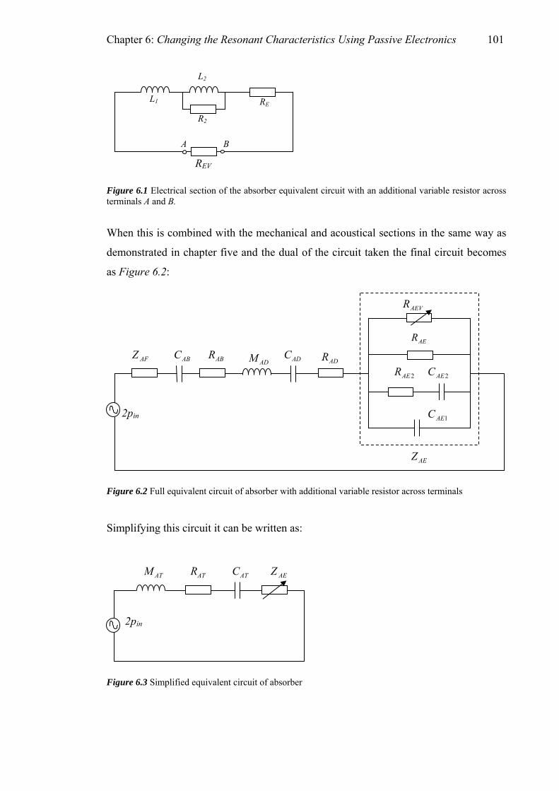
Chapter 6: Changing the Resonant Characteristics Using Passive Electronics 101
A B
RE L1
L2
R2
Figure 6.1 Electrical section of the absorber equivalent circuit with
REV
an additional variable resistor across als A and B.
l and acoustical sections in the same way as
demonstrated in chapter five and the dual of the circuit taken the final circuit becomes
ross terminals
Figure 6.3 Simplified equivalent circuit of absorber
termin
When this is combined with the mechanica
as Figure 6.2:
Figure 6.2 Full equivalent circuit of absorber with additional variable resistor ac
Simplifying this circuit it can be written as:
ATM ATR ATC AEZ
2pin
2pin
AFZ ADC ADM ADR ABR
AEVR
AER
2AER 2AEC
1AEC
AEZ
ABC
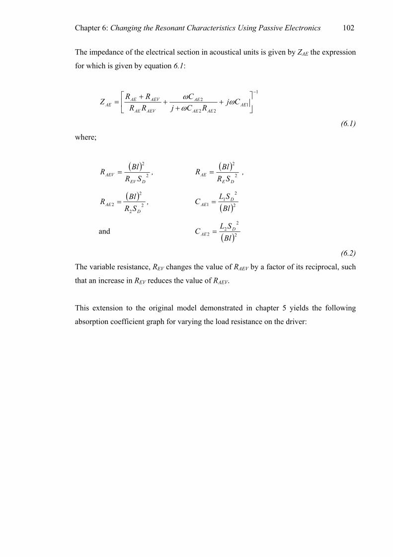
Chapter 6: Changing the Resonant Characteristics Using Passive Electronics 102
The impedance of the electrical section in acoustical units is given by ZAE the expression
for which is given by equation 6.1
:
1
122
2
−
⎥⎦
⎤⎢⎣
⎡+
++
+= AE
AEAE
AE
AEE R VA
AEAE Cj
RCjC
RRR
Z ωωω
(6.1)
AE V
where;
( )2
2
DEVAEV SR
BlR = , ( )2
2
DEAE SR
BlR = ,
( )2
2
2
2D
AE SRBlR = ,
( )2
21
1 BlSLC D
AE =
( )2
22
2 BlSLC D
AE =and
(6.2)
The variable resistance, REV changes the value of RAEV by a factor of its reciprocal, such
that an increase in REV reduces the value of RAEV.
This extension to the original model demonstrated in chapter 5 yields the following
absorption coefficient graph for varying the load resistance on the driver:

Chapter 6: Changing the Resonant Characteristics Using Passive Electronics 103
100 200 300 400 500 600 7000
0.2
0.4
0.6
0.8
1
Frequency, Hz
Abs
orp
Predicted Absorption Coefficients with Varying Resistive Load
Closed Circuit1 Ohm5 Ohms10 Ohms50 Ohms100 OhmsOpen Circuit
tion
Coe
ffici
ent
Figure 6.4 Changes in absorption curves with a variable resistor connected across loudspeaker terminals
states that additional resistance adds
amping to the circuit and should therefore reduce the Q-factor rather than increase it.
e in the load
resistance actually increases the conductance in acoustical units.
The variations in Q-factor are governed by the open and closed circuit limiting
conditions. The closed circuit offers the minimum load resistance and the open circuit
case offers the highest possible load resistance, thus these conditions define the
minimum and maximum Q-factors obtainable with standard linear electrical resistors.
6.2.2 Measurements
Measurements were made using the specially constructed impedance tube in the same
manner as in chapter 5. The electrical load resistance applied to the terminals of the
driver was altered for each measurement using a standard variable resistance box with a
maximum error of 0.1% verified with a digital multi-meter. In order to connect the
This prediction shows that the Q-factor of the absorption curve rises with an increase in
load resistance; this is counter to intuition which
d
The reason for this is that the final analogue is written in the impedance analogue such
that electrical resistances actually become conductances, so an increas

Chapter 6: Changing the Resonant Characteristics Using Passive Electronics 104
resistance box to the terminals of the driver, wires had to be fed from the driver under
the mounting rings shown in Figure 6.5:
igure 6.5 Mounting of loudspeaker in large sample holder for impedance tube testing
he sample holder; this
as done so that the Q-factor would be higher in order that the effect of the changing
Mounting rings
Loudspeaker
Wires fed under mounting rings
Terminals to connect passive electronics to
F
Care had to be taken to avoid any leaks between the mounting rings and the top of the
sample holder so as to prevent spurious results. This was achieved by using Blu-tak to
block any gaps.
Initial measurements were made with no porous absorbent in t
w
resistance could be more clearly discernable. On subsequent analysis it was found that
these measurements did not match up well with predictions. The absorption coefficient
curves that were obtained are seen in Figure 6.6:
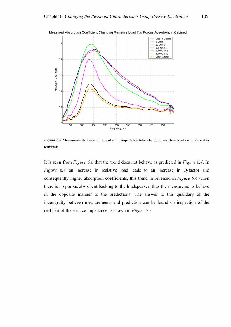
Chapter 6: Changing the Resonant Characteristics Using Passive Electronics 105
50 100 150 200 250 300 350 400 4500
0.2
0.4
0.6
0.8
1
Frequency, Hz
Abs
orpt
ion
Coe
ffici
ent
Measured Absorption Coefficient Changing Resistive Load [No Porous Absorbent in Cabinet]
Closed Cicruit1 Ohm10 Ohms100 Ohms1000 Ohms5000 OhmsOpen Circuit
Figure 6.6 Measurements made on absorb r in impedance tube changing resistive load on loudspeaker
her absorption coefficients, this trend in reversed in Figure 6.6 when
ere is no porous absorbent backing to the loudspeaker, thus the measurements behave
e
terminals
It is seen from Figure 6.6 that the trend does not behave as predicted in Figure 6.4. In
Figure 6.4 an increase in resistive load leads to an increase in Q-factor and
consequently hig
th
in the opposite manner to the predictions. The answer to this quandary of the
incongruity between measurements and prediction can be found on inspection of the
real part of the surface impedance as shown in Figure 6.7.
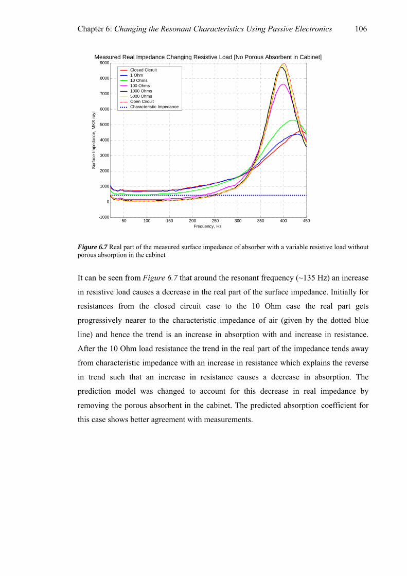
Chapter 6: Changing the Resonant Characteristics Using Passive Electronics 106
50 100 150 200 250 300 350 400 450-1000
0
1000
2000
3000
4000
5000
6000
7000
8000
9000
Frequency, Hz
Sur
face
Impe
danc
e, M
KS
rayl
Measured Real Impedance Changing Resistive Load [No Porous Absorbent in Cabinet]
Closed Cicruit1 Ohm10 Ohms100 Ohms1000 Ohms5000 OhmsOpen CircuitCharacteristic Impedance
Figure 6.7 Real part of the measured surface impedance of absorber with a variable resistive load without porous abs
orption in the cabinet
can be seen from Figure 6.7 that around the resonant frequency (~135 Hz) an increase
e in absorption. The
prediction model was changed to account for this decrease in real impedance by
removing the porous absorbent in the cabinet. The predicted absorption coefficient for
this case shows better agreement with measurements.
It
in resistive load causes a decrease in the real part of the surface impedance. Initially for
resistances from the closed circuit case to the 10 Ohm case the real part gets
progressively nearer to the characteristic impedance of air (given by the dotted blue
line) and hence the trend is an increase in absorption with and increase in resistance.
After the 10 Ohm load resistance the trend in the real part of the impedance tends away
from characteristic impedance with an increase in resistance which explains the reverse
in trend such that an increase in resistance causes a decreas
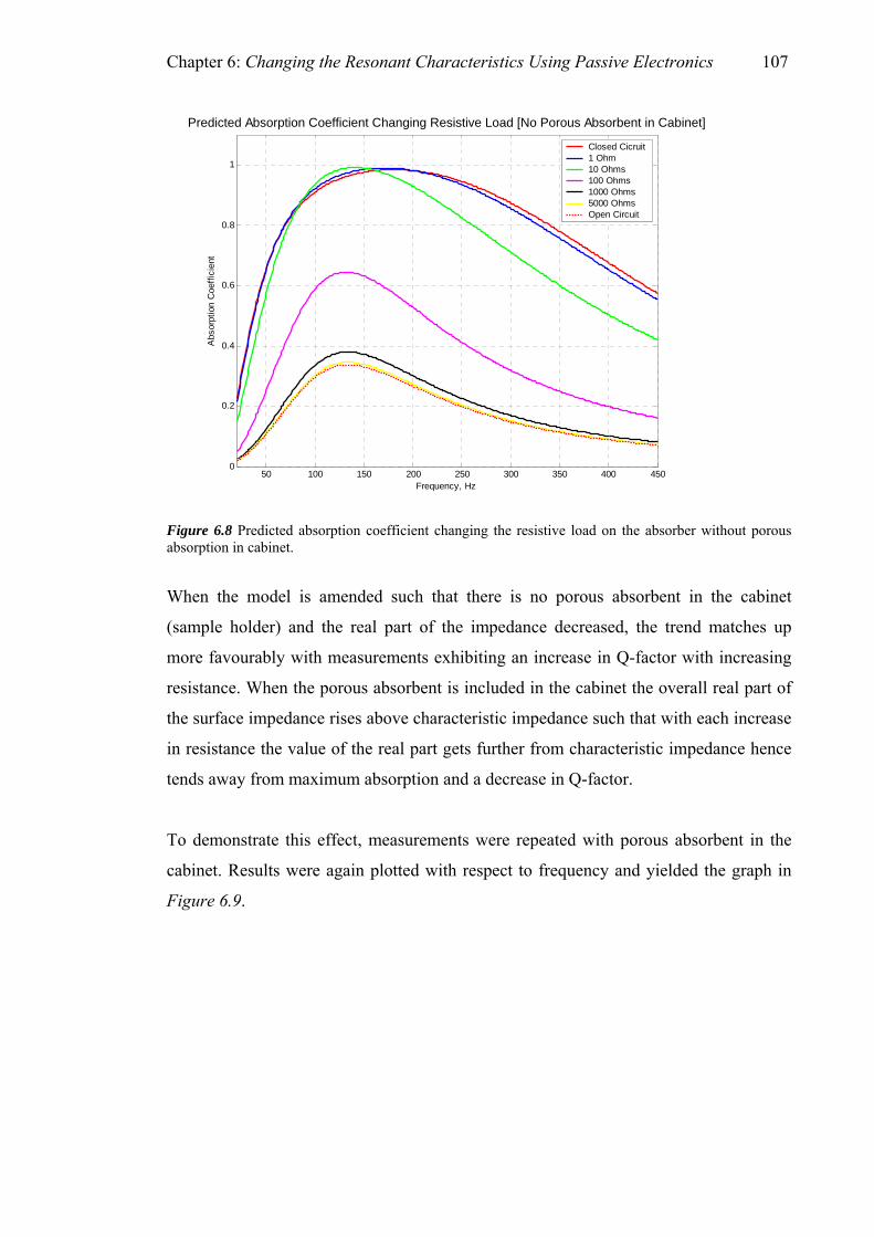
Chapter 6: Changing the Resonant Characteristics Using Passive Electronics 107
50 100 150 200 250 300 350 400 4500
0.2
0.4
0.6
0.8
1
Frequency, Hz
Abs
orpt
ion
Coe
ffici
ent
Predicted Absorption Coefficient Changing Resistive Load [No Porous Absorbent in Cabinet]
Closed Cicruit1 Ohm10 Ohms100 Ohms1000 Ohms5000 OhmsOpen Circuit
Figure 6.8 Predicted absorption coefficient changing the resistive load on the absorber without porous absorption in cabinet.
amended
When the model is such that there is no porous absorbent in the cabinet
(sample holder) and the real part of the impedance decreased, the trend matches up
more favourably with measurements exhibiting an increase in Q-factor with increasing
resistance. When the porous absorbent is included in the cabinet the overall real part of
the surface impedance rises above characteristic impedance such that with each increase
in resistance the value of the real part gets further from characteristic impedance hence
tends away from maximum absorption and a decrease in Q-factor.
To demonstrate this effect, measurements were repeated with porous absorbent in the
cabinet. Results were again plotted with respect to frequency and yielded the graph in
Figure 6.9.

Chapter 6: Changing the Resonant Characteristics Using Passive Electronics 108
1
0.8
0.6
0.4
50 100 150 200 250 300 350 400 4500
0.2
Measured Absorption for Different Resistive Loads [With Porous Absorbent in Cabinet]
Frequency, Hz
Abs
orpt
ion
Coe
ffici
ent
Closed Circuit1 Ohms5 Ohms10 Ohms50 Ohms100 OhmsOpen Circuit
Figure 6.9 Measured absorption coefficient of absorber with variable resistive load with porous absorption in the cabinet
here is a slight shift in resonant frequency that is shown in both the measured and the
f the electrical section ZAEV. Expanding equation 6.1 shows that RAEV
ecomes a factor of the
This measurement shows good agreement with the predicted values plotted in Figure
6.4 confirming the validity of the model. Graphs with both the measured and predicted
results plotted on the same axes for each individual resistive load can be found in
Appendix K. The model, as mentioned in section 5.4.1, tends to slightly over predict the
Q-factor of the resonance but as will be seen in section 6.5.2 the trend of how the Q-
factor changes with increasing resistive loads is accurately predicted.
T
predicted data, the resonant frequency decreasing slightly with the additional resistive
load. The reason for this shift is found when analysing the combined complex
impedance o
1AECω and 2AECωb therefore changing the resistive load will
have an effect on the magnitude of the reactive parts and consequently on the resonant
frequency of the system. This effect is small when compared with the fundamental
resonance frequency with the closed circuit case; the shift is from 142 to 132Hz a shift
of just 7%. Greater shifts in resonant frequency can be obtained if a capacitor is
introduced into the circuit as seen in section 6.2.3.

Chapter 6: Changing the Resonant Characteristics Using Passive Electronics 109
6.2.3 Summary
Changing the resistive load has been shown to have different effects on the Q-factor of
the resonant peak of absorption in the loudspeaker absorber system. The effect depends
on the initial magnitude of the real part of the surface impedance. It has been shown that
of the real impedance is above characteristic impedance for the closed circuit case then
the trend is an increase in Q-factor and absorption with an increase in resistance as with
each addition of resistance the real surface impedance of the system gets progressively
closer to characteristic impedance of air and hence maximum absorption at resonance.
The trend is reversed if the real part is initially below characteristic impedance for the
closed circuit case, as with each addition of resistance the value at resonance tends away
from characteristic impedance resulting in a decrease in absorption and Q-factor with
increase in resistance.
When designing a resonant absorber of this type it will be useful to change the Q-factor
lectively absorb discrete frequencies to a certain degree to achieve
e flattest possible room response with respect to frequency. Section 6.5 will outline
ker it is possible
lso to include the addition of reactive components, in this section a variable capacitor
e absorber system will behave with
hanging load capacitance can be made. Thus the new circuit becomes:
of the resonance to se
th
some useful equations and graphs that could be used to determine what resistive value
should be used to achieve a given Q-factor for a specific driver.
6.3 Changing the Capacitive Load
As well as adding a variable resistor to the terminals of the loudspea
a
was included in the circuit. The desired outcome of this was the lowering of the
system’s resonant frequency. Experiments were performed in the impedance tube and
the scenario modelled using the standard equivalent circuit approach as in previous
sections. Measurements showed that shifts in resonant frequency of up to 39% were
possible with the addition of a single capacitor.
6.3.1 Theory and Prediction
Adding a capacitor into the circuit in Figure 5.13 leads to the equivalent circuit shown
in Figure 6.10 from which predictions of how th
c

Chapter 6: Changing the Resonant Characteristics Using Passive Electronics 110
Figure 6.10 Equivalent circuit with additional variable capacitor connected to loudspeaker terminals
In this case:
( )
2
2
D
EVAEV S
BlCL =
(6.3)
Increasing the variable capacitor CEV consequently increases the value of the variable
ductor LAEV. Using the adapted circuit and computing the surface impedance yields the
ure 6.11.
in
absorption coefficient curves shown Fig
50 100 150 200 250 300 350 4000
0.2
0.4
0.6
0.8
1
Frequency, Hz
Abs
orpt
ion
Coe
ffici
ent
Predicted Absorption Coefficients with Varying Capacitive Load
Closed Circuit1μF10μF22μF47μF100μF220μF470μFOpen Circuit
AFZ ADC ADM ADR ABR
AEVL
AER
2AER 2AEC
1AEC
AEZ
ABC
2pin

Chapter 6: Changing the Resonant Characteristics Using Passive Electronics 111
Figure 6.11 Predicted absorption curves with a variable capacitor connected to loudspeaker terminals
The graph shows a decrease in resonant frequency with an increase in capacitive load.
Results from the equivalent circuit model suggest that there is an optimum capacitance
where by increasing the capacitance further will begin to increase the resonant
frequency until once again it resonates at the same fr ed circuit case.
The model predicts a resonant frequency shift of some 51% with the system resonating
at 174Hz for the closed circuit case and 85Hz with a 220μF load capacita
6.3.2 Measurements
Measurements were once again performed in the low frequency impedance tube. The
ost
portant case if the absorber were to be used in a practical setting. Standard electrical
apacitors were used in the measurements with capacities ranging from 1-
470μF. esults yielded th
equency as the clos
nce.
results were made with porous absorbent material in the cabinet as this is the m
im
component c
R e following Figure 6.12.
50 100 150 200 250 300 350 4000
0.2
0.4
0.6
0.8
1
Frequency, Hz
Abs
orpt
ion
Coe
ffici
ent
Measured Absorption Coefficients with Varying Capacitive Load
Closed Circuit1μF10μF22μF47μF100μF220μF470μFOpen Circuit
Figure 6.12 Measured absorption curves, changing the load capacitance connected across loudspeaker terminals

Chapter 6: Changing the Resonant Characteristics Using Passive Electronics 112
Results from the measurements show a similar trend to the predictions such that an
increase in capacitive load leads to a decrease in the system’s resonant frequency. The
lowest frequency was found with a capacitance of 100 μF. The prediction model and the
measurements show that if the capacitance is increased too much then resonant
frequency increases again. The high frequency limit is given by the closed circuit
condition. The measured results show a resonant frequency shift from 172Hz to 105Hz
which corresponds to a shift of 39% which is slightly less than predicted due to
limitations in the lumped element method of analysis mentioned in section 5.4.1.
6.3.3 Discussion
Results show that with the addition of the reactive component there appears to still be
some resistive losses added into the system manifesting as a reduction in the Q-factor of
the resonance peak. This is due to the construction of the circuit, namely the t the
uit
f the absorber, it is seen that in the final analogue circuit, what was electrically in
he lowest
ossible frequency, a trade off has to be made. As more resistance is added the resonant
d less by the reactive component as the resistive component
becomes the dominant term in controlling the motor impedance.
%. A maximum value of capacitance
was found, a value above which would begin to increase the resonant frequency again.
The optimum capacitance in the model was 220μF where as in measurements was
100μF. This value is subject to change given a specific driver; this is the topic of section
6.5.1. Increasing the capacitance, as well as lowering the resonant frequency, also
fact tha
components are connected to the voice coil in series. Looking at the equivalent circ
o
series becomes in parallel in the final model. Combining the complex impedances in
parallel means that the resistive components have impact on the frequency and that
reactive components have an impact on resistive losses, such that the resistive
components become multipliers of frequency dependent terms and capacitors become
multipliers of resistive terms. This means that when trying more complex scenarios such
as adding additional resistive components to achieve high absorption at t
p
frequency can be shifte
6.3.4 Summary
By adding a capacitive load to the terminals of the driver it has been shown that it is
possible to achieve a resonant frequency shift of 39

Chapter 6: Changing the Resonant Characteristics Using Passive Electronics 113
increases the Q-factor of the resonance curve thus there is a trade off between obtaining
the lowest possible frequency of a given system and obtaining maximum absorption.
6.4 Modelling Other Scenarios
So far it has been shown that by adding a variable resistance or capacitance into the
circuit the loudspeaker absorber can be tuned to exhibit different resonant
characteristics such that the Q-factor and the resonant frequency can be altered. A
variable resistor and capacitor constitute the simplest cases of adding both singular
resistive and reactive components. In this next section further scenarios are modelled
using the equivalent circuit model. Being able to change the resonant frequency of the
system is very useful but it is to the detriment of absorption magnitude at resonance.
More complicated combinations of electronic components could present an optimum
situation where the lowest resonant frequency could be achieved but yet exhibit
maximum absorption. Several combinations of additional electronic components are
modelled in this section; firstly, resistors and capacitors in series and in parall ,
apacitive and inductive elements both in series and in parallel.
el
secondly, the addition of an inductive component and thirdly, the combination of
c
6.4.1 Resistors and Capacitors in Series
In order to see if there is a greater degree of tunability available with the loudspeaker
absorber system it was seen what would happen if a variable resistor was placed with a
variable capacitor in series, in the final equivalent circuit these appear as a variable
inductor and conductance in parallel with the other motor impedance terms, the
equivalent in this case is given by Figure 6.13:

Chapter 6: Changing the Resonant Characteristics Using Passive Electronics 114
Figure 6.13 Equivalent circuit modelling a variable resistor in series with a variable capacitor connected to the terminals of the loudspeaker
It was hoped that the addition of the extra variable resistor in series with the variable
capacitor would allow the system to resonate at the lowest possible frequency, as
governed by the capacitor whilst having the maximum absorption coefficient at
resonance, governed by the variable resistor. This turned out not to be the case as was
seen when plotting the absorption coefficient versus frequency for varying capacitive
and resistive loads. A multi-plot demonstrating how the trend in absorption changes
with differing combinations of resistive and capacitive loads in series is shown in
Figure 6.14.
AFZ ATM ATR AER
2AER 2AEC
1AEC
AEVR
AEVL
ATC
2pin
AEZ

Chapter 6: Changing the Resonant Characteristics Using Passive Electronics 115
1 Ω 5 Ω 10 ΩPredicted Absorption Curves, Varying Load Capacitance and Resistance
100 200 300 4000
0.2
0.4
0.6
0.8
1
Freq, Hz
α
100 200 300 4000
0.2
0.4
0.6
0.8
1
100 200 300 4000
0.2
1
0.8
0.6
Freq, Hz
α
0.4
α
Freq, Hz
100 200 300 4000
0.2
0.4
0.6
0.8
1
Freq, Hz
α
50 Ω
100 200 300 4000
0.2
0.4
0.6
0.8
1
Fre Hz
α
q,
100 Ω
100 200 300 4000
0.2
0.4
0.6
0.8
1
Freq, Hz
α
500 Ω
1 μF 10 μF 22 μF 47 μF100 μF220 μF470 μF
Figure 6.14 Multi-plot showing changes in the trend of absorption for d t c binations of resistors in series with capacitors
It can be seen from Figure 6.14, that a change in load resistance on the driver
suppresses the effect of the change in capacitance to increasing amounts with an
increase in resistance. Thus using a capacitor and resistor in series does not have the
desired effect of lowest frequency absorption with maximum absorption coefficient. To
ecreases according to equation 6.2, thus current will flow
ing to increase the adaptability of the resonant absorber.
ifferen om
discern the reason for it is helpful to look at the equivalent circuit in Figure 6.13. As the
alue of REV increases RAEV dv
more easily through that branch of the circuit. Consequently as RAEV decreases, less
current flows through LAEV and the circuit tends towards the case with no variable
capacitance at all, i.e. the equivalent circuit becomes as Figure 6.2. As the resistance is
then very high it tends towards the open circuit case as results show in Figure 6.14.
Therefore with a higher load resistance the change in load capacitance makes
continually less difference to the resonant characteristics of the system. Consequently
the simple series connection of a single resistor and capacitor does not constitute a
useful case when aim
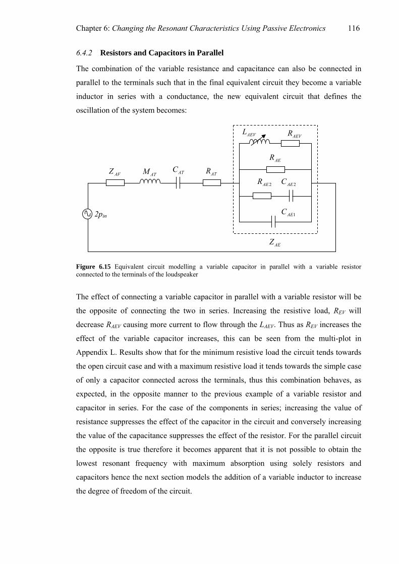
Chapter 6: Changing the Resonant Characteristics Using Passive Electronics 116
6.4.2 Resistors and Capacitors in Parallel
The combination of the variable resistance and capacitance can also be connected in
parallel to the terminals such that in the final equivalent circuit they become a variable
inductor in series with a conductance, the new equivalent circuit that defines the
oscillation of the system becomes:
s of the loudspeaker
increase
e degree of freedom of the circuit.
AFZ ATM ATR
AEVL
AER
2AER 2AEC
1AEC
AEZ
ATC
2pin
AEVR
Figure 6.15 Equivalent circuit modelling a variable capacitor in parallel with a variable resistor connected to the terminal
The effect of connecting a variable capacitor in parallel with a variable resistor will be
the opposite of connecting the two in series. Increasing the resistive load, REV will
decrease RAEV causing more current to flow through the LAEV. Thus as REV increases the
effect of the variable capacitor increases, this can be seen from the multi-plot in
Appendix L. Results show that for the minimum resistive load the circuit tends towards
the open circuit case and with a maximum resistive load it tends towards the simple case
of only a capacitor connected across the terminals, thus this combination behaves, as
expected, in the opposite manner to the previous example of a variable resistor and
capacitor in series. For the case of the components in series; increasing the value of
resistance suppresses the effect of the capacitor in the circuit and conversely increasing
the value of the capacitance suppresses the effect of the resistor. For the parallel circuit
the opposite is true therefore it becomes apparent that it is not possible to obtain the
lowest resonant frequency with maximum absorption using solely resistors and
capacitors hence the next section models the addition of a variable inductor to
th

Chapter 6: Changing the Resonant Characteristics Using Passive Electronics 117
6.4.3 Applying an Variable Inductor
If a variable inductor is added in series into the circuit it manifests itself as a variable
capacitor in parallel with the voice coil impedance terms in addition to the final
equivalent circuit Figure 5.15. The circuit that defines this condition then becomes as
Figure 6.16:
AFZ
Figure 6.16 Equivalent circuit modelling a variable inductor connected to the terminals of the loudspeaker
Where
( )2
2
BlSL
C DEVAEV = ,
AEVC Cj
ZAEV ω
1=
(6.4)
Plotting the predicted absorption from this equivalent circuit yields Figure 6.17.
ATM ATR AER
2AER 2AEC
1AEC
AEZ
ATC
2pin
AEVC

Chapter 6: Changing the Resonant Characteristics Using Passive Electronics 118
50 100 150 200 250 300 350 400 4500
0.2
0.4
0.6
0.8
1
Frequency, Hz
Abs
orpt
ion
Coe
ffici
ent
with Varying Inductive LoadPredicted Absorption Coefficients
0.5 mH 1 mH 5 mH 10 mH 50 mH 100 mH 500 mH1000 mH
Figure 6.17 Absorption curves changing inductive load on loudspeaker
ccording to equation 6.4, it can therefore be ignored for subsequent circuit analysis.
uently current only flows through the other three parallel branches thus the
circuit can be approxi ed onal passive
electronics. Conversely if LAEV is large the impedance of CAEV becomes very small
resulting in very little flow through the voice coil terms CAE1, CAE2, RAE2 and RAE. I
that the
motor impedance has no effect on the resonant characteristics of the absorber. These
situations govern the limits of the setup. Figure 6.17 demonstrates that with large
inductances the circuit behaves as the closed circuit case and with small inductances as
the open circuit case, intermediate inductance values cause frequency shifts in between
these values in a similar way to using a capacitor. It is also possible obtain a higher
resonant frequency than governed by the closed circuit condition where using a 10mH
inductor causes a resonant frequency of 197Hz with an absorption coefficient of 0.96.
The use of an inductor connected to the terminals of the loudspeaker consequently
enables higher resonant frequencies but still achieving high absorption coefficients, it
could therefore be profitable to combine more than one reactive component in order to
achieve a wider bandwidth of absorption.
When the load inductance LAEV is small the impedance of CAEV becomes very large
a
Conseq
mated by the clos circuit case with no additi
n this
case ZAE tends to zero thus the circuit approximates to the open circuit case such

Chapter 6: Changing the Resonant Characteristics Using Passive Electronics 119
6.4.4 A Variable Inductor and Capacitor in Series
In this section a variable inductor was modelled as connected in series with a variable
capacitor, the equivalent circuit for this scenario is given by Figure 6.18. Utilising an
inductor and a capacitor it was hoped that the advantages of both types of component
could be exploited, the capacitor enabling lower frequency limits and the inductor
enabling higher frequency limits, thus increasing the range of resonant frequencies.
Figure 6.18 Equivalent circuit modelling a variable inductor in series with a variable capacitor connected to the terminals of the loudspeaker
With two reactive components in the circuit it is expected to have two resonances
governed by the component values, as the passive electronic load now has an additional
degree of freedom. Figure 6.19 shows that this is the case with two resonant peaks
when using a variable inductor in series with a variable capacitor. Using a large enough
inductor means that the two resonant peaks occur in a similar frequency band such that
the inductor enhances the low frequency effect of the capacitor. This additional degree
of freedom provided by the inductor means that an increased range of frequencies can
be obtained.
AFZ ATM ATR
2AER 2AEC
1AEC
AEVL
AEVC
AEZ
ATC AER
2pin
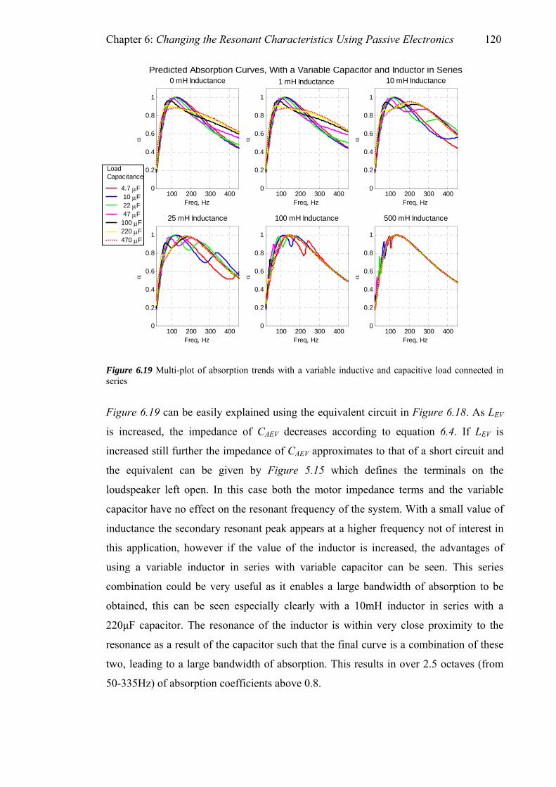
Chapter 6: Changing the Resonant Characteristics Using Passive Electronics 120
100 200 300 4000
0.2
0.4
0.6
0.8
1
Freq, Hz
α
0 mH Inductance
100 200 300 4000
0.2
0.4
0.6
Predicted Absorption Curves, With a Variable Capacitor an
0.8
1
Freq, Hz
α
1 mH Inductance
100 200 300 4000
0.2
0.4
0.6
0.8
1
Freq, Hz
α
10 mH Inductanced Inductor in Seri
Load Capacitance
4.7 μF 10 μF 22 μF
100 200 300 4000
0.2
0.4
0.6
0.8
1
Freq, Hz
α
25 mH Inductance 47 μF100 μF220 μF470 μF
100 200 300 4000
0.2
0.4
0.6
0.8
1
Freq, Hz
α
100 mH Inductance
100 200 300 4000
0.2
0.4
0.6
0.8
1
Fre z
α
500 mH Inductance
q, H
es
Figure 6.19 Multi-plot of absorption trends with a variable inductive and acitive load connected in series
Figure 6.19 can be easily explained using the equivalent circuit in Figure 6.18. As LEV
is increased, the impedance of CAEV decreases according to equation 6.4. If LEV is
by Figure 5.15 which defines the terminals on the
e motor impedance terms and the variable
capacitor such that the final curve is a combination of these
ing to a large bandwidth of absorption. This results in over 2.5 octaves (from
50-335Hz) of absorption coefficients above 0.8.
cap
increased still further the impedance of CAEV approximates to that of a short circuit and
the equivalent can be given
loudspeaker left open. In this case both th
capacitor have no effect on the resonant frequency of the system. With a small value of
inductance the secondary resonant peak appears at a higher frequency not of interest in
this application, however if the value of the inductor is increased, the advantages of
using a variable inductor in series with variable capacitor can be seen. This series
combination could be very useful as it enables a large bandwidth of absorption to be
obtained, this can be seen especially clearly with a 10mH inductor in series with a
220μF capacitor. The resonance of the inductor is within very close proximity to the
resonance as a result of the
two, lead
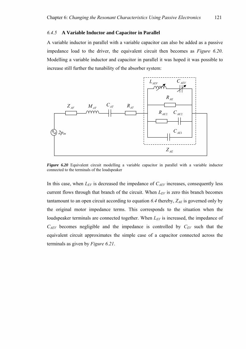
Chapter 6: Changing the Resonant Characteristics Using Passive Electronics 121
6.4.5 A Variable Inductor and Capacitor in Parallel
A variable inductor in parallel with a variable capacitor can also be added as a passive
impedance load to the driver, the equivalent circuit then becomes as Figure 6.20.
Modelling a variable inductor and capacitor in parallel it was hoped it was possible to
increase still further the tunability of the absorber system:
ted to the terminals of the loudspeaker
AFZ ATM ATR
AEVL
AER
2AER 2AEC
1AEC
AEZ
ATC
2pin
AEVC
Figure 6.20 Equivalent circuit modelling a variable capacitor in parallel with a variable inductor connec
In this case, when LEV is decreased the impedance of CAEV increases, consequently less
current flows through that branch of the circuit. When LEV is zero this branch becomes
tantamount to an open circuit according to equation 6.4 thereby, ZAE is governed only by
the original motor impedance terms. This corresponds to the situation when the
loudspeaker terminals are connected together. When LEV is increased, the impedance of
CAEV becomes negligible and the impedance is controlled by CEV such that the
equivalent circuit approximates the simple case of a capacitor connected across the
terminals as given by Figure 6.21.

Chapter 6: Changing the Resonant Characteristics Using Passive Electronics 122
0 mH Inductance 1 mH InductancePredicted Absorption Curves, With a Variable Capacitor a
100 200 300 4000
0.2
0.4
0.6
0.8
1
Freq, Hz
α
100 200 300 4000
0.2
0.4
0.6
0.8
1
Freq, Hz
α
100 200 300 4000
0.2
0.4
0.6
0.8
1
Freq, Hz
10 mH Inductance
α
100 200 300 4000
0.2
0.4
0.6
0.8
1
Freq, Hz
α
25 mH Inductance
100 200 300 4000
0.2
0.4
0.6
0.8
1
Freq, Hz
α
100 mH Inductance
100 200 300 4000
0.2
0.4
0.6
0.8
1
Freq, Hz
α
500 mH Inductance
4.7 μF 10 μF 22 μF 47 μF100 μF220 μF470 μF
nd an Inductor in Parallel
Capacitance
speaker
inductor has been seen to provide a very significant
hift in resonant frequency and as such could be very useful in the creation of a versatile
membrane absorber for room acoustic applications.
6.4.6 Summary
Section 6.4 has demonstrated several complex electrical impedance loads that could be
connected to the terminals of the loudspeaker-absorber to increase its adaptability. Four
special cases can hence be outlined with distinct advantages in the absorption of sound.
Load
Figure 6.21 Multi-plot showing predicted absorption trends with a variable inductor and capacitor connected in parallel to the terminals of the loud
Results show that by using a capacitor in parallel with an inductor enables a lower
resonant frequency than simply using a capacitor on its own. The optimally low
resonant frequency is seen when a 25mH inductor is connected in parallel with a 470μF
capacitor, this demonstrates a resonant frequency of 65Hz, with an absorption
coefficient in excess of 0.85. The maximum resonant frequency obtained using this
technique is 223Hz, this corresponds to a maximum resonant frequency shift of 70%.
Using a capacitor in parallel with an
s

Chapter 6: Changing the Resonant Characteristics Using Passive Electronics 123
Firstly, simply adding a capacitor to the terminals has the effect of lowering the
system’s overall resonant frequency. This resonant frequency can then be reduced and
indeed increased further by the addition of an inductor in parallel, increasing the degree
of freedom of the system and allowing for a greater range of resonant frequencies to be
obtained. Thirdly connecting a resistor across the terminals of the loudspeaker alters the
Q-factor of the resonance, a decrease in resistive load increasing the Q-factor. This is
important as it defines how much acoustic energy the absorber will absorb at the chosen
frequency. The final important case is that of an inductor connected in series with a
capacitor, this is an important case as it results in a broad bandwidth of absorption,
something keenly sort after by the room acoustician.
Further scenario’s of electronic load impedances could also be modelled using more
than two reactive and resistive components to create more complex resistive loads thus
optimising the absorber for the required task but of primary concern here is the simple
case of up to two reactive and resistive components shown in the four important
e
omponent load. This is the first step towards an automated system which could
tic in a room and some intelligent
ardware could change a combination of electronic components connected to the
ly, such that the absorption characteristics were optimum for that
absorber.
scenario's above.
6.5 Optimising the Passive Electronic Load for a Given Set of Driver Parameters
In order to be able to fine tune the absorber system such that it achieves maximum
absorption at a set resonant frequency or with a specified Q-factor it is important to
ascertain what component values must be used in order to achieve the desired results.
This section outlines methods of determining capacitance and resistance values to be
able to achieve specific resonant frequencies and Q-factor’s based on a singl
c
adaptively change the passive electronic load presented to the driver given a certain
input frequency spectrum. A microphone could be used to determine the fundamental
frequency incident to the driver or that is problema
h
terminals according
room. On a more simplistic level, if this design of membrane absorber were to be
marketed it would be important to know what capacitance, inductance or resistance was
needed to shift the resonant frequency or Q-factor to avoid iterations in design of the

Chapter 6: Changing the Resonant Characteristics Using Passive Electronics 124
6.5.1 Determining the Capacitance Needed for a Certain Resonant Frequency
Finding the capacitance value needed for a given resonant frequency can be done by
using equations determined from the equivalent circuit analysis. Forming an equation
for when the imaginary part of the surface impedance equals zero, namely when the
system resonates, allows a graph to be plotted of resonant frequency versus capacitance
such that the optimum capacitance can be determined for a desired resonant frequency.
For the simple case of an electrical circuit with an inductor, capacitor and resistor (an
CR circuit) in series or in parallel such as is represented by the open circuit condition L
it is a simple matter to determine the resonant frequency of the system by setting the
imaginary part to zero such that:
ATATres
ATresATres Mj 1
−=ω
CM
Cj1
=ω
ω
(6.5)
As such it is not difficult to determine the capacitance value needed to result in a given
resonant frequency. For the equivalent circuit in Figure 6.10 it is a slightly more
complicated problem. The parallel LCR circuit making up the complex impedance ZAE,
in series with the other impedances means that more attention needs to be paid to the
problem.
Using a simplified formulation of the motor impedance valid for low frequencies but
less accurate for higher frequencies, Figure 6.10 can be written in the form of Figure
6.22 so that ZAE become the parallel addition of three complex impedances, z1, z2 and z3,
the circuit then becomes:

Chapter 6: Changing the Resonant Characteristics Using Passive Electronics 125
igure 6.22 Equivalent circuit of absorber system with simplified motor impedance terms and variable pacitor connected to terminals
in
Fca
Where,
( )CjSLj
zDE ω
ω
1121 =⎟⎞
⎜⎛
= ,
Bl 2 ⎟⎠
⎜⎝
( ) RSR
Bl 2 ( )z
DE
== 22 , LjS
BlCE ⎟⎞
⎜⎛ 2
jzD
ωω =⎟⎠
⎜⎝
= 23
(6.6)
And
LjLCRRLRj
LjRCjZ AE ωω
ωω
ω+−
=⎟⎟⎠⎝
(6.7)
Multipling top and bottom by complex conjugate, LjLCRR ωω −− 2
Gives:
⎞⎜⎜⎛
++=−
2
111
( )( ) 2222422
222232
21 LCLLCRRLCRLLRjZ AE ωωω
ωωω++−
+−=
(6.8)
So taking just the imaginary part of ZAE
( ) ( ) 2222422
2232
21Im
LCLLCRCRLLRZ AE ωωω
ωω++−
−=
(6.9)
p2
AFZ 2z
3z
AEZ
1z ATC ATR
ATM

Chapter 6: Changing the Resonant Characteristics Using Passive Electronics 126
Therefore the imaginary parts of the entire system can be given as:
( ) ( ) 2222422
22322
211Im
LCLLCRCRLLR
CCMZAT
ATATTOT ωωω
ωωω
ω++−
−+
−=
(6.10)
The system resonates when the imaginary component is zero such that:
( )( ) ( )( ) ( )( )ATresresresresresresATAT
resresres
CLRCRLLCLLCRCM
LCLLC
ωωωωωωω
ωωω222322224222
22322
211
2
−=++−−
resres
ATres
ATATres
RCRLLR
CCM ωω
ωω
2222422 11
res∴
++
(6.1
Expanding this gives a quadratic in L so that:
−
−−=
−
1)
( )( )( ) ( )( )
( ) 01
...22
...
22
22224
222242262
=−
++−−
+−−+−
ATATres
ATresATATres
resATATATresATATres
CMR
RCCRCRCML
CRCMCRCRCCML
ω
ωω
ωωω
(6.12)
Finding the roots of this equation allows L to be d d given resonant
frequency, ωres. The capacitance value needed can then be determined from equation
6.6. Plotting how the resonant frequency changes with capacitance yields the follo
etermine for a
wing
graph shown in Figure 6.23:

Chapter 6: Changing the Resonant Characteristics Using Passive Electronics 127
0 0.2 0.4 0.6 0.8 1
x 10-3
90
100
110
120
130
140
150
Res
onan
t Fre
quen
cz
y
y, H
Capacitance, μF
Calculating Capacitance Value Needed for a Given Resonant Frequenc
Measured DataPredicted Data
Figure 6.23 Resonant frequency versus capacitance value to determine the component value needed for a given resonant frequency
Comparing the measured and predicted curves it is seen that the trend of behaviour of
the absorber with changing capacitance is accurately predicted by the equivalent
eases and the circuit tends towards the closed circuit
condition and consequently the resonant frequency rises again as the capacitor has less
effect and resonance is controlled by the other motor impedance terms. An optimum
capacitance value for the lowest resonant frequency can be found by computing the
turning point of the above curve.
6.5.2 Determining How the Q-factor Changes With Resistance
Determining the Q-factor achieved by the addition of a specific value of resistance is
not as simple on first sight as determining the capacitance needed for specific resonant
frequencies. In order to find the Q-factor the 3dB down points need to be known either
side of the resonant peak, this not so straight forward to express mathematically
therefore a different method of determining the Q-factor of the resonance was used.
circuit
model. The curve shows that the system initially resonates at the condition governed by
the open circuit case with zero capacitance. As the capacitive load increases the
resonant frequency decreases correspondingly. As the capacitive load increases still
further, the im crpedance de

Chapter 6: Changing the Resonant Characteristics Using Passive Electronics 128
This was to determine the standard deviation of the absorption curve as shown in Figure
6.24.
10-1 100 101 102 103 104 1050.1
0.15
0.2
0.25
0.3
0.35
0.4
0.45
Load Resistance, Ω
Sta
ndar
d D
evia
tion
of A
lpha
Changes in Standard Deviation of Absorption Coefficient with Different Resistive Loads
Predicted Standard deviationsMeasured standard deviations
or
Figure 6.24 Standard deviation changes in absorption curve for different load resistances on loudspeaker terminals, a comparison between measurement and prediction
Results show a similar trend in prediction and model of change in standard deviation
with restive loads on the loudspeaker. There is an offset between the measurements and
prediction which, as outlined in section 5.4.1, is a result of limitations in the lumped
parameter model such that it cannot predict resonances above the fundamental
resonance, resulting in the model predicting broader Q-factors. The trend of behaviour
is however accurately predicted, enabling the model to be used to adjudge change in Q-
factors. The prediction shows a change in absorption standard deviation of 38% and the
measurement of 34%.
6.5.3 Determining the Optimum Shunt Inductance of a Capacit
Defining an equation to determine the optimum combination of inductance and
capacitance is quite involved but can be achieved by a simple graph of resonant
frequency versus capacitance with different inductive shunts, done in MATLAB,
demonstrating the lowest frequency obtainable using an inductor in parallel with a
capacitor.

Chapter 6: Changing the Resonant Characteristics Using Passive Electronics 129
0 100 200 300 400 500 60050
100
150
200
250
300
Capacitance, μF
Res
onan
t Fre
quen
cy, H
z
Resonant Frequency Versus Capacitance Value for Different Inductive Shunts
0 mH0.5 mH 1 mH 5 mH 10 mH 25 mH100 mH250 mH500 mH
Figure 6.25 Resonant frequencies of absorber with varying capacitance and inductance in parallel connected to the loudspeaker terminals
sing a 25mH inductor in parallel with a 470μF capacitor. It also shows that it is
to a loudspeaker absorber system. Results demonstrate that the
ddition of a variable resistor enables a change in standard deviation of absorption of
34%. This would be suitable for a situation where maximum absorption would not be
dwidth is more
from equations of surface impedance that allows the determination of the
Figure 6.25 demonstrates that an optimally low resonant frequency can be obtained
u
possible to achieve a high frequency limit for the fundamental resonant frequency,
which is below 250 Hz. This is achieved using 5mH inductor in parallel with a 47μF
capacitor.
6.6 Conclusion
This chapter has outlined the principles, measurement and modelling of changing a
passive electronic load
a
ideal, for example if the problem was not too severe or if a wider ban
highly sought after than maximum absorption.
The addition of a single capacitor had the effect of lowering the overall resonant
frequency of the system. A graph of resonant frequency versus capacitance value can be
constructed

Chapter 6: Changing the Resonant Characteristics Using Passive Electronics 130
correct capacitance to achieve a specific resonant frequency. A decrease in resonant
frequency was shown to the detriment of maximum absorption and hence a wider Q-
factor, but still absorption coefficients in excess of 0.6 were shown over a wide
bandwidth. The maximum resonant frequency shift was obtained using a 100μF
capacitor; the change in frequency corresponded to a 39% decrease.
Further passive electronic loads were modelled and it was hence shown that a resistor
and capacitor combination lead to a trade off between desired low frequency
performance and Q-factor, thus a combination of resistors and capacitors was not found
to be useful. Combining a shunt inductor with a capacitor however increased the system
to that of two degrees of freedom, as such two resonant peaks could be observed, one as
a result of the inductive load and the other as a result of the capacitive load. Applying a
large enough inductance meant that the two resonant peaks could coincide with each
other such that a lower frequency limit could be obtained. It was shown that resonant
/ room and as such can be used to optimise the performance of the absorber
nd can be considered as the first steps towards a system that could actively change the
oad on the terminals.
frequency shifts in excess of 65% could be achieved by using this technique.
Graphs were presented of component value versus resonant frequency for single
capacitors and for a parallel combination of inductors and capacitors. Another graph
was shown of the change in Q-factor with varying load resistance. These graphs can be
used to select component values for a specific loudspeaker to fit with a desired
application
a
passive electronic l
Using passive electronics to change the resonant characteristics of a loudspeaker
absorber has been shown to very effective, demonstrating a large degree adjustment,
suggesting suitability for room acoustic applications for the absorption of room modes.

Chapter 7: Final Conclusions and Further Work 131
7. FINAL CONCLUSIONS AND
FURTHER WORK
7.1 Final conclusions
Two methods of improving membrane absorbers have been presented, through both
frequency. Results and predictions both showed that the fundamental resonant
frequency of the absorber could be dramatically lowered using this technique with shifts
of 42% measured for a hardboard plate. It was shown that a lower frequency absorber
system could be formed using the same materials and enclosure but simply changing the
mounting conditions of the plate. Results and predictions demonstrated that it is
possible to create an absorber with a pistonically mounted plate that resonates at lower
frequency than a clamped mounted plate even when the depth of the backing was a third
measurement and prediction. The first method utilised the surround of a loudspeaker as
the mounting for a resonating plate in the absorber. The resonating mass was shown to
move pistonically such that its moving mass was increased, thus lowering its resonant

Chapter 7: Final Conclusions and Further Work 132
of
m
that used in the clamped case. This demonstrated a useful application of this
ounting technique, allowing membrane absorbers to be built with much smaller
mensions whilst still exhibiting the same low frequency behaviour. Another
advantage of mounting a plate or membrane using loudspeaker surround is that enables
ore accurate prediction of the system’s resonant frequency before the absorber is built,
eans that it can be designed for a specific application and the user can be
nfident that it will be tuned to the right frequency when it is built. It was shown that
easurements on the pistonically mounted plate yielded results that matched favourably
predictions using both the standard membrane absorber design equations and a
transfer matrix model. Conversely the clamped condition produced sizable errors in the
as expected.
absorbers used a complete loudspeaker
system in reverse such that sound incident to the diaphragm forced it into oscillation in
mpathy to the amplitude and frequency of the incident wave; the energy of such
cillation was then absorber by porous damping in the loudspeaker cabinet. Results
owed that high absorption coefficients could be obtained at the system’s fundamental
sonance. It was further showed that the addition of a passive electronic load across the
udspeaker terminals enabled the resonant characteristics of the absorber to be
anged. Adding a reactive component had the effect of altering the resonant frequency
here as the addition of resistive components changed the magnitude of absorption and
’s resonance. An equivalent circuit model was demonstrated
that allowed many design permutations to be modelled. This model enabled the
di
m
this m
co
m
to
resonant frequencies predicted when compared with measurements
The second method of improving membrane
sy
os
sh
re
lo
ch
w
the Q-factor of the system
optimisation of an absorber given a specific driver. It was shown both experimentally
and through predictions that it is possible to achieve a variable frequency membrane
absorber with resonant frequency shifts of up to 39% using a single capacitor.
Predictions also showed that changes between maximum and minimum resonant
frequencies of over 65% were possible with the addition of capacitor and inductor in
parallel. Connecting a variable capacitor in series with a variable inductor was shown to
produce an absorber with an effective absorption bandwidth of 2.5 octaves; a useful
case for room acoustic applications. The addition of a resistor enabled changes in Q-
factor of 38%. Thus a highly variable absorber system was presented with the ability to
tune the absorber for a specific application. Using a loudspeaker as an absorber
Chapter 7: Final Conclusions and Further Work 133
consequently means it could transferred to a different room and be tuned to be
maximally efficient, without having to change its physical construction.
7.2 Further work
Further areas of research subsequent to this thesis would be to turn the aforementioned
improved membrane absorbers into marketable products. Mounting a plate/membrane
onto a loudspeaker surround has been shown to produce good results and a low
frequency shift in resonant frequency, a problem with this is that loudspeakers are often
circular; this is an impractical shape if attempting to treat an entire room, as circles to do
not tessellate. A further disadvantage to using a loudspeaker surround itself is that
anufacturing costs would be high relative to currently available designs. Consequently
chip could again be used to determine the most problematic frequency range and could
m
it would be profitable to examine methods of manufacturing membrane absorbers that
could utilise the principles of pistonic oscillation of the loudspeaker surround system
without using surrounds themselves. Rectangular absorbers could be made which
exhibit the advantages of pistonic movement but also achieve economy of manufacture
and area. One method that could be adopted would is to manufacture membrane out of a
molded rubber compound such that the ‘surround’ mounting is molded from the same
piece of rubber as the membrane its self. This would greatly reduce manufacturing costs
and would allow pistonic oscillation of the membrane. It would also mean that
absorbers could be made to any shape or size relatively easily.
Using a loudspeaker as a membrane absorber could be very useful and opens up several
avenues of further research. Firstly a product could be marketed as an add-on to a
loudspeaker to enable a user to turn any loudspeaker into an optimised passive absorber.
The box of electronics could contain a DSP chip allowing the determination of the small
signal parameters of the loudspeaker which it could subsequently be used to perform
calculations given the cabinet size to determine the range of available resonant
frequencies available with the specific loudspeaker. With passive electronics within the
box the user would simply have to turn a knob to tune it to the right frequency (a
variable reactive load) and turn a knob to change the Q-factor. Extensions to this could
be to provide a microphone and a deterministic noise source generator allowing the
measurement of a room’s frequency response at the location of the absorber. A DSP

Chapter 7: Final Conclusions and Further Work 134
rolled absorber
ithin a room. In a typical studio setup there is often a selection of different
loudspeakers used at different times and for different projects, the additional box would
to controlled absorbers when not being used.
adjust the electronic load accordingly to deal with the problem most efficiently. The
additional box could allow any obsolete loudspeaker to be used as a cont
w
allow any of them to be turned in
Further extensions to this work could also be to design a ‘semi active’ absorber system
which could utilise a microphone to continually sample the frequency response just in
front of the absorber and change the passive electronic load in real time such that the
most efficient absorption could always be achieved.
Further work could also include the investigation of mounting Helmholtz absorbers on a
loudspeaker surround to extend the low frequency performance still further.

References 135
REFERENCES
[1] H. Kuttruff, Room Acoustics, 4th edn, Spon Press (2000).
[2] M. Barron, “The subjective effects of first reflections in concert halls – the need
for lateral reflections”, J. Sound Vib., 15, pp475-494, (1971).
ers, Acoustical Surface Treatment,
and Room Dimensions in Critical Listening Rooms”, Proc. 103rd Convention
] M. Karjalainen, P. Antsalo, A. Mäkivirta and V. Välimäki, “Perception of
Temporal Decay of Low-Frequency Room Modes”, Poster 116th Convention
Audio Eng. Soc (2004).
[6] M. R. Avis, “The Active Control of Low Frequency Room Modes”, PhD thesis,
University of Salford, UK (1995).
[7] L. Cremer and H. A. Müller, Principles and Applications of Room Acoustics,
Vol 2. Applied Science Publishers translated by T. J. Schultz (1987).
[8] T. J. Cox and P. D’Antonio, Acoustic Absorbers and Diffusers, Spon Press
(2003).
[9] K. V. Horoshenkov, “Characterisation of Acoustic Porous Materials”, Proc. IoA
(UK), 28 (1) pp15-38, (2006).
[10] M. E. Delany and E. N. Bazley, “Acoustical properties of fibrous absorbent
materials”, Appl .Acoust., 3, pp105-116, (1970).
[11] ISO 9053:1991 “Acoustics - Materials for acoustical applications -
Determination of airflow resistance”.
[3] F. A. Everest, Master Handbook of Acoustics, 4th edn McGraw-Hill, (2001).
[4] T. J. Cox and P. D’Antonio, “Room Optimizer: A Computer Program to
Optimize the Placement Listener, Loudspeak
Audio Eng. Soc, Reprint 4555 (1997).
[5

References 136
[12] R. Kirby and A. Cummings , “Prediction of the bulk acoustic properties of
101-125, (1999).
(6) pp3346-3353,
[15] ns and J.V. Sanders, Fundamentals of
Acoustics, 3 Edition, Wiley and Sons 1982.
[16]
.
8] W. C. Sabine, Collected Papers on Acoustics, Harvard University Press (1922),
9] ISO 354:2003 “Acoustics — Measurement of sound absorption in a
0] ISO 10534-1:2001 “Acoustics — Determination of sound absorption coefficient
nsfer-function method”.
37(6) pp419-444, (1989).
fibrous materials at low frequencies”, Appl. Acoust., 56 pp
[13] J. F Allard and Y. Champoux , “New empirical equations for sound propagation
in rigid frame fibrous materials”, J. Acoust. Soc. Am., 91
(1992).
[14] J. F. Allard, Propagation of Sound in Porous Media: Modelling Sound
Absorbing Materials, Elsevier Applied Science (1993).
L.E Kinsler, A.R. Frey, A.B. Copperd
R. D. Ford and M. A. McCormick, “Panel Sound Absorbers”, J. Sound. Vib.,
10(3), pp411-423 (1969)
[17] F.P. Mechel, “Panel Absorber”, J. Sound. Vib., 248(1), pp 43-70 (2001).
[1
republished, Acoustical Society of America (1993).
[1
reverberation room”.
[2
and impedance in impedance tubes — Part 1: Standing Wave Method”.
[21] ISO 10534-2:2001 “Acoustics — Determination of sound absorption coefficient
and impedance in impedance tubes — Part 2: Tra
[22] D. D. Rife and J. Vanderkooy, “Transfer-function measurement with maximum
length sequences”, J. Audio Eng. Soc.,

References 137
[23] Y. Cho, “Least Squares Estimation of Acoustic Reflection Coefficient”, PhD
4] A. Liessa, Vibration of Plates, Acoustical Society of America (1969), Originally
[25] hel, Formulas of Acoustics, Springer-Verlag, (2002).
8] K. Sato and M. Koyasu, “On the new reverberation chamber with nonparallel
ys. Soc. Japan 14(5) pp. 670-677, (1959).
eans:
A new way of controlling low-frequency loudspeaker behaviour”, J. Audio Eng,
0] L.L Beranek, Acoustics, Acoustical Society of America, (1996).
[31] eakers in vented Boxes”, Parts I and II, J. Audio Eng. Soc.,
19, pp.382-392 (May 1971); pp. 478-483 (June 1971).
[32] io Eng.
Soc., 20, pp.383-395 (1972).
[33] Audio
Eng. Soc., 38(10), pp749-754, (1991).
thesis, University of Southampton, UK (2005).
[2
issued by NASA, (1973).
F.P. Mec
[26] D. D. Rife, MLSSA SPO Reference Manual Version 4WI Rev 8, DRA
Laboratories, copyright 1991-2005.
[27] M. Rossi, Acoustics and Electroacoustics, Artech house, (1988).
[2
walls (studies on the measurement of absorption coefficient by the reverberation
chamber method II)”, J. Ph
[29] K. Stahl, “Synthesis of loudspeaker mechanical properties by electrical m
Soc., vol 29(9), pp. 598-596, (1981).
[3
A.N. Thiele, “Loudsp
R.H. Small, “Direct-Radiator Loudspeaker System Analysis”, J. Aud
J.R. Wright, “An Empirical Model for Loudspeaker Motor Impedance”, J.

References 138
Eng. Soc., 37(3), pp 119-128,
(1998).
[35] an, “Experimental Determination of Low-Frequency
Loudspeaker Parameters”, Loudspeakers 1, Audio Eng Soc Anthology, (1978).
6] D. Clark, “Precision Measurement of Loudspeaker Parameters”, J. Audio Eng.
7] J. C. Cox, “A Comparison of Loudspeaker Driver Parameter Measurement
Measurement
Technology Conference, pp. 254-258, (1985).
[38]
0] H. F. Olson and E. G. May, “Electronic Sound Absorber”, J. Acoust, Soc, Am.,
403-409 (1993).
(2004).
. Soc. Am., 113(4) pt 1 (2003).
[34] J. Vanderkooy, “A model of Loudspeaker Driver Impedance Incorporating
Eddy Currents in the Pole Sructure”, J. Audio
J. R. Ashley and M. D. Sw
[3
Soc. 45, pp.129 – 140, (1997).
[3
Techniques,” Proc – IMTC 85, IEEE Instrumentation and
J. Borwick, Loudspeaker and Headphone Handbook, 2nd edn, Butterworth-
Heinemann Ltd, pp.45, (1994).
[39] F. Lui, S. Horowitz, et al, “A Tunable Helmholtz Resonator”, 9th AIA/CEAS
Aeroacoustics Conference and Exhibit, (2003).
[4
25, pp.1130-1136, (1953).
[41] G. C. Nicholson, “The active control of acoustic absorption coefficient,
reflection and transmission”, Proc. IoA (UK), 15(3), pp.
[42] R. Kashani and J. Wischmeyer, “Electronic Bass Trap”, Proc. 117th Convention
Audio Eng. Soc, Reprint 6277
[43] J. D. Kemp and R. L Clark, “Noise reduction in a launch vehicle fairing using
actively tuned loudspeakers”, J. Acoust
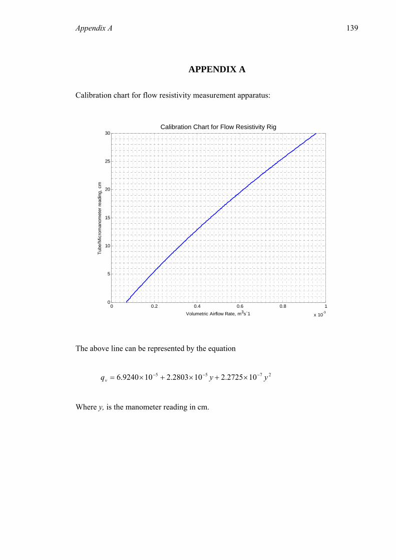
Appendix A 139
APPENDIX A
alibration chart for flow resistivity measurement apparatus: C
0 0.2 0.4 0.6 0.8 1
x 10-3
Calibration Chart for Flow Resistivity Rig30
0
5
10
15
25
20
Volumetric Airflow Rate, m3s-1
Tcr
oman
omet
er re
adin
g, c
m
The above line can be re
e
ube/
Mi
presented by the equation
2755 102725.2102803.2109240.6 yyqv
−−− ×+×+×=
Wher y, is the manometer reading in cm.

Appendix B 140
APPENDIX B Verifying results from large tube w ts and prediction.
[I1,Fs]=LOADIMP('bigA.wmb'); % Loading WINMLS mic1 file into matlab [I2,Fs]=LOADIMP('bigB.wmb'); [I3,Fs]=LOADIMP('bigC.wmb'); [I4,Fs]=LOADIMP('bigD.wmb'); %_PROCESSING RESULTS FROM LARGE IMPEDANCE TUBE_% t = [(1:1:length(I1))/Fs]; % Generate time series N = length(I1); % Length of file in samples w = hanning(N); % Generate hanning window w(1:round(N/2)) = 1; % assign first half of window to unity h1 = I1.*w; % Windowed impulse responses h2 = I2.*w; h3 = I3.*w; h4 = I4.*w; z1 = 0.184; % Position of mic 1 from the sample z2 = 0.368; % Position of mic 2 from the sample z3 = 0.9143; % Position of mic 3 from the sample z4 = 1.2255; % Position of mic 4 from the sample y = [z1 z2 z3 z4]; % Array of mic positions rho = 1.21; % Density of air d = 0.3458; % Tube diameter N1 = length(I1); % Length, in samples, of the input signal Nft = 2^16; % Number of frequency points
= (Fs*(0:((Nft-1)/2))/(Nft-1))'; % Defining frequency axis = 343; % Speed of sound in air
ength = length(f); = max(f)/flength;
spacingA = abs(y(2)-y(1));
acingB = abs(y(3)-y(2)); gC = abs(y(4)-y(1));
fu1A = c/(2*d); % Tube high frequency limit as result of tube diameter fu2A = (0.45*c)/spacingA; % Frequency limit as a result of mic spacing fuA = min(fu1A,fu2A); % Pick the lowest upeer frequency limit flA = 0.05*c/spacingA; % Low frequency limit as a result of mic spacing fu1B = c/(2*d); fu2B = (0.45*c)/spacingB; fuB = min(fu1B,fu2B); flB = 0.05*c/spacingB; fu1C = c/(2*d); fu2C = (0.45*c)/spacingC; fuC = min(fu1C,fu2C);
ith small tube resul
close all clear all
f c k = (2*pi*f)/c; % Wavenumber in air fldf
spspacin

Appendix B 141
flC = 0.05*c/spacingC;
2_fft = fft(h2,(Nft)); 2_fft(1:((Nft)/2)); (h3,(Nft));
h3_fft(1:((Nft)/2));
% Transfer functions
14 = h1freq./h4freq;
12); % Reflection factor ; % Surface impedance % Absorption coefficient
*e 3);
xp(-j*k*spacingC)).*exp(2*j*k*y(2))./(exp(j*k*spacingC)-H14); - RC);
2);
axim ples for eases of plotting
e
% Mic distances from sample % Microphone spacing
% Length in samples of the input signal ;
ound(
(N1D-1))'; % Frequency series
; % Frequency interval in samples
05;
fD(flengthD));
h1_fft = fft(h1,Nft); % Fourier transform of impulse response h1freq = h1_fft(1:((Nft)/2)); % Get rid of negative frequencies hh2freq = h
ffth3_fft = 3freq =h
h4_fft = fft(h4,(Nft)); h4freq = h4_fft(1:((Nft)/2)); H12 = h1freq./h2freq;
13 = h2freq./h3freq; HH
A = (H12-exp(-j*k*spacingA)).*exp(2*j*k*y(2))./(exp(j*k*spacingA)-HRzA = (rho*c)*((RA + 1)./(1 - RA))
alphaA = (1-abs(RA).^2);
c gB)).RB = (H13-exp(-j*k*spa in xp(2*j*k*y(2))./(exp(j*k*spacingB)-H1B = (RB + 1)./(1 - RB);z
alphaB = (1-abs(RB).^2); RC = (H14-ezC = (RC + 1)./(1lphaC = (1-abs(RC).^a
fuAs = fuA/df; % M um and minimum frequency limits in samflAs = flA/df; fuBs = fuB/df; flBs = flB/df; fuCs = fuC/df; flCs = flC/df; %_PROCESSING RESULTS FROM SMALL IMPEDANCE TUBE_% [h1D,FsD]=LOADIMP('smallA.wmb'); [h2D,FsD]=LOADIMP('smallB.wmb'); 1D = 0.1; % Mic possitions of small tubz
z2D = 0.15;
D = [z1D z2D]; yspacingD = yD(2)-yD(1); N1D = length(h1D); = [(1:1:length(h1D))/FsD]t
wD = hanning(N1D); % Generate hanning window unity wD(1:round(N1D/2)) = ones(r N1D/2),1); % Assign first half of window to
imp1D = h1D.*wD; %windowed impulse resopnse
p2D = h2D.*wD; im fD = (FsD*(0:((N1D-1)/2))/k = 2*pi*fD/c; flengthD = length(fD);
fD = max(fD)/flengthDdfu1D = 5.58*c/0.fu2D = 0.45*c/spacingD;
D),fuD = min(min(fu1D,fu2

Appendix B 142
Ds = fuD/dfD;
1D); % FFT of impulse );
N1D)/2));
12D = h1freqD./h2freqD; % Transfer function
spacingD)).*exp(2*j*k*y(2))./(exp(j*k*spacingD)-H12D); )./(1 - RD));
lot(f(flAs:fuAs),alphaA(flAs:fuAs),'r',...
s:fuCs),'g',... Ds:fuDs),'b','LineWidth',2)
label('Frequency (Hz)')
asured in Large and Small Impedance Tubes','FontSize',12)
rid on
D BAZLEY PREDICTION_%
%characteristic impedance of air ; % Flow resisivity of mineral wool
055; % Thickness of sample
% Dimensionless quantity for Delany and Bazley 87*(X.^-0.732)); % Characteristic impedance of mine wool
= (2*pi/c).*f.*(1+0.0978*(X.^-0.700)-j*0.189*(X.^-0.595)); % Complex wavenumber in min wool
t(k*l); % Surface impedance of mineral wool % Reflection factor of mineral wool
ol
gure(1)
'Large Tube Mic positions A and D',...
flD = 0.05*c/spacingD; fuflDs = flD/dfD; h1_fftD = fft(imp1D,Nh1freqD = h1_fftD(1:((N1D)/2) h2_fftD = fft(imp2D,(N1D));h2freqD = h2_fftD(1:(( H RD = (H12D-exp(-j*k*zD = (rho*c)*((RD + 1 alphaD = (1-abs(RD).^2); figure(1) p f(flBs:fuBs), alphaB(flBs:fuBs),'y',... f(flCs:fuCs),alphaC(flC fD(flDs:fuDs),alphaD(flxylabel('Absorption Coefficient') title('Mineral Wool as Meylim([0 1]) ghold on %_DELANY AN Z0 = c*rho; sigma = 25000l = 0.f = fD X = rho*f/sigma; zc = rho*c*(1+0.0571*(X.^-0.754)-j*0.0k z = -j*zc.*coR = (z-Z0)./(z+Z0); alpha = 1-abs(R).^2; % Absorption coefficient of mineral wo fiplot(f,alpha,'k:','LineWidth',2); xlim([15 fuD]) legend('Large Tube Mic positions A and B',... 'Large Tube Mic positions B and C',... 'Small Tube Results',... 'Prediction',4)

Appendix C 143
APPENDIX C
unction with least squares method
lose all;
o = 1.21; % Density of air (kg/m3) peed f sound
= 0.3458/2; % Tube radius (m)
e between tube end and sample = 2 + dL; % Tube length (m)
% Distance from sample to micA 2 = 0.368 + dL; % Distance from sample to micB
43 + dL; % Distance from sample to micC m sample to micD
l'; % File name
DIMP(strcat(char(name(i)),'A.wmb')); % Loading WINMLS mic1 file into matlab LOADIMP(strcat(char(name(i)),'B.wmb'));
OADIMP(strcat(char(name(i)),'C.wmb')); 4,Fs]=LOADIMP(strcat(char(name(i)),'D.wmb'));
_NORMAL TRANSFER FUNCTION TECHNIQUE_%
ngth(I1))/Fs];
ng(N1) % Hanning window (1:N1/2) = 1; % Set first half of window to unity
indow impul
4 = I4.*w;
c = 0.9143; % Position of mic 3 from the sample ; % Position of mic 4 from the sample
ray of mic possitions
ns of mic spacings
% Length, in samples, of the input signal ft = 2^16; % Number of frequency points
(Fs*(0:((Nft-1)/2))/(Nft-1))'; % Defining frequency axis c = 343; % Speed of sound in air k = (2*pi*f)/c; % Wavenumber flength = length(f); df = max(f)/flength; % Frequency interval in samples
omparing standard transfer fC
cclear all; rhc = 343; % S o in air at 23C (m/s) aS = pi*a^2; % Cross-sectional area of the tube (m2) dL = 0; % DistancLz1 = 0.184 + dL; zz3 = 0.91z4 = 1.2255 + dL; % Distance fro x = [z1;z2;z3;z4]; name1 = 'Mineral Woo for i=1:length(name) % Loop if processing more than one file [I1,Fs]=LOA[I2,Fs]=[I3,Fs]=L[I % N1 = length(I1); % Length of impulse in samples t = [(1:1:le % Time series w = hanniwh1 = I1.*w; % W ses h2 = I2.*w; h3 = I3.*w; h za = 0.19; % Position of mic 1 from the sample zb = 0.375; % Position of mic 2 from the sample zzd = 1.2255y = [za zb zc zd]; % Ar spacingA = abs(y(1)-y(2)); % CombinatiospacingB = abs(y(1)-y(3)); spacingC = abs(y(1)-y(4)); N1 = length(h1); Nf =

Appendix C 144
fu1A = c/(2*d); % Fre2A = (0.45*c)/spacingA;
mA = [flA fuA]; % Upper and Lower frequency graph limits
*d); .45*c)/spacingB;
B = min(fu1B,fu2B);
pulse response 1freq = h1_fft(1:((Nft)/2)); % Get rid of negative frequencies
2_fft = fft(h2,(Nft));
13 = h3freq./h1freq;
p(j* )))-(H12.*exp(-j*k*y(1)))); % Reflection
-exp(j* (3)))-(H13.*exp(-j*k*y(1)))); (exp(j*k*y(1)))-exp(j*k*y(4)))./((exp(-j*k*y(4)))-(H14.*exp(-j*k*y(1))));
1)./(1 - RA)); % Surface impedance lphaA = (1-abs(RA).^2); % Absorption coefficient
lphaC = (1-abs(RC).^2);
% Frequency limits in samples
Bs = fuB/df;
lot(f(flAs:fuAs),alphaA(flAs:fuAs),'r','LineWidth',1.5)
s)lot(f(flCs:fuCs),alphaC(flCs:fuCs),'y','LineWidth',1.5)
quency limits of tube fufuA = min(fu1A,fu2A); flA = 0.05*c/spacingA; li fu1B = c/(2fu2B = (0fuflB = 0.05*c/spacingB; limB = [flB fuB]; fu1C = c/(2*d); fu2C = (0.45*c)/spacingC; fuC = min(fu1C,fu2C); flC = 0.05*c/spacingC; limC = [flC fuC]; h1_fft = fft(h1,Nft); % Fourier transform of imh hh2freq = h2_fft(1:((Nft)/2)); h3_fft = fft(h3,(Nft)); h3freq = h3_fft(1:((Nft)/2)); h4_fft = fft(h4,(Nft)); h4freq = h4_fft(1:((Nft)/2)); H12 = h2freq./h1freq; % Transfer function HH14 = h4freq./h1freq; RA = (H12.*(exp(j*k*y(1)))-ex k*y(2)))./((exp(-j*k*y(2factor RB = (H13.*(exp(j*k*y(1))) k*y(3)))./((exp(-j*k*yRC = (H14.* zA = (rho*c)*((RA +a zB = (rho*c)*((RB + 1)./(1 - RB)); alphaB = (1-abs(RB).^2); zC = (rho*c)*((RC + 1)./(1 - RC)); a fuAs = fuA/df; flAs = flA/df; fuflBs = flB/df; fuCs = fuC/df; flCs = flC/df; figure(1) phold on plot(f(flBs:fuBs),alphaB(flBs:fuB ,'k','LineWidth',1.5) p
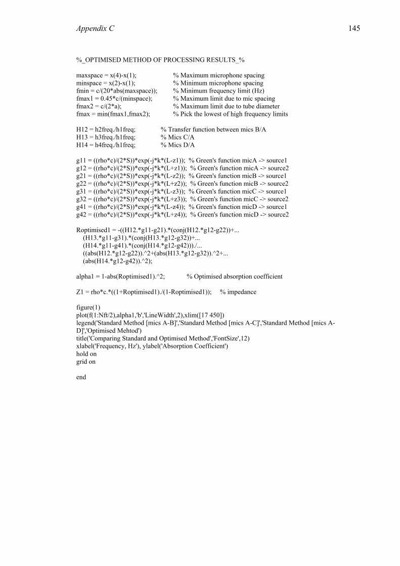
Appendix C 145
SING RESULTS_%
% Maximum microphone spacing
in = c/(20*abs(maxspace)); % Minimum frequency limit (Hz) minspace); % Maximum limit due to mic spacing
% Maximum limit due to tube diameter 2); % Pick the lowest of high frequency limits
q; % Transfer function between mics B/A 13 = h3freq./h1freq; % Mics C/A
freq; % Mics D/A
(-j*k*(L-z1)); % Green's function micA -> source1 (-j*k*(L+z1)); % Green's function micA -> source2
))*exp(-j*k*(L-z2)); % Green's function micB -> source1 22 = ((rho*c)/(2*S))*exp(-j*k*(L+z2)); % Green's function micB -> source2
- source2
41 = ((rho*c)/(2*S))*exp(-j*k*(L-z4)); % Green's function micD -> source1 exp(-j*k*(L+z4)); % Green's function micD -> source2
optimised1 = -((H12.*g11-g21).*(conj(H12.*g12-g22))+... nj(H13.*g12-g32))+...
4.*g12-g42)))./... ((abs(H12.*g12-g22)).^2+(abs(H13.*g12-g32)).^2+...
).^2);
lpha1 = 1-abs(Roptimised1).^2; % Optimised absorption coefficient
ised1)./(1-Roptimised1)); % impedance
gure(1)
Standard Method [mics A-B]','Standard Method [mics A-C]','Standard Method [mics A-
label('Frequency, Hz'), ylabel('Absorption Coefficient')
%_OPTIMISED METHOD OF PROCES maxspace = x(4)-x(1); minspace = x(2)-x(1); % Minimum microphone spacing fmfmax1 = 0.45*c/(fmax2 = c/(2*a); fmax = min(fmax1,fmax H12 = h2freq./h1freHH14 = h4freq./h1 g11 = ((rho*c)/(2*S))*expg12 = ((rho*c)/(2*S))*expg21 = ((rho*c)/(2*Sgg31 = ((rho*c)/(2*S))*exp(-j*k*(L z3)); % Green's function micC -> source1g32 = ((rho*c)/(2*S))*exp(-j*k*(L+z3)); % Green's function micC -> gg42 = ((rho*c)/(2*S))* R (H13.*g11-g31).*(co (H14.*g11-g41).*(conj(H1 (abs(H14.*g12-g42) a Z1 = rho*c.*((1+Roptim fiplot(f(1:Nft/2),alpha1,'b','LineWidth',2),xlim([17 450]) legend('D]','Optimised Mehtod') title('Comparing Standard and Optimised Method','FontSize',12) xhold on grid on end

Appendix D 146
APPENDIX D Comparing the original least squares technique with the extended version.
o = 1.21; % Density of air (kg/m3)
) of the tube (m2)
L = 0; % Distance between tube end and sample
ame1 = 'Mineral Wool';
')); % Loading WINMLS mic1 file into matlab
r(name(i)),'C.wmb')); 4,Fs]=LOADIMP(strcat(char(name(i)),'D.wmb'));
1 = length(I1);
an(1:N1/2) = 1; an;
om the sample 5; % Position of mic 2 from the sample 43; % Position of mic 3 from the sample
d = 1.2255; % Position of mic 4 from the sample za zb zc zd]; % Array of mic positions
spacingA = abs(y(1)-y(2)); spacingB = abs(y(1)-y(3)); spacingC = abs(y(1)-y(4)); spacingD = abs(y(2)-y(3)); spacingE = abs(y(2)-y(4)); spacingF = abs(y(3)-y(4)); rho=1.21; d = 0.3458; %Tube diameter N1 = length(h1); % Length, in samples, of the input signal Nft = 2^16; % Number of frequency points f = (Fs*(0:((Nft-1)/2))/(Nft-1))'; % Defining frequency axis k = (2*pi*f)/c;
close all; clear all; rhc = 343; % Speed of sound in air at 23C (m/s) a = 0.3458/2; % Tube radius (mS = pi*a^2; % Cross-sectional area dL = 2 + dL; % Tube length (m) z1 = 0.184 + dL; % Distance from sample to micA z2 = 0.368 + dL; % Distance from sample to micB z3 = 0.9143 + dL; % Distance from sample to micC z4 = 1.2255 + dL; % Distance from sample to micD x = [z1;z2;z3;z4]; n for i=1:length(name) [I1,Fs]=LOADIMP(strcat(char(name(i)),'A.wmb[I2,Fs]=LOADIMP(strcat(char(name(i)),'B.wmb')); [I3,Fs]=LOADIMP(strcat(cha[I Nhan = hanning(N1) hh1 = I1.*hh2 = I2.*han; h3 = I3.*han; h4 = I4.*han; za = 0.19; % Position of mic 1 frzb = 0.37zc = 0.91zy = [

Appendix D 147
flength = length(f); f = max(f)/flength;
ame2 = strcat(name(i),'B.wmb'); ame3 = strcat(name(i),'C.wmb');
strcat(name(i),'D.wmb');
= x(4)-x(1); % Maximum microphone spacing ophone spacing
(Hz) m limit due to mic spacing
iameter cy limits
e response for micA
% Number of sample points = hanning(N); % Generate hanning window
% Assign first half of window to unity
% Pick the first N points of yA
wA = yA.*w; % Apply hanning window to micA impulse reponse % MicB
% MicC % MicD
(ywA))/Fs]; % Generate time series (s) 1)))/(N-1))'; % Generate frequency series (Hz) /2))/c; % Wave number array
e responses
1 = (YA(1:N/2)); % Pick the first N/2 points of Y1 % Y2
% Y3 % Y4
% Transfer function between mics B/A % Mics C/A
14 = Y4./Y1; % Mics D/A % Mics C/B % Mics D/B
Y3; % Mics D/C
ce1 L+ ource2
- micB -> source1 *S))*exp(-j*k*(L+z2)); % Green's function micB -> source2
31 = ((rho*c)/(2*S))*exp(-j*k*(L-z3)); % Green's function micC -> source1
d fname1 = strcat(name(i),'A.wmb'); fnfnfname4 =
axspacemminspace = x(2)-x(1); % Minimum micrfmin = c/(20*abs(maxspace)); % Minimum frequency limit fmax1= 0.45*c/(minspace); % Maximufmax2= c/(2*a); % Maximum limit due to tube dfmax = min(fmax1,fmax2); % Pick the lowest of high frequen [yA, Fs] = loadimp(char(fname1)); % Load WinMLS impuls[yB, Fs] = loadimp(char(fname2)); % MicB [yC, Fs] = loadimp(char(fname3)); % MicC [yD, Fs] = loadimp(char(fname4)); % MicD N = length(yA); ww(1:N/2) = ones(N/2,1); yA = (yA(1:N)); yB = (yB(1:N)); % yB yC = (yC(1:N)); % yC yD = (yD(1:N)); % yD yywB = yB.*w; ywC = yC.*w; ywD = yD.*w; t = [(1:1:lengthf = (Fs*(0:((N-k=(2*pi*f(1:N YA = fft(ywA); % Fourier Transform on mic A impulsYB = fft(ywB); % Mic B YC = fft(ywC); % Mic C YD = fft(ywD); % Mic D YY2 = (YB(1:N/2)); Y3 = (YC(1:N/2)); Y4 = (YD(1:N/2)); H12 = Y2./Y1; H13 = Y3./Y1; HH23 = Y3./Y2;
24 = Y4./Y2; HH34 = Y4./ g11 = ((rho*c)/(2*S))*exp(-j*k*(L-z1)); % Green's function micA -> sourg12 = ((rho*c)/(2*S))*exp(-j*k*( z1)); % Green's function micA -> sg21 = ((rho*c)/(2*S))*exp(-j*k*(L z2)); % Green's functiong22 = ((rho*c)/(2g

Appendix D 148
xp(-j*k*(L+z3)); % Green's function micC -> source2 *exp(-j*k*(L-z4)); % Green's function micD -> source1
42 = ((rho*c)/(2*S))*exp(-j*k*(L+z4)); % Green's function micD -> source2
conj(H12.*g12-g22))+... % Original optimised method -g32))+... -g42)))./...
((abs(H12.*g12-g22)).^2+(abs(H13.*g12-g32)).^2+...
d optimised method
.*g1
(H24.*g21-g41).*(conj(H24.*g22-g42))+...
32)).^2+... 2)).^2+... 2)).^2);
2; on coefficient original 2; n coefficient extended
1 = rho*c.*((1+Roptimised1)./(1-Roptimised1)); % Surface impedance original edance extended
fficilot(f(1:N/2),alpha1,'b',f(1:N/2),alpha2,'r','LineWidth',2),xlim([17 450])
Exte ised Methods','FontSize',12) 'Abs efficient')
old on
g32 = ((rho*c)/(2*S))*eg41 = ((rho*c)/(2*S))g Roptimised1 = -((H12.*g11-g21).*( (H13.*g11-g31).*(conj(H13.*g12 (H14.*g11-g41).*(conj(H14.*g12 (abs(H14.*g12-g42)).^2); Roptimised2 = -((H12.*g11-g21).*(conj(H12.*g12-g22))+... % Extende (H13.*g11-g31).*(conj(H13.*g12-g32))+... (H14.*g11-g41).*(conj(H14 2-g42))+... (H23.*g21-g31).*(conj(H23.*g22-g32))+... (H34.*g31-g41).*(conj(H34.*g32-g42)))./... ((abs(H12.*g12-g22)).^2+(abs(H13.*g12-g (abs(H14.*g12-g42)).^2+(abs(H23.*g22-g3 (abs(H24.*g22-g42)).^2+(abs(H34.*g32-g4 alpha1 = 1-abs(Roptimised1).^ % Absorptialpha2 = 1-abs(Roptimised2).^ % Absorptio ZZ2 = rho*c.*((1+Roptimised2)./(1-Roptimised2)); % Surface imp figure(1) set(gcf,'Name','Absorption Coe ent') plegend('Original Optimisation Method','Extended Optimisation Method') grid on title('Comparing Standard and nded Optimxlabel('Frequency, Hz'), ylabel( orption Coh end

Appendix E 149
APPENDIX E
MATLAB script for processing results from accelerometer data in section 4.3
%____ Processing Accelerometer Measurements ____% lose all; c
clear all; c = 343; % Speed of sound in air
ncy uency
of colours for plot
r i = 1:length(s)
mber of sample points
dow to mic A impulse response
t = [(1:1:length(ywA))/Fs]; % Generate time series (s) (Fs*(0:((N-1)))/(N-1))'; % Generate frequency series (Hz)
k=(2*pi*f(1:N/2))/c; % Wave number array
YA = fft(ywA); % Fourier Transform on impulse responses YA = 20*log(abs(YA)); % Log of FFT plot(f,YA,str(i,:),'LineWidth',2) hold on grid on legend('With Surround','Without Surround',4) xlabel('Frequency, Hz') ylabel('Level, dB') title('Acceleration Level versus Frequency For Different Mounting Conditions','FontSize',13) xlim([fmin fmax]) end
fmax = 200; % max frequefmin = 30; % min freq str(1,1:2) = 'r-'; % String to define order str(2,1:2) = 'b-'; 1 = 'acc surround'; % Input file names s
s2 = 'acc no surround'; fo files = s(i); % Pick successive files to process fname = strcat(files,'.wmb'); % Add on suffix to complete file name
[yA, Fs] = loadimp(char(fname)); % Load winMLS files N = length(yA); % Nu w = hanning(N); % Generate Hanning window w(1:N/2) = 1; % Assign first half of window to unity yA = (yA(1:N)); % Pick the first N points ywA = yA.*w; % Apply Hanning win f =

Appendix F 150
APPENDIX F
A: Surround mounted membrane on La B: Clamped memrge brane on large sample holder
sample holder
C: Impedance tube mounting rings
ith the sample in place between the mounting rings, was jacked
ating a
ped condition.
The sample holder, w
into place to provide a termination at the impedance tube walls approxim
clam

Appendix G 151
APPENDIX G Analogue circuit analysis of absorber with and without surround.
close all; clear all; c = 343; % Speed of sound in air rho = 1.21; % Density of air Z0 = c*rho; % Characteristic impedance of air f = 1:1:400; % Frequency spectrum, Hz w = 2*pi*f; % Angular frequency k = w/c; % Wavenumber in air V = 0.035; % Volume of backing a = 0.135; % Radius of plate with surround plus 1/3 of surround SD = pi*(a^2); % Area of plate and surround sigma = 10200; % Flow resistivity of absorbent X = rho*f/sigma; Z2 = rho*c*(1+0.0571*(X.^-0.754)-j*0.087*(X.^-0.732)); k2 = (2*pi/c).*f.*(1+0.0978*(X.^-0.700)-j*0.189*(X.^-0.595)); d2 = 0.15; zs2 = -j*rho*c.*cot(k2*d2); % Delany and Bazley prediction for porous absorbent in cabi et
%
SUR = 0.03402; % Mass of moving surround MMEM = 0.1077; % Mass of moving hardboard MMS = MSUR+MMEM; % Combined mass of surround and plate (hardboard),kg RAF1 = (rho*c.*(k.^2))./(2*pi); % Radiation resistance MAF1 = j*w.*((8*rho)/(3*(pi^2)*a)); % Radiation mass BL = 15; RES = 360.575; RMS = (BL^2)/RES; RAD = RMS/(SD^2); % Approximate resistive losses in diaphragm based on L/S data RAB = zs2; % Resistive losses in cabinet CMS = 205.5E-6; % Compliance of surround/plate in mechanical units CAD = CMS*(SD^2); % Diaph compliance in acoustic units CAB = V/(rho*(c^2)); % Comp ance of cabinet in acoustic units
(1./(j.*w.*((CAD*CAB)/(CAD+CAB)))); % Total compliance in acoustic units AT = RAD+RAB+RAF1; % Total resistive damping in acoustical units
% Complex reflection factor of system alpha = 1-R.*conj(R); % Absorption coefficient figure(1) plot(f,alpha,'b','LineWidth',2) hold on %_ Without Surround _% a = 0.14;
n %_ With Surround _ M
ragmli
CAT = RMAD = (j.*w.*((MMS/(SD^2)))) + MAF1; % Total mass impedance acoustic units ZAF = Z0/SD; Z = SD*(RAT + MAD + CAT + ZAF); % Total surface impedance of system R = (Z-Z0)./(Z+Z0);

Appendix G 152
SD = pi*(a^2); MEM2 = 0.173;
ardboard),kg
ES = 360.575; 2)/RES;
S/(SD^2); % Resistive losses in diaphragm 2; % Resistive losses in cabinet
/(E*( plate in mechanical units ce in acoustic units
s
ping in acoustical units AD = (j.*w.*(MMS/(SD^2)))+MAF1; % Total mass impedance acoustic units
AD + CAT + ZAF); % Total surface impedance of system
.*conj(R); % Absorption coefficient
gure(1) th',2)
tle('Equivalent Circuit Model of Membrane Absorber With and Without Surround
MMMS = MMEM2/5; % Combined mass of surround and plate (h RRMS = (BL^RAD = RMRAB = zs E = 0.1e6; % Youngs Modulus mu = 0.7; % Poisson Ratio h = 3.2e-3; % Thickness of plate CMS = 180*(1-(mu^2))*(a^2) h^3)); % Compliance of surround/CAD = CMS*(SD^2); % Diaphragm complianCAB = V/(rho*(c^2)); % Comliance of cabinet in acoustic unit CAT = 1./(j.*w.*((CAD*CAB)/(CAD+CAB))); % Total compliance in acoustic units RAT = RAD+RAB+RAF1; % Total resistive damMZAF = Z0/SD; Z = SD*(RAT + M R = (Z-Z0)./(Z+Z0); % Complex reflection factor of systemalpha = 1-R fiplot(f,alpha,'r','LineWidtiMounting','FontSize',13) legend('With Surround','Without Surround') xlabel('Frequency, Hz'),ylabel('Absorption Coefficient') ylim([0 1.1]) grid on

Appendix H 153
APPENDIX H
odels for
l rubber membranes.
ensi
-
'No Surround Min Wool'; rdboard';
s for plotting
-';
for i = 1:length(name) fname1 = strcat(name(i),'A.wmb'); fname2 = strcat(name(i),'B.wmb'); fname3 = strcat(name(i),'C.wmb'); fname4 = strcat(name(i),'D.wmb'); maxspace = x(4)-x(1); % Maximum microphone spacing minspace = x(2)-x(1); % Minimum microphone spacing fmin = c/(20*abs(maxspace)); % Minimum frequency limit (Hz) fmax1= 0.45*c/(minspace); % Maximum limit due to mic spacing fmax2= c/(2*a); % Maximum limit due to tube diameter fmax = min(fmax1,fmax2); % Pick the lowest of high frequency limits [yA, Fs] = loadimp(char(fname1)); % Load WinMLS impulse response for micA [yB, Fs] = loadimp(char(fname2)); % MicB [yC, Fs] = loadimp(char(fname3)); % MicC [yD, Fs] = loadimp(char(fname4)); % MicD N = length(yA); % Number of sample points w = hanning(N); % Generate Hanning window w(1:N/2) = ones(N/2,1); % Assign first half of window to unity yA = (yA(1:N)); % Pick the first N points of yA yB = (yB(1:N)); % yB yC = (yC(1:N)); % yC yD = (yD(1:N)); % yD
ATLAB script for comparing impedance tube results with transfer matrix mM
hardboard and viny
close all; clear all; rho = 1.21; % D ty of air (kg/m3) c = 343; % Speed of sound in air at 23C (m/s) Z0 = rho*c; % Characteristic impedance of air a = 0.3458; % Tube radius (m)
= pi*a^2; % Cross sectional area of the tube (m2) SdL = 0; % Distance between tube end and sample
(mL = 2 + dL; % Tube length ) z1 = 0.184 + dL; % Distance from sample to micA
; % Distance from sample to micB z2 = 0.368 + dLz3 = 0.9143 + dL; % Distance from sample to micC 4 = 1.2255 + dL; % Distance from sample to micD z
x = [z1;z2;z3;z4];
ame1 = 'With Surround Min Wool'; % File names nname2 =name3 = 'With Surround Haname4 = 'No Surround Hardboard'; str(1,1:2) = 'r-'; % String of colourstr(2,1:2) = 'b-';
; str(3,1:2) = 'r-') = 'bstr(4,1:2

Appendix H 154
ywA = yA.*w; % Ap micA impulse response wB = yB.*w; % Mi
requency series (Hz) = (2*pi*f(1:N/2))/c; % Wave number array
wA); % Fourier Transform on mic A impulse responses wB); % Mic B
of YA
en mics B/A
% Mics D/B
% Green's function micA -> source1 % Green's function micA -> source2 % Green's function micB -> source1
tion micB -> source2 tion micC -> source1
*S))*exp(-j*k*(L+z3)); % Green's function micC -> source2 *S))*exp(-j*k*(L-z4)); % Green's function micD -> source1 *S))*exp(-j*k*(L+z4)); % Green's function micD -> source2
(H12.*g12-g22))+...% Optimised reflection factor from impedance
32))+... 42))+... 32))+...
g22g3
nce tube measurements ised)); easurements
ineW
ineW
nd
ply Hanning window tocB y
ywC = yC.*w; % MicC ywD = yD.*w; % MicD f = (Fs*(0:((N-1)))/(N-1))'; % Generate fk YA = fft(yYB = fft(yYC = fft(ywC); % Mic C YD = fft(ywD); % Mic D Y1 = (YA(1:N/2)); % Pick the first N/2 points Y2 = (YB(1:N/2)); % YB Y3 = (YC(1:N/2)); % YC Y4 = (YD(1:N/2)); % YD H12 = Y2./Y1; % Transfer function betweH13 = Y3./Y1; % Mics C/A H14 = Y4./Y1; % Mics D/A H23 = Y3./Y2; % Mics C/B H24 = Y4./Y2; H34 = Y4./Y3; % Mics D/C g11 = ((rho*c)/(2*S))*exp(-j*k*(L-z1));g12 = ((rho*c)/(2*S))*exp(-j*k*(L+z1));g21 = ((rho*c)/(2*S))*exp(-j*k*(L-z2));g22 = ((rho*c)/(2*S))*exp(-j*k*(L+z2)); % Green's funcg31 = ((rho*c)/(2*S))*exp(-j*k*(L-z3)); % Green's funcg32 = ((rho*c)/(2g41 = ((rho*c)/(2g42 = ((rho*c)/(2 Roptimised = -((H12.*g11-g21).*(conjtube measurments (H13.*g11-g31).*(conj(H13.*g12-g (H14.*g11-g41).*(conj(H14.*g12-g (H23.*g21-g31).*(conj(H23.*g22-g (H24.*g21-g41).*(conj(H24.* -g42))+... (H34.*g31-g41).*(conj(H34.* 2-g42)))./... ((abs(H12.*g12-g22)).^2+(abs 13.*g12-g32)).^2+... (H (abs(H14.*g12-g42)).^2+(abs(H23.*g22-g32)).^2+... (abs(H24.*g22-g42)).^2+(abs(H34.*g32-g42)).^2); alpha = 1-abs(Roptimised).^2; % Absorption coefficient from impedaZ = Z0.*((1+Roptimised)./(1-Roptim % Surface impedance from impedance tube m figure(1) if i<=2 subplot(2,1,1) plot(f(1:N/2),alpha,str(i,:),'L idth',2) hold on else figure(1) subplot(2,1,2) plot(f(1:N/2),alpha,str(i,:),'L idth',2) hold on end e

Appendix H 155
epth ent 1 = 0.15; % Air gap depth
us (vinyl) us embrane (hardboard)
= (1:1:300)'; % Array of frequencies nguesist due to mounting of the membrane ave
igma = 10200; % Flow resistivity of absorbent itle prediction
)-j* X.^-0.732)); .^-0 0.189*(X.^-0.595));
s2 = -j*Z2.*cot(k2*d2); .
%Final surface impedance of vinyl rubber %Final surface impedance of hardboard
% Reflection factor for vinyl rubber lphaV = 1-(abs(RV).^2); % Absorption coefficient for vinyl rubber
oard hardboard
label('Frequency, Hz'),ylabel('absorption coefficient')
nd','Without Surround','Transfer Matrix Model')
icient')
x Model')
rid on
%_ TRANSFER MATRIX MODEL _% d2 = 0.15; % D of absorbdmV = 2.81; % Aco tic mass per unit area of membranemH = 2.57; % Aco tic mass per unit area of mf w = 2*pi.*f; % A lar frequency rm = 10; % R ive losses k1 = w/c; % W number sX = rho*f/sigma; % Un ss quantity for Delany and Bazley Z2 = Z0*(1+0.0571*(X.^-0.754 0.087*(k2 = (2*pi/c).*f.*(1+0.0978*(X .700)-j* zzs3 = (-j*zs2.*Z0.*cot(k1*d1)+Z0 ^2 )./ (zs2 -j*Z0.*cot(k1*d1)); zs4V = zs3 + j*w*mV +rm; zs4H = zs3 + j*w*mH +rm; RV = (zs4V - Z0)./(zs4V + Z0); a RH = (zs4H - Z0)./(zs4H + Z0); % Reflection factor for hardbalphaH = 1-(abs(RH).^2); % Absorption coefficient for figure(1) set(gcf,'Name','Absorption Coefficient') subplot(2,1,1) plot(f,alphaV,'g','LineWidth',2) xtitle('Vinyl Rubber') legend('With Surrouaxis([20 150 0 1]) grid on subplot(2,1,2) plot(f,alphaH,'g','LineWidth',2) xlabel('Frequency, Hz'),ylabel('absorption coefftitle('Hardboard') legend('With Surround','Without Surround','Transfer Matriaxis([20 150 0 1]) g

Appendix I 156
APPENDIX I
lent re:
bols rm :
refers to the quantity, i.e. Mass (M), Resistance (R), Compliance (C), Impedance
of quantity i.e. Electrical (E), Mechanical (M) or
the valu
S, refers to the diaphragm with an air load
total
mponent
he total acoustic compliance is written as
ass of the diaphragm with an air load is written as,
en as,
Rules for equiva circuit nomenclatu
xyzAIn general the sym are written in the fo
A
(Z)… etc
x refers to the units or type
Acoustic (A)
y refers to other information regarding e e.g.
Subscript: B, refers to the back of the diaphragm (the cabinet)
D, refers to the diaphragm without an air load
T, refers to a
V, refers to a variable co
: ABCFor example: T
The mechanical m
MSM
ATR The total damping in acoustic units is writt

Appendix J 157
APPENDIX J
Comparing impedance tube results with lumped parameter predictions
o = 1.21; % Density of air (kg/m3) = 344= 0.3
S = pi* % Cross-sectional area of the tube (m2) dL = 0; % Distance between tube end and sample
= 2 + dL; % Tube length (m) 0.184 +
= 0.3z3 = 0.9 % Distance from sample to micC z4 = 1.2 % Distance from sample to micD
= [z1;z2;z3;z4];
es(1 it case ='Op
microphone spacing microphone spacing
z) ax1= 0.45*c/(minspace); % Maximum limit due to mic spacing ax2= c/(2*a); % Maximum limit due to tube diameter
lim ts
[yA, Fs] = loadim[yB, Fs] = loadim[yC, Fs] = loadimp(char name3)); % MicC [yD, Fs] = loadimp(char name4)); % MicD
= leng A); hanning(N); % Generate hanning window
(1:N/2) = 1; % Assign first half of window to unity
= (yA(1:N)); % Pick the first N points of yA % yB % yC % yD
ywA = yA.*w; % Apply hanning window to micA impulse reponse ywB = yB.*w; % MicB ywC = yC.*w; % MicC ywD = yD.*w; % MicD t = [(1:1:length(ywA))/Fs]; % Generate time series (s) f = (Fs*(0:((N-1)))/(N-1))'; % Generate frequency series (Hz) k=(2*pi.*f(1:N/2))./c; % Wave number array
close all; clear all; rhc ; % Speed of sound in air at 23C (m/s) a 458; % Tube diameter (m)
(a/2)^2;
Lz1 = dL; % Distance from sample to micA z2 68 + dL; % Distance from sample to micB
143 + dL; 255 + dL;
x valu ) = 1e6; % Approximation to resistance of open circufiles1 en Circuit'; for i = 1:length(files) fname1 = strcat(files(i),'A.wmb'); fname2 = strcat(files(i),'B.wmb'); fname3 = strcat(files(i),'C.wmb'); fname4 = strcat(files(i),'D.wmb'); maxspace = x(4)-x(1); % Maximum minspace = x(2)-x(1); % Minimum fmin = c/(20*abs(maxspace)); % Minimum frequency limit (Hfmfmfmax = min(fmax1,fmax2); % Pick the lowest of high frequency i
p(char(fname1)); % Load WinMLS impulse response for micA p(char(fname2)); % MicB
(f(f
N th(y % Number of sample points w = w yAyB = (yB(1:N)); yC = (yC(1:N)); yD = (yD(1:N));
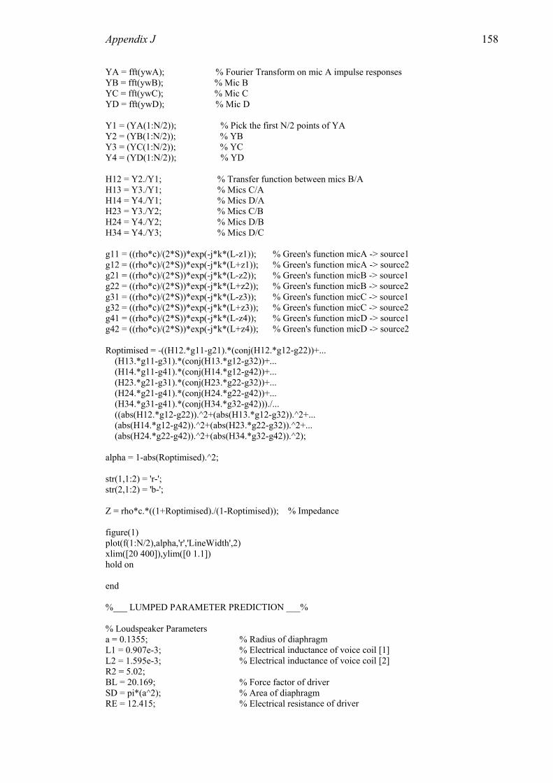
Appendix J 158
YA = fft(ywA); % Fourier Tr ponses B = fft(ywB); % Mic B C = fft(ywC); % Mic C
1 = (YA(1:N/2)); % Pick the first N/2 points of YA (1:N/2)); % YB (1:N/2)); % YC (1:N/2)); % YD
B/A
on micA -> source1 on micA -> source2 on micB -> source1
))*exp(-j*k*(L+z2)); % Green's function micB -> source2 *exp e1
e2 (-j*k*(L-z4)); % Green's function micD -> source1
xp(-j*k*(L+z4)); % Green's function micD -> source2
j(H12.*g12-g22))+... 2))+... 2))+... 2))+...
g2g3
% Impedance
DICTION ___%
adius of diaphragm lectrical inductance of voice coil [1] lectrical inductance of voice coil [2]
e of driver
ansform on mic A impulse resYYYD = fft(ywD); % Mic D YY2 = (YBY3 = (YC
4 = (YDY
H12 = Y2./Y1; % Transfer function between mics H13 = Y3./Y1; % Mics C/A
H14 = Y4./Y1; % Mics D/A H23 = Y3./Y2; % Mics C/B
H24 = Y4./Y2; % Mics D/B H34 = Y4./Y3; % Mics D/C g11 = ((rho*c)/(2*S))*exp(-j*k*(L-z1)); % Green's functig12 = ((rho*c)/(2*S))*exp(-j*k*(L+z1)); % Green's functi
S))*exp(-j*k*(L-z2)); % Green's functig21 = ((rho*c)/(2*22 = ((rho*c)/(2*Sg
g31 = ((rho*c)/(2*S)) (-j*k*(L-z3)); % Green's function micC -> sourc(-j*k*(L+z3)); % Green's function micC -> sourcg32 = ((rho*c)/(2*S))*exp
41 = ((rho*c)/(2*S))*expgg42 = ((rho*c)/(2*S))*e
nRoptimised = -((H12.*g11-g21).*(co (H13.*g11-g31).*(conj(H13.*g12-g3 (H14.*g11-g41).*(conj(H14.*g12-g4 (H23.*g21-g31).*(conj(H23.*g22-g3
(H24.*g21-g41).*(conj(H24.* 2-g42))+... * (H34.*g31-g41).*(conj(H34. 2-g42)))./...
((abs(H12.*g12-g22)).^2+(abs(H13.*g12-g32)).^2+... (abs(H14.*g12-g42)).^2+(abs(H23.*g22-g32)).^2+...
bs(H3 (abs(H24.*g22-g42)).^2+(a 4.*g32-g42)).^2); lpha = 1-abs(Roptimised).^2; a
str(1,1:2) = 'r-'; str(2,1:2) = 'b-';
= rho*c.*((1+Roptimised)./(1-Roptimised));Z figure(1) plot(f(1:N/2),alpha,'r','LineWidth',2)
lim([20 400]),ylim([0 1.1]) xhold on end
___ LUMPED PARAMETER PRE% % Loudspeaker Parameters a = 0.1355; % RL1 = 0.907e-3; % E
2 = 1.595e-3; % ELR2 = 5.02; BL = 20.169; % Force factor of driver
SD = pi*(a^2); % Area of diaphragmE = 12.415; % Electrical resistancR

Appendix J 159
amping of diaphragm in electrical units echanical compliance of driver with air load
= 20:1000;
Width of cabinet/sample holder Height of cabinet/sample holder
= 0.226; % Depth of cabinet/sample holder r
pedance of air
anical damping/resistance of diaphragm with airload tance/damping of diaphragm in acoustic units
n in cabinet
*.
AD = CMS*(SD^2); % Compliance of diaphragm in acoustic units c units of cabinet
resistance values
istance values e due to electrical inductance in acoustic units
nce due to electrical resistance in acoustic units z3 = (BL^2)/(REV*(SD^2)); % Impedance due to variable resistance in acoustic units
(1./(j.*w.*(((SD^2).*L2)./(BL^2)))); ZEA = 1./((1./z1)+(1./z2)+(1./z3)+(1./z4)); % Combined impedance due to electronic
coustic units .*((CAD*CAB)/(CAD+CAB)))); % Combined acoustic compliance of entire system
RAT = RAD+RAB; % Comined acoustic damping of entire system ance of a baffled piston
MAT = (j.*w.*(MMS/(SD^2)))-MAF1; % Combined mass loading of entire system (minus air load as measured in free field)
T + ZAF); % Specific acoustic impedance of entire system
1-R.*conj(R);
(1) lot(f,alpha,'b','LineWidth',1.5)
tle('Using a Loudspeaker as an Absorber', 'FontSize',13) nce Tube', 'Equivalent Circuit Prediction')
MMS = 28.152e-3; % Moving mass of diaphragm (with air load)RES = 360.575; % DCMS = 385.276e-6; % MLE=L1; f w = 2*pi*f; k = w./c; x = 0.38; %y = 0.505; % dV = x*y*d; % Volume of cabinet/sample holdeZ0 = c*rho; % Characteristic im RMS = (BL^2)/RES; % MechRAD = RMS/(SD^2); % ResisRAF = 0; sigma = 10200; % Flow resistivity of absorbent X = rho*f/sigma; % Dela y and Bazley prediction for absorbent Z0 = rho*c; d2 = 0.3; Z2 = rho*c*(1+0.0571*(X.^-0.754)-j*0.087 (X.^-0.732)); k2 = k.*(1+0.0978*(X.^-0.700)-j*0.189*(X ^-0.595)); RAB = -j*rho*c.*cot(k2*d2); CCAB = V/(rho*(c^2)); % Compliance in acoustiZAF = Z0/SD; val = values'; % Array offor i = 1:length(val) REV = val(i); % Variable res z1 = 1./(j*w*(((SD^2)*LE)/(BL^2))); % Impedanc z2 = (BL^2)/(RE*(SD^2)); % Impeda z4 = ((BL^2)/(R2*(SD^2)))+ components in a CAT = (1./(j*w MAF1 = j*w.*((8*rho)/(3*(pi^2)*a)); % Radiation imped as MMS w Z = SD*(ZEA + RAT + MAT + CA R = (Z-Z0)./(Z+Z0); alpha = figurepxlabel('Frequency, Hz'),ylabel('Absorption Coefficient') tilegend('Results from Impedagrid on end

Appendix K 160
APPENDIX K
Comparing impedance tube measurements with predictions from the equivalent circuit
ach load resistance connected to terminals. model for e
Closed Circuit 1 Ohms
100 200 300 4000
0.5
1
. , Hz Freq
α
100 200 300 4000
0.5
1 1
. , Hz
α 0.5
0100 200 300 400
Freq. Freq, Hz
α
5 Ohms
100 200 300 4000
0.5
1
. , Hz Freq
s10 Ohm 50 Ohms
α
100 200 300 4000
0.5
1 1
0.5
. Freq, Hz
α
0100 200 300 400
. Freq, Hzα
100 Ohms
Open Circuit
100 200 300 400
1
0
0.5
Measured DataPredictionsα
. Freq, Hz

Appendix L 161
APPENDIX L
100 200 300 4000
0.2
0.4
0.6
0.8
1 Ω 5 Ω 10 ΩPredicted Absorption Curves, Varying Load Capacitance and Resistance in Parallel
1
Freq, Hz
α
100 200 300 4000
0.2
0.4
0.6
0.8
1
Freq, Hzα
1
0.8
0.6
0.4
0.2
0100 200 300 400
Freq, Hz
α100 200 300 400
0
0.2
0.4
0.6
0.8
1
Freq, Hz
α
50 Ω
1 μF 10 μF 22 μF 47 μF100 μF220 μF470 μF
100 200 300 4000
0.2
0.4
0.6
0.8
1
Freq, Hz
α100 Ω
100 200 300
1
0.8
0.6
0.4
0.2
4000
Freq, Hz
α
500 Ω

Bibliography 172
B
F. Alton Everest, Master Handbook of Acoustics, 4th edn., McGraw-Hill, (2001). M. Barron, Auditorium Acoustics and Architectural Design, E and F. N. Spon (1993). L. L. Beranek, Acoustics, Acoustical Society of America, (1996). J. Borwick, Loudspeaker and Headphone handbook, 2nd edn, Focal Press, (1994). J. Borwick, Loudspeaker and Headphone handbook, 3rd edn, Focal Press (2001). M. Colloms, High Performance Loudspeakers, 6th edn, John Wiley and sons (2005). T. J. Cox and P. D’Antonio, Acoustic absorbers and diffusers, Spon Press (2004). F. Fahy, Foundations of Engineering Acoustics, Academic Press, (2001) F. A. Fischer, Fundamentals of Electroacoustics, Interscience Publishers, inc., New York, (1955). L.E. Kinsler, A. R. Frey, A. B. Copens and J. V. Sanders, Fundamentals of Acoustics, 3rd edn, John Wiley and Sons (1982).
. Kuttruff , Room Acoustics, 4th edn., Spon press (2000). F. P. Mechel, Formulas of Acoustics, Springer, (2002). P. M. Morse and K. U. Ingard, Theoretical Acoustics, McGraw-Hill, (1968). M. Rossi, Acoustics and Electroacoustics, Artech House, (1988). I. R. Sinclair (ed), Audio and Hi-Fi Handbook, 2nd edn, Butterworth-Heinemann, (1993). M. C. M. Wright (ed), Lecture Notes on the Mathematics of Acoustics, Imperial College Press, (2005).
IBLIOGRAPHY
H